The Cryosphere, 9, 341–355, 2015

www.the-cryosphere.net/9/341/2015/

doi:10.5194/tc-9-341-2015

© Author(s) 2015. CC Attribution 3.0 License.

Seasonal changes in surface albedo of Himalayan glaciers from

MODIS data and links with the annual mass balance

F. Brun1,2,3, M. Dumont4, P. Wagnon1,3, E. Berthier5, M. F. Azam1,6, J. M. Shea3, P. Sirguey7, A. Rabatel8, and

Al. Ramanathan6

1Univ. Grenoble Alpes, CNRS, IRD, LTHE, UMR5564, 38000 Grenoble, France2ENS, Geosciences Department, 24 rue Lhomond, 75005 Paris, France3ICIMOD, GP.O. Box 3226, Kathmandu, Nepal4Météo-France - CNRS, CNRM-GAME/CEN UMR3589, Grenoble, France5LEGOS, CNRS, Université de Toulouse, 14 av. Edouard Belin, 31400 Toulouse, France6School of Environmental Sciences, Jawaharlal Nehru University, New Delhi, India7School of Surveying, University of Otago, Dunedin, New Zealand8Univ. Grenoble Alpes, CNRS, LGGE, UMR5183, 38000 Grenoble, France

Correspondence to: F. Brun (fanny.brun@ens.fr)

Received: 30 May 2014 – Published in The Cryosphere Discuss.: 27 June 2014

Revised: 1 December 2014 – Accepted: 9 January 2015 – Published: 13 February 2015

Abstract. Few glaciological field data are available on

glaciers in the Hindu Kush–Karakoram–Himalayan (HKH)

region, and remote sensing data are thus critical for glacier

studies in this region. The main objectives of this study are

to document, using satellite images, the seasonal changes of

surface albedo for two Himalayan glaciers, Chhota Shigri

Glacier (Himachal Pradesh, India) and Mera Glacier (Ever-

est region, Nepal), and to reconstruct the annual mass bal-

ance of these glaciers based on the albedo data. Albedo is re-

trieved from Moderate Resolution Imaging Spectroradiome-

ter (MODIS) images, and evaluated using ground based mea-

surements. At both sites, we find high coefficients of de-

termination between annual minimum albedo averaged over

the glacier (AMAAG) and glacier-wide annual mass balance

(Ba) measured with the glaciological method (R2= 0.75).

At Chhota Shigri Glacier, the relation between AMAAG

found at the end of the ablation season and Ba suggests that

AMAAG can be used as a proxy for the maximum snow

line altitude or equilibrium line altitude (ELA) on winter-

accumulation-type glaciers in the Himalayas. However, for

the summer-accumulation-type Mera Glacier, our approach

relied on the hypothesis that ELA information is preserved

during the monsoon. At Mera Glacier, cloud obscuration

and snow accumulation limits the detection of albedo during

the monsoon, but snow redistribution and sublimation in the

post-monsoon period allows for the calculation of AMAAG.

Reconstructed Ba at Chhota Shigri Glacier agrees with mass

balances previously reconstructed using a positive degree-

day method. Reconstructed Ba at Mera Glacier is affected

by heavy cloud cover during the monsoon, which systemati-

cally limited our ability to observe AMAAG at the end of the

melting period. In addition, the relation between AMAAG

and Ba is constrained over a shorter time period for Mera

Glacier (6 years) than for Chhota Shigri Glacier (11 years).

Thus the mass balance reconstruction is less robust for Mera

Glacier than for Chhota Shigri Glacier. However our method

shows promising results and may be used to reconstruct the

annual mass balance of glaciers with contrasted seasonal cy-

cles in the western part of the HKH mountain range since the

early 2000s when MODIS images became available.

1 Introduction

Approximately 800 million people rely directly on water

originating from the high mountains of Asia for fresh water

supply and hydropower (Immerzeel et al., 2010). The runoff

of the large Asian river systems such as Indus, Ganges or

Brahmaputra rivers is partly controlled by the melting of the

glaciers located in the Hindu Kush–Karakoram–Himalayan

Published by Copernicus Publications on behalf of the European Geosciences Union.

342 F. Brun et al.: Surface albedo of Himalayan glaciers and links with mass balance

(HKH) region (e.g., Immerzeel et al., 2013). These glaciers

represent the largest glacierized area in the lower latitudes

and are significant contributors to current and future sea level

rise (Gardner et al., 2013; Radic et al., 2014). It is therefore

important to assess how these glaciers would respond to cli-

mate change, and what would be the consequences of their

evolution in terms of glacial hazards and modification of lo-

cal and regional hydrology (e.g., Richardson and Reynolds,

2000; Kaser et al., 2010).

Glaciological field data remain sparse in the Himalayas

(e.g., Bolch et al., 2012; Vincent et al., 2013). Debris-covered

glaciers are also common (e.g., Scherler et al., 2011) and

require specific melt models able to assess melting beneath

the supraglacial debris (e.g., Fyffe et al., 2014; Nicholson

and Benn, 2006; Lejeune et al., 2013). In particular, con-

tinuous ground-based measurements of glacier mass balance

rarely exceed 10 years (Azam et al., 2012; Vincent et al.,

2013; Wagnon et al., 2013). The glaciological method is fur-

ther limited to relatively small, debris-free, and low eleva-

tion glaciers (Gardner et al., 2013; Vincent et al., 2013).

Therefore, the extrapolation of such measurements to esti-

mate region-wide glacier mass balance may introduce over-

estimated mass losses (e.g., Gardner et al., 2013). To mini-

mize this potential bias, remote sensing data which support

measurements over broad areas (e.g., Jacob et al., 2012; Kääb

et al., 2012; Gardelle et al., 2013) and are available at a high

temporal resolution (Dumont et al., 2012) should comple-

ment ground-based measurements.

The most popular method to measure glacier mass bal-

ance with remote sensing data is the geodetic method. The

method is based on the difference between two or more dig-

ital elevation models (DEMs), or repeat laser altimetry mea-

surements, acquired at different dates (e.g., Berthier et al.,

2007; Kääb et al., 2012; Nuimura et al., 2012). The geode-

tic method allows a region-wide glacier mass balance to be

calculated, and has revealed the heterogeneous response of

HKH glaciers to climate change (Gardelle et al., 2013; Kääb

et al., 2012). However, the geodetic method provides esti-

mates of height and volume change averaged over typical pe-

riods of 5 years or more (e.g., Bolch et al., 2011; Kääb et al.,

2012; Nuimura et al., 2012; Gardelle et al., 2013), and there-

fore fails to capture the inter-annual or seasonal variability

of glacier mass balance. Furthermore, although this method

is accurate over large regions, it is less efficient when applied

to a single glacier for which no high resolution topographic

data are available (e.g., Vincent et al., 2013).

The equilibrium-line altitude (ELA) and minimum mean

bi-hemispherical broadband albedo (referred to hereafter as

albedo) of a glacier have the potential to be good proxies

of the annual mass balance in some regions (e.g., Dumont

et al., 2012; Rabatel et al., 2013; Shea et al., 2013). On tem-

perate glaciers, the average albedo of a whole glacier surface

reaches a minimum at the end of the ablation season, when

the elevation of the transient snow line elevation reaches

a maximum (Rabatel et al., 2005; Dumont et al., 2012). The

maximum elevation of the transient snow line is often re-

ferred to as a proxy of the ELA (Rabatel et al., 2005). The

ELA, and thus the annual minimum albedo averaged on the

whole glacier (AMAAG), is strongly correlated with the an-

nual glacier mass balance (Ba; Dumont et al., 2012). Here

we present the first test of this method on two Himalayan

glaciers: Chhota Shigri Glacier and Mera Glacier.

The goal of this study is to examine the links between

albedo and Ba at two Himalayan glaciers. Specifically, our

objectives are the following: (1) to use ground measurements

of albedo to evaluate the accuracy of albedo retrievals algo-

rithms for Moderate Resolution Imaging Spectroradiometer

(MODIS) data, (2) to assess the relation between albedo and

Ba, (3) to characterize the seasonal variability of the albedo;

and (4) to use albedo records from MODIS to reconstruct the

mass balance of both glaciers since 2000.

2 Sites description and climatic setting

2.1 Chhota Shigri Glacier

Chhota Shigri Glacier (32.3◦ N, 77.6◦ E) is a valley-type

glacier located in the Chandrabhaga River basin, Pir Pan-

jal Range, India (Fig. 1). This glacier extends from 6263

to 4050 ma.s.l. and covers a total area of 15.7 km2. It is

mostly free of debris except in the lower ablation area

(≤ 4500 ma.s.l.). Approximately 3.4 % of the total glacier-

ized area is debris-covered (Vincent et al., 2013). A cen-

tral moraine separates the glacier into two branches be-

low 4800 ma.s.l., and the glacier is fed by numerous trib-

utaries exhibiting various aspects (Fig. 2). Its glacier-wide

annual mass balance has been monitored since 2002 us-

ing the ground-based glaciological method (Azam et al.,

2012, 2014b). The equilibrium-line altitude for a zero annual

mass balance (ELA0) was found to be close to 4900 ma.s.l.

(Wagnon et al., 2007).

2.2 Mera Glacier

Mera Glacier (27.7◦ N, 86.9◦ E) is a 5.1 km2 debris free

glacier situated in the Dudh Koshi basin, Everest region,

Nepal (Fig. 1). The main glacier flows from 6420 ma.s.l.

and divides into two branches around 5800 ma.s.l. The main

branch (referred hereafter as Mera branch, located on the

western part of the glacier) flows down to 4940 ma.s.l., while

the smaller eastern branch (Naulek branch) flows down to

5260 ma.s.l. The eastern part of the Naulek branch is also

part of the Naulek glacierized complex that flows down from

Naulek Peak (Fig. 3). Glacier-wide mass balance has been

monitored at Mera Glacier since 2007 using the glaciological

method, and ELA0 is close to 5550 ma.s.l. (Wagnon et al.,

2013).

The Cryosphere, 9, 341–355, 2015 www.the-cryosphere.net/9/341/2015/

F. Brun et al.: Surface albedo of Himalayan glaciers and links with mass balance 343

Figure 1. Map of the study area. The altitude ranges given in the legend are in meters. The glacierized areas (from the Randolph Glacier

Inventory version 3.2, Pfeffer et al. (2014)), are in blue and the two studied glaciers are represented by red dots.

2.3 Climate setting

The southern flank of the Himalayas is dominated by two

contrasting climate regimes: the westerlies and the Indian

summer monsoon. The influence of the Indian monsoon de-

creases from east to west and dominates the climatic sig-

nal for longitudes eastern from approximately 77◦ E. Con-

versely, the influence of the westerlies decreases from west

to east (Bookhagen and Burbank, 2006, 2010; Yao et al.,

2012; Maussion et al., 2013). Monsoon precipitation occurs

from June to September as moist air masses from the Bay

of Bengal sweep toward the Himalayas. These orographic

rainfalls are highly related to the local relief (Bookhagen

and Burbank, 2006), with a strong south–north gradient due

to the presence of the Himalayan range. At high altitudes,

monsoon-season precipitation is characterized by high fre-

quency and low intensity (Shrestha et al., 2012). Westerly cir-

culation patterns bring precipitation mainly during the winter

months (November to April). They are produced by synoptic-

scale upper-tropospheric waves amplified by the topography

with a capacity to generate heavy snowfalls (Hatwar et al.,

2005).

Because of both climatic regimes, the seasonality of rain-

fall varies greatly with the location in the range (Yao et al.,

2012). According to Burbank et al. (2012) and local precip-

itation measurements (e.g., Wagnon et al., 2013), precipita-

tion amount at Mera Glacier is mostly governed by the Indian

monsoon, with 70 to 80 % of precipitation occurring during

summer time (Wagnon et al., 2013). Chhota Shigri Glacier

is influenced by both monsoon and westerly circulation sys-

tems, and receives precipitation throughout the year (Azam

et al., 2014a, b). These observations are consistent with the

glaciological data: Mera Glacier is a summer-accumulation

type glacier (Maussion et al., 2013; Wagnon et al., 2013),

while Chhota Shigri Glacier is a winter-accumulation-type

glacier despite being located in the transition zone and influ-

enced by both regimes (Wagnon et al., 2007; Maussion et al.,

2013).

3 Data and methods

3.1 Field data

Annual mass balance data, calculated with the glaciological

method, are available for Chhota Shigri and Mera glaciers

over the periods 2002–2013 (Azam et al., 2014b) and 2007–

2013 (Wagnon et al., 2013), respectively. The accuracy of

the Ba data (Thibert et al., 2008) was estimated to be

±0.28 m.w.e. for Mera Glacier and±0.40 m.w.e. for Chhota

Shigri Glacier (Wagnon et al., 2013; Azam et al., 2012).

The accuracy of the albedo retrieval from satellite data was

evaluated using shortwave radiation observations from auto-

matic weather stations (AWSs) installed in the ablation zones

of the two glaciers (Figs. 2 and 3) at 4670 and 5360 ma.s.l.

for Chhota Shigri and Mera glaciers, respectively. Incident

and reflected shortwave radiation (SWin and SWout, respec-

tively) were measured with Kipp & Zonen CM1 sensors

(0.3≤ λ≤ 2.8 µm) every 30 s and averaged every half-hour.

According to the manufacturer the sensors have an intrinsic

accuracy of ±3 %. In turn, the albedo, calculated as the ra-

tio between SWout and SWin, has a compounded accuracy of

about 4 %. Nevertheless, the local slope, the tilt of the de-

www.the-cryosphere.net/9/341/2015/ The Cryosphere, 9, 341–355, 2015

344 F. Brun et al.: Surface albedo of Himalayan glaciers and links with mass balance

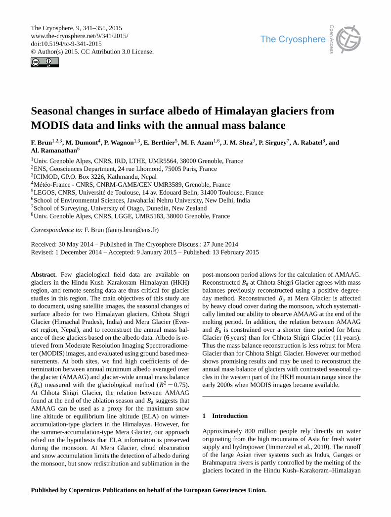
Figure 2. Example of an albedo map retrieved by MODImLab over

Chhota Shigri Glacier on 7 September 2001 05:50:00 (UTC). The

bold line delimits the pixels used to average the albedo (n= 89, cor-

responding to 4.875 km2). The northern lower part of the glacier is

covered with debris and the tributaries exhibit surfaces that include

many rock outcrops. The blue dot shows the location of the AWS.

vice, and frost deposition on the sensor can increase the un-

certainty. At Mera Glacier the AWS collected data from 9

November 2009 to 10 November 2010 and from 27 Novem-

ber 2012 to 16 November 2013. At Chhota Shigri Glacier the

AWS collected data from 13 August 2012 to 2 February 2013

and from 8 July 2013 to 3 October 2013 (Fig. 4).

Snow and ice albedo are highly sensitive to cloud cover,

which affects the ratio of direct and diffuse radiation (e.g.,

Warren, 1982; Gardner and Sharp, 2010). Therefore, we fil-

tered the data to retain only those collected in clear-sky

conditions to be able to compare them to satellite-retrieved

albedo. To do so, we calculated the local clear-sky broadband

atmospheric transmissivity χ as the ratio between the value

defining the upper envelope of measured SWin at ground

level and that defining the upper envelope of SWin at the

top of the atmosphere (TOA) (Garnier and Ohmura, 1968).

We found clear-sky χ equal to 0.99 and 0.85 on Mera and

Chhota Shigri glaciers, respectively. Clear-sky days were se-

lected as the days for which χ was in the range 0.99± 4 %

for Mera Glacier and 0.85± 10 % for Chhota Shigri Glacier

at local solar noon. The lower estimated atmospheric trans-

missivity at Chhota Shigri Glacier is likely due to its lower

elevation, its sky-view factor, and the vicinity of important

aerosol sources. The very high clear-sky χ estimated above

Mera Glacier is not realistic. It is probably due to reflec-

tions on surrounding snowy slopes and/or tilting of the sen-

sor which artificially increase the incoming shortwave radi-

ation measured by the AWS. Snow and ice albedo also de-

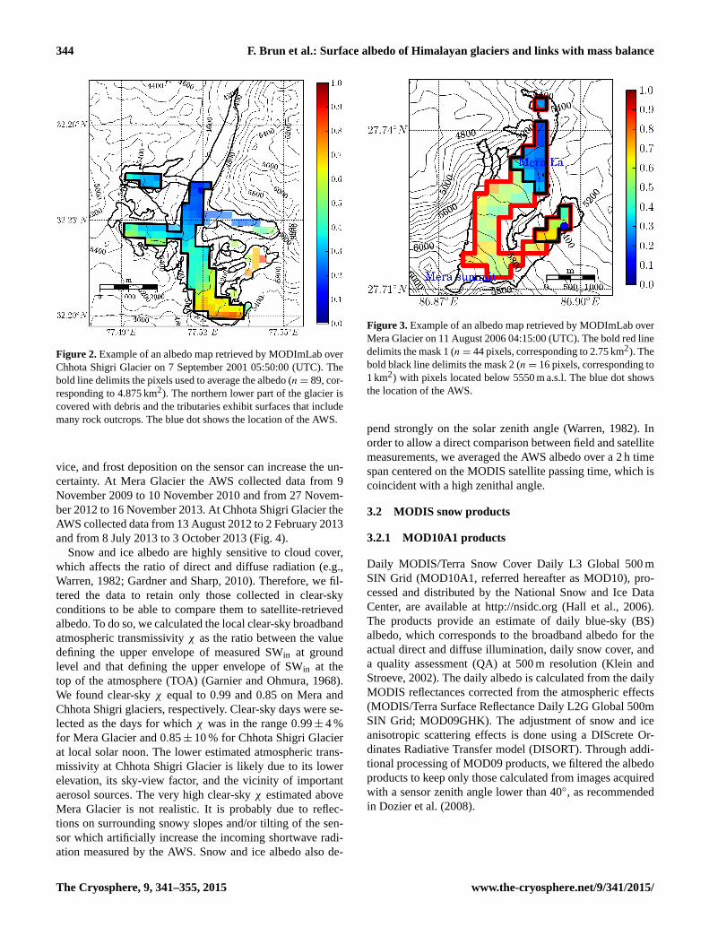
Figure 3. Example of an albedo map retrieved by MODImLab over

Mera Glacier on 11 August 2006 04:15:00 (UTC). The bold red line

delimits the mask 1 (n= 44 pixels, corresponding to 2.75 km2). The

bold black line delimits the mask 2 (n= 16 pixels, corresponding to

1 km2) with pixels located below 5550 m a.s.l. The blue dot shows

the location of the AWS.

pend strongly on the solar zenith angle (Warren, 1982). In

order to allow a direct comparison between field and satellite

measurements, we averaged the AWS albedo over a 2 h time

span centered on the MODIS satellite passing time, which is

coincident with a high zenithal angle.

3.2 MODIS snow products

3.2.1 MOD10A1 products

Daily MODIS/Terra Snow Cover Daily L3 Global 500 m

SIN Grid (MOD10A1, referred hereafter as MOD10), pro-

cessed and distributed by the National Snow and Ice Data

Center, are available at http://nsidc.org (Hall et al., 2006).

The products provide an estimate of daily blue-sky (BS)

albedo, which corresponds to the broadband albedo for the

actual direct and diffuse illumination, daily snow cover, and

a quality assessment (QA) at 500 m resolution (Klein and

Stroeve, 2002). The daily albedo is calculated from the daily

MODIS reflectances corrected from the atmospheric effects

(MODIS/Terra Surface Reflectance Daily L2G Global 500m

SIN Grid; MOD09GHK). The adjustment of snow and ice

anisotropic scattering effects is done using a DIScrete Or-

dinates Radiative Transfer model (DISORT). Through addi-

tional processing of MOD09 products, we filtered the albedo

products to keep only those calculated from images acquired

with a sensor zenith angle lower than 40◦, as recommended

in Dozier et al. (2008).

The Cryosphere, 9, 341–355, 2015 www.the-cryosphere.net/9/341/2015/

F. Brun et al.: Surface albedo of Himalayan glaciers and links with mass balance 345

Dec 09 Feb 10 Apr 10 Jun 10 Aug 10 Oct 100

200

400

600

800

1000

1200

1400

Radia

tive f

lux (

W.m

−2)

Mera

Dec 12 Feb 13 Apr 13

SWin TOA

SWin

albedo0.10.20.30.40.50.60.70.80.91.0

Alb

edo

Sep 12 Oct 12 Nov 12 Dec 12 Jan 13 Feb 130

200

400

600

800

1000

1200

1400

Radia

tive f

lux (

W.m

−2)

Chhota Shigri

Aug 13 Oct 130.10.20.30.40.50.60.70.80.9

Alb

edo

Figure 4. Measured (red) and modeled top of the atmosphere (green) incoming shortwave radiation and albedo (blue) for Chhota Shigri (top)

and Mera (bottom) glaciers. The values reported are the daily maxima of the radiative flux. The daily albedo is calculated as the average of

the albedo on a 2 h time span centered on the satellite passing time. Note the difference in x axis scale. The vertical grey lines show the days

detected as cloudy, using a threshold on incoming irradiance (see text for details).

3.2.2 MCD43 products

MODIS MCD43A3 products provide white-sky spectral

albedo (WS albedo, which corresponds to the albedo of the

surface illuminated only by diffuse irradiance), black-sky

spectral albedo (which corresponds to the albedo of the sur-

face illuminated only by direct irradiance), and broadband

albedo (called WS shortwave albedo), for the seven visi-

ble and near infrared bands of MODIS at local solar noon.

MCD43A3 products are produced at 500 m resolution ev-

ery 8 days using 16 days of MODIS Terra and Aqua acqui-

sitions. The separate products MCD43A2 are used to pro-

vide quality assessment for the MCD43A3 products. These

data are available through the online data pool at the NASA

Land Processes Distributed Active Archive Center (https:

//lpdaac.usgs.gov/).

3.2.3 MODImLab products

MODImLab is an algorithm developed to provide snow and

ice albedo with a 250 m resolution (Sirguey et al., 2009; Du-

mont et al., 2012). It retrieves albedo in mountainous regions

from MODIS TOA calibrated radiances corrected with to-

pographic and atmospheric data (see Table 1 for a complete

list of inputs and their availability). MODImLab supports

both BS albedo and WS albedo, as well as a cloud mask de-

rived from MODIS reflective and emissive bands. We filtered

the albedo products to keep only those calculated from im-

ages acquired with a sensor zenith angle lower than 40◦. For

a complete description of the albedo retrieval method, the

reader is referred to Sirguey et al. (2009), Sirguey (2009),

Dumont et al. (2011), and Dumont et al. (2012).

3.3 Glacier masks

In order to compute glacier albedo from georeferenced satel-

lite imagery provided at 250 and 500 m resolutions, we cre-

ated raster masks of the glaciers with the same resolutions

following Dumont et al. (2012). Glacier masks of 250 m reso-

lution were derived from glacier boundaries used in Wagnon

et al. (2007) and Wagnon et al. (2013), and the 500 m raster

masks derive from the 250 m masks. These masks were man-

ually defined using SPOT5 (2.5 m resolution) and Pléiades

(1 m resolution) orthoimages acquired on 21 September 2005

and 25 November 2012, respectively. They slightly differ

from the glacier outlines of the Randolph Glacier Inventory

(Pfeffer et al., 2014) but are believed to be more accurate be-

cause they have been determined based on visual inspection

of high resolution images and field expertise.

For the raster glacier mask at Chhota Shigri Glacier

(Fig. 2), we removed all pixels corresponding to debris-

covered zones (all pixels below 4500 ma.s.l. correspond-

ing to the main tongue), to rocky areas (southeastern trib-

utaries), to narrow valleys (eastern tributary) and to steep

slopes with seracs (northwestern tributary), which might af-

fect the satellite-derived albedo. The resulting mask contains

89 pixels. As this mask is large compared to other studies

(Dumont et al., 2012 used a 29 pixel mask), a mean albedo

can be assessed for the glacier even when it is partially cloud

covered (applied coverage threshold is 20 %). In contrast, for

Mera Glacier we defined two separate masks to conduct a

parallel analysis. Mask 1 (red line in Fig. 3) includes the

whole glacier (44 pixels). Conversely, we retained only the

16 pixels corresponding to elevations lower than the ELA0

(5550 ma.s.l.) for mask 2 (black line in Fig. 3). We pro-

ceeded in this way because Mera Glacier is almost always

covered by clouds during the second half of the ablation sea-

www.the-cryosphere.net/9/341/2015/ The Cryosphere, 9, 341–355, 2015

346 F. Brun et al.: Surface albedo of Himalayan glaciers and links with mass balance

Table 1. MODImLab inputs.

Data name Description Availability

MOD02QKM TOA radiances for bands 1 and 2; 250 m resolution ladsweb.nascom.nasa.gov

MOD02HKM TOA radiances for bands 3 to 7; 500 m resolution ladsweb.nascom.nasa.gov

MOD021KM TOA radiances for bands 8 to 36; 1 km resolution ladsweb.nascom.nasa.gov

MOD03 Geolocation; 1 km resolution ladsweb.nascom.nasa.gov

GDEM ASTER DEM at ∼ 30 m resolution resampled at

125 m resolution

asterweb.jpl.nasa.gov

Aeronet AOD AOD measured at Ev-K2-CNR-Pyramid; data

available from Apr 2006 to May 2011

aeronet.gsfc.nasa.gov

OMI Total ozone column; data available from Jul 2004;

1◦ resolution

ozoneaq.gsfc.nasa.gov

son (end of July to September). Further, for such a summer-

accumulation type glacier, the satellite images obtained im-

mediately after the monsoon already exhibit snow accumula-

tion at higher elevations, hiding the glacier surface represen-

tative of the end of ablation season. Moreover, calculating the

albedo on a small part of the glacier (for mask 2) increases

the availability of good quality images, especially when the

higher part of the glacier is covered by clouds, while the

lower part remains cloud-free, which is often observed in

spring.

4 Results

4.1 Evaluation of the albedo retrieval

4.1.1 Comparison with field measurements

We compared the broadband albedo measured under clear

sky conditions at the AWSs with the BS albedo retrieved

by MODImLab and MOD10 algorithm on the correspond-

ing pixel for both glaciers (Fig. 5). While ground-based and

satellite-retrieved measurements of albedo are not directly

comparable, as their spatial and temporal resolutions dif-

fer, they will be coherent in time. Indeed, the albedo mea-

sured from the AWS comes from a 80 m2 surface, whereas

the albedo derived from satellite has been calculated over a

62 500 or 250 000 m2 surface. Additionally, the AWS albedo

is averaged over a 2 h time span centered on the satellite

passing time. As the MCD43 products provide an albedo av-

eraged over 16 days we did not compare it against instan-

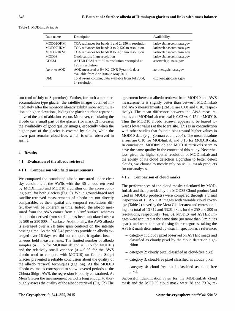
taneous field measurements. The limited number of albedo

samples (n= 15 for MODImLab and n= 16 for MOD10)

and the relatively small variance (σ = 0.05 for the AWS

albedo used to compare with MOD10) on Chhota Shigri

Glacier prevented a reliable conclusion about the quality of

the albedo retrieval techniques (Fig. 5a). As the MOD10

albedo estimates correspond to snow-covered periods at the

Chhota Shigri AWS, the regression is poorly constrained. At

Mera Glacier the measurement period is long enough to thor-

oughly assess the quality of the albedo retrieval (Fig. 5b).The

agreement between albedo retrieval from MOD10 and AWS

measurements is slightly better than between MODImLab

and AWS measurements (RMSE are 0.08 and 0.10, respec-

tively). The mean difference between the AWS measure-

ments and MODImLab retrieval is 0.03 vs. 0.15 for MOD10.

Thus the MOD10 albedo retrieval appears to be biased to-

wards lower values at the Mera site. This is in contradiction

with other studies that found a bias toward higher values in

MOD10 data (e.g., Sorman et al., 2007). The mean absolute

errors are 0.10 for MODImLab and 0.16 for MOD10 data.

In conclusion, MODImLab and MOD10 retrievals seem to

have the same quality in the context of this study. Neverthe-

less, given the higher spatial resolution of MODImLab and

the ability of its cloud detection algorithm to better detect

clouds, we choose to mostly rely on MODImLab products

for our analyses.

4.1.2 Comparison of cloud masks

The performances of the cloud masks calculated by MOD-

ImLab and that provided by the MOD35 Cloud product (and

used in MOD10 products) were compared through a visual

inspection of 13 ASTER images with variable cloud cover-

age (Table 2) covering the Mera Glacier area and correspond-

ing to a total of 13 312 and 3328 pixels for the 250 and 500 m

resolutions, respectively (Fig. 6). MODIS and ASTER im-

ages were acquired at the same time (no more than 5 minutes

apart), and were compared using four categories, taking the

ASTER mask determined by visual inspection as a reference:

– category 1: cloudy pixel observed on ASTER image and

classified as cloudy pixel by the cloud detection algo-

rithm

– category 2: cloudy pixel classified as cloud-free pixel

– category 3: cloud-free pixel classified as cloudy pixel

– category 4: cloud-free pixel classified as cloud-free

pixel.

Successful identification rates for the MODImLab cloud

mask and the MOD35 cloud mask were 78 and 73 %, re-

The Cryosphere, 9, 341–355, 2015 www.the-cryosphere.net/9/341/2015/

F. Brun et al.: Surface albedo of Himalayan glaciers and links with mass balance 347

0.0 0.2 0.4 0.6 0.8 1.0AWS albedo

(a)

0.0

0.2

0.4

0.6

0.8

1.0

MO

DIS

albe

do

MODimLabR2 = 0.87, n = 15

MOD10A1R2 = 0.46, n = 16

1:1 line

0.0 0.2 0.4 0.6 0.8 1.0AWS albedo

(b)

0.0

0.2

0.4

0.6

0.8

1.0

MO

DIS

albe

do

MODimLabR2 = 0.55, n = 68

MOD10A1R2 = 0.57, n = 80

0.0 0.5 1.0

Figure 5. Measured albedo vs. MODIS-retrieved albedo for Chhota Shigri Glacier (a) and Mera Glacier (b). For Mera Glacier RMSE are

0.10 and 0.08 for the MODImLab and the MOD10, respectively. Please note that the number of MOD10 and MODImLab images is different

because the two data set are filtered with different cloud detection algorithms. The inset represents the distribution of the measured albedo

(grey= satellite, black=AWS).

[1] [2] [3] [4]0.0

0.1

0.2

0.3

0.4

0.5

0.6

Fre

quen

cy

MODimLabMOD10

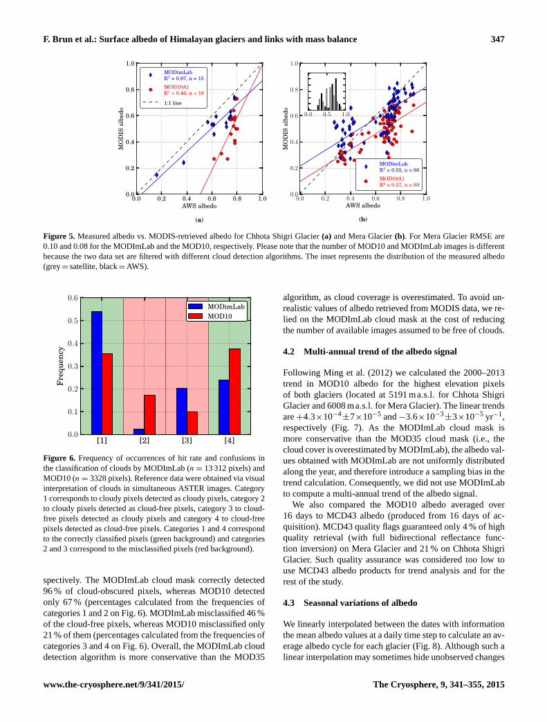
Figure 6. Frequency of occurrences of hit rate and confusions in

the classification of clouds by MODImLab (n= 13 312 pixels) and

MOD10 (n= 3328 pixels). Reference data were obtained via visual

interpretation of clouds in simultaneous ASTER images. Category

1 corresponds to cloudy pixels detected as cloudy pixels, category 2

to cloudy pixels detected as cloud-free pixels, category 3 to cloud-

free pixels detected as cloudy pixels and category 4 to cloud-free

pixels detected as cloud-free pixels. Categories 1 and 4 correspond

to the correctly classified pixels (green background) and categories

2 and 3 correspond to the misclassified pixels (red background).

spectively. The MODImLab cloud mask correctly detected

96 % of cloud-obscured pixels, whereas MOD10 detected

only 67 % (percentages calculated from the frequencies of

categories 1 and 2 on Fig. 6). MODImLab misclassified 46 %

of the cloud-free pixels, whereas MOD10 misclassified only

21 % of them (percentages calculated from the frequencies of

categories 3 and 4 on Fig. 6). Overall, the MODImLab cloud

detection algorithm is more conservative than the MOD35

algorithm, as cloud coverage is overestimated. To avoid un-

realistic values of albedo retrieved from MODIS data, we re-

lied on the MODImLab cloud mask at the cost of reducing

the number of available images assumed to be free of clouds.

4.2 Multi-annual trend of the albedo signal

Following Ming et al. (2012) we calculated the 2000–2013

trend in MOD10 albedo for the highest elevation pixels

of both glaciers (located at 5191 ma.s.l. for Chhota Shigri

Glacier and 6008 ma.s.l. for Mera Glacier). The linear trends

are+4.3×10−4±7×10−5 and−3.6×10−3

±3×10−5 yr−1,

respectively (Fig. 7). As the MODImLab cloud mask is

more conservative than the MOD35 cloud mask (i.e., the

cloud cover is overestimated by MODImLab), the albedo val-

ues obtained with MODImLab are not uniformly distributed

along the year, and therefore introduce a sampling bias in the

trend calculation. Consequently, we did not use MODImLab

to compute a multi-annual trend of the albedo signal.

We also compared the MOD10 albedo averaged over

16 days to MCD43 albedo (produced from 16 days of ac-

quisition). MCD43 quality flags guaranteed only 4 % of high

quality retrieval (with full bidirectional reflectance func-

tion inversion) on Mera Glacier and 21 % on Chhota Shigri

Glacier. Such quality assurance was considered too low to

use MCD43 albedo products for trend analysis and for the

rest of the study.

4.3 Seasonal variations of albedo

We linearly interpolated between the dates with information

the mean albedo values at a daily time step to calculate an av-

erage albedo cycle for each glacier (Fig. 8). Although such a

linear interpolation may sometimes hide unobserved changes

www.the-cryosphere.net/9/341/2015/ The Cryosphere, 9, 341–355, 2015

348 F. Brun et al.: Surface albedo of Himalayan glaciers and links with mass balance

2001 2002 2003 2004 2005 2006 2007 2008 2009 2010 2011 2012 2013

0.10.20.30.40.50.60.70.80.91.0

Alb

edo

Chhota Shigri

2001 2002 2003 2004 2005 2006 2007 2008 2009 2010 2011 2012 20130.10.20.30.40.50.60.70.80.91.0

Alb

edo

Mera

MOD1016 day average13 year trend95% confidence intervalMCD43A3

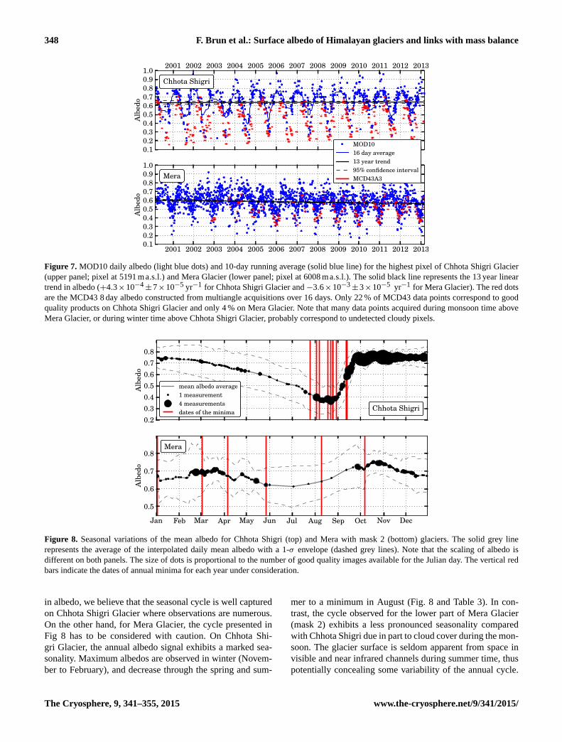
Figure 7. MOD10 daily albedo (light blue dots) and 10-day running average (solid blue line) for the highest pixel of Chhota Shigri Glacier

(upper panel; pixel at 5191 ma.s.l.) and Mera Glacier (lower panel; pixel at 6008 ma.s.l.). The solid black line represents the 13 year linear

trend in albedo (+4.3×10−4±7×10−5 yr−1 for Chhota Shigri Glacier and −3.6×10−3

±3×10−5 yr−1 for Mera Glacier). The red dots

are the MCD43 8 day albedo constructed from multiangle acquisitions over 16 days. Only 22 % of MCD43 data points correspond to good

quality products on Chhota Shigri Glacier and only 4 % on Mera Glacier. Note that many data points acquired during monsoon time above

Mera Glacier, or during winter time above Chhota Shigri Glacier, probably correspond to undetected cloudy pixels.

0.20.30.40.50.60.70.8

Alb

edo

Chhota Shigri

mean albedo average1 measurement4 measurementsdates of the minima

Jan Feb Mar Apr May Jun Jul Aug Sep Oct Nov Dec

0.5

0.6

0.7

0.8

Alb

edo

Mera

Figure 8. Seasonal variations of the mean albedo for Chhota Shigri (top) and Mera with mask 2 (bottom) glaciers. The solid grey line

represents the average of the interpolated daily mean albedo with a 1-σ envelope (dashed grey lines). Note that the scaling of albedo is

different on both panels. The size of dots is proportional to the number of good quality images available for the Julian day. The vertical red

bars indicate the dates of annual minima for each year under consideration.

in albedo, we believe that the seasonal cycle is well captured

on Chhota Shigri Glacier where observations are numerous.

On the other hand, for Mera Glacier, the cycle presented in

Fig 8 has to be considered with caution. On Chhota Shi-

gri Glacier, the annual albedo signal exhibits a marked sea-

sonality. Maximum albedos are observed in winter (Novem-

ber to February), and decrease through the spring and sum-

mer to a minimum in August (Fig. 8 and Table 3). In con-

trast, the cycle observed for the lower part of Mera Glacier

(mask 2) exhibits a less pronounced seasonality compared

with Chhota Shigri due in part to cloud cover during the mon-

soon. The glacier surface is seldom apparent from space in

visible and near infrared channels during summer time, thus

potentially concealing some variability of the annual cycle.

The Cryosphere, 9, 341–355, 2015 www.the-cryosphere.net/9/341/2015/

F. Brun et al.: Surface albedo of Himalayan glaciers and links with mass balance 349

Table 2. Acquisition dates of the ASTER images used to assess the

quality of the different cloud masks.

Date of Percentage

the image of clouds

23 May 2000 81 %

14 Oct 2000 30 %

23 Mar 2001 49 %

24 Apr 2001 2 %

26 May 2001 100 %

11 Apr 2002 11 %

9 Oct 2004 22 %

22 Jan 2008 98 %

17 Mar 2008 46 %

26 Mar 2008 22 %

2 Apr 2008 66 %

7 Jun 2011 96 %

4 Oct 2011 77 %

Consequently, when the glacier can be observed again after

the monsoon, it is mostly snow covered, even in the ablation

area, and has a relatively high albedo (' 0.7).

For Mera Glacier, the 16-day average curve of MOD10

products shown in Fig. 7 exhibits a stronger seasonality.

Given that the detection rate of clouds by MOD35 cloud

mask is relatively low (67 %, Fig. 6) and that the cloud cov-

erage during monsoon season is heavy, the albedo minima

visible on Fig. 7 are potentially artifacts due to pixel misclas-

sification. Consequently, the albedo annual cycle observed on

Fig. 7 cannot be fully considered as a true cycle.

4.4 Albedo and annual glacier-wide mass balance

The mean albedo of a glacier has been recognized as be-

ing a potentially good proxy for the transient snow line alti-

tude because of the contrast in albedo between snow and ice

(Dumont et al., 2012). Among selected Alpine glaciers regu-

larly surveyed, the altitude of the transient snow line reaches

a maximum at the end of the ablation season which corre-

sponds to the ELA (Rabatel et al., 2005). In turn, the mean

albedo of the glacier surface reaches a minimum and can ef-

fectively be used as a proxy to estimate the ELA.

We processed daily MODIS data from May 2000 to De-

cember 2013 for the two glaciers. Daily maps of WS albedo

were calculated for the two glaciers and averaged over cloud-

free glacierized pixels for images with a cloud coverage over

the glacier lower than 20 % for Chhota Shigri Glacier and

0 % for Mera Glacier (Figs. 2 and 3). WS albedo does not

depend on solar zenith angle, and is thus a more relevant

variable than BS albedo to compare albedo maps generated

at different dates, and therefore with different solar illumina-

tion. Variations in WS albedo can be interpreted more readily

as a variation in characteristics of the surface.

Table 3. Values of the observed minima of the mean albedo and

dates at which they are observed. At Mera Glacier, minimum albedo

dates can occur between 1 August and 30 June of the following year.

The data used for the calibration are in bold.

Year Chhota Shigri Mera (mask 2)

99–00 4 Sep 2000 0.263 10 Feb 2001 0.553

00–01 27 Aug 2001 0.217 18 Apr 2002 0.660

01–02 9 Aug 2002 0.243 27 Mar 2003 0.593

02–03 25 Jul 2003 0.219 29 Mar 2004 0.498

03–04 13 Sep 2004 0.246 23 May 2005 0.509

04–05 22 Aug 2005 0.318 30 Jan 2006 0.395

05–06 18 Aug 2006 0.236 3 Jul 2007 0.442

06–07 30 Aug 2007 0.287 9 Apr 2008 0.730

07–08 7 Aug 2008 0.237 2 Mar 2009 0.514

08–09 25 Aug 2009 0.356 6 Apr 2010 0.501

09–10 3 Aug 2010 0.446 27 May 2011 0.469

10–11 12 Sep 2011 0.468 10 Aug 2011 0.545

11–12 12 Sep 2012 0.286 1 Jan 2013 0.474

12–13 25 Aug 2013 0.270 7 Oct 2013 0.485

Following Dumont et al. (2012) we extracted the minimum

value of the albedo signal for the period corresponding to the

end of the ablation season of Chhota Shigri Glacier. From

field observations and precipitation regime, the snow line

was expected to be at its highest elevation between late July

and late September. Consequently, we processed images sys-

tematically from July to December and only partially for the

rest of the year to reduce the amount of L1B data to be down-

loaded and processed. Minimum albedo values range from

0.22 to 0.46, and the AMAAG correlates well with the field-

based measurements of Ba (Fig. 9a). This is supported by

a determination coefficient (R2) equal to 0.75 (n= 11 years;

significant at 95 % confidence with a Student’s t test). The

agreement is better for negative mass balance years. All the

dates of the observed minimum albedo are between 25 July

and 13 September (Table 3). It is also noteworthy that the

AMAAG values are scattered when Ba is 0 or slightly posi-

tive for Chhota Shigri Glacier.

On Mera Glacier the snow line was expected to be the

highest at the end of the monsoon season (between August

and September) during which most of the ablation and ac-

cumulation occur (Wagnon et al., 2013). Unfortunately, the

minimum albedo value during these months could hardly be

observed from space because of the persistent cloud cover-

age during this period. On the first images captured after the

monsoon, the glacier is usually covered by snow that likely

conceals the ELA information. Nevertheless, Wagnon et al.

(2013) observed that between October and April, the snow

deposited above Mera La (5400 ma.s.l., Fig. 3) is systemati-

cally re-mobilized or sublimated by strong winds. As a con-

sequence, the surface representative of the glacier at the end

of the previous monsoon season, unfortunately not visible

from space at this period, is likely to be exposed again in the

www.the-cryosphere.net/9/341/2015/ The Cryosphere, 9, 341–355, 2015

350 F. Brun et al.: Surface albedo of Himalayan glaciers and links with mass balance

−2.0 −1.5 −1.0 −0.5 0.0 0.5 1.0Annual mass balance (m w.e.)

(a)

0.20

0.25

0.30

0.35

0.40

0.45

0.50

Min

imum

mea

nal

bedo

duri

ngth

eab

lati

onse

ason

02-03

03-04

04-05

05-06

06-07

07-08

08-09

11-1212-13

10-1109-10

Chhota ShigriR2 = 0.75slope = 0.11±0.01 m w.e.−1

intercept = 0.37Sdt error = 0.021n = 11

−1.0 −0.8 −0.6 −0.4 −0.2 0.0 0.2 0.4 0.6 0.8Annual mass balance (m w.e.)

(c)

0.44

0.46

0.48

0.50

0.52

0.54

0.56

Min

imum

mea

nal

bedo

duri

ngth

efo

llow

ing

year

07-08

08-09

09-10

10-11

11-12

12-13

Mera - Mask 2R2 = 0.75slope = 0.05±0.02 m w.e.−1

intercept = 0.50Sdt error = 0.015n = 6

−1.0 −0.8 −0.6 −0.4 −0.2 0.0 0.2 0.4Annual mass balance (m w.e.)

(b)

0.50

0.55

0.60

0.65

0.70

0.75

0.80

Min

imum

mea

nal

bedo

duri

ngth

efo

llow

ing

year

07-0808-09

09-10

10-11

11-12

12-13

Mera - Mask 1R2 = 0.13slope = 0.04±0.01 m w.e.−1

intercept = 0.63Sdt error = 0.053n = 6

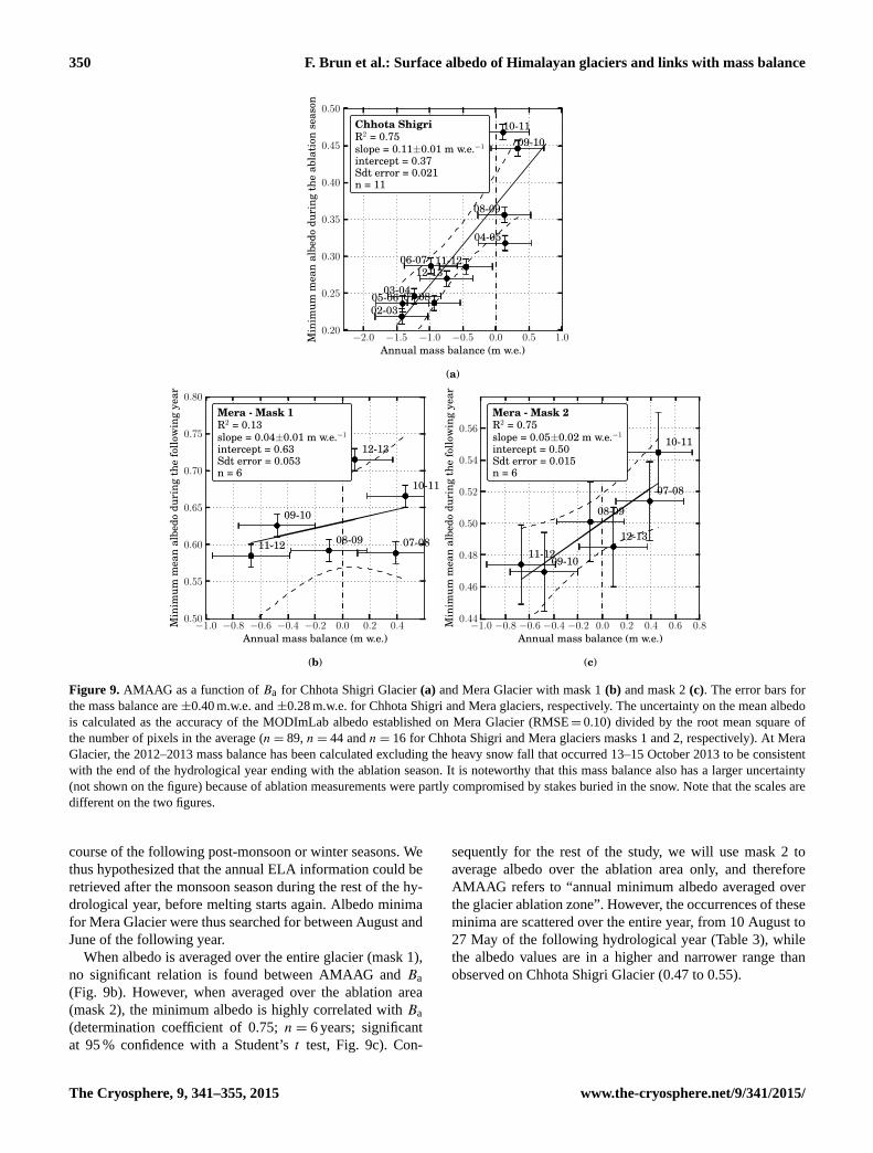
Figure 9. AMAAG as a function of Ba for Chhota Shigri Glacier (a) and Mera Glacier with mask 1 (b) and mask 2 (c). The error bars for

the mass balance are ±0.40 m.w.e. and ±0.28 m.w.e. for Chhota Shigri and Mera glaciers, respectively. The uncertainty on the mean albedo

is calculated as the accuracy of the MODImLab albedo established on Mera Glacier (RMSE= 0.10) divided by the root mean square of

the number of pixels in the average (n= 89, n= 44 and n= 16 for Chhota Shigri and Mera glaciers masks 1 and 2, respectively). At Mera

Glacier, the 2012–2013 mass balance has been calculated excluding the heavy snow fall that occurred 13–15 October 2013 to be consistent

with the end of the hydrological year ending with the ablation season. It is noteworthy that this mass balance also has a larger uncertainty

(not shown on the figure) because of ablation measurements were partly compromised by stakes buried in the snow. Note that the scales are

different on the two figures.

course of the following post-monsoon or winter seasons. We

thus hypothesized that the annual ELA information could be

retrieved after the monsoon season during the rest of the hy-

drological year, before melting starts again. Albedo minima

for Mera Glacier were thus searched for between August and

June of the following year.

When albedo is averaged over the entire glacier (mask 1),

no significant relation is found between AMAAG and Ba

(Fig. 9b). However, when averaged over the ablation area

(mask 2), the minimum albedo is highly correlated with Ba

(determination coefficient of 0.75; n= 6 years; significant

at 95 % confidence with a Student’s t test, Fig. 9c). Con-

sequently for the rest of the study, we will use mask 2 to

average albedo over the ablation area only, and therefore

AMAAG refers to “annual minimum albedo averaged over

the glacier ablation zone”. However, the occurrences of these

minima are scattered over the entire year, from 10 August to

27 May of the following hydrological year (Table 3), while

the albedo values are in a higher and narrower range than

observed on Chhota Shigri Glacier (0.47 to 0.55).

The Cryosphere, 9, 341–355, 2015 www.the-cryosphere.net/9/341/2015/

F. Brun et al.: Surface albedo of Himalayan glaciers and links with mass balance 351

−2.0

−1.5

−1.0

−0.5

0.0

0.5

1.0

Mas

sba

lanc

e(m

w.e

.)

Chhota Shigri

Azam et al., 2014

2000 2002 2004 2006 2008 2010 2012 2014−1.5−1.0−0.5

0.00.51.01.52.02.53.0

Mas

sba

lanc

e(m

w.e

.)

Mera reconstructed MBfield MBgeodetic MBaverage of reconstructed MB

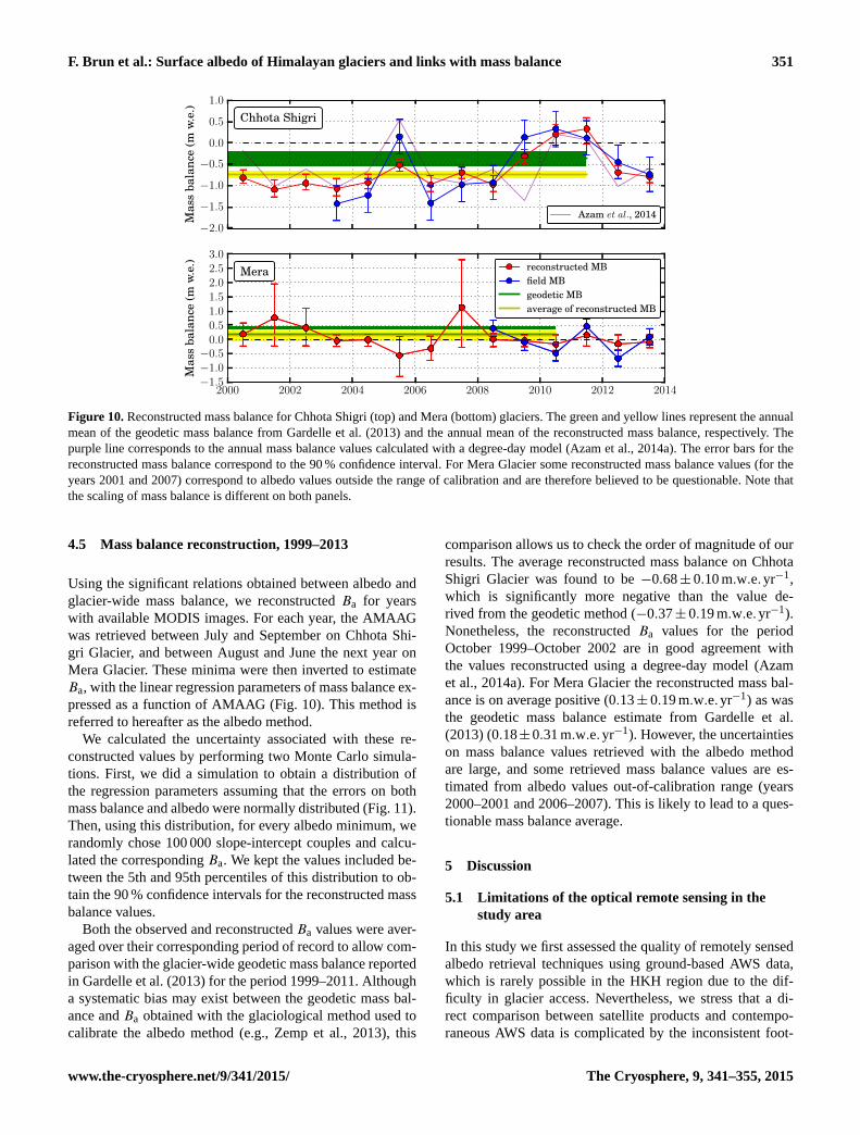
Figure 10. Reconstructed mass balance for Chhota Shigri (top) and Mera (bottom) glaciers. The green and yellow lines represent the annual

mean of the geodetic mass balance from Gardelle et al. (2013) and the annual mean of the reconstructed mass balance, respectively. The

purple line corresponds to the annual mass balance values calculated with a degree-day model (Azam et al., 2014a). The error bars for the

reconstructed mass balance correspond to the 90 % confidence interval. For Mera Glacier some reconstructed mass balance values (for the

years 2001 and 2007) correspond to albedo values outside the range of calibration and are therefore believed to be questionable. Note that

the scaling of mass balance is different on both panels.

4.5 Mass balance reconstruction, 1999–2013

Using the significant relations obtained between albedo and

glacier-wide mass balance, we reconstructed Ba for years

with available MODIS images. For each year, the AMAAG

was retrieved between July and September on Chhota Shi-

gri Glacier, and between August and June the next year on

Mera Glacier. These minima were then inverted to estimate

Ba, with the linear regression parameters of mass balance ex-

pressed as a function of AMAAG (Fig. 10). This method is

referred to hereafter as the albedo method.

We calculated the uncertainty associated with these re-

constructed values by performing two Monte Carlo simula-

tions. First, we did a simulation to obtain a distribution of

the regression parameters assuming that the errors on both

mass balance and albedo were normally distributed (Fig. 11).

Then, using this distribution, for every albedo minimum, we

randomly chose 100 000 slope-intercept couples and calcu-

lated the corresponding Ba. We kept the values included be-

tween the 5th and 95th percentiles of this distribution to ob-

tain the 90 % confidence intervals for the reconstructed mass

balance values.

Both the observed and reconstructed Ba values were aver-

aged over their corresponding period of record to allow com-

parison with the glacier-wide geodetic mass balance reported

in Gardelle et al. (2013) for the period 1999–2011. Although

a systematic bias may exist between the geodetic mass bal-

ance and Ba obtained with the glaciological method used to

calibrate the albedo method (e.g., Zemp et al., 2013), this

comparison allows us to check the order of magnitude of our

results. The average reconstructed mass balance on Chhota

Shigri Glacier was found to be −0.68± 0.10 m.w.e.yr−1,

which is significantly more negative than the value de-

rived from the geodetic method (−0.37± 0.19 m.w.e.yr−1).

Nonetheless, the reconstructed Ba values for the period

October 1999–October 2002 are in good agreement with

the values reconstructed using a degree-day model (Azam

et al., 2014a). For Mera Glacier the reconstructed mass bal-

ance is on average positive (0.13± 0.19 m.w.e.yr−1) as was

the geodetic mass balance estimate from Gardelle et al.

(2013) (0.18±0.31 m.w.e.yr−1). However, the uncertainties

on mass balance values retrieved with the albedo method

are large, and some retrieved mass balance values are es-

timated from albedo values out-of-calibration range (years

2000–2001 and 2006–2007). This is likely to lead to a ques-

tionable mass balance average.

5 Discussion

5.1 Limitations of the optical remote sensing in the

study area

In this study we first assessed the quality of remotely sensed

albedo retrieval techniques using ground-based AWS data,

which is rarely possible in the HKH region due to the dif-

ficulty in glacier access. Nevertheless, we stress that a di-

rect comparison between satellite products and contempo-

raneous AWS data is complicated by the inconsistent foot-

www.the-cryosphere.net/9/341/2015/ The Cryosphere, 9, 341–355, 2015

352 F. Brun et al.: Surface albedo of Himalayan glaciers and links with mass balance

Figure 11. Regression parameters obtained from the Monte Carlo

simulation (N = 10 000). Every data point represents a slope-

intercept couple obtained as the best fit of Ba as a function of

AMAAG.

print of both measurement techniques. The satellite re-

trieval is a quantity integrated over 62 500 m2 for MOD-

ImLab (250 m× 250 m, approximately one pixel area) and

250 000 m2 for MOD10 product (500 m× 500 m, approxi-

mately one pixel area), while the AWS sensor’s footprint is

approximately 80 m2 (99% of the radiation reaching the sen-

sor come from a 10×h diameter disc, where h= 1 m is the

sensor height above the surface). Consequently, the albedo

retrieved from satellite data is more likely to involve a ra-

diometric mixture (pixel partially covered by ice and snow),

whereas the albedo retrieved by the AWS corresponds to

a more homogeneous surface, either covered by snow or ice,

as illustrated by the marked bimodal distribution of observed

albedo values shown in Fig. 5b (inset). Such inconsistency

is more likely when the AWS is set close to the expected

ELA, where more mixed pixels comprised of snow and ice

are expected. In view of this limitation, one may consider

that MODImLab albedo maps only capture the variations of

albedo at the glacier scale.

The relatively high rate of misclassification of cloudy pix-

els (33 %) in MOD10 products raises questions about the

significance of the calculated decadal trend. In addition to

the sampling problem associated with the persistent cloud

coverage during winter time on Chhota Shigri Glacier and

monsoon season on Mera Glacier, the observed decadal

trends might not be related to changes in the glacier sur-

face, but could also be related to changes occurring in the

atmosphere or due to a drift in MODIS sensors calibration

(e.g., Zhang and Reid, 2010). Nevertheless these trends are

consistent with those observed by Ming et al. (2012), at

glaciers PT1 and PT4, which are located relatively close to

Chhota Shigri and Mera glaciers. Albedo trends at PT1 and

PT4, respectively, are +6.4× 10−3 and −1.1× 10−3 yr−1.

Albedo trends at Chhota Shigri Glacier and Mera Glacier are

+4.3×10−4±7×10−5 and−3.6×10−3

±3×10−5 yr−1, re-

spectively. These trends are both significant for a confidence

level of 85 % with a Student’s t test. Ming et al. (2012) ob-

served only negative albedo trends except for the most west-

ern glacier of their study PT1. The positive trend we obtained

at Chhota Shigri Glacier, close to PT1, seems to confirm this

finding.

Special cloud detection algorithms are required in moun-

tainous and high altitude regions (Hall and Riggs, 2007; Sir-

guey et al., 2009). In particular, thresholds on the differ-

ent bands, band ratios, and band combinations need adjust-

ments when applied to different regions. For instance, the

relatively low water vapor content of the atmosphere above

Mera Glacier (clear sky χ of 0.99) yields frequent misclassi-

fications of cloud free pixels as high altitude clouds in MOD-

ImLab cloud detection algorithm. Our work suggests that in-

dependent tuning of cloud detection algorithms is required,

and this requires extensive comparison with other interpreted

images, a process that is both time consuming and operator

dependent.

5.2 Advantages, drawbacks, and robustness of the

albedo method applied in the Himalayas

An attractive application of the albedo method is to recon-

struct Ba for periods when surface observations are not avail-

able. The mass balance reconstruction is robust for Chhota

Shigri Glacier but appeared questionable for Mera Glacier.

We suggest three main reasons for this difference.

First, the choice of pixels included in Mera Glacier mask

is questionable. In our case selecting only the lower part of

the glacier lead to a strong improvement in the correlation

between Ba and AMAAG (Fig. 9b and c). This approach is

only suitable for glaciers where ELA0 is known. As mask

2 includes only pixels located below the ELA0 (Fig. 3), the

mean albedo cannot be related to ELA detection in the cases

when ELA is above ELA0 (i.e., negative Ba observed for

years 2008–2009, 2009–2010 and 2011–2012).

Second, persistent cloud coverage at Mera Glacier does

not allow the true AMAAG to be resolved in some years.

In order to test this hypothesis we also considered the sec-

ond lowest value of the mean albedo observed between Au-

gust and June on Mera Glacier. This revealed that the sec-

ond lowest albedo value is often observed more than two

months apart from the AMAAG and often exceeds the ac-

tual observed minimum by 0.05 to 0.3. In contrast, the second

minimum mean albedo measured on Chhota Shigri Glacier is

close to the minimum (+0.01) for most years and is generally

observed within 10 days. Moreover, the visual inspection of

the albedo time series (Fig. 8) confirms a well-defined min-

imum on Chhota Shigri Glacier, whereas the seasonal cycle

of the mean albedo on Mera Glacier is poorly resolved and

less marked.

The Cryosphere, 9, 341–355, 2015 www.the-cryosphere.net/9/341/2015/

F. Brun et al.: Surface albedo of Himalayan glaciers and links with mass balance 353

Third, the relation between mass balance and AMAAG is

poorly constrained for summer accumulation-type glaciers,

where accumulation and ablation occur simultaneously. For

Mera Glacier, the range of albedo values used for calibration

is narrower than that on Chhota Shigri Glacier (0.47 to 0.55

vs. 0.21 to 0.47). It is also noteworthy that the albedo is cal-

culated from fewer pixels on Mera Glacier than on Chhota

Shigri Glacier (16 and 89, respectively), and so the mean

albedo obtained for Mera Glacier has a higher uncertainty

(Fig. 9b). The AMAAG-Ba relation is also calibrated over

a shorter period for Mera Glacier than for Chhota Shigri

Glacier (6 years vs. 11). Therefore the regression parameters

are less constrained on Mera Glacier than on Chhota Shigri

Glacier (Fig. 11), which leads to higher uncertainty.

A future application of the albedo method could be to cal-

culate mass balance of neighboring glaciers. This would re-

quire more studies to examine regression parameter from the

relation betweenBa and AMAAG in the context of glacier to-

pography and climate. These studies should preferentially be

conducted on glaciers that exhibit a strong albedo seasonal

cycle, like Chhota Shigri Glacier. Ming et al. (2012) pre-

sented the seasonal albedo cycle of 11 Himalayan glaciers,

including 7 of them with a well-defined albedo cycle that

could be suitable candidates for such a study. Two of their

studied glaciers (Naimona’nyi and East Rongbuk glaciers)

exhibit an albedo cycle with a phase opposition compared to

the others (i.e., the albedo reaches a maximum during sum-

mer and a minimum during winter), and further research into

the application of the albedo method is required for summer-

accumulation type glaciers.

6 Conclusions

In this study we presented and assessed a method to recon-

struct the annual mass balance of Himalayan glaciers from

MODIS images. This method could be applied to other re-

cently surveyed glaciers and would allow Ba to be estimated

from the hydrological year 2000 to present. The relation be-

tween Ba and the AMAAG must be calibrated over several

years with mass balance values obtained from other meth-

ods, such as the glaciological method.

Despite the intrinsic limitations of moderate resolution im-

agery (subpixel variability, exclusion of pixels at the edge of

the glacier, presence of ice and rocks mixed pixels, applica-

bility only on large glaciers), our study has successfully ap-

plied the MODImLab albedo retrieval algorithm to two Hi-

malayan sites. MODImLab is therefore believed to be a suit-

able tool to monitor glacier surface albedo in the Himalayas.

Our albedo method for mass balance reconstruction was

successful for Chhota Shigri Glacier (a winter-accumulation-

type glacier), but questionable in the case of Mera Glacier

(a summer-accumulation type glacier). While our albedo-

derived estimates of glacier mass balance are validated with

geodetic mass balance observations, time series of ground-

based mass balance data with sufficient length are still re-

quired to construct robust regression models. Spatial extrapo-

lation of these results to climatologically similar regions and

validation with geodetic mass balance estimates would pro-

vide a better indication of the transferability of our results,

and provide important information on the inter-annual vari-

ability glacier mass balance in unmonitored regions of the

Hindu Kush Himalayas.

Acknowledgements. This work has been supported by the French

Service d’Observation GLACIOCLIM, the French National Re-

search Agency (ANR) through ANR-09-CEP-005-01-PAPRIKA,

and ANR-13-SENV-0005-04-PRESHINE , and the French National

Space Center (CNES) through TOSCA and ISIS projects, and has

been supported by a grant from Labex OSUG@2020 (Investisse-

ments d’avenir – ANR10 LABX56). LTHE, CNRM-GAME/CEN

and LGGE are part of LabEx OSUG@2020. This study was

carried out within the framework of the Ev-K2-CNR Project in

collaboration with the Nepal Academy of Science and Technology

as foreseen by the Memorandum of Understanding between Nepal

and Italy, and thanks to contributions from the Italian National

Research Council, the Italian Ministry of Education, University

and Research and the Italian Ministry of Foreign Affairs. This work

has been conducted in ICIMOD and LTHE, which are greatly ac-

knowledged for their support. JMS is supported by the Cryosphere

Monitoring Project, which is funded by the Norwegian Ministry of

Foreign Affairs through the Norwegian Embassy in Kathmandu.

The authors are grateful to Kimberly Casey and Thomas Painter for

their valuable comments which greatly improved an earlier version

of this work.

Edited by: A. Kääb

References

Azam, M. F., Wagnon, P., Ramanathan, A., Vincent, C.,

Sharma, P., Arnaud, Y., Linda, A., Pottakkal, J. G., Cheval-

lier, P., Singh, V. B., and Berthier, E.: From balance to im-

balance: a shift in the dynamic behaviour of Chhota Shi-

gri glacier, western Himalaya, India, J. Glaciol., 58, 315–324,

doi:10.3189/2012JoG11J123, 2012.

Azam, M. F., Wagnon, P., Vincent, C., Ramanathan, A., Linda, A.,

and Singh, V. B.: Reconstruction of the annual mass balance of

Chhota Shigri glacier, Western Himalaya, India, since 1969, Ann.

Glaciol., 55, 69–80, doi:10.3189/2014AoG66A104, 2014a.

Azam, M. F., Wagnon, P., Vincent, C., Ramanathan, A., Favier, V.,

Mandal, A., and Pottakkal, J. G.: Processes governing the mass

balance of Chhota Shigri Glacier (western Himalaya, India) as-

sessed by point-scale surface energy balance measurements, The

Cryosphere, 8, 2195–2217, doi:10.5194/tc-8-2195-2014, 2014b.

Berthier, E., Arnaud, Y., Kumar, R., Ahmad, S., Wagnon, P., and

Chevallier, P.: Remote sensing estimates of glacier mass balances

in the Himachal Pradesh (Western Himalaya, India), Remote

Sens. Environ., 108, 327–338, doi:10.1016/j.rse.2006.11.017,

2007.

www.the-cryosphere.net/9/341/2015/ The Cryosphere, 9, 341–355, 2015

354 F. Brun et al.: Surface albedo of Himalayan glaciers and links with mass balance

Bolch, T., Pieczonka, T., and Benn, D. I.: Multi-decadal mass loss

of glaciers in the Everest area (Nepal Himalaya) derived from

stereo imagery, The Cryosphere, 5, 349–358, doi:10.5194/tc-5-

349-2011, 2011.

Bolch, T., Kulkarni, A., Kääb, A., Huggel, C., Paul, F., Cogley, J.,

Frey, H., Kargel, J., Fujita, K., Scheel, M., Bajracharya, S., and

Stoffel, M.: The state and fate of Himalayan glaciers, Science,

336, 310–314, doi:10.1126/science.1215828, 2012.

Bookhagen, B. and Burbank, D. W.: Topography, relief, and

TRMM-derived rainfall variations along the Himalaya, Geophys.

Res. Lett., 33, L08405, doi:10.1029/2006GL026037, 2006.

Bookhagen, B. and Burbank, D. W.: Toward a complete Himalayan

hydrological budget: spatiotemporal distribution of snowmelt

and rainfall and their impact on river discharge, J. Geophys. Res.-

Earth, 115, F03019, doi:10.1029/2009JF001426, 2010.

Burbank, D. W., Bookhagen, B., Gabet, E. J., and Putkonen, J.:

Modern climate and erosion in the Himalaya, CR Geosci., 314,

610–626, doi:10.1016/j.crte.2012.10.010, 2012.

Dozier, J., Painter, T. H., Rittger, K., and Frew, J. E.: Time-

space continuity of daily maps of fractional snow cover and

albedo from MODIS, Adv. Water Resour., 31, 1515–1526,

doi:10.1016/j.advwatres.2008.08.011, 2008.

Dumont, M., Sirguey, P., Arnaud, Y., and Six, D.: Monitoring spatial

and temporal variations of surface albedo on Saint Sorlin Glacier

(French Alps) using terrestrial photography, The Cryosphere, 5,

759–771, doi:10.5194/tc-5-759-2011, 2011.

Dumont, M., Gardelle, J., Sirguey, P., Guillot, A., Six, D., Raba-

tel, A., and Arnaud, Y.: Linking glacier annual mass balance and

glacier albedo retrieved from MODIS data, The Cryosphere, 6,

1527–1539, doi:10.5194/tc-6-1527-2012, 2012.

Fyffe, C. L., Tim, D., Brock, B. W., Kirkbride, M. P., Diolaiuti, G.,

Smiraglia, C., and Diotri, F.: A distributed energy-balance melt

model of an alpine debris-covered glacier, J. Glaciol., 60, 587–

602, doi:10.3189/2014JoG13J045, 2014.

Gardelle, J., Berthier, E., Arnaud, Y., and Kääb, A.: Region-wide

glacier mass balances over the Pamir-Karakoram-Himalaya dur-

ing 1999–2011, The Cryosphere, 7, 1263–1286, doi:10.5194/tc-

7-1263-2013, 2013.

Gardner, A. S. and Sharp, M. J.: A review of snow and ice

albedo and the development of a new physically based broadband

albedo parameterization, J. Geophys. Res.-Earth, 115, F01009,

doi:10.1029/2009JF001444, 2010.

Gardner, A. S., Moholdt, G., Cogley, J. G., Wouters, B.,

Arendt, A. A., Wahr, J., Berthier, E., Hock, R., Pfeffer, W. T.,

Kaser, G., Ligtenberg, S. R. M., Bolch, T., Sharp, M. J., Ha-

gen, J. O., van den Broeke, M. R., and Paul, F.: A reconciled

estimate of glacier contributions to sea level rise: 2003 to 2009,

Science, 340, 852–857, doi:10.1126/science.1234532, 2013.

Garnier, B. and Ohmura, A.: A method of calculating the direct

shortwave radiation income of slopes, J. Appl. Meteorol., 7, 796–

800, 1968.

Hall, D. K. and Riggs, G. A.: Accuracy assessment of the

MODIS snow products, Hydrol. Process., 21, 1534–1547,

doi:10.1002/hyp.6715, 2007.

Hall, D. K., Riggs, G. A., and Salomonson, V. V.: MODIS/Terra

Snow Cover Daily L3 Global 500 m Grid V005, 2000–2013, Na-

tional Snow and Ice Data Center, Digital media, Boulder, Col-

orado, USA, 2006 (updated daily).

Hatwar, H., Yadav, B., Ramarao, Y., and Parikh, R.: Prediction of

western disturbances and associated weather over western Hi-

malayas, Curr. Sci. India, 88, 913–920, 2005.

Immerzeel, W., Pellicciotti, F., and Bierkens, M.: Rising river flows

throughout the twenty-first century in two Himalayan glacierized

watersheds, Nat. Geosci., 6, 742–745, doi:10.1038/NGEO1896,

2013.

Immerzeel, W. W., van Beek, L. P., and Bierkens, M. F.: Climate

change will affect the Asian water towers, Science, 328, 1382–

1385, doi:10.1126/science.1183188, 2010.

Jacob, T., Wahr, J., Pfeffer, W. T., and Swenson, S.: Recent con-

tributions of glaciers and ice caps to sea level rise, Nature, 482,

514–518, doi:10.1038/nature10847, 2012.

Kääb, A., Berthier, E., Nuth, C., Gardelle, J., and Ar-

naud, Y.: Contrasting patterns of early twenty-first-century

glacier mass change in the Himalayas, Nature, 488, 495–498,

doi:10.1038/nature11324, 2012.

Kaser, G., Großhauser, M., and Marzeion, B.: Contribution

potential of glaciers to water availability in different cli-

mate regimes, P. Natl. Acad. Sci. USA, 107, 20223–20227,

doi:10.1073/pnas.1008162107, 2010.

Klein, A. G. and Stroeve, J.: Development and validation of a snow

albedo algorithm for the MODIS instrument, Ann. Glaciol., 34,

45–52, 2002.

Lejeune, Y., Bertrand, J.-M., Wagnon, P., and Morin, S.: A phys-

ically based model of the year-round surface energy and mass

balance of debris-covered glaciers, J. Glaciol., 59, 327–344,

doi:10.3189/2013JoG12J149, 2013.

Maussion, F., Scherer, D., Mölg, T., Collier, E., Curio, J., and

Finkelnburg, R.: Precipitation seasonality and variability over the

Tibetan Plateau as resolved by the High Asia Reanalysis, J. Cli-

mate, 27, 1910–1927, doi:10.1175/JCLI-D-13-00282.1, 2013.

Ming, J., Du, Z., Xiao, C., Xu, X., and Zhang, D.: Darkening of the

mid-Himalaya glaciers since 2000 and the potential causes, Env-

iron. Res. Lett., 7, 014021, doi:10.1088/1748-9326/7/1/014021,

2012.

Nicholson, L. and Benn, D. I.: Calculating ice melt beneath a de-

bris layer using meteorological data, J. Glaciol., 52, 463–470,

doi:10.3189/172756506781828584, 2006.

Nuimura, T., Fujita, K., Yamaguchi, S., and Sharma, R. R.: Ele-

vation changes of glaciers revealed by multitemporal digital el-

evation models calibrated by GPS survey in the Khumbu re-

gion, Nepal Himalaya, 1992–2008, J. Glaciol., 58, 648–656,

doi:10.3189/2012JoG11J061, 2012.

Pfeffer, W. T., Arendt, A. A., Bliss, A., Bolch, T., Cogley, J. G.,

Gardner, A. S., Hagen, J.-O., Hock, R., Kaser, G., Kienholz, C.,

Miles, E. S., Moholdt, G., Mölg, N., Paul, F., Radic, V., Rastner,

P., Raup, B. H., Rich, J., and Sharp, M. J.: The Randolph Glacier

Inventory: a globally complete inventory of glaciers, J. Glaciol.,

60, 537–552, doi:10.3189/2014JoG13J176, 2014.

Rabatel, A., Dedieu, J.-P., and Vincent, C.: Using remote-sensing

data to determine equilibrium-line altitude and mass-balance

time series: validation on three French glaciers, 1994–2002, J.

Glaciol., 51, 539–546, 2005.

Rabatel, A., Letréguilly, A., Dedieu, J.-P., and Eckert, N.: Changes

in glacier equilibrium-line altitude in the western Alps from

1984 to 2010: evaluation by remote sensing and modeling of

the morpho-topographic and climate controls, The Cryosphere,

7, 1455–1471, doi:10.5194/tc-7-1455-2013, 2013.

The Cryosphere, 9, 341–355, 2015 www.the-cryosphere.net/9/341/2015/

F. Brun et al.: Surface albedo of Himalayan glaciers and links with mass balance 355

Radic, V., Bliss, A., Beedlow, A., Hock, R., Miles, E., and

Cogley, J.: Regional and global projections of twenty-first

century glacier mass changes in response to climate scenar-

ios from global climate models, Clim. Dynam., 42, 37–58,

doi:10.1007/s00382-013-1719-7, 2014.

Richardson, S. D. and Reynolds, J. M.: An overview of glacial haz-

ards in the Himalayas, Quatern. Int., 65, 31–47, 2000.

Scherler, D., Bookhagen, B., and Strecker, M. R.: Spatially variable

response of Himalayan glaciers to climate change affected by

debris cover, Nat. Geosci., 4, 156–159, doi:10.1038/ngeo1068,

2011.

Shea, J. M., Menounos, B., Moore, R. D., and Tennant, C.: An ap-

proach to derive regional snow lines and glacier mass change

from MODIS imagery, western North America, The Cryosphere,

7, 667–680, doi:10.5194/tc-7-667-2013, 2013.

Shrestha, D., Singh, P., and Nakamura, K.: Spatiotemporal vari-

ation of rainfall over the central Himalayan region revealed

by TRMM Precipitation Radar, J. Geophys. Res.-Atmos., 117,

D22106, doi:10.1029/2012JD018140, 2012.

Sirguey, P.: Simple correction of multiple reflection effects

in rugged terrain, Int. J. Remote Sens., 30, 1075–1081,

doi:10.1080/01431160802348101, 2009.

Sirguey, P., Mathieu, R., and Arnaud, Y.: Subpixel monitoring of

the seasonal snow cover with MODIS at 250m spatial resolu-

tion in the Southern Alps of New Zealand: Methodology and

accuracy assessment, Remote Sens. Environ., 113, 160–181,

doi:10.1016/j.rse.2008.09.008, 2009.

Sorman, A. Ü., Akyürek, Z., Sensoy, A., Sorman, A. A., and

Tekeli, A. E.: Commentary on comparison of MODIS snow

cover and albedo products with ground observations over the

mountainous terrain of Turkey, Hydrol. Earth Syst. Sci., 11,

1353–1360, doi:10.5194/hess-11-1353-2007, 2007.

Thibert, E., Blanc, R., Vincent, C., and Eckert, N.: Instruments

and Methods Glaciological and volumetric mass-balance mea-

surements: error analysis over 51 years for Glacier de Sarennes,

French Alps, J. Glaciol., 54, 522–532, 2008.

Vincent, C., Ramanathan, Al., Wagnon, P., Dobhal, D. P., Linda, A.,

Berthier, E., Sharma, P., Arnaud, Y., Azam, M. F., Jose, P. G., and

Gardelle, J.: Balanced conditions or slight mass gain of glaciers

in the Lahaul and Spiti region (northern India, Himalaya) during

the nineties preceded recent mass loss, The Cryosphere, 7, 569–

582, doi:10.5194/tc-7-569-2013, 2013.

Wagnon, P., Linda, A., Arnaud, Y., Kumar, R., Sharma, P., Vin-

cent, C., Pottakkal, J. G., Berthier, E., Ramanathan, A., Has-

nain, S. I., and Chevallier, P.: Four years of mass balance on

Chhota Shigri Glacier, Himachal Pradesh, India, a new bench-

mark glacier in the western Himalaya, J. Glaciol., 53, 603–611,

2007.

Wagnon, P., Vincent, C., Arnaud, Y., Berthier, E., Vuillermoz, E.,

Gruber, S., Ménégoz, M., Gilbert, A., Dumont, M., Shea, J. M.,

Stumm, D., and Pokhrel, B. K.: Seasonal and annual mass bal-

ances of Mera and Pokalde glaciers (Nepal Himalaya) since

2007, The Cryosphere, 7, 1769–1786, doi:10.5194/tc-7-1769-

2013, 2013.

Warren, S. G.: Optical properties of snow, Rev. Geophys., 20, 67–

89, doi:10.1029/RG020i001p00067, 1982.

Yao, T., Thompson, L., Yang, W., Yu, W., Gao, Y.,

Guo, X., Yang, X., Duan, K., Zhao, H.,

Xu, B,Pu, J.,Lu, A.,Xiang, Y.,Kattel, D. B., and Joswiak, D:

Different glacier status with atmospheric circulations in Tibetan

Plateau and surroundings, Nat. Clim. Change, 2, 663–667,

doi:10.1038/NCLIMATE1580, 2012.

Zemp, M., Thibert, E., Huss, M., Stumm, D., Rolstad Denby, C.,

Nuth, C., Nussbaumer, S. U., Moholdt, G., Mercer, A.,

Mayer, C., Joerg, P. C., Jansson, P., Hynek, B., Fischer, A.,

Escher-Vetter, H., Elvehøy, H., and Andreassen, L. M.: Re-

analysing glacier mass balance measurement series, The

Cryosphere, 7, 1227–1245, doi:10.5194/tc-7-1227-2013, 2013.

Zhang, J. and Reid, J. S.: A decadal regional and global trend

analysis of the aerosol optical depth using a data-assimilation

grade over-water MODIS and Level 2 MISR aerosol products,

Atmos. Chem. Phys., 10, 10949–10963, doi:10.5194/acp-10-

10949-2010, 2010.

www.the-cryosphere.net/9/341/2015/ The Cryosphere, 9, 341–355, 2015