Second Order Sliding Modes: Theory and Applications · INDEX Thesis’ overview Introduction and...

Second Order Sliding Modes:

Theory and Applications

PHD Thesis

Author: Alessandro PISANO

Advisor: Prof. Giorgio BARTOLINI

Dipartimento di Ingegneria Elettrica ed Elettronica (DIEE)

Universita degli Studi di Cagliari

December 2000

1

INDEX

Thesis’ overview

Introduction and Motivations

Part I. Theory

1 Variable Structure Systems and Sliding Modes

2 Sliding Order in Sliding Mode Control

3 Second Order Sliding Mode Control - The Sub-Optimal Algorithm

4 Second Order Sliding Mode Control for Sampled-Data Systems

5 Second Order Sliding Mode Control with Global Convergence

Part II. Applications

6 Control of Robotic Manipulators

7 Control of Induction Motor Drives

8 Control of Container Cranes

Conclusions

1

Ai miei Genitori

A Irene

2

Acknowledgements

This work contains some results attained during my PhD (from 1998 to 2000) at the Departmentof Electrical and Electronic Engineering (DIEE) of the University of Cagliari.

The research presented here would not have been possible without the unvaluable support andteachings of Giorgio Bartolini, the advisor of the present work, and Elio Usai, co-worker andco-advisor.

I own an immense debt of gratitude to Giorgio Bartolini, for having given me the curiosity, thatlater became passion, about research in Automatic Control, and for being advisor and goodfriend at the same time.

3

Thesis’ overview

In the Introduction, some motivations for the sliding mode approach are discussed to state the

framework within which this work is developed.

This thesis is divided in two fundamental parts, namely, the Part I, in which the theoretical

background of the second-order sliding mode approach is discussed, and a collection of algorithms

is presented, and the Part II, where some important applicative problems are addressed and

solved by means of the proposed approaches.

More specifically, as for the Part I, in Chapter 1 the fundamentals regarding the variable structure

control approach are recalled. In the subsequent Chapter 2 the attention is focused on the second

order sliding mode (2-sliding) approach, and its main features are described. Chapter 3 the so-

called “sub-optimal 2-sliding algorithm” is presented in its original formulation, and a novel

continuous-time version, enjoying some better properties, is proposed. Chapter 4 refers to the

problem of the discrete-time implementation of 2-sliding control, while in Chapter 5 a new 2-

sliding control algorithm is proposed, which enjoys global convergence features similar to those

of the conventional first-order sliding mode approach.

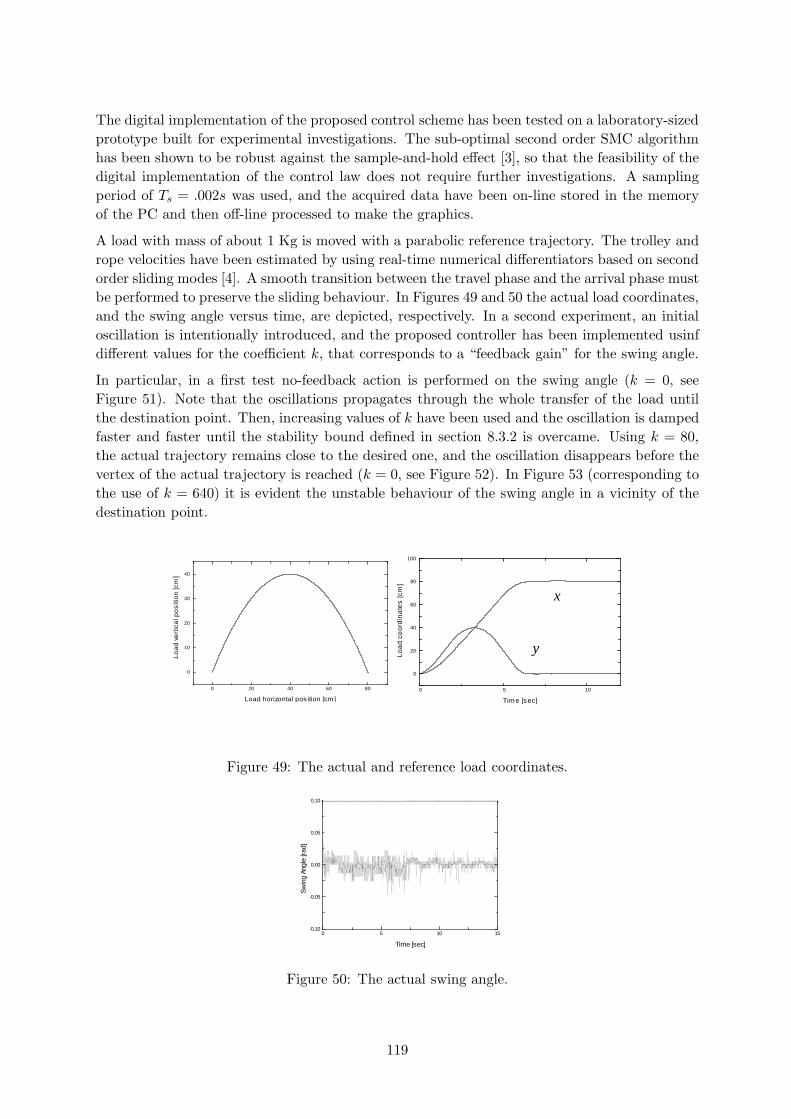
In the Part II the control problems of robotic manipulators, induction motors and overhead

container cranes are addressed and solved, using the 2-sliding mode approach, in Chapters 6, 7

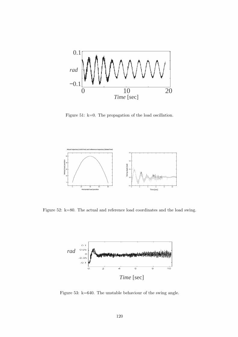
and 8 respectively.

4

Introduction and Motivations

In recent years the availability of powerful low-cost microprocessors has made actually imple-

mentable complex, and very efficient, nonlinear control strategies.

In particular, motivated by a large amount of important practical problems, the control of un-

certain nonlinear systems has become an important subject of research. As a result, considerable

progresses in nonlinear robust control techniques, such as nonlinear adaptive control, geometric-

approach based control, backstepping, sliding mode control and others, that explicitly account

for an imprecise description of the model of the controlled plant, guaranteeing the attainment

of the relevant control objectives in the face of modeling error and/or parameter uncertainties,

have been attained.

Sliding mode control is generally recognized as very robust and simple to implement, but the

so-called “ chattering phenomenon” (the effects of the discontinuous nature of the control), and

the high control activity, have originated a certain skepticism about such an approach.

This work analyzes a quite recent development of sliding mode control, namely the second

order sliding mode approach, which is encountering a growing attention in the control research

community.

The objective of this thesis is to survey the theoretical background of the second order sliding

mode control, mainly developed in the last years, to present some new results, and to show that

the second order sliding mode approach, is an effective solution to the above-cited drawbacks,

and may constitute a good candidate for solving a wide range of important practical problems.

5

Part I

Theory

6

1 Variable Structure Systems and Sliding Modes

1.1 Preliminaries

This work deals with a special class of systems, called “VARIABLE STRUCTURE SYSTEMS”

(VSSs), that are of great importance in systems and control theory.

The concept of VSS, and its applications to the control theory, were originated mainly by the

work of researchers from the former Russia, starting from the sixties [Emel’yanov and Taran ‘62,

Emel’yanov ed ‘70, Utkin ‘78, Ytkis ‘92]. Nowadays, the VSS theory involves a wide research

community, and it is one of the most promising control methodologies [Young et al. 1999,

Young et al. 1999, Utkin ‘00].

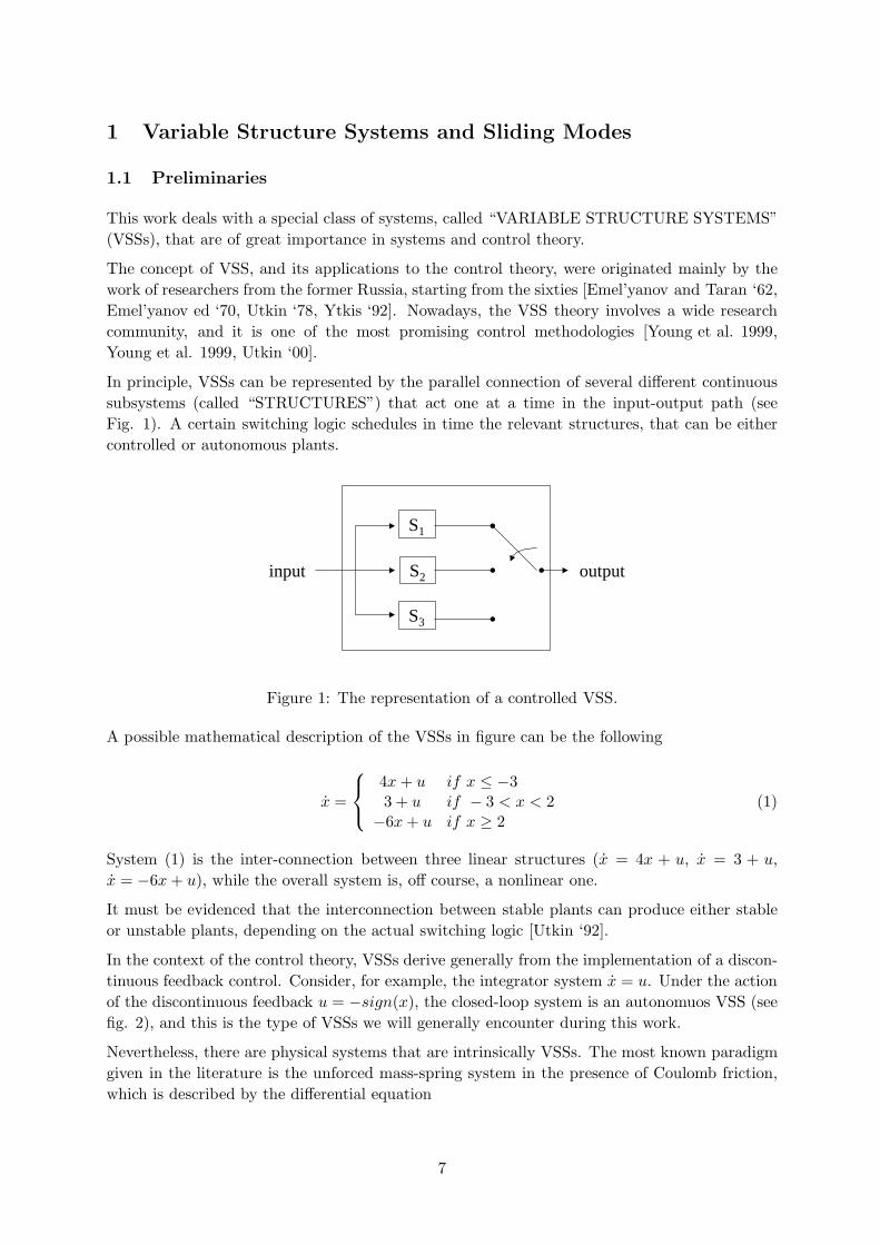
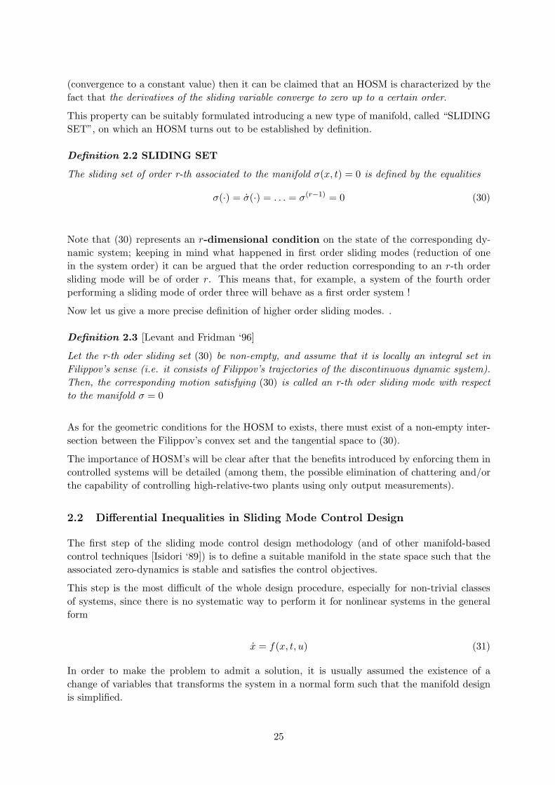
In principle, VSSs can be represented by the parallel connection of several different continuous

subsystems (called “STRUCTURES”) that act one at a time in the input-output path (see

Fig. 1). A certain switching logic schedules in time the relevant structures, that can be either

controlled or autonomous plants.

S1

S2

S3

input output

Figure 1: The representation of a controlled VSS.

A possible mathematical description of the VSSs in figure can be the following

x =

4x+ u if x ≤ −33 + u if − 3 < x < 2

−6x+ u if x ≥ 2(1)

System (1) is the inter-connection between three linear structures (x = 4x + u, x = 3 + u,

x = −6x+ u), while the overall system is, off course, a nonlinear one.

It must be evidenced that the interconnection between stable plants can produce either stable

or unstable plants, depending on the actual switching logic [Utkin ‘92].

In the context of the control theory, VSSs derive generally from the implementation of a discon-

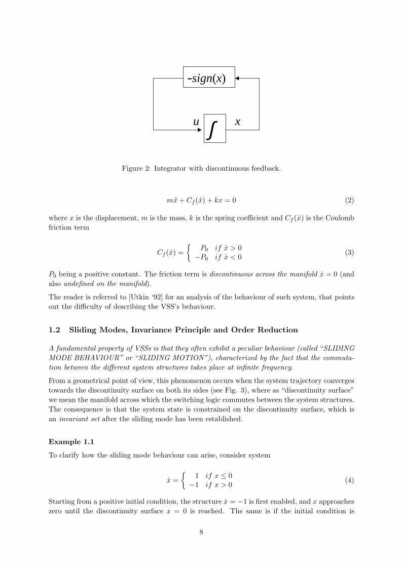
tinuous feedback control. Consider, for example, the integrator system x = u. Under the action

of the discontinuous feedback u = −sign(x), the closed-loop system is an autonomuos VSS (see

fig. 2), and this is the type of VSSs we will generally encounter during this work.

Nevertheless, there are physical systems that are intrinsically VSSs. The most known paradigm

given in the literature is the unforced mass-spring system in the presence of Coulomb friction,

which is described by the differential equation

7

-sign(x)

xu ∫

Figure 2: Integrator with discontinuous feedback.

mx+ Cf (x) + kx = 0 (2)

where x is the displacement, m is the mass, k is the spring coefficient and Cf (x) is the Coulomb

friction term

Cf (x) =

P0 if x > 0−P0 if x < 0

(3)

P0 being a positive constant. The friction term is discontinuous across the manifold x = 0 (and

also undefined on the manifold).

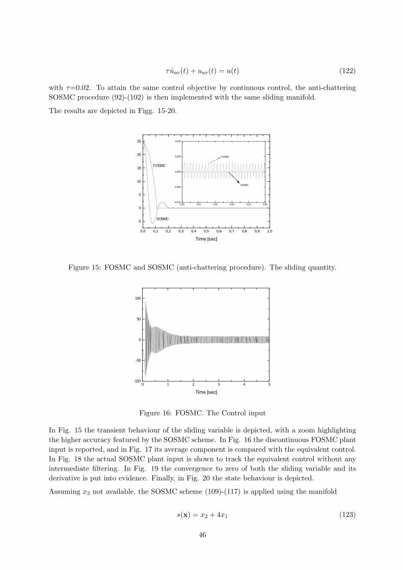
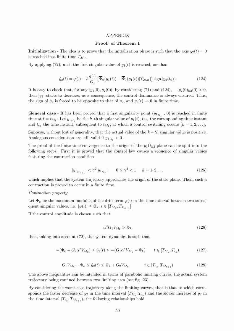
The reader is referred to [Utkin ‘92] for an analysis of the behaviour of such system, that points

out the difficulty of describing the VSS’s behaviour.

1.2 Sliding Modes, Invariance Principle and Order Reduction

A fundamental property of VSSs is that they often exhibit a peculiar behaviour (called “SLIDING

MODE BEHAVIOUR” or “SLIDING MOTION”), characterized by the fact that the commuta-

tion between the different system structures takes place at infinite frequency.

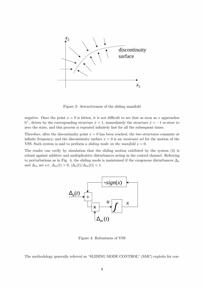
From a geometrical point of view, this phenomenon occurs when the system trajectory converges

towards the discontinuity surface on both its sides (see Fig. 3), where as “discontinuity surface”

we mean the manifold across which the switching logic commutes between the system structures.

The consequence is that the system state is constrained on the discontinuity surface, which is

an invariant set after the sliding mode has been established.

Example 1.1

To clarify how the sliding mode behaviour can arise, consider system

x =

1 if x ≤ 0−1 if x > 0

(4)

Starting from a positive initial condition, the structure x = −1 is first enabled, and x approaches

zero until the discontinuity surface x = 0 is reached. The same is if the initial condition is

8

discontinuitysurface

x1

x2

Figure 3: Attractiveness of the sliding manifold

negative. Once the point x = 0 is hitten, it is not difficult to see that as soon as x approaches

0+, driven by the corresponding structure x = 1, immediately the structure x = −1 re-steer to

zero the state, and this process is repeated infinitely fast for all the subsequent times.

Therefore, after the discontinuity point x = 0 has been reached, the two structures commute at

infinite frequency, and the discontinuity surface x = 0 is an invariant set for the motion of the

VSS. Such system is said to perform a sliding mode on the manifold x = 0.

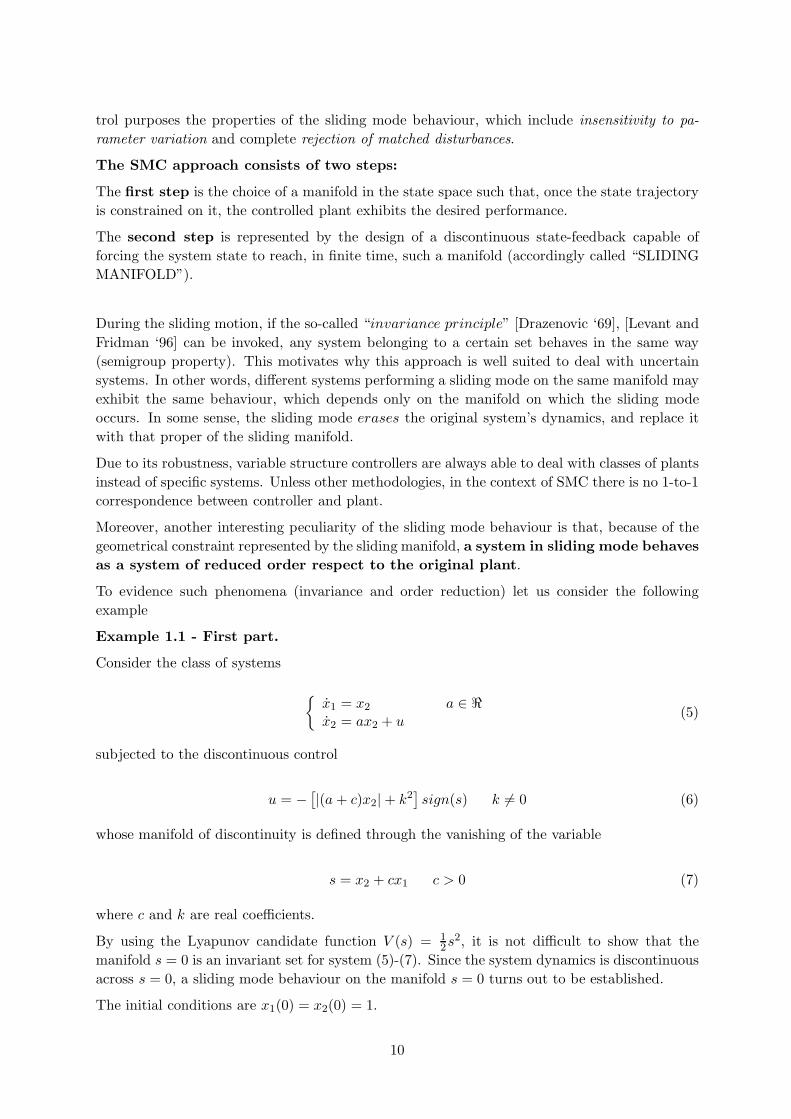
The reader can verify by simulation that the sliding motion exhibited by the system (4) is

robust against additive and multiplicative disturbances acting in the control channel. Referring

to perturbations as in Fig. 4, the sliding mode is maintained if the exogenous disturbances ∆a

and ∆m are s.t. ∆m(t) > 0, |∆a(t)/∆m(t)| < 1.

-sign(x)

xu∫

+∆a(t)

×

∆m (t)

Figure 4: Robustness of VSS

The methodology generally referred as “SLIDING MODE CONTROL” (SMC) exploits for con-

9

trol purposes the properties of the sliding mode behaviour, which include insensitivity to pa-

rameter variation and complete rejection of matched disturbances.

The SMC approach consists of two steps:

The first step is the choice of a manifold in the state space such that, once the state trajectory

is constrained on it, the controlled plant exhibits the desired performance.

The second step is represented by the design of a discontinuous state-feedback capable of

forcing the system state to reach, in finite time, such a manifold (accordingly called “SLIDING

MANIFOLD”).

During the sliding motion, if the so-called “invariance principle” [Drazenovic ‘69], [Levant and

Fridman ‘96] can be invoked, any system belonging to a certain set behaves in the same way

(semigroup property). This motivates why this approach is well suited to deal with uncertain

systems. In other words, different systems performing a sliding mode on the same manifold may

exhibit the same behaviour, which depends only on the manifold on which the sliding mode

occurs. In some sense, the sliding mode erases the original system’s dynamics, and replace it

with that proper of the sliding manifold.

Due to its robustness, variable structure controllers are always able to deal with classes of plants

instead of specific systems. Unless other methodologies, in the context of SMC there is no 1-to-1

correspondence between controller and plant.

Moreover, another interesting peculiarity of the sliding mode behaviour is that, because of the

geometrical constraint represented by the sliding manifold, a system in sliding mode behaves

as a system of reduced order respect to the original plant.

To evidence such phenomena (invariance and order reduction) let us consider the following

example

Example 1.1 - First part.

Consider the class of systems

x1 = x2 a ∈ ℜx2 = ax2 + u

(5)

subjected to the discontinuous control

u = −[

|(a+ c)x2| + k2]

sign(s) k 6= 0 (6)

whose manifold of discontinuity is defined through the vanishing of the variable

s = x2 + cx1 c > 0 (7)

where c and k are real coefficients.

By using the Lyapunov candidate function V (s) = 12s

2, it is not difficult to show that the

manifold s = 0 is an invariant set for system (5)-(7). Since the system dynamics is discontinuous

across s = 0, a sliding mode behaviour on the manifold s = 0 turns out to be established.

The initial conditions are x1(0) = x2(0) = 1.

10

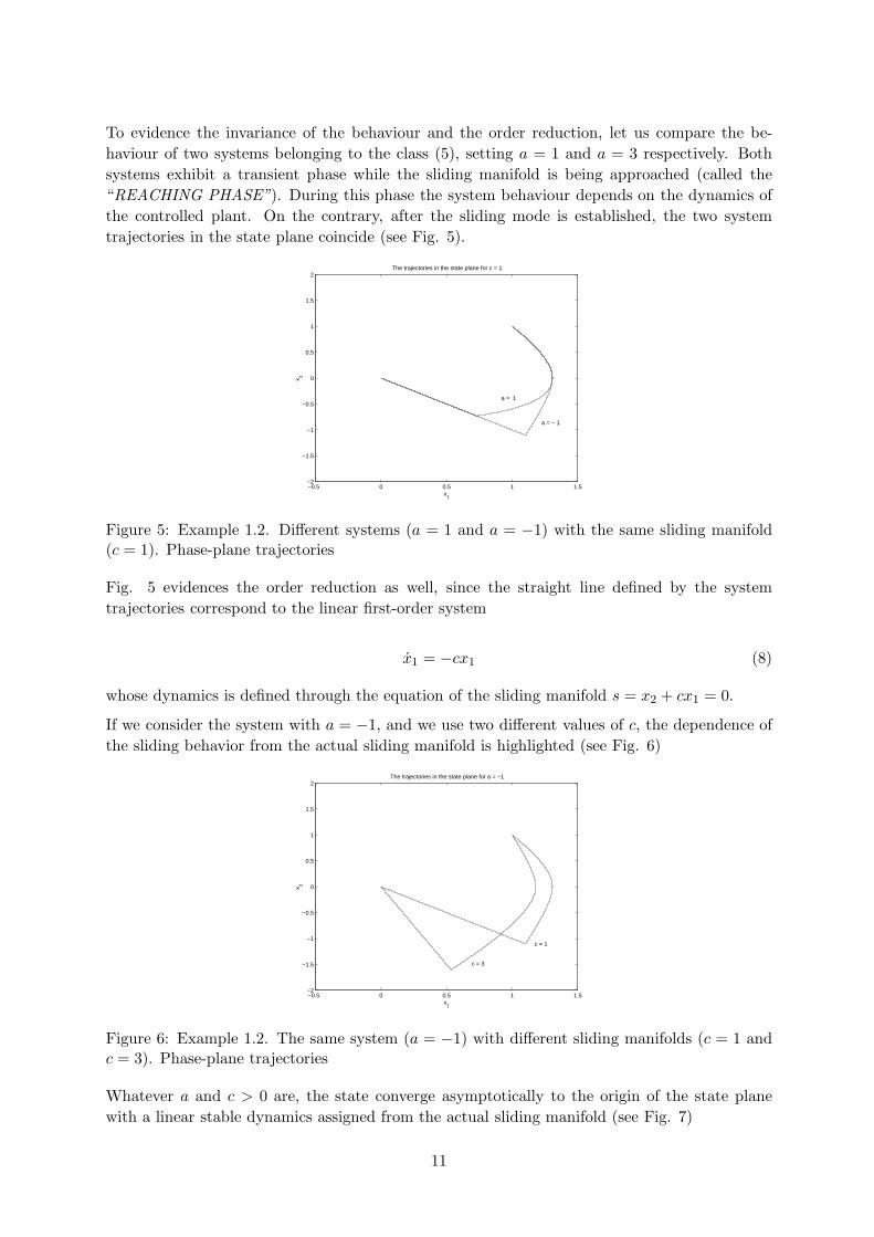
To evidence the invariance of the behaviour and the order reduction, let us compare the be-

haviour of two systems belonging to the class (5), setting a = 1 and a = 3 respectively. Both

systems exhibit a transient phase while the sliding manifold is being approached (called the

“REACHING PHASE”). During this phase the system behaviour depends on the dynamics of

the controlled plant. On the contrary, after the sliding mode is established, the two system

trajectories in the state plane coincide (see Fig. 5).

−0.5 0 0.5 1 1.5−2

−1.5

−1

−0.5

0

0.5

1

1.5

2

x1

The trajectories in the state plane for c = 1

x 2

a = − 1

a = 1

Figure 5: Example 1.2. Different systems (a = 1 and a = −1) with the same sliding manifold(c = 1). Phase-plane trajectories

Fig. 5 evidences the order reduction as well, since the straight line defined by the system

trajectories correspond to the linear first-order system

x1 = −cx1 (8)

whose dynamics is defined through the equation of the sliding manifold s = x2 + cx1 = 0.

If we consider the system with a = −1, and we use two different values of c, the dependence of

the sliding behavior from the actual sliding manifold is highlighted (see Fig. 6)

−0.5 0 0.5 1 1.5−2

−1.5

−1

−0.5

0

0.5

1

1.5

2

x1

x 2

The trajectories in the state plane for a = −1

c = 3

c = 1

Figure 6: Example 1.2. The same system (a = −1) with different sliding manifolds (c = 1 andc = 3). Phase-plane trajectories

Whatever a and c > 0 are, the state converge asymptotically to the origin of the state plane

with a linear stable dynamics assigned from the actual sliding manifold (see Fig. 7)

11

0 1 2 3 4 5 6 7 8 9 10−2

−1.5

−1

−0.5

0

0.5

1

1.5

Time [sec]

x 1(t)

− x

2(t)

The state variables vs time

x1(t)

x2(t)

Figure 7: Example 1.2. The state trajectories vs time for a = −1, c = 3 and k2 = 1

The robust convergence to zero of the state vector components encountered has not a general

validity, and it is due, in the above example, to the chain-of-integrators normal form of system

(5)-(7). More general classes of systems, even in sliding mode on the same manifold, could be

unstable. The reader can easily verify through simulation that the system

x1 = x2 + bx21 a, b ∈ ℜ

x2 = ax2 + u(9)

with a feedback control

u = −[

|(a+ c)x2| + |bc|x21k

2]

sign(s) (10)

evolves in sliding mode on the manifold x2 + cx1 = 0 and its state variables may escape to

infinity (in finite time !) if the initial conditions are not sufficiently close to zero (set, for

example, k2 = c = a = 1 and x1(0) = 2, x2(0) = −2).

The analysis of the behaviour of non-trivial classes of VSSs (borrowing the terminology intro-

duced by Isidori [Isidori ‘89], we can refer to the sliding mode dynamics as the “zero dynamics

respect to the output variable s”) is a challenging task. The next subsection is devoted to give

some fundamental results about this topic, and the unstable behaviour of system (9)-(10) will

be justified.

1.3 VSS Analysis. The Filippov continuation method and the equivalent

control method.

If some uncertainties affect the description of the controlled system, as always happens in real-

life application, it is worth noting that a control ensuring the fulfillment of the ideal sliding

mode objective is intrinsically discontinuous and with infinite switching frequency, having to

instantaneously react to any deviation of the system trajectory from the sliding manifold.

The following question arises spontaneously:

12

“What’s the behaviour of a dynamical system subjected to a discontinuous control action char-

acterized by infinite switching frequency?”

In other words: how to define the system trajectories during a sliding mode on a manifold ?

The reply is not straightforward, neither from a mathematical point of view nor from a “

practical” one, since the VSS behaviour is quite far from the typical one to which the control

engineer is get used (except from few exceptions, alike electrical engineers involved in PWM-

based power electronics applications).

The problem of the VSS analysis leads to the solution of a differential equation with discontinuous

right-hand side, that was first addressed and solved in the sixties by the Russian mathematician

Filippov, in a purely mathematical framework of research [Filippov ‘88]

More precisely, consider the dynamic system

x = f(x, t,u) x ∈ Rn u ∈ Rm (11)

subjected to the discontinuous feedback

ui =

u+i (x, t) if si(x, t) > 0u−i (x, t) if si(x, t) < 0

i = 1, 2, . . . ,m (12)

where u=[u1(x, t), u2(x, t), . . . , um(x, t)]T .

Under suitable assumptions, the closed-loop system (11)-(12) may exhibit a sliding behaviour

on the m-dimensional manifold s(x, t) = 0, where s=[s1(x, t), s2(x, t),. . . , sm(x, t)]T

The regularity assumptions that ensure the existence of a solution in the classical sense are not

verified on the discontinuity manifold s = 0.

Skipping more complex technicalities (for which the reader is referred to [Filippov ‘88] and, for

shorter discussions, to [Utkin ‘92, Levant ‘93]), Filippov demonstrated that the solution of the

equation (11),(12) onto the discontinuity surface satisfies the differential inclusion

x ∈ V (x, t) (13)

where the set V (x, t) is the minimal convex closure containing all values of f(x, t,u(x, t)) when

x covers the entire δ-neighbourhood of the manifold (possibly except from a zero-measure set).

Once defined the set V (x, t), the velocity vector f0(x, t) describing the sliding mode behaviour

is taken, within the set V (x, t), as that tangent to the manifold of discontinuity.

The above-defined solution is called “solution in the Filippov sense”.

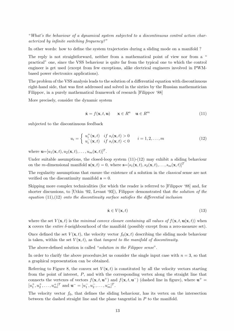
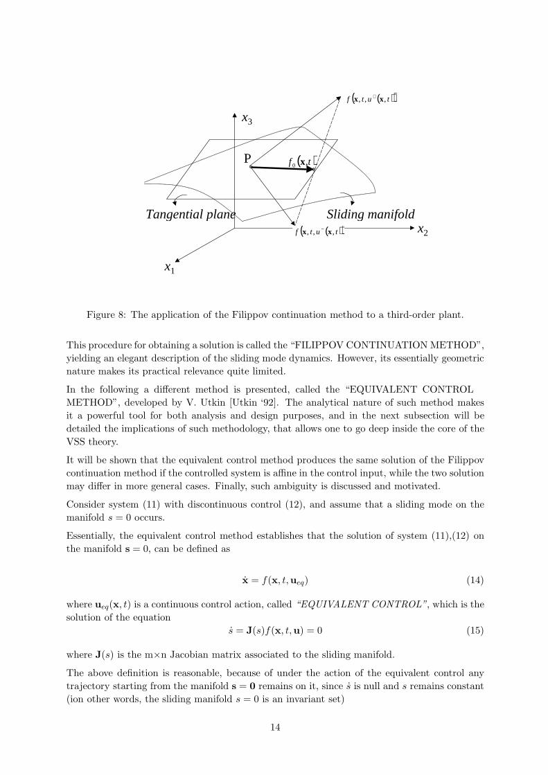
In order to clarify the above procedure,let us consider the single input case with n = 3, so that

a graphical representation can be obtained.

Referring to Figure 8, the convex set V (x, t) is constituted by all the velocity vectors starting

from the point of interest, P , and with the corresponding vertex along the straight line that

connects the vertexes of vectors f(x, t,u+) and f(x, t,u−) (dashed line in figure), where u+ =

[u+1 , u

+2 , . . . , u

+m]T and u− = [u−1 , u

−2 , . . . , u

−m]T .

The velocity vector f0, that defines the sliding behaviour, has its vertex on the intersection

between the dashed straight line and the plane tangential in P to the manifold.

13

Sliding manifoldTangential plane

P

( )( )tutf ,,, xx +

( )( )tutf ,,, xx −

( ),tf x0

x2

x1

x3

Figure 8: The application of the Filippov continuation method to a third-order plant.

This procedure for obtaining a solution is called the “FILIPPOV CONTINUATION METHOD”,

yielding an elegant description of the sliding mode dynamics. However, its essentially geometric

nature makes its practical relevance quite limited.

In the following a different method is presented, called the “EQUIVALENT CONTROL

METHOD”, developed by V. Utkin [Utkin ‘92]. The analytical nature of such method makes

it a powerful tool for both analysis and design purposes, and in the next subsection will be

detailed the implications of such methodology, that allows one to go deep inside the core of the

VSS theory.

It will be shown that the equivalent control method produces the same solution of the Filippov

continuation method if the controlled system is affine in the control input, while the two solution

may differ in more general cases. Finally, such ambiguity is discussed and motivated.

Consider system (11) with discontinuous control (12), and assume that a sliding mode on the

manifold s = 0 occurs.

Essentially, the equivalent control method establishes that the solution of system (11),(12) on

the manifold s = 0, can be defined as

x = f(x, t,ueq) (14)

where ueq(x, t) is a continuous control action, called “EQUIVALENT CONTROL”, which is the

solution of the equation

s = J(s)f(x, t,u) = 0 (15)

where J(s) is the m×n Jacobian matrix associated to the sliding manifold.

The above definition is reasonable, because of under the action of the equivalent control any

trajectory starting from the manifold s = 0 remains on it, since s is null and s remains constant

(ion other words, the sliding manifold s = 0 is an invariant set)

14

Example 1.1 - Second part.

Let us analyze the behaviour of systems (5)-(6) and (9)-(10), both in sliding mode on the

manifold s = x2 + cx1 = 0.

Simulations results have shown that the state of the first system exhibit a stable behaviour,

while the state of the second one escapes to infinity (in finite time!). Now we are able to justify

the reasons for this difference.

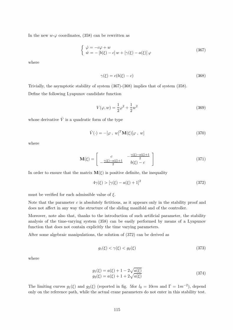
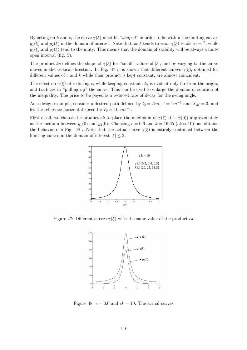
As for system (5)-(6), applying the definition of the equivalent control yields

s = x2 + cx2 = ax2 + u+ cx2 = 0 ⇐⇒ u = ueq = −(a+ c)x2 (16)

Substituting ueq for u in the last equation of (5) one obtains

x2 = −cx2 (17)

Taking into account that x2 = −cx1, the dynamics of x1 is stable as well.

Repeating the same procedure for system (9), one has

s = x2 + cx2 = ax2 + u+ cx2 + bcx21 (18)

and the equivalent control turns out to be given by

ueq = −(a+ c)x2 − bcx21 (19)

which, substituted in (9), after some manipulations, leads to

x2 = −cx2 −b

cx2

2 (20)

which may be either stable or unstable depending on the initial condition.

From a geometrical point of view, the vertex of the velocity vector f(x, t,ueq) is obtained

intersecting the tangential plane with the locus of f(x, t,u) for u varying between u− and u+.

In the following figure 9, the equivalent control method is applied to a second-oder single-input

system. The locus of f(x, t,u) is the dashed line, and its intersection with the straight line

tangential to the manifold defines the vertex of the velocity vector f(x, t,ueq) that describes the

sliding mode behaviour.

It is apparent that the solution found by means of the equivalent control method is generally

different from that obtained using the Filippov method. This is highlighted by analyzing the

following figure 10, in which it is also described the very particular case in which the intersection

occurs in the same point (locus of type B) and the two solutions coincide. In this latter case,

f0(x, t) ≡ f(x, t,ueq) would be the unambiguous solution to the problem.

It must be evidenced that there exists an important class of systems for which both the methods

of analysis lead to the same solution. Such class is that of the the systems with affine dependance

on the control, i.e. systems expressed as follows

15

( )+utf ,,x

( )−utf ,,x

( ) ,, utfoflocus x

( )equtf ,,x

x1

x2

The sliding manifold

The tangential line

Figure 9: The application of the equivalent control method to a second-order plant.

( )+utf ,,x

( )−utf ,,x

A locus

( )eqA utf ,,x( )tf ,0 x

Blocus

x1

x2

Figure 10: Comparison between the Filippov method and the equivalent control method.

x = a(x, t) + b(x, t)u x ∈ Rn u ∈ Rm (21)

Indeed, in this case, it is easy to see that the locus of f(x, t,u)(, a(x, t) + b(x, t)u) coincides

with the above defined minimal convex set V (x, t), and the correspondence of the solutions is

the trivial consequence.

Some comments are needed about the non-uniqueness of the solution in the general case of

nonlinear systems with arbitrary dependence on the control.

The conceptual difference between the two methods is that the Filippov method prescinds from

the existence of a control action able to generate the velocity vector f0(x, t).

The equivalent control, on the contrary, searches the solution only within the “feasible set” of

velocity vector, i.e. there always exists a continuous control action that represents (“is equivalent

to”) the discontinuous control.

This difference originates a different capability of the two methods to capture the plant be-

haviour. In fact, it is noteworthy that a discontinuous infinite-frequency switching signal is

16

physically meaningless, so that in real applications must be replaced by some approximation.

The Filippov method is devoted to deal with cases in which the actual control is discontinuous

in a neighbour of the sliding manifold (i.e. when the switching control is implemented by means

of a switch with an hysteresis).

On the other hand, the equivalent control method is well suited when the control law is imple-

mented by means of continuous approximations of the sign function, i.e. when the motion in a

neighbour of the manifold is smooth.

Summarizing, when the sliding mode behaviour of a system nonlinear in the control law is

investigated, there is no ”correct” or ”uncorrect” solution, but the right way to understand the

system behaviour depends on the actual implementation of the control law [Utkin ‘92].

1.4 Ideal and Real Sliding. Chattering, Identificability and Approximability.

In real-life applications, it is not reasonable to assume that the control signal time evolution can

switch at infinite frequency, while it is more realistic, due to the inertias of the actuating and

measuring devices, and to the presence of noise and/or exogenous disturbances, to assume that

it commute at a very high (but finite) frequency. The control oscillation frequency turns out to

be not only finite but also almost unpredictable.

The main consequence is that the sliding mode takes place in a small neighbour of the sliding

manifold, whose dimension is inversely proportional to the control switching frequency.

We introduce the notions of “IDEAL SLIDING MODE” and “REAL SLIDING MODE” to

distinguish the sliding motion that occurs exactly on the sliding manifold (analyzed in previous

subsections assuming ideal control devices) from a sliding motion that, due to the non-idealities

of the control law implementation, takes place in a vicinity of the sliding manifold, which is

called “BOUNDARY LAYER”.

The effects of the finite switching frequency of the control are referred in the literature as

“CHATTERING”. Basically, the high frequency components of the control propagate through

the system, therefore exciting the unmodeled fast dynamics, and undesired oscillations affect the

system output. Moreover, the term “chattering” has been also designated to indicate the bad

effect, potentially disruptive, that a switching control force/torque can produce on the controlled

mechanical plant.

Chattering and high control activity were the major drawbacks of the sliding mode approach in

the practical realization of variable structure control (VSC) schemes [Utkin ‘92] [DeCarlo et al.

‘88].

In order to overcame these drawbacks, a research activity aimed at finding a continuous control

action, robust against uncertainties and disturbances, guaranteeing the attainment of the same

control objective of the standard sliding mode approach has been carried out in recent years

[Bartolini et al. ‘96, Bartolini et al. ‘98b, Sira-Ramirez ‘92].

A possible way to reduce chattering, though maintaining a very high switching frequency, is

based on the use of observers for the modeled part of the system [Utkin ‘92]. The sliding

mode is generated in the observer state space with a motion which is close to the ideal one.

The resulting high frequency control is filtered out by the fast dynamics of the plant so that a

practical continuous control is fed to the slow dynamical subsystem (see Fig. 11). This approach,

in the case of known nonlinear systems, has been proposed in [Sira-Ramirez ‘92], while it has

17

been extended to uncertain systems in [Bartolini et al. ‘96].

System

( ) ( )ugf xxx += cxs(x)x(t)uη

sign(⋅)X

η

t

u

t

s

t

-

Observer

( )tx

( )txcˆ( )xs +

t

s

H(t)

Unmodeleddynamics

( )η,xhu =

Figure 11: Elimination of chattering via the use of asymptotic observers

Another approach, probably the most used in practice, is based on the use of continuous ap-

proximations of the sign function (such as the sat(·) function, the tanh(·) function and so on)

in the implementation of the control law. It was pointed out in [Slotine and Li ‘91] as this

methodology is highly sensitive to the unmodeled fast dynamics, and in some cases can lead

to unacceptable performance. An interesting class of smoothing functions, characterized by a

time-varying parameters, was proposed in [Slotine and Li ‘91], attempting to find a compromise

between the chattering elimination aim and the possible excitation of the unmodeled dynamics.

The most recent and interesting approach for the elimination of chattering is represented (at least

in the authors’ opinion) by the second order sliding mode methodology, that will be extensively

detailed in the following of the present thesis.

1.4.1 Identificability: the on-line availability of the equivalent control

The invariance property establishes that different systems may exhibit the same behaviour when

constrained to evolve on the same manifold.

Although any informations regarding the original plant seem to be “lost” during the sliding mo-

tion, V. Utkin theorized the possibility of recovering it through the analysis of the discontinuous

plant input signal.

He observed that the response of a dynamic system is largely determined by the slow components

of its input, while the fast components are often negligible. On the other hand, the equivalent

control method requires the substitution of the actual discontinuous control with a continuous

function which does not contain high-rate components.

On the basis of the above considerations, he argued that the equivalent control coincides with

the slow components of the input, and was able to give a formal proof of this statement.

In [Utkin ‘92], Utkin succeeded in proving that, under certain assumptions on the system dy-

namics, if the system remains within a ∆-vicinity of the sliding manifold, the output of the

first-order filter

18

τ uav(t) + uav(t) = u(t) (22)

where u is the actual control input, is close to the equivalent control according to the following

inequality

|uav(t) − ueq(t)| ≤ k0|uav(0) − ueq(0)|e−t/τ + k1τ + k2∆ + k3∆

τ(23)

where k0, k1, k2, k3 are proper known constants.

This result is not valid for systems nonlinear in the control law, as in such systems the dynamic

plant response to the high-frequency terms cannot generally be neglected.

The expression (23) contains useful informations on the criterion for properly choosing the filter

time constant τ in order to achieve the best estimate.

It is apparent that the right-hand side of (23) can be minimized if the time constant τ of the

filter is taken to be proportional to√

∆, which leads to

|uav(t) − ueq(t)| ≤ O(√

∆)

(24)

The filter time constant, that must be small enough as compared with the slow components

of the control yet large enough to filter out the high-rate components, is to be chosen suitably

matched with the size of the boundary layer.

This property of “identificability” constitutes one of the most important structural property

of sliding mode control. It has been successfully applied for design purposes in various works

[Hsu et al.‘89, Fu et al. ‘91], and also has been recently extended to the second order sliding

mode control setting [Bartolini et al. ‘98a].

1.4.2 The Approximability Property

To validate the application of the sliding mode control methodology, which always gives rise to

sliding modes on some vicinities of the relevant sliding manifold, it is crucial to understand if

the description of the sliding mode behaviour is regular respect to small deviations from the

manifold.

In other terms, are the real sliding mode trajectories close to the ideal ones obtained through

the methods in Subsect. 1.3?

A first reply is contained in a fundamental Theorem, demonstrated in [Utkin ‘92], that basically

states that under reasonable smoothness assumptions on the system dynamics, the above reg-

ularity property (called “ APPROXIMABILITY PROPERTY”) always holds in systems affine

in the control.

The Utkin’s Theorem sounds like follows:

Under certain assumptions there exists a constant M such that, for any ∆ ≥ 0, the following

correspondance occurs

19

‖s(t)‖ ≤ ∆ ⇐⇒ ‖x(t) − x∗(t)‖ ≤M∆ (25)

where s is the sliding variable, and x(t), x∗(t) are the system trajectories in real and ideal sliding

mode respecticively

The analysis of the approximability for systems non-affine in the control law has been pioneered

in [Bartolini et al. ‘86]. For more details the reader is referred to the above work (and references

therein).

1.5 Considerations

The main advantages of the SMC approach are the simplicity (of both design and implemen-

tation), the high efficiency and the robustness. The basic properties are the order reduction,

invariance principle and approximability.

Chattering and high control activity were the reasons that fomented a generalized criticism

towards SMC. Nowadays, due to great advances in the research, a number of effective SMC-based

control tools is available for practicing engineers that must address complex control problems

involving nonlinearities and/or hard uncertainties [Young et al. 1999]

In the second part of this thesis, in which some applicative problems are addressed and solved

by second order sliding mode technique, the superb theoretical properties of SMC are confirmed

in applications.

Some performance indexes to compare different sliding mode control strategies could be the

real ACCURACY in implementation, the smoothness of the control law and the information

demand. On the basis of all this criteria, second order sliding mode control reveals itself as an

improvement respect to previous methodologies.

It is the objective of this thesis to detail a collection of tools, based on second order sliding

modes, whose effectiveness cover a large number of practical cases, ranging from discrete-time

(or sampled-data) systems to continuous ones, and encompassing important physical plants

(even underactuated, see Chapter 8), hoping that this work will attract attention (as well as

stimulate experimental activities) about this novel class of algorithms.

References

[Drazenovic ‘69] B. Drazenovic, “The invariance condition in variable structure systems”, Auto-

matica, vol. 5, pp. 287–295, 1969.

[Bartolini et al. ‘86] G. Bartolini and T. Zolezzi, “Control of Nonlinear Variable Structure Sys-

tems”, J. Math. Analysis Appl., vol.118, pp. 42–62, 1986.

[Bartolini et al. ‘96] G. Bartolini, P. Pydynowski, “An improved chattering free VSC scheme for

uncertain dynamical systems”, IEEE Trans. on Automatic Control, vol. 41, pp. 1220–1226,

1996.

20

[Bartolini et al. ‘97] G. Bartolini, A. Ferrara, E. Usai, “Applications of a sub–optimal discontin-

uous control algorithm for uncertain second order systems”, Int. J. of Robust and Nonlinear

Control, vol. 7, no.4, pp. 299–319, 1997.

[Bartolini et al. ‘98a] G. Bartolini, A. Ferrara, A. Pisano and E. Usai “Adaptive reduction of the

control effort in chattering-free sliding mode control of uncertain nonlinear plants”, J. Appl.

Math. and Comp. Sc., vol. 8, no. 1, pp. 51–71, 1998.

[Bartolini et al. ‘98b] G. Bartolini, A. Ferrara, E. Usai, “Chattering Avoidance by Second Order

Sliding Mode Control”, IEEE Trans. on Automatic Control, vol. 43, no. 2, pp. 241–246, 1998.

[DeCarlo et al. ‘88] R.A. De Carlo, S.H. Zak, G.P. Matthews “Variable Structure Control of

Nonlinear Multivariable Systems: A Tutorial”, Proceedings of the IEEE, vol. 76, no. 3, pp.

212–232, 1988.

[Emel’yanov and Taran ‘62] S.V. Emel’yanov and V.A. Taran “On a class of Variable Structure

Control Systems ”, Proc. of USSR Academy of Sciences, Energy and Automation, No. 3, 1962

(in russian).

[Emel’yanov ed ‘70] “Theory of Variable Structure Systems ”, S.V. Emel’yanov ed., Nauka,

Moscow, 1970 (in russian).

[Fu et al. ‘91] L.C. Fu, “A robust model reference adaptive control using variable structure adap-

tation for a class of plants”, Int. J. Contr., vol.53, pp. 1359–1375, 1991.

[Hsu et al.‘89] L. Hsu and R.R. Costa “Variable structure model reference adaptive control using

only input and output measurement: Part 1 ”, Int. J. Contr., vol.49, no. 2, pp. 399–419, 1989.

[Filippov ‘88] A.F. Filippov Differential Equations with Discontinuous Right–Hand Side, Kluwer,

Dordrecht, Netherlands, 1988.

[Isidori ‘89] A. Isidori Non Linear Control Systems, Springer Verlag, Berlin, 1989.

[Levant ‘93] A. Levant “Sliding order and sliding accuracy in sliding mode control”, International

Journal of Control, vol. 58, pp. 1247–1263, 1993.

[Levant and Fridman ‘96] A. Levant, L. Fridman “Higher order sliding modes as a natural phe-

nomenon in control theory” in Robust control via variable structure and Lyapunov techniques,

F. Garofalo and L. Glielmo Eds., Lecture Notes in Control and Information Sciences, vol.

217, pp. 107–133, Springer–Verlag, London, 1996.

[Sira-Ramirez ‘92] H. Sira–Ramirez “On the sliding mode control of nonlinear systems,” Syst.

Contr. Lett., vol. 19, pp. 303–312, 1992.

[Slotine and Li ‘91] J.J.E.Slotine, W. Li Applied Nonlinear Control, Prentice–Hall International,

Englewood Cliffs, New Jersey, 1991.

[Utkin ‘78] V.I. Utkin Sliding Modes and their Applications in Variable Structure Systems, Mir,

Moscow, 1978 (in russian).

[Utkin ‘92] V.I. Utkin Sliding Modes in Control and Optimization, Springer Verlag, Berlin, 1992.

[Utkin ‘99] V.I. Utkin et al. Sliding Modes Control in Electromechanical Systems, Taylor and

Francis, London, 1999.

21

[Utkin ‘00] V.I. Utkin “VSS Premise in XX Century: Evidence of a Witness”, Proc. of the 6th

IEEE Int. Workshop on Variable Structure Systems, Coolangatta, Australia, Dec. 2000, pp.

1- 32.

[Young and Ozguner eds., ‘99] K.D. Young and U. Ozguner (eds.)“Variable Structure Systems,

Sliding Mode and Nonlinear Control”, Lecture Notes in Control and Information Sciences,

Springer-Verlag, 1999, in press.

[Young et al. 1999] D. Young, U. Ozguner and V. Utkin, “A control engineers guide to sliding

mode control”, IEEE Trans. Contr. Syst. Tech., vol 7, pp. 328–342, 1999.

[Ytkis ‘92] U. Ytkis Control Systems of Variable Structure, Wiley, New York, 1976.

[Zinober ‘94] A.S.I. Zinober (Ed.), Variable Structure and Lyapunov Control, Lecture Notes in

Control and Information Sciences, 193, Springer–Verlag, London, 1994.

22

2 Sliding Order in Sliding Mode Control

2.1 Sliding Order and Sliding Sets

We have defined in Chapter 1 a sliding mode on a manifold as a particular type of constrained

motion that is peculiar of variable structure systems. Such a motion is enforced by some dis-

continuity of the system dynamics across the manifold.

The concept of sliding order will be more clear after some considerations about the meaning,

and different types, of “discontinous dynamics” will be given.

It is well known the meaning of the statement “a function f is of class Ck”, i.e. f is continuous

with its derivatives up to the order k. For instance, a function of class C0 is a function whose first

derivative is discontinuous, a function of class C1 is continuous with its first derivative, while

the second one is discontinuous, and so on. In some sense, the class of continuity k represents

the smoothness degree of the corresponding function.

If we try to apply this concept to system motions, instead of considering abstract functions, the

smoothness order of a state trajectory can be defined in a similar manner, keeping in mind that,

due to the own discontinuous nature of variable structure systems’ dynamics, the corresponding

motions are always of finite class Ck.

If the sliding variable σ(x, t) is of class Ck, then the sliding mode on σ(x, t) = 0 is referred as

k − 1-th order sliding mode. Note that the sliding mode of order one corresponds to a sliding

variable of class C0, i.e. with discontinuous derivative. The order of a sliding mode represents

the smoothness degree associated to the motion constrained on the sliding manifold, and it can

be defined as follows

Definition 2.1 The sliding order r is the number of continuous total derivatives (including

the zero one) of the function σ = σ(x, t) whose vanishing defines the equations of the sliding

manifold.

Note that the constrained motions generated by other manifold-based control methodologies

(geometric approach [Isidori ‘89] and others) are generally of infinite smoothness order. More-

over, note also that the sliding order does not depend on the characteristic of the system’s zero

dynamics (i.e. the state behaviour when constrained on the manifold) but it is associated only

to the characteristic of the constrained motion.

REMARK: If we consider the real sliding behaviour (see sect. 1.4), the sliding order establishes,

in some sense, the velocity of the system motion around the sliding manifold. It is not difficult

to argue that the switching imperfections cause the system trajectories to lie on a boundary

layer of the sliding manifold whose size is smaller and smaller as the sliding order increases.

Example 2.1

Consider system

x = u (26)

u = −sign(x) (27)

It has been shown in previous Chapter (see (4)) that the above system exhibits a sliding mode

23

on the manifold σ(x) = x = 0. According to the above definition, such mode is of order one,

because of the total time derivative of the “constraint function” σ, that is given by

σ = x (28)

turns out to be a discontinuous function of the state.

Examples of sliding modes of order higher than one are found in real control systems when some

fast dynamic actuator is used to implement the switching control law [Levant and Fridman ‘96].

Example 2.2

Consider the integrator system, and assume that a dynamic actuator, represented by an high-

bandwidth filter having as its input the switching control, is placed at the input side, i.e.

x = uτu+ u = zz = −sign(x)

(29)

It can be verified that, with sufficiently small τ , a stable sliding mode is established on the

manifold x = 0. Such mode is of order two, as the switching term acts on the second derivative

of the constraint function, and the first total derivative of σ(x) = x is a continuous function of

time.

According to the above remark, one can observe also that the actual size of the residual set to

which x is confined is here much smaller than that attained in Ex 2.1, confirming the higher

real accuracy of second order sliding mode control as compared with first order SMC.

Higher order sliding modes (HOSM) behaviours may occur also when the relative degree r

between the desired constraint function (i.e. the sliding variable) and the control is higher

than one, so that the switching term turns out to be “hidden” in the higher derivatives of the

constraint function. In this case, if the sliding mode is established (a non-trivial control task if

r > 1 !), the sliding order equals the relative degree.

The reader is referred to [Levant and Fridman ‘96] for a detailed discussion about these topics.

Before to give some formal definitions, we try to derive some properties of HOSM from the

analysis of the behaviour of system (29).

Making reference to system (29), one can observe that both x and x are steered to zero.

It isn’t a fortuity, while it is the consequence of a general property of HOSM’s,. that can be

derived through a generalization of the well known Barbalat’s Lemma [Slotine and Li ‘91] (one

of the most important Lemmas in adaptive control), that may be understood as follows:

If some function (signal) converges to a constant value then all its continuous derivatives con-

verge to zero.

On the basis of this very intuitive statement, by combining the above definition of HOSM

(number of continuous derivatives) with the fact that the sliding variable converges to zero

24

(convergence to a constant value) then it can be claimed that an HOSM is characterized by the

fact that the derivatives of the sliding variable converge to zero up to a certain order.

This property can be suitably formulated introducing a new type of manifold, called “SLIDING

SET”, on which an HOSM turns out to be established by definition.

Definition 2.2 SLIDING SET

The sliding set of order r-th associated to the manifold σ(x, t) = 0 is defined by the equalities

σ(·) = σ(·) = . . . = σ(r−1) = 0 (30)

Note that (30) represents an r-dimensional condition on the state of the corresponding dy-

namic system; keeping in mind what happened in first order sliding modes (reduction of one

in the system order) it can be argued that the order reduction corresponding to an r-th order

sliding mode will be of order r. This means that, for example, a system of the fourth order

performing a sliding mode of order three will behave as a first order system !

Now let us give a more precise definition of higher order sliding modes. .

Definition 2.3 [Levant and Fridman ‘96]

Let the r-th oder sliding set (30) be non-empty, and assume that it is locally an integral set in

Filippov’s sense (i.e. it consists of Filippov’s trajectories of the discontinuous dynamic system).

Then, the corresponding motion satisfying (30) is called an r-th oder sliding mode with respect

to the manifold σ = 0

As for the geometric conditions for the HOSM to exists, there must exist of a non-empty inter-

section between the Filippov’s convex set and the tangential space to (30).

The importance of HOSM’s will be clear after that the benefits introduced by enforcing them in

controlled systems will be detailed (among them, the possible elimination of chattering and/or

the capability of controlling high-relative-two plants using only output measurements).

2.2 Differential Inequalities in Sliding Mode Control Design

The first step of the sliding mode control design methodology (and of other manifold-based

control techniques [Isidori ‘89]) is to define a suitable manifold in the state space such that the

associated zero-dynamics is stable and satisfies the control objectives.

This step is the most difficult of the whole design procedure, especially for non-trivial classes

of systems, since there is no systematic way to perform it for nonlinear systems in the general

form

x = f(x, t, u) (31)

In order to make the problem to admit a solution, it is usually assumed the existence of a

change of variables that transforms the system in a normal form such that the manifold design

is simplified.

25

Here we are mainly interested in the second phase, i.e., given a desired manifold σ(x, t) = 0,

whose corresponding zero-dynamics enjoys all properties we can desire, the problem is to find a

control action that forces the system to evolve on such a manifold.

It is shown that the main mathematical tool used for the second step of the SMC design is

constituted by differential inequalities.

In particular, first order SMC is based on differential inequalities of order one, while

second order SMC relies on differential inequalities of order two, much more difficult

to manage.

We consider now for the sake of simplicity systems single-input with affine dependence on the

control, and generalizations are postponed to successive Chapters.

Consider system

x = a(x, t) + b(x, t)u(t) (32)

where x ∈ X is the state variable, X is a smooth finite-dimensional manifold, t is the time,

u ∈ R is the control and a, b are uncertain vector fields.

Let σ(t,x) = 0 be the manifold on which we want to drive the system state. Our goal is to force

the constraint function σ(·) to vanish in finite time.

Using the traditional way to indicate the partial derivatives, σ(t) may be expressed in the form

σ(t) = σ′

t(x, t) + σ′

x(x, t)a(x, t) + σ′

x(x, t)b(x, t)u(t) =

= α(x, t) + β(x, t)u(t)

(33)

where

α(x, t) = σ′

t(x, t) + σ′

x(x, t)a(x, t) (34)

β(x, t) = σ′

x(x, t)b(x, t) (35)

Make the following assumption

A1.

β(x, t) 6= 0 ∀x ∈ X (36)

Assumption A1 means that system (32) has uniform relative degree one with respect to the

output variable σ.

If the system dynamics were perfectly known, the control u(t) could be designed to assign the

desired stable dynamics to the variable σ. Indeed, under suitable minimum-phase assumptions

(stability of the inverse dynamics), the feedback-linearizing control

u(t) = [β(x, t)]−1 [v(t) − α(x, t)] (37)

transforms the expression for σ in the form

26

σ(t) = v(t) (38)

and the signal v(t) may be used to assign the desired dynamics, for instance

v(t) = −kσ(t) k > 0 (39)

would assign a linear first-order stable dynamics to the σ variable.

In the presence of uncertainties, the perfect “cancellation” of the nonlinearities is no more

feasible, and it is not possible to assign a pre-specified dynamics to the σ variable.

At the price of additional assumptions, one can define a control law that makes σ satisfying a

proper differential inequality of order one.

We are interested in differential inequalities whose all possible solutions globally converge to zero.

The most known (and used in control design) is the so-called “REACHING CONDITION”

σσ ≤ k2|σ| (40)

It is not difficult to see that, independently from the initial condition, any solution of (40)

converges to zero in finite time.

If we are able to guarantee that the sliding variable σ satisfies the above condition, then the

finite-time reaching of the sliding manifold turns out to be ensured.

Making reference to (33), we assume that two positive functions αM (x, t) and βm(x, t) exist,

and are known, such that

A2.

|α(x, t)| ≤ αM (x, t) ∀x ∈ X (41)

A3.

0 < βm(x, t) ≤ β(x, t) ∀x ∈ X (42)

The traditional First Order Sliding Mode Control approach is summarized by the following

Proposition, whose proof is trivial and is omitted.

Proposition 2.1 Given the uncertain system (32), satisfying assumptions A2 and A3, then

the feedback control law

u(t) = −αM (x, t) + k2

βm(x, t)sign(σ(x, t)) (43)

provides satisfaction of (40), and therefore, at the same time, the invariance and the global

attractiveness of the manifold σ(x, t) = 0

Basically, in FOSMC the first derivative of the sliding variable is discontinuously modified by

the control signal in order to guarantee that the reaching condition (40), a first-order differential

inequality (FODI) whose solutions globally converge to zero, holds.

27

2.2.1 Second order differential inequalities

As previously mentioned, the second order SMC approach is based on steering σ to zero through

the fulfillment of a differential inequality of order two (second order differential inequality, SODI).

Differential inequalities (DIs) of order higher than one are not trivial to analyze. To apply the

SOSMC methodology, we have first to design a stable SODI, and then a control action must be

found such that the sliding variable σ is forced to satisfy the relevant stable SODI.

It is easy to prove that conditions of the type

σσ ≤ −ξ(t)|σ| ξ(t) ≥ ξ1 > 0 (44)

always give rise to a sequence of singular points

σMi= σ(tMi

) tMi: σ(tMi

) = 0 i = 1, 2, . . . (45)

and, accordingly, to a sequence of time intervals between two successive singular points

∆tMi

=(

tMi+1− tMi

)

(46)

Any possible behaviour of σ, ranging from explosion and persistent oscillations to asymptotic

or finite-time vanishing transients, can arise, depending on the characteristics of the aforesaid

sequences (see Fig. 12)

iMσ

1+iMσ σ

σ

iMσ1+iMσ σ

σ

(a) (b)

σ

Figure 12: Stable and unstable solutions for the SODI (44).

The desired behaviour involves that both σ and σ are steered to zero in a finite time, and a suffi-

cient condition to achieve the control goal is the simultaneous fulfillment of the two contraction

properties

28

∣

∣

∣

σMi+1

σMi

∣

∣

∣≤ ν2 < 1

∣

∣

∣

∣

∆tMi+1

∆tMi

∣

∣

∣

∣

≤ ε2 < 1

(47)

the first ensuring the contraction of the state trajectory toward the origin of the σ − σ plane,

and the second ensuring the finite transient time.

As the considered system has a relative degree equal to two, no Lyapunov-based approach can

be used directly to ensure convergence. Some specific control algorithms that guarantee (47)

have been presented in the literature, and were briefly surveyed in [Bartolini et al. ‘99].

In [Levant ‘93] it was proved that, by guaranteeing

ξ(t) ≤ ξ∗(t) σσ < 0ξ(t) ≥ αξ∗(t) σσ > 0

(48)

with ξ∗(t) > ξ1 > 0 and α ≥ 1, the contraction properties (47) are satisfied.

The typical trajectories in the σ− σ plane corresponding to (44-(48 are of the type in Fig. 12(a),

i.e. the trajectories twist around the origin, converging to it in finite time. Due to this pecu-

liar behaviour, the control algorithm based on this DI is called ”TWISTING ALGORITHM”,

[Levant ‘93, Bartolini et al. ‘99].

A different approach is characterized by a different contraction principle, based on the time-

optimal bang-bang control method. It lies in anticipating the commutation of the sign of σ at

the time instant at which σ = 12σMi

, σMibeing the last singular point of σ

σiMσ2

1iMσ

1+iMσ

σ

Figure 13: Anticipation of commutation.

More precisely, in [Bartolini et al. ‘98b] it was proved that choosing

ξ(t) ≤ ξ∗(t)(

σ(t) − 12σ(tMi

))

> 0ξ(t) ≥ αξ∗(t) otherwise > 0

(49)

29

with ξ∗(t) > ξ1 > 0 and α ≥ 1, the contraction properties (47) are also satisfied.

The 2-SMC algorithm based on this contraction principle is called “SUBOPTIMAL ALGO-

RITHM”, to put in evidence that its switching logic is derived from the time-optimal control

philosophy. The typical trajectories are different from that of the twisting algorithm, due to the

anticipated commutation, and take one of the forms in Fig. 14. Depending on the actual value

of ξ1 and α it is possible to enforce a monotonic convergence of σ to zero, eliminating undesired

transient oscillations. Moreover, it features less convergence time and control effort as compared

with the twisting 2-sliding algorithm.

Note that the suboptimal algorithm requires the availability of the singular points of σ, i.e. it

must be detected the sequence of the time instants at which σ is zero. This in not a particular

drawback, as high-bandwidth peak detectors can be easily developed both in continuous and

discrete time.

σiMσ

σ

(a)

(b)

Figure 14: The two possible transient behaviours of the sub-optimal SOSMC algorithm.

2.2.2 Second order sliding mode algorithms

Once described some stable SODI’s, the subsequent step is to define a control action that,

given the controlled plant and given the desired sliding manifold, provides the fulfillment of the

above-defined stable differential inequalities.

First of all, from the analysis of the SODI one can derive that the relevant control acts discon-

tinuously on σ.

Defining SOSMC algorithms simply as those guaranteeing that both the sliding variable and its

derivative are steered to zero may be (and has been !) source of misunderstandings about the

nature of SOSMC.

In fact, a possible way to attain the relevant control objective could be that of using an observer

to estimate σ, and then redefining a new sliding quantity, σ1 = σ+kσpq , (p/q ≤ 1), to be steered

to zero by a suitable control discontinuous on σ1 = 0.

Guaranteeing σ1σ1 < −k2|σ1| yields that both σ and σ will be steered to zero (asymptotically

if pq = 1, in a finite time if p

q < 1, which is much more involved).

In the literature, these approaches have often been referred to as Second-Order Sliding-Mode

Control (2-SMC) [Elmali and Olgac ‘92], Dynamical Sliding-Mode Control (DSMC)

30

[Sira-Ramirez ‘92] or Terminal Sliding-Mode Control (TMSC) [Yu and Zihong ‘96] [Venkatara-

man et al. ‘89].

In our opinion, as the reaching condition is of the type (40), they actually belong

to the class of 1-SMC algorithms. The kernel of “true” 2-SMC is a differential

inequality of order two.

It would be desirable to solve the control problem with no need for observation and/or estimation

of σ.

In 2-SMC, the actual control signal affects the sign and the amplitude of σ, and a suitable

switching logic, based on s and, at most, on the sign of s, guarantees the finite-time convergence

of the state to the 2-sliding manifold s = s = 0 through the fulfillment of the stable SODI’s

(44)-(48) or (44)-(49).

Making reference to system (32), let us analyze the second-order dynamics of σ.

The system dynamics, and the first order dynamics of σ, are recalled for the sake of clarity.

x = a(x, t) + b(x, t)u(t) (50)

σ(t) = α(x, t) + β(x, t)u(t) (51)

Two different cases must be distinguished, namely, the case A (assumption A1 still holds) and

case B (assumption A1 is not verified). Note that in case A the FOSMC approach is no more

feasible.

More precisely:

• Case A: β(x, t) 6= 0 ∀ x ∈ X

• Case B: β(x, t) = 0 ∀ x ∈ X

We first deal with separately the two cases A and B, and then we show that the resulting control

problems are suitable to be formalized in the same way.

Case A.

Considering the second derivative of σ yields

σ(t) = ϕA(x, u, t) + β(x, t)u(t) (52)

where

ϕA(x, u, t) = α′

t(x, t) + α′

x(x, t)a(x, t)

+[α′

x(x, t)b(x, t) + β′

t(x, t) + β′

x(x, t) (a(x, t) + b(x, t)u(t))] (53)

The main difference with respect to the case A is that the control time derivative u affects the

σ dynamics. u is understood as an unknown disturbance affecting the drift term αB(x, u, t).

31

The control derivative u can be used as an auxiliary control variable to be designed in order to

satisfy the control objective of steering σ and σ to zero.

Case B.

The control does not affect directly the dynamics of σ, which is given by

σ(t) = α(x, t) (54)

The second total derivative of σ(t) may be expressed in the form

σ(t) = ϕB(x, t) + γB(x, t)u(t) (55)

where

ϕB(x, t) = α′

t(x, t) + α′

x(x, t)a(x, t) (56)

γB(x, t) = α′

x(x, t)b(x, t) (57)

It must be assumed that

γA(x, t) 6= 0 ∀x ∈ X (58)

i.e. the sliding variable, understood as a system’s output, must have uniformrelativedegreetwo.

The stabilization problem for system (55)-(58) must be addressed and solved under the basic

assumption that σ is not available for measurements.

This fact, together with the presence of model uncertainties, makes the problem not easily

solvable. The existence of a solution is obviously critically related to the relevant assumptions

on the uncertain dynamics.

Both cases A and B can be dealt with in an unified treatment, as the structure of the system to

be stabilized is is exactly the same: a second-order uncertain system with affine dependence on

the relevant control signal (the control derivative u in case A, the actual control u in case B).

For this reason, in the next chapter it will be addressed and solved the stabilization problem for

the system

y1(t) = σ(x, t)y1(t) = y2(t)y2(t) = ϕ(·) + γ(x, t)v(t)

(59)

As for the terms ϕ(·), γ(·) and v(t) they have different meaning and structure in cases A and B.

More precisely :

32

CaseA CaseB

ϕ(·) = ϕ(x, u, t)v(t) = u(t)

ϕ(·) = ϕ(x, t)v(t) = u(t)

(60)

Relying on the above presented stable SODI, a control action v(t) must be defined such that

the dynamics of σ satisfies (44)-(48) or (44)-(49).

We will concentrate our analysis on the second one; the resulting algorithm is referred as ”SUB-

OPTIMAL SECOND ORDER SLIDING MODE CONTROL ALGORITHM”, and will be de-

tailed in the following chapter.

In case A, called the ”ANTICHATTERING CASE”, the SOSMC approach satisfies the control

objective by means of a continuous control input. In fact, the actual discontinuous control signal

v(t) is the derivative of the plant input u(t), which, obtained by integrating the discontinuous

derivative, turns out to be continuous. The first order SMC leads to the discontinuous relay

control (43).

In case B (that is called “RELATIVE DEGREE TWO CASE”) the actual control is discontin-

uous. Note that the traditional first order SMC methodology, if not properly coupled to state

observers, fails to solve this problem.

References

[Bartolini et al. ‘96] G. Bartolini and P. Pydynowski “An improved chattering free VSC scheme

for uncertain dynamical systems”, IEEE Trans. on Automatic Control, vol. 41, pp. 1220–1226,

1996.

[Bartolini et al. ‘97] G. Bartolini, A. Ferrara and E. Usai “Applications of a sub–optimal dis-

continuous control algorithm for uncertain second order systems”, Int. J. of Robust and

Nonlinear Control, vol. 7, no.4, pp. 299–319, 1997.




[Bartolini et al. ‘98b] G. Bartolini, A. Ferrara and E. Usai “Chattering Avoidance by Second

Order Sliding Mode Control”, IEEE Trans. on Automatic Control, vol. 43, no. 2, pp. 241–

246, 1998.

[Bartolini et al. 2000] G. Bartolini, A. Ferrara, A. Pisano, E. Usai “On the convergence proper-

ties of a 2-sliding control algorithm for nonlinear uncertain systems”, Int. J. of Control, in

press.

[Bartolini et al. ‘99] G. Bartolini, A. Ferrara, A. Levant, E. Usai “On Second Order Sliding Mode

Controllers”, in “Variable Structure Systems, Sliding Mode and Nonlinear Control”, K.D.

Young and U. Ozguner eds., Lecture Notes in Control and Information Sciences, Springer-

Verlag, 1999, in press.

33

[Young and Ozguner (eds.)‘99] K.D. Young and U. Ozguner (eds.)“Variable Structure Systems,





212–232, 1988.

[Elmali and Olgac ‘92] H. Elmali H. and N. Olgac, “Robust Output Tracking Control of Non-

linear MIMO Systems via Sliding Mode Technique”, Automatica, vol. 28, pp. 145–151, 1992.









Contr. Lett., vol. 19, pp. 303–312, 1992.



[Yu and Zihong ‘96] X. Yu and M. Zihong, “Model Reference Adaptive Control Systems with

Terminal Sliding Modes” Int. J. Contr., vol. 64, pp. 1165–1176, 1996.

[Venkataraman et al. ‘89] S.T. Venkataraman and S. Gulati, “Control of Nonlinear Systems us-

ing Terminal Sliding Modes”, ASME J. Dyn. Syst. Meas. Contr., vol. 115, pp. 554–560,

1989.


34

3 Second Order Sliding Mode Control - The sub-optimal Algo-

rithm

3.1 Preliminaries

It has been shown in the previous Chapter that the Second Order Sliding Mode Control (2-SMC)

problem for n-th order systems affine in the control is expressed in terms of the stabilization of

a proper second order system.

In the first part of this chapter we solve the associated control problem under various assump-

tions, with increasing generality, about the system uncertainties. In this analysis it is assumed

that the expression for the sliding manifold is known.

In the second part we consider the overall control problem, and we address also the problem

of designing a suitable manifold on which to enforce the system motion to achieve the desired

close-loop behaviour. In order to have a systematic procedure for defining the sliding manifold,

systems expressed in the canonical Brunowsky form are considered.

3.2 The Sub-Optimal Second Order Sliding Mode Control Algorithm

According to previous chapter (see (59)) the 2-SMC problem for n-th order systems of the type

x = a(x, t) + b(x, t)u(t) (61)

where x = [x1 . . . xn] is the state variable, t is the time, u ∈ R is the control and a(x, t),

b(x, t) are uncertain vector fields can be reduced to the stabilization problem for a second order

uncertain system represented in the canonical Brunowsky form, i.e.

y1(t) = y2(t)y2(t) = ϕ(·) + g (x(t)) v(t)

(62)

where y1 and y2 represent the actual sliding variable and its derivative, respectively, y2 is not

available, and ϕ(·), g (x(t)) are uncertain terms.

Depending on the relative degree r between the sliding variable and the actual control input,

v(t) may represent either the actual control or its derivative, and, correspondingly, also the

uncertain drift term ϕ(·) may depend on two different sets of variables.

Indeed, we have shown in previous chapter that, if r = 1 (case A, sect. 2.2.2), ϕ(·) = ϕ(x, u, t)

and v(t) = u(t), while , if r = 2 (case B, sect. 2.2.2) ϕ(·) = ϕ(x, t) and v(t) = u(t).

In case A a 1-SMC-based relay control of the type

u(t) = −U(x, t)sign(y1(t)) (63)

could be applied: the use of 2-SMC is only motivated by the chattering elimination aim.

On the contrary, in case B, the relative degree is two and the use of 2-SMC is not a choice but

a necessity.

35

The contraction mechanism, on the basis of which the stabilization of system (62)

is guaranteed, relies on the stable differential inequalities of order two discussed in

previous chapter.

In particular, the second one is recalled

y1y1 ≤ −ξ(t)|y1| (64)

ξ(t) ≤ ξ∗(t)(

σ(t) − 12σ(tMi

))

> 0ξ(t) ≥ αξ∗(t) otherwise

(65)

with ξ∗(t) > ξ1 > 0 and α ≥ 1.

In order to find a control action that makes fulfilled the above SODI, the assumptions regarding

the uncertain dynamics play a crucial role. Let us proceed step-by-step considering first the

simple case of constant known bounds of the uncertain terms (subsect 3.2.1.). In the following

subsect. 3.2.2 the more general (and realistic) case of state-dependent uncertainty bounds will

be considered.

3.2.1 2-SMC for systems with constant bounds of the uncertainties

The historical development of SOSMC algorithms [Levant ‘93, Bartolini et al. ‘97] starts con-

sidering the global boundedness assumption for the uncertainties, i.e., that in some neighbour of

the sliding manifold (not necessarily small) the uncertain terms are bounded by known positive

constants according to

|ϕ(·)| ≤ Φ0 < G1 ≤ g [x(t)] ≤ G2

(66)

A solution was proposed in [Bartolini et al. ‘97]

Proposition 1: Consider system (62) with its uncertain dynamics satisfying (66) and y2 not

measurable but with known sign. Assume that the sequence of the singular values of y1(t),

y1Mk= y1(TMk

), TMks.t. y2(TMk

) = 0, k = 1, 2, . . ., is available with ideal precision.

The control strategy

v(t) = −α(t)VM sign

[

y1(t) −1

2y1Mk

]

(67)

where

α(t) =

α∗ if y1Mk[y1(t) − 1

2y1Mk] > 0

1 otherwise(68)

and VM and α∗ are such that

VM > max

ΦG1, 4Φ

3α∗G1−G2

α∗ > min

1, G2

3G1

(69)

36

causes the finite time convergence of y1 and y2 to the origin of the state plane.

Proof: See [Bartolini et al. ‘97]

The associated stabilization problem is relevant to the fact that in the convergence process

the state of the controlled system does not leave the boundary layer, which is the reason why

the stability properties of this SOSMC algorithm are intrinsically local, in contrast to FOSMC

strategies.

More precisely, the contractive mechanism is based on the generation of a sequence y1(TMk)

of singular values of y1(t), that is of points corresponding to the time instants TMkin which

y2(TMk) = 0, k = 1, 2, . . ..

The control law is defined in order to ensure that:

1. the sequence y1(TMk) is monotonically-decreasing,

2. the sequence TMk− TMk−1

is summable

Item 1 ensures that both y1 and y2 converge to zero, while Item 2 guarantees that such conver-

gence process takes place in a finite time.

First, the reaching of a first singular value y1(TM1) is proven. Then, the worst-case analysis of

the system trajectories is performed, in which the uncertainties are assumed to act against the

contraction at their maximum effort. On the basis of this analysis, sufficient conditions for the

controller parameters are derived such that all the possible system trajectories converges to the

origin of the y1Oy2 plane after a finite transient.

3.2.2 SOSMC for systems with state-dependent uncertainty bounds

In order to endow SOSMC algorithms with properties analogous to that shown by FOSMC ones

it is necessary to proceed gradually. The natural step in this direction consists in considering

more general upper bounds to the drift term ϕ(·), explicitly depending on the state and/or the

control.

To this end, now we consider the class of uncertainties described by

CaseA CaseB

|ϕ(x, u, t)| ≤ Ψ0(‖x‖) + Ψ1(‖x‖)|u|0 < G1 ≤ g(x) < G2

|ϕ(x, t)| ≤ Ψ0(‖x‖) + Ψ1(‖x‖)|xn|0 < G1 ≤ g(x) < G2

(70)

where Ψi(·), i = 0, 1, are known non decreasing functions of the state norm ( for any norm ‖ ·‖k,

(k = 1, 2, . . . ,∞)) and x = [x1, x2, . . . , xn−1]T .

It makes sense to consider, in the first part of this treatment, the sliding variable dynamics

independent from the original system, assuming that the uncertainties upperbounds depend

only on y1 and y2, that is

|ϕ(·)| ≤ Ψ0(y1(t)) + Ψ1(y1(t))|y2(t)|0 < G1 ≤ g(·) ≤ G2

(71)

where Ψi(·), i = 0, 1, are known positive non-decreasing functions.

37

It will be shown that in both cases A and B the mapping between the x−u and y1−y2 subspaces

is such that bounded domains in the state-control space correspond to bounded domains in the

sliding variable phase space, and vice–versa, and this allows to express both conditions (70) in

the compact form

The problem is to find a feedback control law v(t) capable of reducing y1 and y2 to zero. The

control of system (62)-(71) is significantly more complex than that of system (62)-(66).

In the previous case, under the assumption of a global constant upper bound of |ϕ(·)|, it was easy

to identify a procedure guaranteeing a contractive behaviour of the trajectories in the y1 − y2

plane.

In the considered case, on the contrary, an upper bound of the uncertain drift term is found

on-line, by relying on some forms of prediction of the system future behaviour.

More precisely, at each time instants t = TMk, it is necessary to identify a constant value Φ∗

k,

which has the meaning of an expected upper bound of |ϕ(·)|, such that a control law can be

defined, depending on Φ∗k and acting until t = TMk+1

, which achieves the twofold task of forcing

the contraction, that is |y1(TMk+1)| < |y1(TMk

)|, and guaranteeing, at the same time, that

|ϕ(·)| ≤ Φ∗k. This procedure gives rise to an algebraic loop in the controller design, which admits

solution in strict dependence with the assumption made on the uncertain drift term.

As a result, the following Theorem can be proved

Theorem 1: Consider system (62) with its uncertain dynamics satisfying (71) and y2 not

measurable but with known sign. Assume that the sequence of the singular values of y1(t),

y1Mk= y1(TMk

), TMks.t. y2(TMk

) = 0, k = 1, 2, . . ., is available with ideal precision. Assume

also that |y2(0)| ≤ Y20M , where Y20M is a known constant.


v(t) =

− hG1

Φ∗0(t)signy1(t) − y1(0) 0 ≤ t ≤ TM1

h > 1

−α(t)VMksign

[

y1(t) − 12y1Mk

]

TMk< t ≤ TMk+1

k = 1, 2, . . .(72)

Φ∗0(t) = Ψ0(y1(t)) + Ψ1(y1(t))|Y20M | (73)

VMk= ηβ∗Φ

∗k η > 1 k = 1, 2, . . . (74)

Φ∗k = Ψ0(y1Mk

) +1

2a2

k + ak

√

4Ψ0(y1Mk) + a2

k (75)

ak = Ψ1(y1Mk)|y1Mk

|√

α∗G2ηβ∗ + 1 (76)

where

α(t) =

α∗ if [y1(t) − 12y1Mk

][y1Mk− y1(t)] > 0

1 if otherwise

α∗ ∈ (0, 3G1

G2) ∩ (0, 1]

β∗ = max( 1α∗G1

; 43G1−α∗G2

)

(77)

causes the finite time convergence of the system trajectory to the origin of the state plane.

Proof: See the Appendix.

38

REMARK 1: Assumption (71) can be considered a particular case of more general conditions

of the type

|ϕ(·)| ≤∑Ni=0 Ψi(y1(t))|y2(t)|i

0 < G1 ≤ g(·) ≤ G2(78)

with N = 1. A feasible solution could exist for N = 2 also, but at the price of the solution of

very involved alebraic inequalities. For N ≥ 3 no sufficient conditions for the convergence can

be provided by existing methods. Such a generalization will be the object of future researches.

REMARK 2: The time-varying term Φ∗0(t) constitutes an upper bound of the drift term ϕ(·)

for any t ∈ [0, TM1], while the term Φ

∗k has the meaning of a constant upper bound of the drift

term ϕ(·), valid for any t ∈ [TMk, TMk+1

), evaluated at t = TMk. The term Y20M is an upper

bound of the starting value of |y2|.REMARK 3: The on-line computation of Φ

∗k could be not feasible as TMk+1

−TMktends to zero.

Due to the contraction of the sequence |y1Mk|, the sequence Φ

∗k is monotone non increasing,

and this means that Φ∗k is an upper bound of the drift term not only for t ∈ [TMk

, TMk+1), but

also for any t ≥ TMk. Then, the adaptation of the control amplitude can be stopped, with no

consequence on the contractive behaviour of |y1Mk|, at any time instant t = TMk

. In any case,

the adaptation of the gain reduces the control amplitude as the contractive process goes on,

so that it is worth to continue it until the time interval TMk+1− TMk

is comparable with that

needed to compute the new upper bound.

3.3 Sub-optimal SOSMC algorithm: the real accuracy

In real applications, the above ideal implementation of the sub-optimal algorithm is not feasi-

ble for two reasons: first, the control v will commute at very high (but non infinite) switching

frequency, secondly, the sequence of the singular values of y1, y1Mk, will be available only ap-

proximately.

Let δ be the time delay between two successive switchings of v, and let the sequence y1Mkbe

estimated by means of the following approximate peak-detector

APPROXIMATE PEAK DETECTOR

set k = 0, y1M0= y1(0) y1(t− δ) = y1(t− 2δ) = 0 if t < 2δ

set ∆(t)=(y1(t)-y1(t− δ))(y1(t− δ)-y1(t− 2δ))

if ∆(t) < 0 then k = k + 1

y1Mk= y1(t− δ)

The consequence is that y1 and y2 converge to a residual set of the origin, whose size defines the

real accuracy featured by the algorithm.

The FOSMC approach is well known to produce a sliding motion confined to a δ-vicinity of

y1 = 0.

SOSMC schemes have been proved to feature higher accuracy as compared with FOSMC ones

[Levant ‘93, Bartolini et al. ‘97]. The size of the boundary layer in which the real sliding motion

39

occurs is O(δ2) and O(δ2) as for y1 and y2, respectively.

More specifically, the following steady state accuracy is guaranteed by the use of 1-SMC and

2-SMC respectively

1 − SMC 2 − SMC

|s| ≈ O(δ)

|s| ≈ O(δ2)|s| ≈ O(δ)

(79)

As it will be shown in the simulation results (sect 3.5, fig (15)) if the switching frequency is

sufficiently high, then the difference of accuracy can be conspicuous.

3.4 Robust Stabilization of Nonlinear Uncertain Systems: the Second Order

Sliding Mode Approach

Consider a single–input nonlinear uncertain system whose dynamics is defined by the differential

system

xi(t) = xi+1(t) i = 1, . . . , n− 1xn(t) = f(x(t)) + g(x(t))u(t)

(80)

where x = [x1 . . . xn] is the state variable. Assume that any solution of (80) is well defined for

all t, provided u(t) is bounded. The functions f [x(t)] and g[x(t)] are uncertain but satisfying

proper boundedness inequalities which will be discussed later.

In this Section the problem of the asymptotic stabilization of system (80) is solved by means

of the control strategy presented in the previous Section. The complete availability of the state

is first assumed, and then the case in which the last component of the state vector, xn, is not

measurable is dealt with.

In the first case, the control problem falls within the case A, while in the latter the case B arises.

3.4.1 Case A: Full state availability (antichattering procedure)

Consider system (80), assume that the whole state vector is measurable, and choose as a sliding

manifold

σ(x(t)) = xn(t) +

n−1∑

i=1

cixi(t) = 0 (81)

with ci, i = 1, . . . , n−1, real positive constants such that P (z) = zn−1+∑n−1

i=1 cizi−1 is a Hurwitz

polynomial. Once on s(x(t)) = 0, the system behaves like a reduced-order asymptotically stable

linear system.

Consider now the first time derivative of s[x(t)], namely

σ(x(t)) = f (x(t)) + g (x(t)) u(t) +

n−1∑

i=1

cixi+1(t) (82)

40

consider the second derivative of σ

σ[x(t)] = ddtf [x(t)] + d

dtg[x(t)]u(t) + cn−1 [f [x(t)] + g [x(t)] u(t)] +∑n−2

i=1 cixi+2(t)

+g [x(t)] u(t)

(83)

Set y1(t) = σ and y2(t) = σ, then, the system dynamics (80) along with the second order sliding

variable dynamics (82), (83), can be rewritten in the form

˙x(t) = Ax(t) + by1(t)xn(t) = −cx + y1(t)y1(t) = y2(t)

y2(t) = F1[x(t)] + F2[x(t)]u(t) + ∂g∂xn

g[x(t)]u2(t) + g[x(t)]u(t)

(84)

where x = [x1, x2, . . . , xn−1]T , c = [c1, c2, . . . , cn−1], A is a (n−1)×(n−1)–matrix in companion

form with the last row coinciding with vector −c, b = [0, . . . , 0, 1]T ∈ ℜn−1, and F1[x(t)],

F2[x(t)] collect all the uncertainties not involving u(t), u2(t) and u(t).

Note that the first two lines of (84) correspond to a stable linear system controlled by y1(t).

Setting y1 = 0 yields the so-called system’s zero-dynamics with respect to the ”output” y1.

The global asymptotic stability (GAS) of the zero-dynamics implies that the control objective

(robust stabilization of x) is simply fulfilled by steering to zero the sliding output y1.

The second two equations of (84), called the input-output dynamics, correspond to a non linear

uncertain second-order system with control u(t) and with y2(t) not available for measurements,

to be stabilized to attain the control task.

The input-output dynamics is coupled with the first two lines of (84) through the state-dependent

uncertainty terms.

If the time derivative of the plant control, u(t), is considered as the control variable, the 2–sliding

mode control approach allows to design a suitable discontinuous control signal u(t) steering both

the sliding variable σ and its time derivative σ to zero, so that the actual plant control u(t) is

continuous and chattering is avoided [Levant ‘93, Bartolini et al. ‘98b].

As for the system uncertain dynamics, assume what follows

|f [x(t)]| ≤ F [‖x(t)‖] (85)

0 < G1 ≤ g[x(t)] ≤ G2 (86)∣

∣

∣

∣

∂f [x(t)]

∂xi

∣

∣

∣

∣

≤ Fdi[‖x(t)‖] i = 1, 2, . . . , n (87)

∣

∣

∣

∣

∣

∂g[x(t)]

∂xi

T∣

∣

∣

∣

∣

≤ Gdi[‖x(t)‖] i = 1, 2, . . . , n − 1 (88)

∂g[x(t)]

∂xn= 0 (89)

where F [‖x(t)‖], Fdi[‖x(t)‖], Gdi

[‖x(t)]‖ are known positive non-decreasing functions and G1,

G2 are known positive constants.

41

The traditional sliding mode control approach (FOSMC) consists in using the relay control

u(t) = −U(x(t))sign(σ) (90)

where the control amplitude U [x(t)] is chosen as

U(x(t)) =F (x(t)) +

∑n−1i=1 |cixi+1(t)| + η

G1η > 0 (91)

so that the invariance condition σσ < −k2|σ| holds. FOSMC acts discontinuously on σ, and, as

a result, the chattering phenomenon arises.

This control strategy globally satisfies the control objective. As a result, the control is a signal

with non null amplitude switching at theoretically infinite frequency. In many practical cases this

regime cannot be implemented because of chattering. The idea is to attain the same objective

(that is the finite-time reaching of the sliding manifold (81)) by means of a continuous control.

This can be done by enforcing a second order sliding mode on the same manifold, by using the

derivative of the actual control, u(t), as the discontinuous control signal to which to attribute

the task of robustly stabilizing the controlled plant.

Now refer to the results of Theorem 1, in which it is explicitly stressed the role played by the

quantities Φ∗0(t), Φ

∗k and Y20M in ensuring the contractive behaviour featured by the proposed

control algorithm (see REMARK 2). While in Theorem 1 the above quantities have been

evaluated on the basis of uncertainty bounds expressed in terms of y1 and y2 only, in this section

the same procedure is followed by considering the full-state dependent uncertainty bound. To

this end, the following Theorem is proved

Theorem 2: Consider system (80), with its uncertain dynamics satisfying ((85)-(89)) and with

be completely available state. The, the control law

u(t) =

− hG1

Φ∗0(t)sign [y1(0)] 0 ≤ t ≤ TM1

h > 1

−α(t)VMksign

[

y1(t) − 12y1Mk

]

TMk< t ≤ TMk+1

k = 1, 2, . . .(92)

u(0) =1

G1[F [‖x(0)‖] + |

n−1∑

i=1

cixi+1(0)| + k]sign [y1(0)] k > 0 (93)

where

Φ∗0(t) = F1M [‖x(t)‖] + F2M [‖x(t)‖]Y20M (94)

F1M [‖x(t)‖] = (cn−1 +1

G1+ Fdn

[‖x(t)‖])F [‖x(t)‖] + (n−1∑

i=1

Fdi[‖x(t)‖] +

n−2∑

i=1

ci)‖x(t)‖

(95)

F2M [‖x(t)‖] =G2

G1(Fdn

[‖x(t)‖] + cn−1) +1

G1

n−1∑

i=1

Gdi[‖x(t)‖]‖x(t)‖ (96)

Y20M = F [‖x(0)‖] + |n−1∑

i=1

cixi+1(0)| +G2u(0) (97)

42

and

VMk= ηβ∗Φ

∗k η > 1 k = 1, 2, . . . (98)

Φ∗k = F1M [‖x(t)‖Mk

] +1

2a2

k + ak

√

4F1M [‖x(t)‖Mk] + a2

k (99)

ak = F2M [‖x(t)‖Mk]|y1Mk

|√

α∗G2ηβ∗ + 1 (100)

‖x(t)‖Mk= Qx‖x(TMk

)‖ +Qyy1Mk(101)

moreover, y1 is defined as in (81), TMkare the time instants at which y2(t) is zero, y1Mk

=

y1(TMk), Qx, Qy are properly defined constants (see [Bartolini et al. ‘98b]), and

α(t) =

α∗ if [y1(t) − 12y1Mk

][y1Mk− y1(t)] > 0

1 if otherwise

α∗ ∈ (0, 3G1

G2) ∩ (0, 1]


; 43G1−α∗G2

)

(102)

causes the state x to exponentially converge to zero for any initial condition x(0).

Proof. See the appendix.

3.4.2 Systems with relative degree two

Consider system (80), and assume that xn is not measurable.

The robust state stabilization can be achieved by enforcing a 2-sliding mode on the reduced-order

manifold

σ(x(t)) = xn−1(t) +

n−2∑

i=1

cixi(t) = 0 (103)

Double differentiating σ, it yields

σ(t) = xn(t) +

n−2∑

i=1

cixi+1(t) (104)

σ(t) = f [x(t)] +

n−2∑

i=1

cixi+2(t) + g[x(t)]u(t) (105)

The overall dynamics can be written, in analogy with (84), as

˙x(t) = Ax(t) + by1(t)xn−1(t) = −cx + y1(t)

xn(t) = cn−2cx−∑n−3i=1 cixi+1(t) − cn−2y1(t) + y2(t)

y1(t) = y2(t)

y2(t) = f [x(t)] +∑n−2

i=1 cixi+2(t) + g[x(t)]u(t)

(106)

43

where x = [x1, x2, . . . , xn−2]T , c = [c1, c2, . . . , cn−2], A is a (n−2)×(n−2)–matrix in companion

form with the last row coinciding with vector −c and b = [0, . . . , 0, 1]T ∈ ℜn−2.

The first three lines of (106) correspond to a stable linear system controlled by y1 and y2.

Setting y1 = y2 = 0 yields the so-called system’s zero-dynamics with respect to the ”output”

[y1y2]. The global asymptotic stability (GAS) of the zero-dynamics implies that the control

objective can be fulfilled by steering to zero the sliding output y1 and its derivative y2.

The last two equations of (106) are the input-output dynamics, a non linear uncertain second-

order system with control u(t) and with y2(t) not available for measurements.

Also in this case, the input-output dynamics is coupled with the first three lines of (84) through

the state-dependent uncertainty terms.

Assume that the uncertainties satisfy the following conditions

|f [x(t)]| ≤ F (‖x‖) +Qf |xn| (107)

0 < G1 ≤ g[x(t)] ≤ G2 (108)

where x = [x1, x2, . . . , xn−1]T , F (‖x‖) is a positive non-decreasing function, Qf , G1, G2 are

positive real constants.

Note that FOSMC in its standard formulation cannot be applied as the control does not affect

s. In this case, the SOSMC approach can be used to define a suitable discontinuous control u(t)

that causes the whole state vector components xi(t), i = 1, 2, . . . , n, to converge to zero despite

of the unavailability of xn(t).

Following the same guidelines as in the previous subsection, the following Theorem can be proved

Theorem 3: Consider system (80), with xn not available and with its uncertain dynamics

satisfying (107), (108). Let a positive constant Xn0MAXis known such that |xn(0)| ≤ Xn0MAX

.

The control law

u(t) =

− hG1

Φ∗0(t)sign [y1(t) − y1(0)] 0 ≤ t ≤ TM1

h > 1

−α(t)VMksign

[

y1(t) − 12y1Mk

]

TMk< t ≤ TMk+1

k = 1, 2, . . .(109)

where

Φ∗0(t) = F1M [‖x(t)‖] + (cn−2 +Qf )Y20M (110)

F1M [‖x(t)‖] = F (‖x‖) +

(

n−3∑

i=1

ci + (cn−2 +Qf )

n−2∑

i=1

ci

)

‖x(t)‖ (111)

Y20M = Xn0MAX+

n−2∑

i=1

cixi+1(0) (112)

and

VMk= ηβ∗Φ

∗k η > 1 k = 1, 2, . . . (113)

Φ∗k = F1M [‖x(t)‖Mk

] +1

2a2

k + ak

√

4FM [‖x(t)‖Mk] + a2

k (114)

44

ak = |y1Mk|(cn−2 +Qf )

√

α∗G2ηβ∗ + 1 (115)

‖x(t)‖Mk= Qx‖x(TMk

)‖ +Qyy1Mk(116)

moreover y1 is chosen as in (103), TMkare the time instants at which y2(t) is zero, y1Mk

=

y1(TMk), Qx, Qy are properly defined constants (see [Bartolini et al. ‘98b]), and

α(t) =

α∗ if [y1(t) − 12y1Mk

][y1Mk− y1(t)] > 0

1 if otherwise

α∗ ∈ (0, 3G1

G2) ∩ (0, 1]


; 43G1−α∗G2

)

(117)

causes the state x to exponentially converge to zero for any initial condition x(0).

Proof. See the appendix.

3.5 Simulation Results

Consider system (80) with n = 3 and

f [x, t] = 3 · ex1 + 5x2 · sin(20 · t+ x1)cos(x22 + x2

3)g[x, t] = 3 + sin(3 · t+ x1 + x2)

(118)

The state vector is assumed to be completely available for measurements. The initial conditions

are x(0) = [2, 2, 2]. The control objective is that of asymptotically reducing the state vector

components to zero, and, to this end, the sliding manifold is defined as

s[x(t)] = x3(t) + 8 · x2(t) + 16 · x1(t) (119)

The known informations about the controlled plant are the following

|f(x, t)| ≤ 3 · ex1 + 5|x2| 2 ≤ |g(x, t)| ≤ 4

| ∂f∂x1

| ≤ 3 · ex1 + 5|x2| | ∂f∂x2

| ≤ 5 + 10x22

| ∂f∂x3

| ≤ 10|x2x3| |∂f∂t | ≤ 100|x2|

| ∂g∂x1

| ≤ 1 | ∂g∂x2

| ≤ 1

∂g∂xn

= 0 |∂g∂t | ≤ 3

(120)

The FOSMC control strategy (90) is first applied, with

U [x(t)] = 1.5 · ex1 + 4.5 · |x2(t)| + 2 · |x3(t)| + 5 (121)

The average control uav(t) is detected by means of a first order low-pass filter [Utkin ‘92]

45

τ uav(t) + uav(t) = u(t) (122)

with τ=0.02. To attain the same control objective by continuous control, the anti-chattering

SOSMC procedure (92)-(102) is then implemented with the same sliding manifold.

The results are depicted in Figg. 15-20.

0,0 0,1 0,2 0,3 0,4 0,5 0,6 0,7 0,8 0,9 1,0

-5

0

5

10

15

20

25

SOSMC

FOSMC

Time [sec]

3,00 3,01 3,02 3,03 3,04 3,05-0,010

-0,005

0,000

0,005

0,010

FOSMC

SOSMC

Figure 15: FOSMC and SOSMC (anti-chattering procedure). The sliding quantity.

0 1 2 3 4 5-100

-50

0

50

100

Time [sec]

Figure 16: FOSMC. The Control input

In Fig. 15 the transient behaviour of the sliding variable is depicted, with a zoom highlighting

the higher accuracy featured by the SOSMC scheme. In Fig. 16 the discontinuous FOSMC plant

input is reported, and in Fig. 17 its average component is compared with the equivalent control.

In Fig. 18 the actual SOSMC plant input is shown to track the equivalent control without any

intermediate filtering. In Fig. 19 the convergence to zero of both the sliding variable and its

derivative is put into evidence. Finally, in Fig. 20 the state behaviour is depicted.

Assuming x3 not available, the SOSMC scheme (109)-(117) is applied using the manifold

s(x) = x2 + 4x1 (123)

46

0 1 2 3 4 5-80

-60

-40

-20

0

20

40

ueq(t)

uav (t)

Time [sec]

2 3 4 5-2,0

-1,8

-1,6

-1,4

-1,2

-1,0

-0,8

-0,6

Figure 17: FOSMC. The equivalent control and the filtered discontinuos control

0 1 2 3 4 5-120

-100

-80

-60

-40

-20

0

20

40

ueq(t)

u(t)

Time [sec]

2 3 4 5-2,0

-1,8

-1,6

-1,4

-1,2

-1,0

-0,8

-0,6

Figure 18: SOSMC (antichattering procedure). The actual control and the equivalent control.

-5 0 5 10 15 20 25-800

-600

-400

-200

0

200

400

Slid

ing

Der

ivat

ive

Sliding variable

Figure 19: SOSMC (antichattering procedure). The sliding variable and its derivative.

47

0 1 2 3 4 5-25

-20

-15

-10

-5

0

5

x2(t)

x3(t)

x1(t)

Time [sec]

Figure 20: SOSMC (anti-chattering procedure). The state vector components.

0 1 2 3 4 5-150

-100

-50

0

50

100

150

Time [sec]

Figure 21: SOSMC (relative degree two systems). The actual control.

0 1 2 3 4 5

-40

-20

0

20

40x3(t)

x1(t)

x2(t)

Time [sec]

Figure 22: SOSMC (relative degree two systems) The state vector components.

48

Figg. 21 and 22 show the discontinuous plant input and the corresponding state behaviour

respectively.

3.6 Summary

The new results presented in this chapter are based on [Bartolini et al. 2000] in which a gener-

alization of the sub-optimal second order sliding mode control algorithm, relevant to the form

of the allowed uncertainties with respect to which the global finite time reaching of the sliding

mode behaviour is guaranteed, has been presented. Based on these results, an improved con-

trol law for the elimination of the chattering phenomenon has been introduced, and a feasible

approach for stabilizing systems with incomplete state availability is proposed.

This research appears to be a promising prelude to further developments of the sliding mode

control theory, e.g., multi–input systems and observers, and lend itself to immediate applications

in advanced robotics and other important topics.

49

APPENDIX

Proof. of Theorem 1

Initialization - The idea is to prove that the initialization phase is such that the axis y2(t) = 0

is reached in a finite time TM1.

By applying (72), until the first singular value of y1(t) is reached, one has

y2(t) = ϕ(·) − hg(·)G1

(

Ψ0(y1(t)) + Ψ1(y1(t))|Y20M |)

signy2(t0) (124)

It is easy to check that, for any [y1(0), y2(0)], by considering (71) and (124), y2(0)y2(0) < 0,

then |y2| starts to decrease; as a consequence, the control dominance is always ensured. Thus,

the sign of y2 is forced to be opposite to that of y2, and y2(t) → 0 in finite time.

General case - It has been proved that a first singularity point (y1M1, 0) is reached in finite

time at t = tM1. Let y1Mk

be the k–th singular value of y1(t), tMkthe corresponding time instant

and tckthe time instant, subsequent to tMk

, at which a control switching occurs (k = 1, 2, . . .).

Suppose, without lost of generality, that the actual value of the k− th singular value is positive.

Analogous consideration are still valid if y1Mk< 0 .

The proof of the finite time convergence to the origin of the y1Oy2 plane can be split into the

following steps. First it is proved that the control law causes a sequence of singular values

featuring the contraction condition

|y1Mk+1| < γ2|y1Mk

| 0 ≤ γ2 < 1 k = 1, 2, . . . (125)

which implies that the system trajectory approaches the origin of the state plane. Then, such a

contraction is proved to occur in a finite time.

Contraction property:

Let Φk be the maximum modulus of the drift term ϕ(·) in the time interval between two subse-

quent singular values, i.e. |ϕ(·)| ≤ Φk, t ∈ [TMk, TMk+1

].

If the control amplitude is chosen such that

α∗G1VMk> Φk (126)

then, taking into account (72), the system dynamics is such that

−(Φk +G2α∗VMk

) ≤ y2(t) ≤ −(G1α∗VMk

− Φk) t ∈ [TMk, Tck

) (127)

G1VMk− Φk ≤ y2(t) ≤ Φk +G2VMk

t ∈ [Tck, TMk+1

) (128)

The above inequalities can be intended in terms of parabolic limiting curves, the actual system

trajectory being confined between two limiting arcs (see fig. 23).

By considering the worst-case trajectory along the limiting curves, that is that to which corre-

sponds the faster decrease of y2 in the time interval [TMk, Tck

) and the slower increase of y2 in

the time interval [Tck, TMk+1

), the following relationships hold

50

2

1y1Mk

0

0

b)

a)

a) limit trajectory: b) limit trajectory: actual state trajectory

y2(t)

y1(t)

y1Mk

y1Mk+1

Pc y2Mk

Figure 23: The 2-sliding trajectory

|y2(Tck)| = maxt∈[TMk

,TMk+1]|y2(t)| ≤ y2Mk

=√

|y1Mk|((Φk +G2α∗VMk

)) (129)

y1Mk+1

y1Mk

∈ [−(α∗G2 −G1)VMk+ 2Φk

2(G1VMk− Φk)

;(G2 − α∗G1)VMk

+ 2Φk

2(G1VMk+ Φk)

] (130)

Taking into account the definition of the modulation parameter α(t), from (126) and (130)

it follows that a sufficient condition for the contraction condition (125) to occur is that the

following system of inequalities is satisfied

α∗ > 0α∗ ≤ 1α∗G1VMk

> Φk(α∗G2−G1)VMk

+2Φk

2(G1VMk−Φk) < 1

(131)

The above relationships are based on the existence of the upper bound Φk of |ϕ(·)| in [TMk,

TMk+1]. To prove that such a bound exists, and to evaluate an its overestimate, an algebraic

loop has to be solved.

In fact, as mentioned in the paper, the control amplitude depends on the uncertainty bound,

but, at the same time, the uncertainty bound depends on the control through the uncertain,

state-dependent, term ϕ(·). The existence of a solution to this loop is strictly connected to the

assumptions made on the uncertain dynamics.

Consider the following bounds on the uncertainties

|ϕ(·)| ≤∑Ni=0 Ψi(y1(t))|y2(t)|i

0 < G1 ≤ g(·) ≤ G2(132)

where N is an integer number and Ψi(·) are non decreasing positive functions.

51

Let Φk be an overestimate of the unknown bound Φk.

Φk ≤∑Ni=0 Ψi(y1Mk

)|y2Mk|i =

∑Ni=0 Ψi(y1Mk

)(√

|y1Mk|(Φk +G2α∗VMk

))i

=

=∑N

i=0 Ψi(y1Mk)|y1Mk

| i2 (Φk +G2α

∗VMk)

i2 ≤

≤∑Ni=0 Ψi(y1Mk

)|y1Mk| i2 (Φk +G2α

∗VMk)

i2 ≤ Φk

(133)

A sufficient condition for the inequality

Φk ≥N∑

i=0

Ψi(y1Mk)|y1Mk

| i2 (Φk +G2α

∗VMk)

i2 (134)

to admit solution is that the growth of the right-hand side with respect to Φk is slower than

that of the left-hand side. This implies that the N parameter has to be less than 2, and this

condition is satisfied by choosing N = 1.

In that case, (134) reduces to

Φk ≥ Ψ0(y1Mk) + Ψ1(y1Mk

)√

|y1Mk|(α∗G2VMk

+ Φ∗k) (135)

which admits solution on a semi-infinite interval, i.e. there exists a positive number Φ∗k =

Φ∗k(y1Mk

) such that condition (135) holds for any Φk ≥ Φ∗k. It is convenient to choose the lower

bound of the interval ,Φ∗k, as an overestimate of the unknown upper bound Φk to be used in the

definition of the control law, i.e.

Φ∗k = Ψ0(y1Mk

) + Ψ1(y1Mk)√

|y1Mk|(α∗G2VMk

+ Φ∗k) (136)

Since the left-hand side of the fourth of (131) is an increasing function of Φk, system (131) with

Φk = Φ∗k is still a sufficient condition for the contraction.

To explicitly find Φ∗k, substitute (74) into (136) and solve the resulting second order algebraic

equation. The positive root is given by (75)-(76).

For N = 2, both sides of (134) increase with the same degree with respect to Φk. However, if

the slope of the right-hand side of (134) is less than one, that is

Ψ2(y1Mk)|y1Mk

|(G2α∗ηβ∗ + 1) < 1 (137)

then a solution exists. In this case, it cannot be ensured that the overall system (131)-(137)

has a not empty solution set, and the existence of a solution must be investigated case by case.

Moreover, the dependence on |y1Mk| could make the attained result valid in a neighbourhood of

the sliding manifold.

The contraction condition with respect to VMkand α∗ turns out to be given by

VMk>

Φ∗

k

α∗G1if α∗ ∈ (0, 3G1

4G1+G2]

4Φ∗

k

3G1−α∗G2if α∗ ∈ ( 3G1

4G1+G2, 1] ∩ ( 3G1

4G1+G2, 3G1

G2)

(138)

which is true by assumption.

52

From (130) the following is true

|y1Mk+1| ≤ 1

2max

(|α∗G2 −G1)VMk+ 2Φk|

2(G1VMk− Φk)


+ 2Φk

2(G1VMk+ Φk)

|y1Mk| (139)

Thus, it is possible to define

γ2 =1

2maxk

max

(|α∗G2 −G1)VMk+ 2Φk|

2(G1VMk− Φk)


+ 2Φk

2(G1VMk+ Φk)

(140)

so that (125) holds. Recursively, taking into account (130),

|y1Mk+1| ≤ γ2k|y1M1

||y2Mk

| ≤ γk−1√

|y1M1|(Φk +G2α∗VMk

)(141)

which implies that

limk→∞|y1Mk| = 0

limk→∞|y2Mk| = 0

(142)

Finite time convergence:

Starting from y1Mkat time instant t = TMk

, and considering the slowest limit curve defined by

ϕ(·) = Φksign(y2(t))g [x(t)] = G2 if α(t) = α∗

g [x(t)] = G1 if α(t) = 1(143)

one obtains by means of simple algebraic computations

tMk+1= tMk

+(G1 + α∗G2)VMk

(G1VMk− Φk)

√

|y1Mk|

α∗G2VMk+ Φk

(144)

Taking into account (74), (144) can be rewritten as

tMk+1= tMk

+(G1 + α∗G2)ηβ

∗Φ∗k

(G1ηβ∗Φ∗k − Φk)

√

|y1Mk|

α∗G2ηβ∗Φ∗k + Φk

(145)

Since the ratio

(G1 + α∗G2)ηβ∗Φ

∗k

(G1ηβ∗Φ∗k − Φk)

(146)

is a monotone increasing function of Φk, an upper bound of (146) can be defined as that corre-

sponding to Φk = Φ∗k, that is

(G1 + α∗G2)ηβ∗

(G1ηβ∗ − 1)(147)

53

The square root argument in (145) can be maximized by minimizing its denominator.

tMk+1= tMk

+(G1 + α∗G2)ηβ

∗

(G1ηβ∗ − 1)

√

|y1Mk|

α∗G2ηβ∗Ψ(0)(148)

from which, recursively,

tMk+1= tM1

+(G1 + α∗G2)ηβ

∗

(G1ηβ∗ − 1)(α∗G2ηβ∗Ψ(0))

k∑

j=1

√

|y1Mk| (149)

By considering (141) and (149), the finite time convergence can be proved as the following

relationship holds

limk→∞

tMk≤ tM1

+(G1 + α∗G2)ηβ

∗

(G1ηβ∗ − 1)(α∗G2ηβ∗Ψ(0))

√

|y1M1|

1 − γ(150)

As mentioned in the paper, a nice property of the proposed algorithm is that the control ampli-

tude decreases as the origin of the state plane is approached. In fact, relying on the properties

of the uncertainty bound,

lim(y1;y2)→(0;0)

Φ∗k = Ψ0(0) (151)

so that

VMk→ ηβ∗Ψ0(0) (152)

Proof. of Theorem 2

By (84), taking into account (89), the drift term of the second order sliding dynamics for the

considered case is given by

ϕ(·) = F1[x(t)] + F2[x(t)]u(t) (153)

where

F1[x(t)] =n−1∑

i=1

∂f

∂xixi+1(t) + (cn−1 +

∂f

∂xn)f [x(t)] +

n−2∑

i=1

cixi+2(t) (154)

F2[x(t)] =

n−1∑

i=1

∂g

∂xixi+1(t) + (

∂f

∂xn+ cn−1)g[x(t)] (155)

Rewrite (153) as

ϕ(·) = F1[x(t)] + F2[x(t)]y2(t) (156)

54

where

F1[x(t)] = F1[x(t)] − [f [x(t)] +

∑n−1i=1 cixi+1(t)

g[x(t)]] (157)

and

F2[x(t)] =F2[x(t)]

g[x(t)](158)

State-dependent upper bounds of F1[x(t)] and F2[x(t)] can be found by (85)-(88), and can be

given by

|F1[x(t)]| ≤ F1M [‖x(t)‖] =

= (cn−1 + 1G1

+ Fdn[‖x(t)‖])F [‖x(t)‖] + (

∑n−1i=1 Fdi

[‖x(t)‖] +∑n−2

i=1 ci)‖x(t)‖(159)

|F2[x(t)]| ≤ F2M [‖x(t)‖] =

= G2

G1(Fdn

[‖x(t)‖] + cn−1) + 1G1

∑n−1i=1 Gdi

[‖x(t)‖]‖x(t)‖(160)

By virtue of (82), taking into account (85) and (86), the sign of y2(0) can be forced by suitable

initial condition u(0) of the control.

In particular choosing

u(0) =1

G1[F [‖x(0)‖] + |

n−1∑

i=1

cixi+1(0)| + k]sign(y1(0)) k > 0 (161)

one has that sign(y2(0)) = sign(y1(0)) and also that

Y20M = F [‖x(0)‖] + |n−1∑

i=1

cixi+1(0)| +G2u(0) (162)

The time-varying upper bound Φ∗0(t) of the drift term in the initialization phase can be expressed

as

Φ∗0(t) = F1M [‖x(t)‖] + F2M [‖x(t)‖]Y20M (163)

Relying on the BIBO nature of the linear subsystem in the first two lines of (84), the following

relationship can be written

‖x(t)‖ ≤ Qx‖x(ti)‖ +Qysupti≤τ≤t|y1(τ)| (164)

where Qx and Qy are properly defined constants [Bartolini et al. ‘98b].

Observe that, for all t ≥ TM1

55

|y1(t)| ≤ y1MkTMk

≤ t ≤ TMk+1k = 1, 2, . . . (165)

then, relying on (164)

‖x(t)‖ ≤ ‖x(t)‖Mk= Qx‖x(TMk

)‖ +Qyy1MkTMk

≤ t ≤ TMk+1k = 1, 2, . . . (166)

and

F1[x(t)] ≤ F1M [‖x(t)‖Mk]

TMk≤ t ≤ TMk+1

F2[x(t)] ≤ F2M [‖x(t)‖Mk]

(167)

A direct correspondence occurs with the uncertainty bounds dealt with in Theorem 1, with

Ψ0(y1Mk) = F1M [‖x(t)‖Mk

] and Ψ1(y1Mk) = F2M [‖x(t)‖Mk

]. On this basis, Φ∗k can be evaluated

as in (99)-(101), and the effectiveness of control law (92)-(102) is ensured relying on the proof

of Theorem 1.

Proof. of Theorem 3

The drift term of the second order sliding dynamics for the considered case is given by

ϕ(·) = f [x(t)] +

n−2∑

i=1

cixi+2(t) (168)

Rewrite (168) as

ϕ(·) = f [x(t)] +

n−3∑

i=1

cixi+2(t) − cn−2

n−2∑

i=1

cixi+1(t) + cn−2y2(t) (169)

By (107) and (108) one has

|ϕ(·)| ≤ F (‖x‖) +∑n−3

i=1 cixi+2(t) + (cn−2 +Qf )|∑n−2i=1 cixi+1(t)| + (cn−2 +Qf )|y2(t)| =

= F1[x(t)] + (cn−2 +Qf )|y2(t)|(170)

F1[x(t)] ≤ F1M [‖x(t)‖] = F (‖x‖) +

(

n−3∑

i=1

ci + (cn−2 +Qf )

n−2∑

i=1

ci

)

‖x(t)‖ (171)

The sign of y2(0) is assumed to be known, and, by assumption

Y20M = Xn0MAX+

n−2∑

i=1

cixi+1(0) (172)

56

The time varying upper bound Φ∗0(t) of the drift term in the initialization phase can be expressed

as

Φ∗0(t) = F1M [‖x(t)‖] + (cn−2 +Qf )Y20M (173)

Analogously to the previous Theorem, two constants Qx and Qy can be found such that

‖x(t)‖ ≤ ‖x(t)‖Mk= Qx‖x(TMk

)‖ +Qyy1MkTMk

≤ t ≤ TMk+1k = 1, 2, . . . (174)

and the term (171) can be upper bounded as

F1M [‖x(t)‖] ≤ F1M [‖x(t)‖Mk] TMk

≤ t ≤ TMk+1(175)

From this point on, the proof proceeds as that of Theorem 2.

References

[Bartolini et al. ‘96] G. Bartolini and P. Pydynowski “An improved chattering free VSC scheme

for uncertain dynamical systems”, IEEE Trans. on Automatic Control, vol. 41, pp. 1220–1226,

1996.

[Bartolini et al. ‘97] G. Bartolini, A. Ferrara and E. Usai “Applications of a sub–optimal dis-

continuous control algorithm for uncertain second order systems”, Int. J. of Robust and

Nonlinear Control, vol. 7, no.4, pp. 299–319, 1997.




[Bartolini et al. ‘98b] G. Bartolini, A. Ferrara and E. Usai “Chattering Avoidance by Second

Order Sliding Mode Control”, IEEE Trans. on Automatic Control, vol. 43, no. 2, pp. 241–

246, 1998.

[Bartolini et al. 2000] G. Bartolini, A. Ferrara, A. Pisano, E. Usai “On the convergence proper-

ties of a 2-sliding control algorithm for nonlinear uncertain systems”, Int. J. of Control, in

press.




Verlag, 1999, in press.

[Young and Ozguner (eds.)‘99] K.D. Young and U. Ozguner (eds.)“Variable Structure Systems,





212–232, 1988.

57

[Elmali and Olgac ‘92] H. Elmali H. and N. Olgac, “Robust Output Tracking Control of Non-

linear MIMO Systems via Sliding Mode Technique”, Automatica, vol. 28, pp. 145–151, 1992.









Contr. Lett., vol. 19, pp. 303–312, 1992.



[Yu and Zihong ‘96] X. Yu and M. Zihong, “Model Reference Adaptive Control Systems with

Terminal Sliding Modes” Int. J. Contr., vol. 64, pp. 1165–1176, 1996.

[Venkataraman et al. ‘89] S.T. Venkataraman and S. Gulati, “Control of Nonlinear Systems us-

ing Terminal Sliding Modes”, ASME J. Dyn. Syst. Meas. Contr., vol. 115, pp. 554–560,

1989.


58

4 Second Order Sliding Mode Control for Sampled-Data Sys-

tems

4.1 Introduction

This chapter is devoted to analyze the discrete-time implementation of second order SMC

schemes.

Due to the growing diffusion of computer–controlled systems, discrete time implementation of

variable structure controllers is one of the emerging topics in modern VSS theory. The sample-

and-hold effect makes not straightforward a direct extension of the structural properties showed

by continuous time sliding modes to the discrete time context.

For this reason, a great research effort has been devoted at giving a consolidated theoretical

basis to this particular kind of VSSs. In [Milosavljevic ‘85] Milosavljevic analyzed the effect

of the discretization of measures in a proximity of the sliding surface, defining the so called

“quasi-sliding” motion. Drakunov and Utkin developed a semigroup approach to the analysis

of discrete time VSSs [Drakuno and Utkin ‘90], and they proposed a synthesis procedure which

extends the well known equivalent control concept to discrete–time control systems. This proce-

dure, which can be viewed as an extension of the “dead beat control”, requires a mathematical

characterization of the system to be controlled in terms of the delay operator, and it is theoreti-

cally able to constrain the system state on the sliding surface in one sampling period, even if at

the cost of a very high control effort [Drakunov et al. ‘93, Utkin ‘93, Utkin and Drakunov ‘93].

Nevertheless, an important feature of this approach is that the control effort decreases while

the sliding manifold is approached, and the discrete time equivalent control turns out to be

smooth within the boundary layer. Then the ringing phenomenon, appearing as a discrete time

counterpart of the chattering phenomenon when a direct discretization of continuous-time VSC

is performed, is avoided. To achieve this task, the discrete time equivalent control is defined in

a slightly different form than the continuous time one, since it provides both the reaching and

the sliding phase [Utkin ‘93].

Furuta developed the sliding sector approach, a two stages control strategy which consists in a

direct discretization of a continuous-time sliding mode control outside a properly chosen sector

in the state space including the sliding manifold, and commutes to a smooth discrete time robust

control within this sector [Furuta ‘90, Furuta and Pan ‘94].

In presence of disturbances and/or uncertainties some adaptation or estimation technique should

be adopted to counteract them, in order to reduce the size of the boundary layer. In [Bartolini

et al. ‘95] a discrete time MRAC approach is used to improve the performances of the VSC in

presence of model uncertainties. By using a predictor of the uncertainties, in [Drakunovet al. ‘96]

Drakunov et al. dealt with the sliding mode control of a large class of sampled data nonlinear

uncertain systems, attaining a O(T 2) accuracy, being T the sampling period, and avoiding the

ringing phenomenon. This result is an improvement respect to the O(T ) accuracy provided by

discretized first order SMC. By resorting to a second order sliding mode control technique, the

accuracy can be further improved, and the effectiveness can be extended to a larger class of

systems.

Let the “sliding variable” be the state-dependent quantity that vanishes when the manifold

is reached. The relative degree q between the sliding variable and the control input, plays a

fundamental role in solving the control problem.

59

The sliding order r is defined as the relative degree between the sliding variable and the dis-

continuous control signal. In classical SMC the sliding order is equal to one, so that the first

derivative of the sliding quantity is discontinuous and its sign changes with theoretically infinite

frequency. In second order sliding modes r = 2, and both the sliding variable and its first time

derivative converge to zero in a finite time.

Obviously, the sliding order cannot be smaller than q, and, for this reason, first order SMC is

not effective if q = 2, meaning that the control input does not affect the first time derivative of

the sliding variable directly.

Moreover, when q = 1, second order SMC allows to obtain chattering elimination. The second

derivative of the sliding quantity can be properly modified by using, as a discontinuous auxil-

iary control signal, the derivative of the actual control input. The control input, obtained by

integrating the discontinuous derivative, results to be continuous, and chattering is avoided.

The digital realization of the control law is treated by using both the continuous model and a

sufficiently accurate discrete model, which allow direct visibility on the intersampling system

behavior and preserve bad phenomena such as nonminimum phase effects.

The aim of this Chapter is that of dealing with the sliding mode control of a class of uncertain

nonlinear sampled data systems in which, due to the not complete availability of the state, a

relative-degree-two sliding variable is chosen (case B).

The Chapter is organized as follows: the next Section is devoted to the problem statement. In

Section 3 the discrete model is derived, while in Section 4 a digital VSC, based on a dead-beat

like procedure involving the discrete time equivalent control concept, is proposed, providing

ringing avoidance and O(T 3) accuracy. Section 6 deals with simulation results, while in the

final Section some remarks regarding both the proposed algorithms and future researches are

discussed.

4.2 The Control Problem

Consider the class of uncertain nonlinear feedback linearizable systems whose dynamics is defined

by

xi = xi+1 i = 1, 2, . . . , n − 1xn = f(x) + [gn(xm) + ∆g(xm)]u(t)

= f(x) + g(xm)u(t)(176)

where x = [x1, x2, . . . , xn] ∈ X ⊆ Rn is the state vector, u(t) ∈ U ⊆ R is the system input

and X, U are proper compact domains of interest. f(x) is uncertain, gn(xm) is the nominal

control gain and ∆g(xm) represents the unknown deviation from the nominal gain. The last

component of the state vector, xn, is not measurable, so that xm = [x1, x2, . . . , xn−1] represents

the measurable part of the state.

The assumption of a control gain that does not depend on the last state variable is frequently

met in practice, such as, for instance, in the Lagrangian systems.

The control objective is the stabilization of the whole state vector by using digital control devices.

60

To this end, it is customary to choose the sliding manifold as

s(t) = xn−1 +

n−2∑

i=1

cixi(t) (177)

where ci are s.t. the polynomial P (q) = qn−2 +∑n−2

i=1 ciqi−1 is a Hurwitz one.

The reduced-order linearized dynamics is given by

˙x(t) = Ax(t) + bs(t)xn−1(t) = −cx + s(t)

xn(t) = cn−2cx−∑n−3i=1 cixi+1(t) − cn−2s(t) + s(t)

(178)

where x=[x1, x2, . . . , xn−2]T , c = [c1, c2, . . . , cn−2], A is a (n− 2)× (n− 2)–matrix in companion

form with the last row coinciding with vector −c and b = [0, . . . , 0, 1]T ∈ Rn−2.

It is straightforward to show that the finite-time convergence to zero of the s and s variables

guarantees the asymptotic stabilization of the whole state vector x. However, it is not easy to

accomplish this task, as the relative degree between the sliding variable s and the control input

u is two, and s is not available for measurements.

In fact, the sliding variable dynamics can be defined as

s(t) = ϕ(x(t)) + g(xm(t))u(t) (179)

where

ϕ(x(t)) = f(x(t)) +n−2∑

i=1

cixi+2(t) (180)

Assume what follows:

- There exist positive known constants Φ, G1, G2 such that, for all x ∈ X

|ϕ(x(t))| ≤ Φ (181)

0 < G1 ≤ g(xm(t)) ≤ G2 (182)

This problem has been solved, in the continuous time context, by means of a set of algorithms,

namely “second-order sliding mode controllers” [Bartolini et al. ‘98a, Bartolini et al. ‘99a, Levant

‘93]. They are characterized by a discontinuous control that acts on s using informations on s

and on the sign of s only. See [Bartolini et al. ‘99a] for a survey on existing 2-SMC algorithms.

Here the same control problem is addressed with the further constraints that the control is

piecewise-constant within the sampling period of length T , and that the available part of the

system’s state is measured only at the sampling instants t = kT , k = 0, 1, 2, . . .

4.3 Direct discretization of 2-SMC

The first step of this treatment consists in analyzing the behaviour of the controlled system when

a direct discretization of the continuous time suboptimal 2-sliding control scheme is performed.

Consider system (176), and let s[k] be the sequence of sampled values of the sliding variable

(177)

61

s[k] = s(kT ) k = 0, 1, . . .

T being the sampling period.

The plant input is piecewise-constant within the intersampling period (zero-horder-hold D/A

device), i.e.

u(t) = u[k] t ∈ [kT, (k + 1)T ) (183)

The discrete-time version of the sub-optimal 2-SMC algorithm (see [Bartolini et al. ‘98a, Bar-

tolini et al. ‘99a] for the continuous-time version) is resumed as follows:

Apply the control

u[k] = −α[k]UM sign

[

s[k] − 1

2sMi

]

(184)

UM ∈(

Φ

α∗G1,∞)

∩(

4Φ

3G1 − α∗G2+ θ1T, θ2T

−2

)

(185)

where θ1, θ2 are proper constants, sMiis evaluated by means of the following algorithm

Approximate digital peak-detector

set s[−1] == s(0) ; s[−2] = 0 i = −1set Λ[k] = (s[k] − s[k − 1])(s[k − 1] − s[k − 2])

If (Λ[k] ≤ 0) then

i = i+ 1sMi = s[k − 1]

(186)

and α[k] is adjusted according to

α[k] =

1 if

s[k] − 12 sMi

s[k] − sMi ≤ 0

α∗ otherwise(187)

where the constant α∗ is set in accordance with

α∗ ∈ (0, 1) ∩(

0,3G1

G2

)

(188)

The attained performances are summarized in the following Theorem.

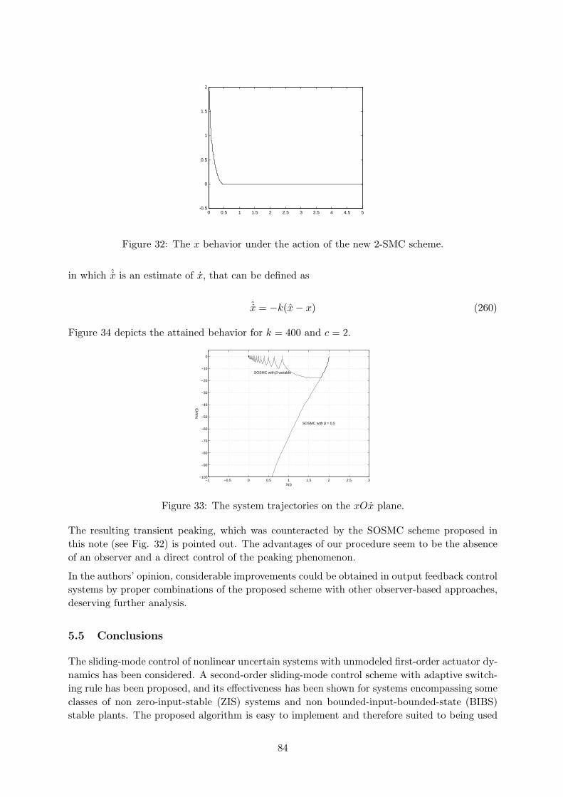
Theorem 1. Consider system (176), which verifies assumptions (181)–(182) and with xn notavailable. Let the sliding quantity s(t) be defined as in (177). Then, the digital control strategy(184)–(188) guarantees that, after a finite transient TR, the following conditions are satisfied atany t ≥ TR

|s(t)| ≤ O(T 2)|s(t)| ≤ O(T )

(189)

Proof. See the Appendix.

A similar result was attained by Drakunov et al. for systems with q = 1 and known controlgain [Drakunov et al. ‘2000], and then generalized to systems with unknown control gain in[Young et al. ‘99] and [Drakunov et al. ‘2000]. The use of a predictor of the uncertain dynamics

62

was the main point of the above approach, increasing by one the order of the accuracy providedby first order sliding mode control and reducing the control effort.

The aim of the present Chapter is that of showing that the application of second order slidingmode control strategies allows to achieve a system motion confined within a O(T 3) boundarylayer of the sliding manifold, that is the same accuracy featured by real third order sliding modecontrol. Note that, in any case, the attained motion cannot be defined as a third order slidingmode, since s has discontinuous dynamics [Levant ‘93].

In next section we derive a sufficiently accurate discrete model of the controlled plant which willbe used for the synthesis of two control strategies providing the desired accuracy.

4.4 A discrete time uncertain model with O(T 3) accuracy

Our first purpose is to provide a discrete model of the continuous system (179) with an approxi-mation, at any time instant, not worse than the accuracy of the sliding motion that it is wantedto be assured by the proposed digital control, that is O(T 3). To this end, let us indicate witha[k] = a(kT ) the k–th sample of a generic variable a. Assume that the control is applied bymeans of a ZOH.

Consider system (179), (181)-(182), and assume that the uncertainties are globally Lipschitz,i.e.

|ϕ[x(t)]| ≤ Φd (190)

|g[x(t)]| ≤ Γd (191)

Two subsequent samples of the sliding variable s satisfy the following relationship

s[k + 1] = s[k] +

∫ (k+1)T

kTs(τ)dτ (192)

The argument of the integral function, s(τ), can be reduced in Taylor series as follows:

s(τ) = s[k] + ϕ[k](τ − kT ) + g[k]u[k](τ − kT )+

+12

(

ϕ[x(ξ), x(ξ), ξ] + 12 g[x(ξ), ξ]u[k]

)

(τ − kT )2

τ ∈ [kT ; (k + 1)T ]ξ ∈ (kT ; (k + 1)T )

(193)

Considering (193) into (192) yields

s[k + 1] = s[k] + s[k]T +1

2[ϕ[k] + g[k]u[k]] T 2 + η1(T ) (194)

where η1(T ) is the discretization error due to the Taylor approximation in (193), satisfying, inaccordance with (190)-(191), the following constraint

|η1(T )| ≤ 1

6(Φd + Γdu[k])T

3 (195)

63

In order to obtain a discrete model effective for the synthesis procedure, the unavailable samples[k] in (194) must be eliminated. To this end, consider (194) in two subsequent sampling andsubtract one each other, then it follows

s[k + 1] = 2s[k] − s[k − 1] + (s[k] − s[k − 1])T++1

2 (ϕ[k] − ϕ[k − 1] + g[k]u[k] − g[k − 1]u[k − 1]) T 2 + η2(T )(196)

being, by (190)-(191),

|η2(T )| ≤[

1

3Φd +

1

6Γd(u[k] + u[k − 1])

]

T 3 (197)

By (193) it results

s[k] − s[k − 1] = ϕ[k − 1]T + g[k − 1]u[k − 1]T++1

2 (ϕ[x(ξ′), x(ξ′), ξ′] + g[x(ξ′), ξ′]u[k − 1])T 2

ξ′ ∈ ((k − 1)T ; kT )

(198)

and, consequently,

s[k] − s[k − 1] = (ϕ[k − 1] + g[k − 1]u[k − 1])T + η3(T ) (199)

with, by (190)-(191)

|η3(T )| ≤ 1

2(Φd + Γdu[k − 1]) T 2 (200)

Taking into account (196) and (199), the discrete time model of the sliding variable dynamics is

s[k + 1] = 2s[k] − s[k − 1] + ϕ[k − 1]T 2

+12 (g[k]u[k] + g[k − 1]u[k − 1])T 2 + ε[k]

k = 0, 1, 2 . . .(201)

At any sampling time, by (197) and (200), the discretization error ε[k] is such that

|ε[k]| ≤(

4

3Φd +

1

6Γdu[k] +

2

3Γdu[k − 1]

)

T 3 (202)

The discrete time sliding mode control problem can be therefore re–defined as that of finding,by means of the above approximate model, a control sequence u[k] (k = 0, 1, . . .) such that thesliding variable s is constrained within a O(T 3) boundary layer of the origin from a finite timeinstant on.

4.5 Discrete-Time Equivalent Control Based 2-SMC

The discrete model (201)-(202) may be used to define a digital control law ensuring that system(179), (181)-(182), (190)-(191) is confined within a small vicinity of the sliding set (30).

In [Utkin and Drakunov ‘93] the discrete–time equivalent control has been defined as the controlsequence u[k] such that s[k + 1] = 0 (k = 1, 2, . . .). The discrete equivalent control ud

eq[k]

64

(k = 1, 2, . . .) is able to drive the system into the sliding surface in one sampling period, and toconstrain on the system state in all the subsequent sampling time instants.

65

For the actual model, the discrete time equivalent control can be defined as

udeq[k] = − 1

gn[k]

(

gn[k − 1]u[k − 1] + d[k] + 22s[k]−s[k−1]T 2

)

(203)

where

d[k] = 2[

ϕ[k − 1] + 12 (∆g[k]u[k] + ∆g[k − 1]u[k − 1])

]

(204)

While it is conceptually very simple, the main problem in using the DTEC method is that theamplitude of the DTEC is inversely proportional to the sampling period T , unless some smallneighbor of the sliding manifold is reached. The size of this boundary layer is O(T ) as far assystems with relative degree one are dealt with [Drakunov et al. ‘93, Young et al. ‘99], whilecontracts to O(T 2) in the considered case [Bartolini et al. ‘99b]. In both cases, an initializationprocedure must be implemented in order to reach the admissible boundary layer in which theboundedness of the control signal is ensured.

In the case under investigation, the admissible O(T 2)-vicinity of the sliding manifold can bereached by means of the discrete-time 2-SMC scheme presented in the previous section. Fromthis point on the sliding variable can be steered to O(T 3) by means of the DTEC.

Unfortunately, the equivalent control is not directly measurable, due to the uncertain dynamicsof the controlled system, and some form of prediction must be implemented to estimate it.

The one-step-delay estimate of the uncertain term d[k] can be performed on the basis of theabove discrete model, delaying it by one sampling period, leading to

d[k] = s[k]−2s[k−1]+s[k−2]T 2 − 1

2 (gn[k − 1]u[k − 1] + gn[k − 2]u[k − 2]) (205)

If one put d[k] in place of d[k] in (203), and define udeq[k] accordingly, it yields

udeq[k] = 1

gn[k]

(

gn[k − 2]u[k − 2] − 23s[k]−3s[k−1]+s[k−2]T 2

)

(206)

After the initialization phase, the control udeq[k], which is available at the beginning of any control

interval, is used, and its effect on the reduction of the size of the boundary layer is stated inthe following Theorem. The stability of the sliding motion is nontrivial to demonstrate, andsuitable assumptions regarding the uncertainties are needed to ensure that the system trajectoryreaches, and does not leave, the O(T 3) boundary layer of s = 0.

Theorem 2: Consider system (176),(177) with its uncertain dynamics satisfying (181), (182),(190)-(191). Then the digital feedback controller

u[k] =

u1[k] if kT < TR

udeq[k] if kT ≥ TR

(207)

where u1[k] is the control strategy in Theorem 1, TR is the finite reaching time of a O(T 2)boundary layer and ud

eq[k] is defined as in (206), guarantees the finite-time reaching of a O(T 3)vicinity of the sliding manifold s = 0 characterized by

|s(t)| ≤ O(T 3)|s(t)| ≤ O(T 2)

(208)

66

Proof:

Once the O(T 2) boundary layer of s = 0 is reached in a finite time TR (Theorem 1) the controlcommutes from the discrete-time 2-SMC to the estimated DTEC (206). We must prove that,as a result, the boundary layer size contracts to O(T 3), and that the corresponding motion isstable.

To prove the assert, we start from the fact that, at any sampling time, the discretization errorintroduced by the discrete model (201) is O(T 3) [Bartolini et al. ‘99a].

It is not difficult to show that the behaviour of s[k] under the action of the proposed controlleris described by

s[k + 1] =1

2(d[k] − d[k − 1]) +O(T 3) (209)

which can be rewritten, by virtue of the smoothness assumptions (190)-(191), in the form

s[k + 1] =1

4∆g[k] (u[k] − u[k − 2]) +O(T 3) (210)

The coupling between s[k] and u[k] makes necessary the analysis of the closed loop behaviour ofthe system in a neighbor of the sliding manifold.

By the above considerations, as the control effort does not depend on the sampling time T ,substituting the expression for the DTEC into (210), it results

s[k + 1] = 12

∆g[k]gn[k] (3s[k] − 3s[k − 1] + s[k − 2]) +O(T 3) (211)

i.e, a third order difference equation. Considering the frozen discrete models obtained for allpossible values of ∆g[k] and gn[k], the discrete system (211) has all poles inside the unit circlefor sufficiently small ∆g[k]. The admissible uncertainties in the control gain are dictated bythe above stability condition, together with the ”small” variation of ∆g[k]/gn[k] (i.e., Gd issufficiently small) that ensures that the stability of the whole set of the above frozen modelsimplies the stability of the overall time varying discrete system. It is easy to derive conditions(208) from the analysis of (211), which is a stable difference equation with a O(T 3) disturbingterm.

4.6 Simulation results

Consider system (176), with n = 3 and

f(x, t) = 3 + sin(10t+ x1) ∗ cos(x22 + x2

3)g(x, t) = 1 + 0.5sin(3 + x1 + x2)

(212)

x3 is not available for measurements, and the initial conditions are set to x(0) = [1, 1, 1]. Thecontrol task is to reduce the state vector components to zero, and the sliding manifold is s =x2 + 2x1 = 0 is defined. A sampling period of T = 10−4s is used.

The nominal control gain on the basis of which it is computed the control law is

gn(x) = 2 + sin(3 + x1 + x2) (213)

67

i.e. the actual control gain parameters are assumed to differ by the 50% with respect to thenominal ones.

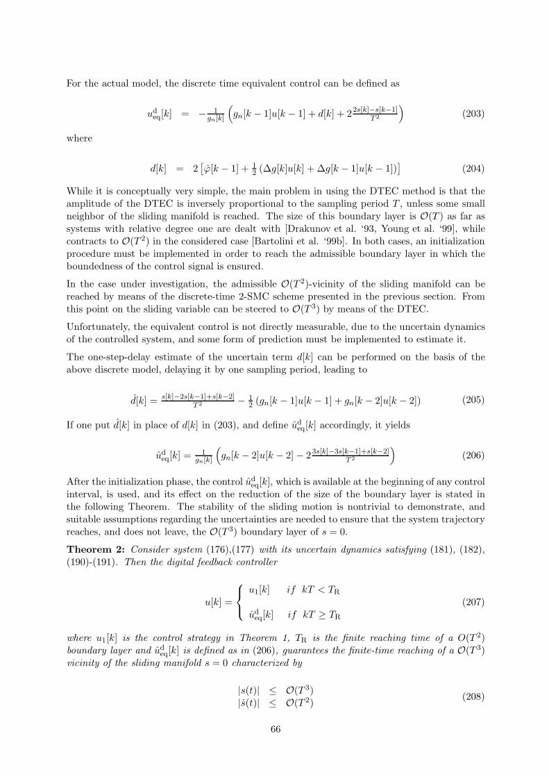
The control strategy in Theorem 2 is implemented with α∗ = 1, UM = 20 and TR = 2s. Themodification of the controller at t = TR is apparent from Fig. 24.

0 1 2 3 4

-20

-10

0

10

20

Actu

al c

ontro

l

Time [sec]

Figure 24: The actual control.

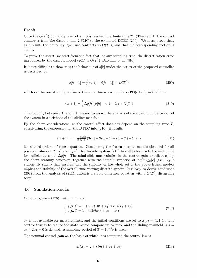
In the steady state, the actual control turns out to track the equivalent control, as it is evidencedin Fig. 25.

2 3 4-10

0

10

ue q (t)u(t)

The

actu

al a

nd e

quiv

alen

t con

trol

Time [sec]

Figure 25: The actual control and the equivalent control.

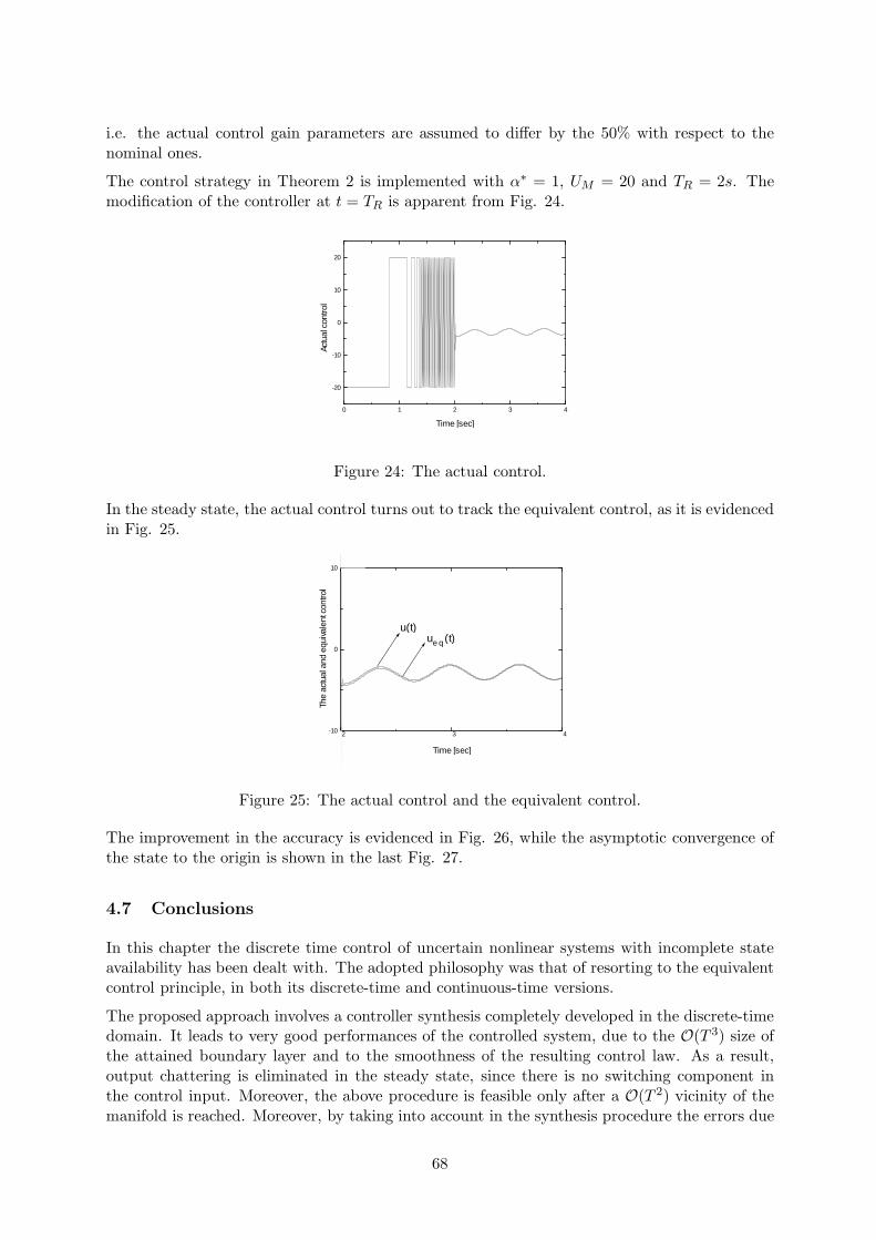
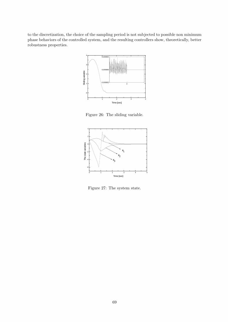
The improvement in the accuracy is evidenced in Fig. 26, while the asymptotic convergence ofthe state to the origin is shown in the last Fig. 27.

4.7 Conclusions

In this chapter the discrete time control of uncertain nonlinear systems with incomplete stateavailability has been dealt with. The adopted philosophy was that of resorting to the equivalentcontrol principle, in both its discrete-time and continuous-time versions.

The proposed approach involves a controller synthesis completely developed in the discrete-timedomain. It leads to very good performances of the controlled system, due to the O(T 3) size ofthe attained boundary layer and to the smoothness of the resulting control law. As a result,output chattering is eliminated in the steady state, since there is no switching component inthe control input. Moreover, the above procedure is feasible only after a O(T 2) vicinity of themanifold is reached. Moreover, by taking into account in the synthesis procedure the errors due

68

to the discretization, the choice of the sampling period is not subjected to possible non minimumphase behaviors of the controlled system, and the resulting controllers show, theoretically, betterrobustness properties.

0 1 2 3 4

0

1

2

3

4

Slid

ing

varia

ble

Time [sec]

2-0,000002

0,000000

0,000002

Figure 26: The sliding variable.

0 1 2 3 4 5

-6

-4

-2

0

2

4

x3

x2

x1

The

stat

e va

riabl

es

Time [sec]

Figure 27: The system state.

69

APPENDIX

Proof. of Theorem 1

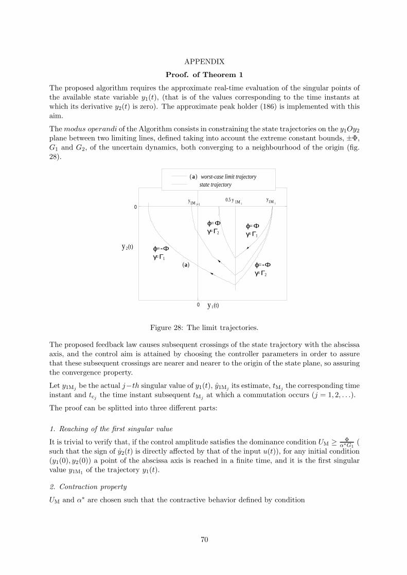
The proposed algorithm requires the approximate real-time evaluation of the singular points ofthe available state variable y1(t), (that is of the values corresponding to the time instants atwhich its derivative y2(t) is zero). The approximate peak holder (186) is implemented with thisaim.

Themodus operandi of the Algorithm consists in constraining the state trajectories on the y1Oy2

plane between two limiting lines, defined taking into account the extreme constant bounds, ±Φ,G1 and G2, of the uncertain dynamics, both converging to a neighbourhood of the origin (fig.28).

ϕ=-Φγ=Γ1

(a)

ϕ=Φγ=Γ2

ϕ=-Φγ=Γ2

ϕ=Φγ=Γ1

y 1(t)

y 2(t)

0

0y1M i+1

0.5 y1M iy1M i

(a ) worst-case limit trajectory state trajectory

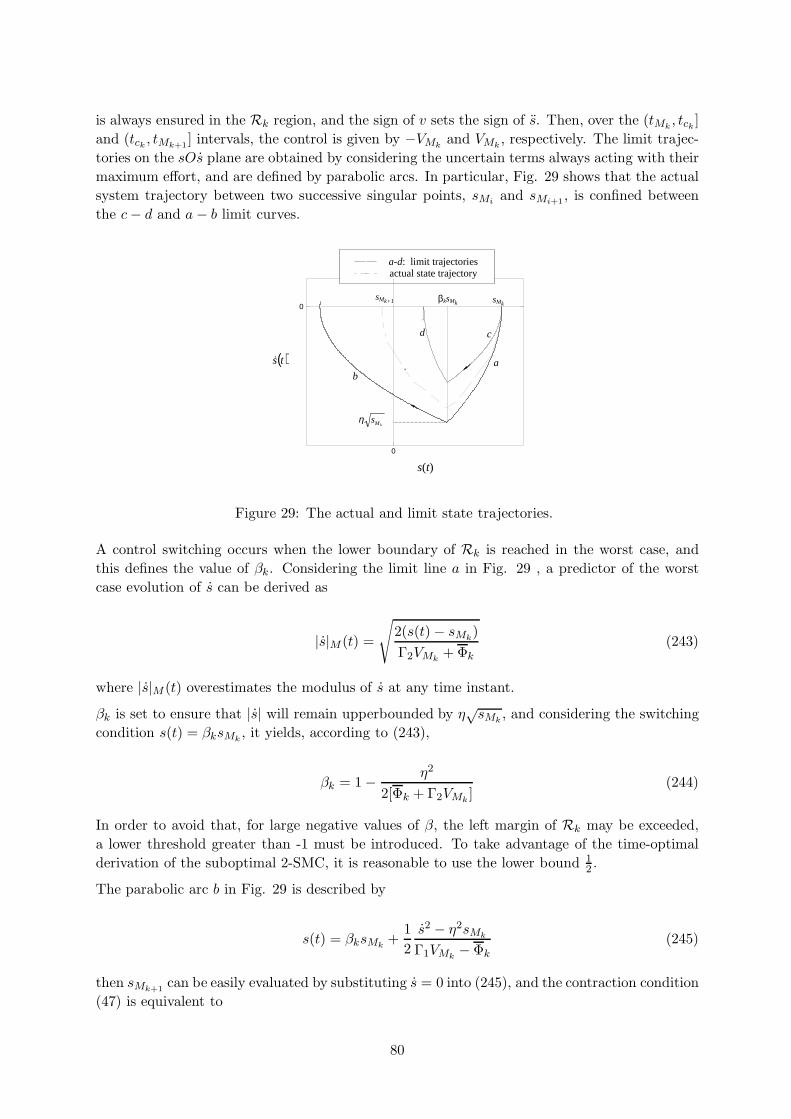
Figure 28: The limit trajectories.

The proposed feedback law causes subsequent crossings of the state trajectory with the abscissaaxis, and the control aim is attained by choosing the controller parameters in order to assurethat these subsequent crossings are nearer and nearer to the origin of the state plane, so assuringthe convergence property.

Let y1Mjbe the actual j−th singular value of y1(t), y1Mj

its estimate, tMjthe corresponding time

instant and tcjthe time instant subsequent tMj

at which a commutation occurs (j = 1, 2, . . .).

The proof can be splitted into three different parts:

1. Reaching of the first singular value

It is trivial to verify that, if the control amplitude satisfies the dominance condition UM ≥ Φα∗G1

(such that the sign of y2(t) is directly affected by that of the input u(t)), for any initial condition(y1(0), y2(0)) a point of the abscissa axis is reached in a finite time, and it is the first singularvalue y1M1

of the trajectory y1(t).

2. Contraction property

UM and α∗ are chosen such that the contractive behavior defined by condition

70

|y1Mj+1| < |y1Mj

| j = 1, 2, . . . (214)

takes place.

Suppose, without loss of generality, that the actual value of the j− th singular value is such thaty1Mj

> 0 , i.e. it lies on the right side of the abscissa axis. Due to the symmetry of the problemwith respect to the origin of the state plane, analogous consideration are also valid if y1Mj

< 0 .

Due to the sampled nature of the measures, the updating of the gain coefficient α[k] and theswitching of the control can occur with a delay at most equal to T with respect to the ideal onesin t = tMj

and in y1[k] = 12 y1M[k] respectively.

Consequently, at the actual switching time instant t = tcj, the states satisfy the following

conditions

y1(tcj) ∈ [12y1Mj

− 116(Φ +G2UM)T 2 − 1

2(Φ + α∗G2UM)T 2

−T√

y1Mj(Φ + α∗G2UM) + aT 2 , 1

2y1Mj]

y2(tcj) ∈ [−(Φ + α∗G2UM)T −

√

y1Mj(Φ + α∗G2UM) + aT 2 ,

−√

y1Mj(Φ − α∗G1UM)]

(215)

a =1

8(Φ +G2UM)[(Φ + α∗G2UM) + 18G2UM(1 − α∗)] (216)

As the system trajectory is constrained between the limit lines in fig. 28, the subsequent crossingof the abscissa axis belongs to the interval

y1Mj+1∈ [−1

2(α∗G2−G1)UM+2Φ

G1UM−Φ y1Mj− bT 2

−G1+α∗G2

G1UM−ΦUMT√

y1Mj(Φ + α∗G2UM) + aT 2 ,

12

(G2−α∗G1)UM+2ΦG2UM+Φ y1Mj

]

(217)

b = 116 (Φ +G2UM)

[

(G1+α∗G2)G1UM−Φ UM

]

+ 98(Φ +G2UM)(1 − α∗)G2UM+

+12(Φ + α∗G2UM)

[

(G1+α∗G2)G1UM−Φ UM

] (218)

Define the following normalized non negative variables

z =UM

Φ(219)

ρ =|y1Mj

|ΦT 2

(220)

Sufficient condition for the fulfillment of the contraction condition (214) is represented by thefollowing system of inequalities

ρ ≥ 0z ≥ 1

α∗G1

(3G1 − α∗G2)z − 4 > (G1 + α∗G2)(1 + α∗G2z)zρ+

+18 [G1 + (18 − 17α∗)G2](1 +G2z)

zρ+

+2(G1 + α∗G2)zρ

√

(1 + α∗G2z)ρ+ 18(1 +G2z)[1 + (18 − 17α∗)G2z]

(221)

71

The second inequality represents the control’s dominance condition, ensuring that the sign ofthe control u(t) sets the sign of y2(t) . The third inequality in (221) defines the set Z ⊆ Rsuch that, ∀z ∈ Z, the points of the straight line defined by the left-hand side term w1(z) =(3G1 − α∗G2)z − 4 lie above the points of the parametric function

w2(z) = (G1 + α∗G2)(1 + α∗G2z)zρ + 1

8 [G1 + (18 − 17α∗)G2](1 +G2z)zρ+

+2(G1 + α∗G2)zρ

√

(1 + α∗G2z)ρ+ 18(1 +G2z)[1 + (18 − 17α∗)G2z]

(222)

The function w2(z; ρ) crosses the origin of the cartesian plane zOw2, and it has a negativelocal minimum for z < 0 and positive first and second derivatives with respect to z if z > 0.Moreover, the value of the local minimum is an increasing function of the parameter ρ, andthe parametric function w2(z; ρ) degenerates into the abscissa axis as the parameter ρ goes toinfinity. By means of the above considerations it is possible to claim that the two lines definedby the functions w1(z) and w2(z; ρ) have at most two cross points, which degenerate into adouble contact point for a specific lower value of the parameter ρ called ρ∗. For values of ρ < ρ∗

there is no intersection between the two lines and system (221) has not solutions.

This fact imply that the convergence of the sliding variable and of its time derivative to zero isassured only if the the control amplitude is chosen within a proper open set.

The limits of the admissible set depend on ρ, nevertheless the control amplitude could be chosensuch that the non negative normalized variable ρ, defining the size of the boundary layer, canreach its minimum at ρ∗. In this case, the admissible set collapses into a single point, whichrepresent a sort of optimal value of the control amplitude, which minimizes the theoretical sizeof the corresponding boundary layer.

The ρ∗ value, and the corresponding point z = z∗, have been calculated in [Bartolini et al. ‘98c]under the assumption that no gain affects the control input, that is G1 = G2 = α∗ = 1, leadingto the following approximate solution

ρ∗ = 85z∗ = 6

(223)

This means that, if G1 = G2 = α∗ = 1, then UM = 6F is the control effort that minimizes thesize of the boundary layer.

By re–considering the general case, it can be noted that, as ρ∗ does not depend on T , then, by(215), (216) and (220),Theorem’s statement (189) is directly derived.

The dependence of the bounds of the admissible set Z by the sampling period T can be inves-tigated by analyzing the limit behaviour of system (221) for T → 0.

Since ρ = O(T−2), an intersection between w1(z, ρ) and w2(z) can occur iff z = 43G1−α∗G2

+O(T )

or z = O(T−2).

By these considerations, (185) is directly justified. So the Theorem is proved.

3. Finite time reaching of the boundary layer

As the time interval between two subsequent singular values of y1(t) is finite, the finite timeconvergence of the system to the residual set is a straightforward consequence of the contractioncondition.

72

References

[Bartolini et al. ‘95] G. Bartolini, A. Ferrara, V.I. Utkin, “Adaptive sliding mode control indiscrete time systems”, Automatica, vol. 31, no. 6, pp. 769–773, 1995

[Bartolini et al. ‘97] G. Bartolini, A. Ferrara, E. Usai, “Output Tracking Control of UncertainNonlinear Second-Order Systems”, Automatica, vol. 33, no. 12, pp. 2203–2212, 1997

[Bartolini et al. ‘98a] G. Bartolini, A. Ferrara and E. Usai, “Chattering Avoidance by SecondOrder Sliding Mode Control”, IEEE Trans. on Aut. Control, 43, 241–246 (1998)..

[Bartolini et al. ‘98b] G. Bartolini, A. Ferrara, A. Pisano, E. Usai, “Adaptive reduction of thecontrol effort in chattering free sliding mode control of uncertain nonlinear systems”, App.Math. and Computer Science, vol. 8, no. 1, pp. 51–71, 1998

[Bartolini et al. ‘98c] G. Bartolini, A. Pisano, E. Usai, “Digital Second Order Sliding Mode Con-trol of SISO Uncertain Nonlinear Systems”, Proc. of the 1998 American Control ConferenceACC’98, vol. 1, pp. 119–124, Philadelfia, Pensylvania, June 1998

[Bartolini et al. ‘99a] G. Bartolini, A. Ferrara, A. Levant, E. Usai “On Second Order Slid-ing Mode Controllers”, in “Variable Structure Systems, Sliding Mode and Nonlinear Con-trol”, K.D. Young and U. Ozguner eds., Lecture Notes in Control and Information Sciences,Springer-Verlag, 247, 329-350, (1999).

[Bartolini et al. ‘99b] G. Bartolini, A. Pisano, E. Usai “Variable Structure Control of NonlinearSampled Data Systems by Second Order Sliding Modes”, in “ Variable Structure Systems,Sliding Mode and Nonlinear Control”, K.D. Young and U. Ozguner eds., Lecture Notes inControl and Information Sciences, Springer-Verlag, vol. 247, 43-68, (1999).

[Drakuno and Utkin ‘90] S.V. Drakunov, V.I. Utkin, “Sliding mode in dynamic systems”, Int.Journal of Control, vol. 55, pp. 1029–1037, 1990

[Drakunov et al. ‘93] S.V. Drakunov, U. Ozguner, W.C. Su, K.D. Young, “Sliding Mode withChattering Reduction in Sampled Data Systems”, Proc. of the 32th Conf. on Decision andControl - CDC’93, pp. 2452–2457,

[Drakunovet al. ‘96] S.V. Drakunov, U. Ozguner, W.C. Su, “Implementation of Variable Struc-ture Control for Sampled–Data Systems”, in Robust Control via variable structure and Lya-punov techniques. F.Garofalo and L.Glielmo eds., Lecture Notes in Control and InformationScience no. 217, pp. 87–106, Springer-Verlag, London, 1996

[Drakunov et al. ‘2000] S.V. Drakunov, U. Ozguner, W.C. Su “An O(T 2) Boundary Layer inSliding Modefor Sampled Data Systems”, IEEE Trans. on Aut. Control, 45, 482–485 (2000)..

[Furuta ‘90] K. Furuta, “Sliding mode control of a discrete system”, System and Control Letters,vol. 14, no. 2, pp. 145–152, 1990

[Furuta and Pan ‘94] K. Furuta, Y. Pan, “VSS controller design for discrete time systems”,Control Theory and Advanced Technology, vol. 10, no. 4/1, pp. 669–687, 1994

[Levant ‘93] A. Levant, “Sliding order and sliding accuracy in sliding mode control”, Int. Journalof Control, vol. 58, pp. 1247–1263, 1993.

73

[Milosavljevic ‘85] C. Milosavljevic, “General conditions for the existence of a quasisliding modeon the switching hyperplane in discrete variable systems”, Automation Remote Control, vol.43, no. 1, pp. 307–314, 1985

[Young et al. ‘99] D. Young, U. Ozguner and V. Utkin “A control engineers guide to slidingmode control”, IEEE T-CST, vol. 7, pp. 328–342, 1999.

[Utkin and Drakunov ‘93] V.I. Utkin, S.V. Drakunov, “On Discrete–Time Sliding Mode Con-trol”, Proc. of the IFAC Symposium on Nonlinear Control Systems - NOLCOS, pp. 484–489,Capri, Italy, 1989, San Antonio, Texas, December 1993

[Utkin ‘93] V.I. Utkin, “Sliding Mode Control in Discrete–Time and Difference Systems”, inVariable Structure and Lyapunov Control. A.S.I. Zinober ed., pp. 83–102, Springer-Verlag,London, 1993

74

5 2-SMC with global convergence properties

5.1 Preliminaries

All the results presented in previous chapters were based on some assumptions regarding the

existence of suitable upperbounds to the drift term and control gain of the second-order sliding

dynamics. In particular, it has to be pointed out that all 2-SMC schemes up to now published in

the literature are based on the standing assumption that the drift term has a linear growth with

respect to the sliding variable derivative. In many cases, especially when a nonlinear dynamic

actuator is present at the input of the plant, this assumption prevents the effectiveness of 2-SMC

strategies.

In this chapter it is proposed a new algorithm that overcomes such limitations by means of an

adaptive switching rule

The affine dependence on the control was a further important standing assumptions of previous

treatments, and it will be relaxed at the same time in this chapter.

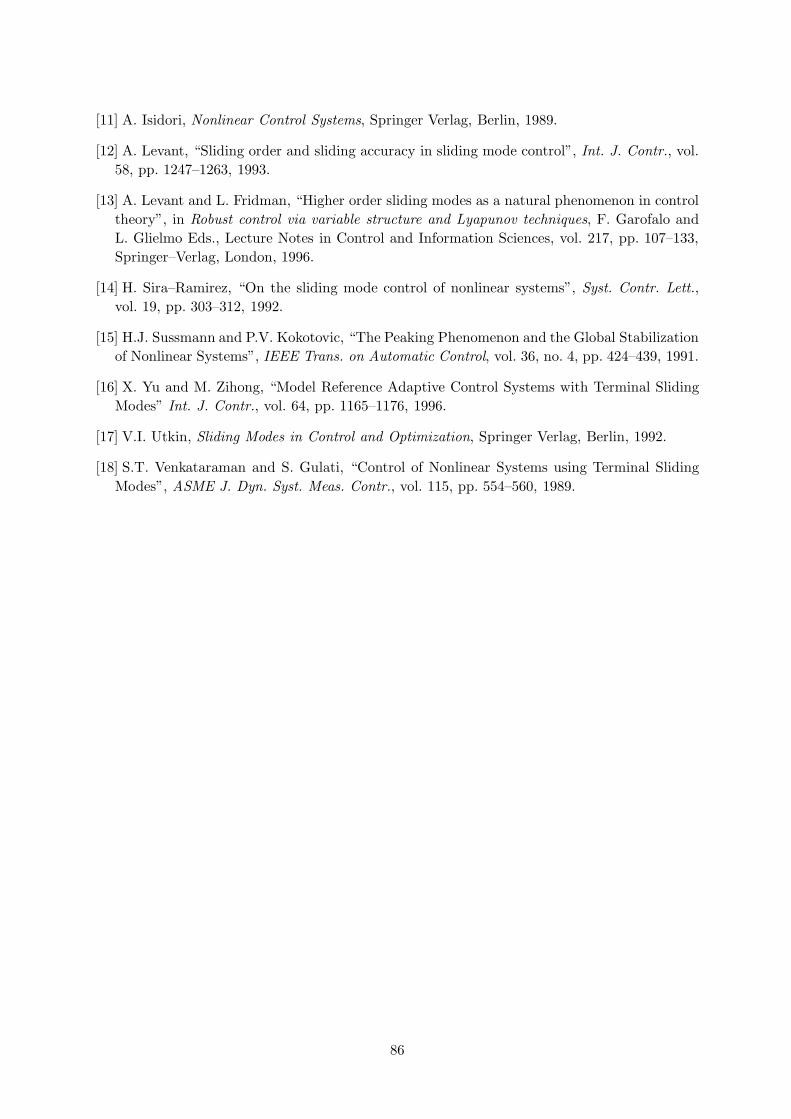
It will be also shown that the proposed algorithm is able to have a direct control on the peaking

behaviour that often affects the transient of nonlinear uncertain systems. So, the proposed

approach reveals to be an effective alternative to the use of saturating filters at the inputs.

5.2 Problem Formulation

Consider a nonlinear single–input system that can be modeled by a differential equation in

normal form with non-affine dependence on the control input, that is,

x(n) = f(x, u) (224)

and assume that the actuator has a first-order dynamics of the type

u = h(u) + v (225)

where x = [x, x, . . . , x(n−1)] ∈ Rn is the measurable state vector, u ∈ R is the plant input, v ∈ R

is the actuator input, and f(x, u), h(u) are sufficiently smooth uncertain functions. Let any

solutions of (224),(225) be well defined for all t > 0, provided that v is bounded and continuous.

The problem of generalizing the globality features of the 2-SMC approach to wider class of

systems, that can be obtained by combining existing techniques (backstepping and so on) with

2-SMC (see, for instance, [2]) is postponed to further works.

It is well known that if the system output is defined by a proper linear combination of the state

variables

s(x) = cx (226)

where c = [c1, c2, . . . cn−1, 1] and ci (i = 1, 2, . . . , n− 1) are real positive constants such that the

polynomial P (z) = zn−1 +∑n−1

i=1 cizi−1 is a Hurwitz one, then the origin of the state space is a

globally asymptotically stable (GAS) equilibrium point for the corresponding zero dynamics.

From (224)-(226), it follows

75

˙x(t) = Ax(t) + bs(t)xn(t) = −cx + s(t)

s(t) = f(x, u) +∑n−1

i=1 cixi+1 = k(x, u)s(t) = ϕ(x, u) + γ(x, u)v

(227)

where x = [x1, x2, . . . , xn−1]T , c = [c1, c2, . . . , cn−1], A is an (n−1)×(n−1)–matrix in companion

form with the last row coinciding with the vector −c, b = [0, . . . , 0, 1]T ∈ Rn−1, and

ϕ(x, u) =∑n−1

i=1∂f(x,u)

∂xi

xi+1 +(

∂f(x,u)∂xn

+ cn−1

)

f(x, u) +∑n−2

i=1 cixi+2 + ∂f(x,u)∂u

h(u)

γ(x, u) = ∂f(x,u)∂u

(228)

Assume that the map k(x, ·) is one to one on any subset u ∈ U ⊆ R. We refer the reader to [6],

and references therein, for a survey of many explicit sufficient conditions on the global injectivity

of ϕ(x, ·). Our attention is focused on smooth maps falling into the classes therein considered.

The unique solution (if any) u ∈ U of the equation

k(x, u) = w (229)

for any given w ∈ R, will be denoted by u∗(x, s).

On the basis of the above considerations, assume the following

|ϕ(x, u)| ≤ Φ [‖x(t)‖, |u|] ≤ Φ(‖x(t)‖, |u∗(x, s)|) ≤ Φ(‖x(t)‖, |s|) (230)

|h(u)| ≤ H(u) (231)

0 < Γ1 ≤ γ(x, u) ≤ Γ2 (232)

where Γ1, Γ2 are known positive constants and Φ(·), Φ(·), H(u) are known positive radially-

non-decreasing functions without any particular assumption about their growth.

According to the above assumptions and considerations, the stabilization problem for system

(224),(225) can be reduced to the finite-time stabilization of the second-order uncertain system

described by the last two equations in (227). As the uncertain system is of relative degree two,

a 2-SMC approach appears reasonable.

In previous chapter a class of systems with affine dependence on the control was considered. In

that case, if the actual control u were directly modifiable, the relay control the control would

act directly on s).

If a first-order unmodeled actuator dynamics of the type

u(t) = h(u) + v(t) (233)

is taken into account, where v(t) is the actuator input and h(u) is unknown, the relative degree

is under-estimated, so the above procedure might fail.

By singular perturbation analysis, it has been proven that 1-SMC is robust to the sufficiently

fast unmodeled dynamics of the actuators [17]. A discontinuous control v(t) can lead to either a

76

stable or an unstable second-order sliding mode (i.e., a sliding motion on the manifold s = s = 0),

depending on the actual actuator dynamics [13].

Here the presence of the actuator dynamics is considered explicitly, and a suitable control strat-

egy is developed.

It is worth noting that a control

v(t) = −(Φ(‖x‖, |u|) + k2)sign(s(t) − s(t0)) (234)

globally forces s in a finite time tM1to zero, t0 being the initial control time. Therefore, the

starting point of the proposed procedure can be regarded as a singular point of the s variable,

s(tM1), tM1

s.t. s(tM1) = 0.

At t = tM1, it would be necessary to evaluate constant upper bounds to the uncertainties. As

a result, the control strategy in chapter 3 could be applied, but the following problem would

arise: how can one choose the control effort at the time instant tM1such that, at least until

the subsequent singular point is reached, the uncertain drift term |ϕ(x, u)| increases without

exceeding the constant bound on the basis of which the control amplitude has been evaluated?

The sign and modulus of v remain constant until a commutation condition of the type s(tc1) =

βsM1(β = 0 for the twisting algorithm, β = 1

2 for the suboptimal algorithm) is encountered,

and then the sign of v changes. If, before this event occurs, the uncertainty exceeds the constant

limit on the basis of which the control amplitude VM has been computed, the method might

fail, in that the existence of both the commutation instant and the subsequent singular point

cannot be guaranteed.

With a constant β, the solutions to the problems of predicting a constant upper bound to |ϕ(·)|and of choosing, accordingly, the controller parameters VM and α such that, over the entire

control time interval, the uncertainty does not exceed the predicted upperbound exist only for

systems with an affine dependence of the drift term ϕ(x, u, t) on the plant control u [4].

When this assumption is not verified, the controller structure has to be modified. The solution

proposed in this paper, called “solution with variable β”, exploits the idea of selecting the

commutation instants on line, as soon as a current overestimate of the uncertain drift term

modulus is equal to a pre-specified value. After the commutation, it can be proved that a new

singular point, closer to the origin than the previous one, is reached at t = tM2, whereas the

uncertainties are kept below the pre-specified threshold. The repetition of the same procedure

over any successive interval[

tMi, tMi+1

]

(i = 2, 3, . . .) ensures that the convergence to the sliding

manifold will take place in a finite time.

In the next section this approach is described and its global convergence properties are proven.

Section 3 deals with simulation results, and, in Section 4, some final conclusions are drawn.

5.3 Main result

Our proposed approach can be summarized as follows.

First, we define a compact region R in the state space containing the 2-sliding set s = s = 0;

within this region, constant bounds to the uncertainties can be found. Then, the control must

be able to accomplish the following tasks:

1. globally driving the system trajectories into the region R in a finite time;

77

2. constraining the system motion within this region over the entire control time interval;

3. guaranteeing the finite-time reaching of the 2-sliding manifold s = s = 0

To this end, consider the rectangular region on the sOs plane

Rk ≡

(s, s) ∈ R2 : |s| ≤ |sMk|, |s| ≤ η

√

|sMk|

(235)

where sMkis the generic k–th singular value of s, (sMk

= s(tMk), tMk

: s(tMk) = 0), and η is a

positive design parameter to be specified on the basis of the control requirements. In the region

Rk, a constant upper bound to the uncertain drift term modulus |ϕ(x, u)| is given by (230) as

Φk = Φ

(

‖xMk‖, η√

|sMk|)

(236)

where ‖xMk‖ is an upper bound to ‖x‖, whenever the output phase trajectory is within the

region Rk. Due to the bounded-input-bounded-state (BIBS) property of the linear subsystem

in (227), the following relationship holds [4]

‖x(t)‖ ≤ ‖xMk‖ = Qx‖x(tMk

)‖ +Qy|sMk| t ≥ tMk

(237)

where Qx and Qy are properly defined constants.

The control strategy is designed such that the controlled plant may reach, and then never leave,

any region Rk.

During the initialization phase, the system is globally driven in a finite time toward the s = 0

axis, that is, a first singular point sM1is attained after a finite transient process. Then the

control signal v is defined such that a sequence of singular values sMk= s(tMk

), k = 2, 3, . . .,

satisfying the contraction condition (47) is generated. This implies that Rk+1 ⊂ Rk and that

Rk → O in a finite time, O being the origin of the sOs plane.

The possibility of accomplishing this twofold task strictly depends on the assumptions made on

the uncertain plant dynamics. In previous works, the problem has been solved by assuming that

the the modulus of the uncertain drift term ϕ(x, u) in (228) increases linearly with the control

magnitude |u| [3, 4]. This assumption ensures that the inequality representing the algebraic

loop between the control amplitude and the uncertainty bounds (the amplitude depends on the

bounds and vice versa) will be solved. In case |ϕ(x, u)| were nonlinear with respect to |u|, a

solution could not exist.

In this note, it is shown that, if the anticipating factor β in the switching logic is properly

adjusted, two main results are obtained. First, the modulus of the output derivative can be

maintained smaller than a pre-specified value, thus counteracting the peaking phenomenon;

secondly, the controlled class of plants is enlarged, now encompassing a class of systems nonlinear

in the control law and/or with nonlinear dynamic actuators.

The control algorithm based on the above considerations is formally defined by the following

Theorem:

Theorem 1: Consider system (224)-(225) with a completely available state. Let the sliding

output s be defined according to (226), and let it be such that the corresponding zero-dynamics

78

is asymptotically stable. Assume that the uncertain input-output dynamics (227)-(228) satisfies

(230)-(232).

The control law

v(t) =

− 1Γ1

[Φ [‖x(0)‖, |u(0)|] + χ] sign (s(0)) t = 0

− 1Γ1

[Φ [‖x(t)‖, |u(t)|] + χ] sign (s(t) − s(0)) 0 < t ≤ tM1

χ > 0 (238)

ensures the reaching of a first singular point sM1at the time instant t = tM1

≤ ˙s(0)χ . From this

point on, the control law

v(t) = −VMksign [s(t) − βksMk

] tMk< t ≤ tMk+1

k = 1, 2, . . . (239)

guarantees the finite-time vanishing of the system output s and of its derivative, provided that

the controller parameters are chosen according to

VMk=

α

Γ1

[

Φk +1

3η2

]

α > 1 (240)

βk = max

1

2, 1 − η2

2[Φk + Γ2VMk]

(241)

where η is a positive constant, Φk is defined in (236),(237), tMkare the time instants at which

s is zero, and sMk= s(tMk

). As a consequence, the state x(t) globally exponentially converges

to zero.

Proof.

Initialization phase: 0 ≤ t ≤ tM1

The initialization phase is designed such that the axis s(t) = 0 is reached in a finite time tM1.

According to (238), and taking into account (230)-(232), the sign of s is forced to be opposite to

that of s. The behavior of the system is different in the two cases s(0)s(0) > 0 and s(0)s(0) < 0.

In the former case, |s| monotonically converges to zero with no switchings of the control sign.

In the latter case, the same behavior is attained with an instantaneous switching of the control

at t = 0+. In both cases, at t = tM1< (s(0)/χ), a first singular value of s(t), sM1

, is reached,

and this value is available for control purposes.

Reaching phase tMk< t ≤ tMk+1

(k = 1, 2, . . .)

Let sMkbe the k–th singular value of s(t), tMk

the corresponding time instant, and tckthe time

instant (following tMk) at which a control switching occurs.

Suppose, without loss of generality, that sMkis positive. Due to the symmetry of the limit

trajectories, analogous considerations still apply in the case sMk< 0 .

The proof of the finite-time convergence to the origin of the state plane can be split into the

following steps.

Contraction property:

According to (240), the control magnitude is such that the dominance condition

Γ1VMk> Φk (242)

79

is always ensured in the Rk region, and the sign of v sets the sign of s. Then, over the (tMk, tck

]

and (tck, tMk+1

] intervals, the control is given by −VMkand VMk

, respectively. The limit trajec-

tories on the sOs plane are obtained by considering the uncertain terms always acting with their

maximum effort, and are defined by parabolic arcs. In particular, Fig. 29 shows that the actual

system trajectory between two successive singular points, sMiand sMi+1

, is confined between

the c− d and a− b limit curves.

0

0

ba

a-d: limit trajectories actual state trajectory

( )ts

s(t)

sMksMk+1

kMsη

cd

βksMk

Figure 29: The actual and limit state trajectories.

A control switching occurs when the lower boundary of Rk is reached in the worst case, and

this defines the value of βk. Considering the limit line a in Fig. 29 , a predictor of the worst

case evolution of s can be derived as

|s|M (t) =

√

2(s(t) − sMk)

Γ2VMk+ Φk

(243)

where |s|M (t) overestimates the modulus of s at any time instant.

βk is set to ensure that |s| will remain upperbounded by η√sMk

, and considering the switching

condition s(t) = βksMk, it yields, according to (243),

βk = 1 − η2

2[Φk + Γ2VMk]

(244)

In order to avoid that, for large negative values of β, the left margin of Rk may be exceeded,

a lower threshold greater than -1 must be introduced. To take advantage of the time-optimal

derivation of the suboptimal 2-SMC, it is reasonable to use the lower bound 12 .

The parabolic arc b in Fig. 29 is described by

s(t) = βksMk+

1

2

s2 − η2sMk

Γ1VMk− Φk

(245)

then sMk+1can be easily evaluated by substituting s = 0 into (245), and the contraction condition

(47) is equivalent to

80

0 <1

2

η2

Γ1VMk− Φk

< 1 + βk (246)

Taking into account that βk ∈ [12 , 1), condition (246) is satisfied, whatever βk may be, provided

that VMkis chosen according to (240); then the region Rk is never left during the considered

time interval t ∈ (tMk, tMk+1

].

If condition (246) is satisfied at any k, then a real positive constant ν2 < 1 such that |sMk+1| <

ν2|sMk| (k + 1, 2, . . .) can always be defined; therefore, if one sets

sMk= sup

t∈[tMk,tMk+1

]|s(t)| (247)

one obtains

|sMk+1| ≤ ν2k|sM1

|sMk

≤ ηνk−1√

sM1

(248)

which implies |sMk| → 0 and |sMk

| → 0 as k → ∞.

Finite time convergence:

Starting from (sMk, 0) at the time instant t = tMk

and considering the limit trajectories a − b

and c − d in Fig. 29 , it can be proved that the a − b trajectory is slower than the c − d one.

Algebraic computations lead to

tabMk+1

= tMk+√

2(1 − βk)

(Γ1 + Γ2)VMk+ 2Φk

(Γ2VMk+ Φk)

√

Γ1VMk− Φk

√

|sMk| (249)

Relying on the contraction property, the terms Φk and VMkare bounded; then it is possible to

define the constant

Ψ = maxk

√

2(1 − βk)

[

(Γ1 + Γ2)VMk+ 2Φ∗

k

(Γ2VMk+ Φ∗

k)√

Γ1VMk− Φ∗

k

]

(250)

and hence

tabMk+1

≤ tMk+ Ψ

√

|sMk| (251)

from which one recursively derives

tabMk+1

≤ tM1+ Ψ

k∑

j=1

√

|sMj| (252)

Taking into account (248), the finite-time convergence is proved as the following relationship

holds

81

Tr = limk→∞

tabMk+1

≤ tM1+ Ψ

√

|sM1|

1 − ν(253)

Remark: Because of the lack of information assumed in the statement of the problem, the

sufficient conditions stated in Theorem 1 are derived on the basis of a worst-case analysis, thus

they are very conservative. Computer simulations show that the control effort may be set to

smaller values than those in (240), thus one can obtain a higher smoothness of the resulting

control law and a higher accuracy in the practical realization of the control scheme; the control

effort may be set even to a-priori established constant values, thus one can reduce the on-line

computational effort.

5.4 Some simulation examples

In this section, the proposed procedure is illustrated and compared with other methodologies

by means of a simple, yet challenging, example.

Consider the dynamic system

x = ax2 + u |a| ≤ 4 (254)

with the actuator dynamics

τ u = −u+ v (255)

Assume that the control objective is to stabilize it in a finite time; then, x = 0 can be defined

as the sliding manifold, and the 1-SMC scheme

v = −(k2 + 4x2)sign(x) (256)

guarantees the global convergence of x to zero if τ = 0 (i.e. if u = v).

Transient peaking and instability occur for increasing values of τ (as pointed out in Fig. 30 ) if

one sets a = 2, k2 = 1.

0,0 0,5 1,0 1,5 2,0 2,5 3,0-2

-1

0

1

2

3

4

5

τ = 0.2

τ = 0

τ = 0.3

Time [sec]

Figure 30: 1-SMC. The x behaviour for different values of τ .

82

A sensible way to recover stability is to use sliding-mode control algorithms for systems of

relative degree two (2-SMC algorithms). Differentiating twice the sliding output locally leads

to a second-order sliding dynamics such that it is possible to use one of the 2-SMC algorithms

presented in chapter 3.

Fig. 31 shows the state evolution when the suboptimal 2-SMC algorithm is implemented; the

peaking effect is pointed out.

Moreover, it may happen that the uncertain drift term ϕ(x, u) in (227) does not satisfy the

boundedness conditions relevant to the linear growth with respect to u. As an example, consider

system (254), and assume that the actuator dynamics is represented by

u = −u2 + v (257)

Then the second-order sliding dynamics is given by

x = 2x3 + 2xu+ u2 + v = ϕ(x, u) + v (258)

In this case, the nonlinear growth of |ϕ(x, u)| is not affine any more in the variable u; as a

consequence the “conventional” suboptimal 2-SMC scheme cannot be applied.

If one considers system (254),(257), for x(0) = 2 and u(0) = −4, the performance of the new

control scheme, which has been presented and discussed in the previous section, is displayed

in Fig. 32 , showing the x evolution. If one introduce the time-varying anticipating factor to

improve the convergence properties, outlined in the Introduction, the stability of the system can

be recovered and the peaking phenomenon is avoided as well.

0 1 2 3

-1

0

1

2

Time [sec]

Figure 31: 2-SMC (suboptimal algorithm). The x behaviour for τ = 0.3.

In Fig. 33 , the trajectories of the system on the phase plane are compared in the cases of

suboptimal 2-SMC and 2-SMC with variable β, showing that the former solution fails to cope

with the fast nonlinear growth of the uncertain actuator dynamics (257).

As mentioned in the previous section, a different way to deal with relative-degree-two systems,

widely used in output-feedback control, is to implement an observer of the output derivative.

Due to the uncertainties it is reasonable to use high-gain observers (HGO) [1], and the 1-SMC

strategy could be applied by exploiting the new sliding output

s1 = ˆx+ cx c > 0 (259)

83

0 0.5 1 1.5 2 2.5 3 3.5 4 4.5 5-0.5

0

0.5

1

1.5

2

Figure 32: The x behavior under the action of the new 2-SMC scheme.

in which ˆx is an estimate of x, that can be defined as

ˆx = −k(x− x) (260)

Figure 34 depicts the attained behavior for k = 400 and c = 2.

−1 −0.5 0 0.5 1 1.5 2 2.5 3−100

−90

−80

−70

−60

−50

−40

−30

−20

−10

0

X(t)

Xdo

t(t)

SOSMC with β = 0.5

SOSMC with β variable

Figure 33: The system trajectories on the xOx plane.

The resulting transient peaking, which was counteracted by the SOSMC scheme proposed in

this note (see Fig. 32) is pointed out. The advantages of our procedure seem to be the absence

of an observer and a direct control of the peaking phenomenon.

In the authors’ opinion, considerable improvements could be obtained in output feedback control

systems by proper combinations of the proposed scheme with other observer-based approaches,

deserving further analysis.

5.5 Conclusions

The sliding-mode control of nonlinear uncertain systems with unmodeled first-order actuator dy-

namics has been considered. A second-order sliding-mode control scheme with adaptive switch-

ing rule has been proposed, and its effectiveness has been shown for systems encompassing some

classes of non zero-input-stable (ZIS) systems and non bounded-input-bounded-state (BIBS)

stable plants. The proposed algorithm is easy to implement and therefore suited to being used

84

0 0.5 1 1.5 2 2.5 3 3.5 4 4.5 5−2

−1.5

−1

−0.5

0

0.5

1

1.5

2

Figure 34: HGO-based 1-SMC. The x behavior.

in practice; it is also effective in counteracting the transient peaking phenomenon.

References

[1] N. Atassi and H. Khalil, “A Separation Principle for the Stabilization of a Class of Nonlinear

Systems”, IEEE Trans. on Automatic Control, vol. 44, no. 9, pp. 1672–1687, 1999.

[2] G. Bartolini, A. Ferrara, L. Giacomini and E. Usai, “Properties of a combined backstep-

ping/second order sliding mode control algorithm for some classes of uncertain nonlinear

systems”, IEEE Trans. Aut. Contr., to appear in 2000.

[3] G. Bartolini, A. Ferrara and E. Usai, “Applications of a suboptimal discontinuous control

algorithm for uncertain second-order systems”, Int. J. of Robust and Nonlinear Control, vol.

7, no.4, pp. 299–319, 1997.

[4] G. Bartolini, A. Ferrara and E. Usai, “Chattering Avoidance by Second Order Sliding Mode

Control”, IEEE Trans. on Automatic Control, vol. 43, no. 2, pp. 241–246, 1998.

[5] G. Bartolini, A. Ferrara, A. Levant and E. Usai, “On Second Order Sliding Mode Controllers”,

in Variable Structure Systems, Sliding Mode and Nonlinear Control, K.D. Young and U.

Ozguner (Eds.), Lecture Notes in Control and Information Sciences, Springer-Verlag, vol.

247, pp. 329-350 , 1999.

[6] G. Bartolini and T. Zolezzi, “Control of Nonlinear Variable Structure Systems”, J. Math.

Analysis Appl., vol.118, pp. 42–62, 1986.

[7] K.D. Young and U. Ozguner (Eds.), Variable Structure Systems, Sliding Mode and Nonlinear

Control, Lecture Notes in Control and Information Sciences, vol. 247, Springer-Verlag, 1999.

[8] Furuta K. and Pan Y., “Variable structure control with sliding sector”, Automatica, vol. 36,

pp. 211–228, 2000.

[9] D. Young, U. Ozguner and V. Utkin, “A control engineers guide to sliding mode control”,

IEEE Trans. Contr. Syst. Tech., vol 7, pp. 328–342, 1999.

[10] H. Elmali H. and N. Olgac, “Robust Output Tracking Control of Nonlinear MIMO Systems

via Sliding Mode Technique”, Automatica, vol. 28, pp. 145–151, 1992.

85

[11] A. Isidori, Nonlinear Control Systems, Springer Verlag, Berlin, 1989.

[12] A. Levant, “Sliding order and sliding accuracy in sliding mode control”, Int. J. Contr., vol.

58, pp. 1247–1263, 1993.

[13] A. Levant and L. Fridman, “Higher order sliding modes as a natural phenomenon in control

theory”, in Robust control via variable structure and Lyapunov techniques, F. Garofalo and

L. Glielmo Eds., Lecture Notes in Control and Information Sciences, vol. 217, pp. 107–133,

Springer–Verlag, London, 1996.

[14] H. Sira–Ramirez, “On the sliding mode control of nonlinear systems”, Syst. Contr. Lett.,

vol. 19, pp. 303–312, 1992.

[15] H.J. Sussmann and P.V. Kokotovic, “The Peaking Phenomenon and the Global Stabilization

of Nonlinear Systems”, IEEE Trans. on Automatic Control, vol. 36, no. 4, pp. 424–439, 1991.

[16] X. Yu and M. Zihong, “Model Reference Adaptive Control Systems with Terminal Sliding

Modes” Int. J. Contr., vol. 64, pp. 1165–1176, 1996.

[17] V.I. Utkin, Sliding Modes in Control and Optimization, Springer Verlag, Berlin, 1992.

[18] S.T. Venkataraman and S. Gulati, “Control of Nonlinear Systems using Terminal Sliding

Modes”, ASME J. Dyn. Syst. Meas. Contr., vol. 115, pp. 554–560, 1989.

86

Part II

Applications

87

6 Control of Robotic Manipulators

The application of sliding mode control theory to mechanical systems, in principle, appears to

be quite appropriate, compared with other methodologies. Indeed, by exploiting the positive

definiteness of the inertia matrix, and on the basis of a rough description of the physical model,

it is possible to perform high-precision tracking with very simple relay control devices, even for

kinematic chains with a large number of degrees of freedom. Adaptive control approaches, for

example, require regressors whose complexity increases with the number of degrees of freedom

[Slotine and Li ‘91, Slotine et al. ‘85].

Even if, in theory, sliding mode controllers are simpler and more efficient of most of the tradi-

tional as well as advanced devices (PID, computed torque, adaptive, Lyapunov-based, high gain

etc., see [Spong and Vidyasagar‘89, Slotine et al. ‘85, Berghuis et al.‘93]), they suffer from the

so called chattering phenomenon, which is due to the discontinuous nature of the control laws.

If the control signal is a force or a torque , as in the standard modelization of robot control

problem, the discontinuity of the control action would correspond to an unacceptable hammering

of the wheels in the gear-boxes with disruptive effects. Some proposals to avoid the chattering

behaviour appeared in the literature are based on the smoothing of the discontinuous control

law by means of approximating continuous functions [Slotine and Li ‘91, Tang ‘98]). Under such

approximations, the motion of the controlled system is proved to be confined within a boundary

layer of suitable dimension. But the resulting motion, even if with bounded amplitude, is

characterized by oscillatory behaviours with umpredictable frequency. This fact could excite

medium frequency hidden modes of the unmodelled elastic dynamics usually neglected due to

the rigid body assumption.

In contrast, the very spirit of sliding mode control is that of generating high (ideally infinite)

frequency control signals, that is signal with frequency far beyond the bandwith of the actual

mechanical system. This is the reason why it is advisory to preserve the discontinuous nature

of the control law while trying to reduce the chattering effect.

The problem faced in this paper is that of the control of mechanical systems by using as discontin-

uous control signal the control torque derivative, that directly corresponds to the voltage at the

input of the actuators. This philosophy is analogous to the practical solution with pulse-width

modulators usually adopted in servo-mechanism in which the electric control signal switches

at very high frequency (dozen of KHz), while the mechanical input (torque) is continuous, in

average, with a residual oscillating at a frequency far beyond the system bandwidth.

The solution to the problem in question, naturally leads to second order sliding mode [Levant ‘93,

Bartolini et al.‘99]. In contrast to higher order sliding modes, second order sliding modes have

achieved a sufficient degree of formalization to be used in applications. With the term “second

order sliding mode”, those behaviours are indicated for which the condition s = s = 0 is attained

in a finite time with a control affecting only s, and with unavailable s, s = 0 being the sliding

manifold. Second order sliding mode control algorithms recently developed, separately, by A.

Levant and the authors have produced satisfactory results for single-input systems. The exten-

sion of second order sliding mode to multi-input systems, as in general, robotic manipulators are,

is not trivial. The aim of this paper is just that of developing a special instance of multi-input

second order sliding mode control for robotic systems by exploiting some structural properties

of the inertia matrix. As a result, a chattering-free control acting on the mechanical dynamics

is obtained, since the discontinuities are confined to the torque derivative (i.e. the actuators

inputs). Moreover, the overall performances are extremely high in spite of large uncertainties

88

on the system dynamics (the on-line computation of a complex regressor or a precise evaluation

of the load-depending gravitational term is not required).

The control problem is formulated in the following subsection 6.1, while in the subsequent

subsection 6.2 a suitable solution, based on a proper combination of first and second order SMC

methodology, is proposed, and its effectiveness is demonstrated by simulations in subsect. 6.3.

6.1 Problem Formulation

In this work we shall consider the following model of a rigid n-link robot [Spong and Vidyasagar‘89]

M(q)q + C(q, q)q + g(q) = τ (261)

where q ∈ Rn represents the arm coordinates, M(q) is the n-by-n inertia matrix, C(q, q)q

represents the Coriolis and centrifugal torques, g(q) represents the gravity terms and τ is the

vector of the applied torques.

The complex nonlinear dynamics (261) has some important properties of boundedness, positivity

and simmetry, that facilitate both analysis and design. Among these properties, the following

will be used in the present work

(1) Boundedness and positivity of the inertia matrix.

There are two constants k1, k2 s.t.

k1I ≤M(q) = MT (q) ≤ k2I (262)

(2) Boundedness and smothness of the system matrixes and dynamics

There are some constants k3, k4, . . . , k15 s.t.

‖q‖ ≤ k3 + k4‖q‖ + k5‖τ‖ ‖M(q)‖ ≤ k6 + k7‖q‖

‖C(q, q)‖ ≤ k8 + k9‖q‖ ‖C(q, q)‖ ≤ k10 + k11‖q‖ + k12‖τ‖

‖g(q)‖ ≤ k13 ‖g(q)‖ ≤ k14 + k15‖q‖

(263)

(3) Skew-simmetry of the matrix

M(q) − 2C(q, q) (264)

The tracking problem consists in finding a control action guaranteeing that

limt→∞

q(t) = qd(t) (265)

where qd(t) represents the desired profile for the robot coordinates.

The motor parameters are often not exactly known, therefore the use of robust control techniques

appears sensible.

Let us define the sliding variable as follows

s = q − qr (266)

89

where qr is given by

qr = qd − Λ(q − qd) (267)

in which Λ is an arbitrary diagonal positive-definite matrix of appropriate dimensions. It is

worth noting that the system motion constrained on the sliding manifold s = 0 exhibits the

desired asymptotic tracking performance.

The peculiarity of the second-order sliding mode control approach is that the control action is

applied to the second derivative of the sliding variable.

Consider the second derivative of s

s = ψ(q, q, τ) +M−1(q)τ (268)

where

ψ(q, q, τ) = M−1(q)[−M (q)q − C(q, q)q − C(q, q)q − g(q)] − ˙qr (269)

It can be used, as a discontinuous control signal that drives the system in finite time onto the

sliding manifold, the time derivative of the torque vector. The actual control torque vector τ ,

obtained by integrating the discontinuous derivative τ , results in being continuous.

Our proposal consists of the following steps

1. Consider an auxiliary dynamic system constituted by a double vector integrator with output

z1 and input w to be defined

z1 = z2 z1, z2, w ∈ ℜn

z2 = w(270)

2. Put

ε1 = s− z1 ε1 ∈ ℜn (271)

and consider the associated second-order dynamics

ε1 = ε2ε2 = s−w

(272)

which consists of n non-interacting single input systems that can be separately controlled by

means of the i− th entry of the vector w.

3. Steer ε1 and ε2 to zero by means of a discontinuous control w.

The sliding motion on ε1 = ε2 = 0 is referred as second order sliding mode (2-SM). The

theoretical properties of this special class of sliding modes have been thoroughly investigated in

[Levant ‘93], while in [Bartolini et al.‘98b] it has been evidenced that the equivalent control for

2-SM can be defined as the continuous control that solves the equation

ε1 = 0 (273)

According to the above definition, the equivalent control for system (272) is given by

weq = s = ψ(q, q, τ) +M−1(q)τ (274)

90

Once the 2-SM has been established on the manifold ε1 = ε2 = 0, the “equivalent representation”

of system (270) can be obtained by substituting weq for w [Utkin ‘92], yielding to

z1 = z2z2 = weq = ψ(q, q, τ) +M−1(q)τ

(275)

The equivalent system (275) can be stabilized by first order sliding mode control technique. The

fourth step of the proposed procedure is

4. Define the sliding quantity

sz = z2 + Λzz1 (276)

where Λz is a positive definite diagonal matrix and steer the system (275) onto the manifold

sz = 0 by discontinuous control τ .

It is noteworthy that the simultaneous satisfaction of conditions

ε1 = 0ε2 = 0sz = 0

(277)

ensures the exponential tracking of the robot reference trajectory.

Unlike adaptive control schemes, the proposed controller is very simple to implement, even for

manipulators with a large number of dof. Moreover, it is not strictly required for the inertia

matrix to be PD, but it has only to satisfy the classical conditions for the existence of a solution

to the multi-input first-order SMC problem [Utkin ‘92, Slotine and Li ‘91]. This property can

be useful when the robot is described in terms of cartesian coordinates.

6.2 The control Algorithm

Summarizing the procedure described in previous section, the following Theorem is proved.

Theorem 1: Consider system (261) satisfying (262)-(263) and with available state vector Q =

[q q]. Let the sliding quantities s and sz be defined according to (266), (267), (270), (276). If

the control torque vector derivative τ and the auxiliary control signal w are defined as

τi = −[

ΨMi(·) + η2

]

sign(szi) (278)

wi =[

2Υ∗Mi + η2

]

sign(ε1i −1

2ε1iM ) (279)

where ΨMi(·) and Υ∗

Mi are defined in (291) and (282), η is a non-null arbitrary constant, z1and z2 are the states of the auxiliary system (270) and ε1 is defined according to (271), then the

asymptotic tracking of any C3 reference trajectory qd is guaranteed.

Proof.

Part I: Stabilization of system (272)

By (268), (269), the drift term s of the system (272) can be expressed as

s = M−1(q)[−M (q)q − C(q, q)q − C(q, q)q − g(q) + τ ] − ˙qr (280)

91

By (262)-(263), its entries si, i = 1, 2, . . . n can be upper bounded by known functions, so that

|si| ≤ ΥMi(·) = α1i + α2iFi(‖Q‖) + α3i‖τ‖ (281)

The n non-interacting subsystems in which can be decomposed system (272), each one with drift

term si and control wi, fall belong to the class of plants for which can be applied the sub-optimal

2-SMC algorithm [Bartolini et al.‘98a, Bartolini et al.‘99], and the finite-time stabilization of all

entries of vectors s and s can be attained by suitable discontinuous control w.

In order to simplify the treatment it is assumed that a constant value Υ∗Mi can be found such

that

|ΥMi(·)| ≤ Υ∗Mi (282)

This latter assumption gives local validity to the attained result.

Part II: Stabilization of the equivalent system (275)

This part assumes that the finite-time attainment of the condition ε1 = ε2 = 0 (see Part I) has

been already achieved. This implies that the following relationships hold

z1 = s = q − qr

z2 = s = q − qr

q = sz − Λzs+ qr

(283)

The third one will be used during the proof. To prove that a suitably defined control τ is able to

force sz to converge to zero in finite time, consider the following Lyapunov function candidate

Vz =1

2sTz M(q)sz (284)

with time derivative given by

Vz = sTz M(q)sz +

1

2sTz M(q)sz (285)

Differentiating the sliding variable sz yields

sz = z2 + Λz2 = s+ Λz2 = ˙q − ˙qr + Λz2 (286)

while differentiating (261) leads to

M(q) ˙q = −M(q)q − C(q, q)q − C(q, q)q − g(q) + τ (287)

Substituting (286) and (287) into (285) one obtains

Vz = sTz

[

M(q) ˙q −M(q) ˙qr +M(q)Λzz2]

+ 12s

Tz M(q)sz =

= sTz

[

−M(q)q − C(q, q)q −C(q, q)q − g(q) −M(q) ˙qr +M(q)Λzz2 + τ]

+ 12s

Tz M(q)sz

(288)

92

Considering the third of (283) into (288), and reordering,

Vz = sTz [M(q) ˙q −M(q) ˙qr +M(q)Λzz2 + 1

2sTz M(q)]sz =

= sTz [−M(q)(sz − Λzs+ qr) − C(q, q)q −C(q, q)(−Λzs+ qr)

−g(q) −M(q) ˙qr +M(q)Λzz2 + τ ] + 12s

Tz [M(q) − 2C(q, q)]sz

(289)

The matrix [M(q) − 2C(q, q)] is skew-simmetric (see (264)), so that the latter addend of (289)

is null.

Collecting all terms that do not contain the control signal τ , the time derivative of Vz can be

finally rewritten as

Vz = sTz [Ψ(·) + τ ] (290)

where the term Ψ(·) depends on measurable quantities and on uncertain terms which can be

upperbounded by known functions according to (262)-(263)

As a result, for each entry of the vector Ψ, the following inequality can be written

|Ψi(·)| ≤ ΨMi(q, q, τ, qr, qr, qr, ˙qr) (291)

where ΨMi(·) is a known positive function of available quantities.

Substituting the expression (278) for the control law into (290), and taking into account (291),

it can be derived that

Vz ≤ −η2sTz sz (292)

which implies that the surface sz = 0 is globally reached in finite time.


The feasibility of the proposed scheme is demonstrated considering the 2-dof rigid manipulator

used by [Berghuis et al.‘93], whose matrixes are given by

M(q) =

[

9.77 + 2.02cos(q2) 1.26 + 1.01cos(q2)1.26 + 1.01cos(q2) 1.12

]

(293)

C(q, q) =

[

−1.01q2sin(q2) 1.01(q1 + q2)sin(q2)1.01q1sin(q2) 0

]

(294)

g(q) =

[

8.1sin(q1) + 1.13sin(q1 + q2)1.13sin(q1 + q2)

]

(295)

The control scheme (266), (267), (270), (271), (276), (278), (279) has been implemented using

the following parameters (the controllers for t1 and t2 are identical).

ΨMi(·) = 100

Υ∗Mi = 350

η = 10(296)

93

Λ = Λz =

[

2 00 2

]

(297)

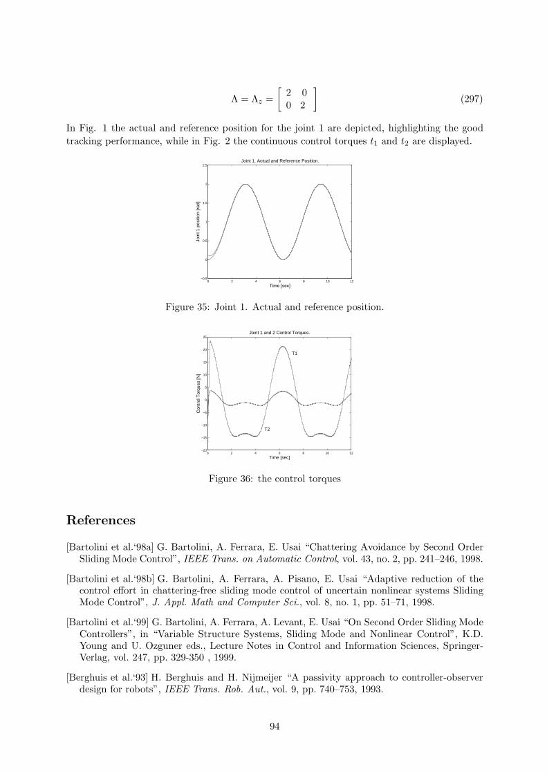
In Fig. 1 the actual and reference position for the joint 1 are depicted, highlighting the good

tracking performance, while in Fig. 2 the continuous control torques t1 and t2 are displayed.

0 2 4 6 8 10 12−0.5

0

0.5

1

1.5

2

2.5

Time [sec]

Join

t 1 p

ositi

on [r

ad]

Joint 1. Actual and Reference Position.

Figure 35: Joint 1. Actual and reference position.

0 2 4 6 8 10 12−20

−15

−10

−5

0

5

10

15

20

25

Time [sec]

Con

trol

Tor

ques

[N]

Joint 1 and 2 Control Torques.

T1

T2

Figure 36: the control torques

References

[Bartolini et al.‘98a] G. Bartolini, A. Ferrara, E. Usai “Chattering Avoidance by Second OrderSliding Mode Control”, IEEE Trans. on Automatic Control, vol. 43, no. 2, pp. 241–246, 1998.

[Bartolini et al.‘98b] G. Bartolini, A. Ferrara, A. Pisano, E. Usai “Adaptive reduction of thecontrol effort in chattering-free sliding mode control of uncertain nonlinear systems SlidingMode Control”, J. Appl. Math and Computer Sci., vol. 8, no. 1, pp. 51–71, 1998.

[Bartolini et al.‘99] G. Bartolini, A. Ferrara, A. Levant, E. Usai “On Second Order Sliding ModeControllers”, in “Variable Structure Systems, Sliding Mode and Nonlinear Control”, K.D.Young and U. Ozguner eds., Lecture Notes in Control and Information Sciences, Springer-Verlag, vol. 247, pp. 329-350 , 1999.

[Berghuis et al.‘93] H. Berghuis and H. Nijmeijer “A passivity approach to controller-observerdesign for robots”, IEEE Trans. Rob. Aut., vol. 9, pp. 740–753, 1993.

94

[Young et al.(eds.)‘98] K.D. Young and U. Ozguner (eds.)“Variable Structure Systems, SlidingMode and Nonlinear Control”, Lecture Notes in Control and Information Sciences, Springer-Verlag, 1999.


[Levant ‘93] A. Levant “Sliding order and sliding accuracy in sliding mode control”, InternationalJournal of Control, vol. 58, pp. 1247–1263, 1993.

[Slotine and Li ‘91] J.J.E.Slotine, W. Li Applied Nonlinear Control, Prentice–Hall International,Englewood Cliffs, New Jersey, 1991.

[Slotine et al. ‘85] J.J.E.Slotine “The robust Control of Robotic Manipulators”, Int. J. Rob. Res.,vol. 4, N. 2, 1985.

[Spong and Vidyasagar‘89] M.W. Spong and M. Vidyasagar Robot Dynamics and Control, Wiley,New York.

[Tang ‘98] Yu Tang “Terminal Sliding Mode Control for Rigid Robots”, Automatica, vol. 34, 1,51-56, 1998.


[Zasadnisky et al. ‘98] M. Zasadnisky, E. Richard, F. Khelfi and M. Darouach “DisturbanceAttenuation and Trajectory Tracking via a Reduced-order Output Feedback Controller forRobot Manipulators”, Automatica, vol. 34, 12, pp.1539–1546, 1998.

95

7 Control of IM Motor drives

The induction motor (IM) is widely used in the industry, due to its reliability, maintenance-free

operation and relatively low cost. However, precise and fast control of the flux and of the speed

(or torque) is not simple to obtain, due to the complex multivariable nonlinear dynamics, to

the unavailability of the rotor electrical quantities and to the parameter variations that occur

during working conditions. Moreover, state and control constraints are to be taken into account

for technical and/or economical reasons relevant to the sizing of the control hardware.

Over the years, field-oriented control has been recognized as the algorithm that gives the best

dynamic performance to the IM drive . It is based on the de-coupling between the flux and

torque control, which may be obtained in a suitable rotating reference frame (d-q transforma-

tion) [Bose ‘86, Vas ‘92], but it assumes the perfect knowledge of both rotor flux and motor

parameters. As far as the rotor resistance is concerned, it is known that it may vary up to the

150% of its nominal value, due to rotor heating. This causes a de-tuning of the torque and flux

controllers, which can decrease the drive performance [Bose ‘86, Vas ‘92].

A number of approaches which exploit passivity properties to ensure ultimate boundedness

and asymptotic convergence [Espinoza-Perez and Ortega ‘95] or resort to adaptive techniques

to on-line estimate the unknown rotor resistance [Marino et al. ‘99] have been presented in the

literature to cope with such phenomena.

Variable structure systems exploit the most obvious and heuristic way to withstand the uncer-

tainty. In such systems the control immediately reacts to any deviation of the system from the

desired behavior, represented by a motion constrained on a proper manifold in the state space,

steering it back onto the manifold by means of a sufficiently energetic control effort. This idea

traduces in high-frequency switching control, which is a drawback in mechanical systems, due

to the chattering phenomenon [Utkin ‘93, Utkin et al. ‘99], but it does not cause any difficulty

when electric drives are controlled, since the on-off operation mode is the only admissible one

for power converters. Therefore, it seems reasonable to use variable structure control algorithms

that produces PWM-type control signals directly.

In this framework, variable structure systems can exploit their powerful features in terms of

high efficiency, simplicity and robustness, and the sliding mode control methodology has been

widely used for control and/or observation purposes [Utkin ‘93, Utkin et al. ‘99] [Sabanovic and

Izosimov ‘81] [Benchaib et al. ‘99, Sangwongwanish et al. ‘90].

In this paper we propose a combined first-second order sliding mode control scheme that, by

using the measured speed and currents only, guarantees that all the systems trajectories remain

close to the desired profile, assuming weak informations about the motor parameters and thus

resulting robust to their variations. In particular, some implementation issues are discussed,

and, finally, the behaviour of the control scheme in presence of rotor resistance variation has

been investigated by simulations, showing the good properties of robustness and efficiency of

the proposed controller.

The proposed approach results to be conceptually similar to that used for the control of ma-

nipulators; it is reported mainly to made self-contained the argument of this chapter, while the

main aim of the following treatment is to put into evidence the implementation issues relevant

to the use of 2-sliding control for the control of IM drives.

96

7.1 Problem formulation

Assuming linear magnetic behaviour, the idealized two-axis IM vector equation in the statorreference frame [Vas ‘92] can be expressed as

dθdt

= ωdωdt

= 1J(Te − TL)

dΦr

dt= M(ω)Φr + αrLmis

disdt

= −A[L2mαr + Lrrs]is −ALmM(ω)Φr

+ALrRvs

(298)

where is = [isa, isb]T , Φr = [φra, φrb]

T are the stator current and rotor flux space vector respec-

tively, vs = [vs1, vs2, vs3]T is the three-phase stator voltage vector, θ and ω are the rotor position

and speed. TL is the unknown load torque, while the electromagnetic torque Te is given by

Te =3

2

Lm

Lrp(isbφra − isaφrb) (299)

J is the rotor inertia, rr and rs are the rotor and stator resistances, αr = rr/Lr is the inverse

rotor time constant, Lm, Lr, Ls are the linkage, rotor and stator inductances respectively, p is

the pole pair number, A = 1/(LsLr − L2m) and

M(ω) =

[

−αr −pωpω −αr

]

R =

[

23 −1

3 −13

0 1√3

− 1√3

]

(300)

The main control objectives are:

1. To make one of the mechanical coordinates (position or speed) equal to a smooth reference

input;

2. To keep the rotor flux vector modulus within the region of linear magnetic behaviour and

good torque response.

These objectives are attained by constraining the system motion onto the intersection of suitable

manifolds in the state space.

The three independent control variables vs1, vs2, vs3 allow to reach a three-dimensional manifold,

and the additional degree of freedom can be used to satisfy some optimization criteria, such as

the minimization of the inverter switching frequency, the reduction of losses and so on. The

criterion we use is the requirement that the supply voltages form a three-phase balanced system

[Utkin ‘93, Utkin et al. ‘99, Sabanovic and Izosimov ‘81].

7.1.1 Sliding Manifold Design

Let θ∗ and ω∗ be the position and speed reference signals to track, respectively. Choose the

corresponding manifold as

s1 = (ω − ω∗) + c(θ − θ∗) c ≥ 0 (301)

where c = 0 for the speed control and c > 0, ω∗ = θ∗, for the position control.

97

For the flux control, the sliding variable is chosen as the difference between the flux modulus

and the nominal reference value, while a mean integral deviation criterion is used to control the

voltage balancement.

s2 = ΦrM − Φ∗rM (302)

s3 =

∫ t

0

∫ t

0(vs1 + vs2 + vs3) (303)

where ΦrM =√

φ2ra + φ2

rb is the rotor flux modulus.

Define the sliding vector s as

s =

s1s2s3

(304)

The attainment of the sliding behaviour on the manifold s = 0 guarantees the satisfaction of

the control objectives.

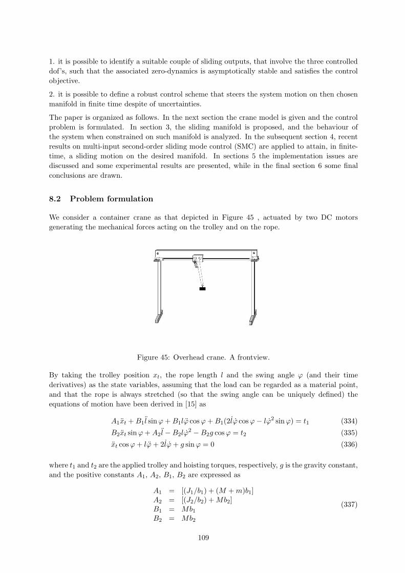
7.1.2 Controller Design

The relative degree between the sliding vector and the stator voltage vector is two, and the

relevant second order dynamics can be expressed as

y1 = sy1 = y2

y2 = Fy(·) + D(Φr)vs

(305)

where

Fy =

f1y(·)f2y(·)

0

D =

[

D1

1 1 1

]

(306)

f1y(·) = −AJ

(rrLs + rsLr)Te −3A

2JLmp

2ω(ΦraΦsa + ΦrbΦsb)

+1

J(c− b

J)(Te − Tr − bω)

1

JTr − (ω∗ + cω∗)

f2y(·) = −αr(1 +AL2m)ΦrM +

1

ΦrM

[

pω(ΦraΦrb − ΦrbΦra)

−rrrsLmA(Φraisa + Φrbisb)] − Φ∗

rM +1

ΦrM

(Φ2ra + Φ2

rb − Φ2rM )

(307)

D1 =

[

−k1Φrb d12 d13

k2Φra d22 d23

]

(308)

d12 = k1(12Φrb +

√3

2 Φra)

d13 = k1(12Φrb −

√3

2 Φra)

d22 = k2(−12Φra +

√3

2 Φrb)

d23 = k2(−12Φra −

√3

2 Φrb)

(309)

98

k1 = AJ Lmp k2 = 2

3rr

‖Φr‖LmA (310)

The expression for the stator flux Φs = Φsa + jΦsb is directly derived by combining the well

known formulasΦr = Lrir + LmisΦs = Lris + Lmir

(311)

Make the following assumptions:

H1. The electromechanical parameters of the motor belong to a known compact set.

H2. The state variables of the motor evolve within a compact subset in the state space.

If the motor parameters belong to some proper compact set, and the reference speed profile

is sufficiently smooth, then the entries of the vector Fy are bounded during normal operating

conditions, in which all the state variables are bounded. These assumptions are commonly

verified in practice. Moreover, matrix D can be proved to be nonsingular [Utkin ‘92, Utkin ‘93,

Utkin et al. ‘99].

The proposed strategy can be summarized as follows:

1. Consider an auxiliary dynamic system constituted by a double vector integrator with output

z1 and input w to be defined

z1 = z2

z2 = w(312)

2. Put

ε1 = s − z1 (313)

and consider the associated second order dynamics

ε1 = ε2ε2 = s− w

(314)

which consists of 3 non-interacting single-input systems controlled by means of the i− th entry

of the vector w.

3. Steer ε1 and the unmeasurable ε2 to zero by means of a suitable discontinuous control w. This

task can be accomplished by using the sub-optimal second order sliding mode control algorithm.

Once step 3 is performed, system (314) is said to evolve in accordance with a “second or-

der sliding mode” (2-SM) behaviour. The main theoretical properties of this special class of

sliding modes have been thoroughly investigated in [Levant ‘93, Bartolini et al. ‘99], while in

[Bartolini et al. ‘98b] it has been evidenced that the equivalent control for a 2-SM on the mani-

fold σ = σ = 0 (namely, the “second order sliding set”) can be defined as the continuous control

that solves the equation

σ = 0 (315)

As for the behaviour of the dynamical system (312), after the 2-SM on ε1 = ε2 = 0 has been

established, it can be analyzed by replacing the discontinuous control w with the corresponding

equivalent control, which, according to the above definition, by (305) and (315), is given by

weq = Fy(·) + D(Φr)vs (316)

99

The Filippov equivalent solution of the auxiliary system (312) can be therefore represented as

z1 = z2

z2 = weq = Fy(·) + D(Φr)vs(317)

The equivalent system (317), with measurable state variables z1 and z2, can be stabilized by

first order sliding mode control technique. Therefore, the fourth step of the proposed procedure

is

4. Define the sliding quantity

sz = z2 + Λzz1 (318)

where Λz is a positive definite diagonal matrix and steer the system (317) onto the manifold

sz = 0 by discontinuous control vs.

It is noteworthy that the simultaneous satisfaction of conditions

ε1 = ε2 = 0sz = 0

(319)

ensures the exponential convergence of vector s to zero

7.1.3 The Flux Observer

The reduced-oder observer proposed in [Damiano et al. ‘99], which is derived from a specific

Luenberger-type one [Verghese and Sanders ‘88] by suitably modifying the prediction error term

in order to obtain a semi-infinite stability range for the gain matrix entries, has been used for

the implementation of the control law.

The observer dynamics is given by

h =[

I + Lm

LrK]

[−αrI + ωJ] Φr

+αrLmis + K[

(rs + αrL2

m

Lris − vs)

]

Φr = h + KσLsis

(320)

where I and J are the 2-by-2 identity and unit rotation matrixes respectively, i.e.

I =

[

1 00 1

]

J =

[

0 −11 0

]

(321)

σ = 1−L2m/LsLr is the leakage coefficient and the matrix K is the gain matrix to be defined in

order to ensure stability and fast decay of the tracking error. Taking the K matrix as K = kI,

it can be proved, by using as a Lyapunov candidate function the square norm of the tracking

error, that the stability range for the k parameter is the semi-infinite set(

− Lr

Lm,∞)

, and that

the error rate decay arbitrarily increases as k tends to infinity. In [Damiano et al. ‘99] the

robustness analysis of the proposed observer against the rotor resistance variation has been

briefly performed, showing the ultimate boundedness of the error in case of a bounded variation

of resistance, and its inverse proportionality with respect to the gain k.

100

7.2 The control Algorithm

The overall proposed controller is summarized in the following

Proposition 1:

Consider system (298),(300), satisfying assumptions H1-H2, and let the quantities s and sz be

defined according to (301)-(304),(312),(318).


vsi = −VMsign(s∗zi) (322)

wi = WMisign(ε1i −

1

2ε1iM ) (323)

where i = 1, 2, 3, s∗z = DT sz, ε1 and ε1iM are defined according to (313) and (327), the bus voltage

VM and the constants WMi, (i=1,2,3), are defined according to (333) and (326) respectively,

ensures the local asymptotic convergence to zero of the components of the vector s.

Proof.

Part I: Stabilization of system (314)

The drift term s of system (314) takes the form

s = Fy(·) + D(Φr)vs (324)

Under assumptions H1-H2, the entries si, i = 1, 2, 3, of the vector s can be upper bounded by

known constants, in accordance with

|si| ≤ ΥMi (325)

The three non-interacting subsystems in which can be decomposed system (314), each one with

drift term si and control wi, fall in the class of plants that can be stabilized in finite time by using

the sub-optimal 2-SMC algorithm [Bartolini et al. ‘98a, Bartolini et al. ‘99], and the finite-time

stabilization of all entries of vectors s and s can be attained by suitable discontinuous control

w, provided that the control amplitudes are chosen according to

WMi> 2ΥMi (326)

A precise evaluation of the constants ΥMi can be found exploting assumptions H1 and H2. It

must be underlined that the exact knowledge of such bounds is not useful, as it is, in general,

highly conservative. Simulation show that effectiveness of the control scheme is obtained even

by using control values much smaller than the sufficient theoretical ones.

The switching logic of the sub-optimal algorithm is clarified for the reader’s convenience. The

term ε1Mi (i = 1, 2, 3) in (323) represents the last singular value of εi1, according to

εMi(t) =

εi(0) 0 ≤ t < tM1

εi(tMk) tMk

≤ t < tMk+1

tMks.t. εi(tMk

) = 0 k = 1, 2, . . .

(327)

An algorithm for the approximate detection of the singular points has been presented in [Bartolini et al. ‘98a].

101

Part II: Stabilization of the equivalent system (317)

To prove that the control vs forces sz to converge to zero in finite time, following the same

guidelines in [Utkin ‘93, Utkin et al. ‘99], consider the following Lyapunov function candidate

Vz =1

2sTz sz (328)

Taking into account that ε1 = ε2 = 0, its time derivative can be expressed as

Vz = sTz (Fy(·) + D(Φr)vs + Λz2) (329)

Substituting control (322) into (329) yields

Vz = s∗zTFy

∗ − VM |s∗z| (330)

where

Fy∗ = (D−1Fy)T (331)

As a consequence of assumptions H1 and H2, relying on the fact that the matrix D is nonsingular,

the entries of the vector Fy∗ can be upper bounded by proper constants according to

|Fy∗i | ≤ F ∗

yi i = 1, 2, 3 (332)

The condition

VM > maxi F∗yi (333)

provide negativeness of Vz, hence the origin of the s∗z space is asymptotically stable. By virtue

of det(D) 6= 0, the sliding mode arises on the manifold s = 0 as well.

7.3 Implementation Issues

The proposed control law is discontinuos, hence it is well suited to be implemented by means

of power converters. No PWM seems to be necessary, as the control signal is already a pulse-

width-modulated signal. The bus voltage VM has to satisfy the inequality (333), and the state

of the switches of the inverter legs can be directly set by the VSC according to the switching

logic in (322). The problem of maintaining sufficiently high the switching frequency of the

control is crucial in this context. Due to the inertias of the measurement devices and/or to

the mechanical nature of some sliding quantities, the switching frequency of the control may be

significantly smaller than typical PWM frequencies. This problem can be counteracted by using

state observers, which “inject” high frequencies in the feedback loop by means of the measured

electrical quantities used for the observer implementation [Utkin ‘92, Utkin ‘93, Utkin et al. ‘99].

In the proposed technique the high frequency dynamics of z (due to the discontinuos signal

w) gives to the sliding vector sz the harmonic content (something similar to the persistent

excitance condition in adaptive control) sufficient to establish a sliding regime characterized

by a sufficiently high switching frequency of the PWM input voltage. Moreover, computer

simulations show that, during the reaching phase and at every time instant at which the sliding

mode is not established, an unacceptable current peaking occurs, as a direct consequence of

102

the fact the no control switchings occur, and the motor is supplied with the bus voltage for a

long period of about some ms. To solve this problem, in the practical implementation of the

control law, an accurate planning of the reference trajectories is mandatory, in order

to establish the sliding mode from the initial time instant on. As a result, the supply voltage

immediately commutes at very high frequency, and the transient peaking of the stator currents

is avoided.


The proposed control algorithm has been simulated considering a commercial induction motor

drive. All parameters and ratings are given in Table I. The bus voltage is set to 500V . A speed

regulation test has been first performed, in which the reference speed is first the nominal speed

of the motor and then it is is reduced of the 50% . The flux exhibits a small oscillation around

the nominal value during the transient phases but it promptly comes to the desired value. In

Fig. 37 are reported the actual and desired speed profile, while in Fig. 38 is depicted the flux

modulus, which is wanted to be kept at the nominal value Φ∗rM = 0.7 Wb. The same test has

been repeated by varying the actual motor resistance to test the robustness of the observer-

controller structure. The actual resistance has been smoothly increased from the nominal value

in Table I up to the 150% (see fig. 39). The control system is quite insensitive to the resistance

variation, as it is evidenced in Figg. 40 and 41.

Secondly, the response of the system to a sinusoidal reference speed has been investigated. Unlike

the previous test, a perfect speed tracking is achieved, due to the smooth profile of the reference

speed (see Fig. 42). After the first reaching transient, the sliding mode is never lost, and the

slight transient oscillation of the flux modulus, highlighted in Fig. 38 for the regulation test,

disappears, as it can be seen in Fig. 43.

0 0.02 0.04 0.06 0.08 0.1 0.12 0.14 0.16 0.18 0.2−20

0

20

40

60

80

100

120

140

160

Time [sec]

Spe

ed [r

ad/s

ec]

Figure 37: Speed regulation. Actual and reference speed.

Now we want put into evidence the basic issues relevant to the planning of the reference trajec-

tories for the sake of reducing the current peaking. Making refrence to the problem of regulating

the speed along some constant value, instead of step references for speed and flux we use we

use smooth interpolations between the zero speed and the final desired value. In Fig. 44 can

be noted the perfect matching between the reference and actual speed if a smooth profile is

used, and also the capability of directly controlling the amplitude and the slew rate of the stator

current during the transient must be pointed out.

103

0 0.02 0.04 0.06 0.08 0.1 0.12 0.14 0.16 0.18 0.20

0.1

0.2

0.3

0.4

0.5

0.6

0.7

0.8

Time [sec]F

lux

[Wb]

Figure 38: Speed regulation. The actual flux modulus.

0 0.05 0.1 0.15 0.2 0.250.9

1

1.1

1.2

1.3

1.4

1.5

Time [sec]

r r [Ω]

Figure 39: Speed regulation with rotor resistance variation. The rotor resistance.

0 0.05 0.1 0.15 0.2 0.250

20

40

60

80

100

120

140

160

Time [sec]

Spe

ed [r

ad/s

ec]

Figure 40: Speed regulation with rotor resistance variation. Actual and reference speed.

0 0.05 0.1 0.15 0.2 0.250

0.1

0.2

0.3

0.4

0.5

0.6

0.7

0.8

Time [sec]

Flu

x [W

b]

Figure 41: Speed regulation with rotor resistance variation. The actual flux modulus

104

0 0.02 0.04 0.06 0.08 0.1 0.12 0.14 0.16 0.18 0.2−50

−40

−30

−20

−10

0

10

20

30

40

50

Time [sec]

Spe

ed [r

ad/s

ec]

Figure 42: Speed Tracking. Actual and reference speed.

0 0.02 0.04 0.06 0.08 0.1 0.12 0.14 0.16 0.18 0.20

0.1

0.2

0.3

0.4

0.5

0.6

0.7

0.8

Time [sec]

Flu

x [W

b]

Figure 43: Speed Tracking. The actual flux modulus.

0 0.02 0.04 0.06 0.08 0.1 0.12 0.140

20

40

60

80

100

120

140

160

Figure 44: The effect of the reference speed slope on the current transient peaking

105

Rating power 2.2kWRating torque 15NmRating speed 1410rpmPole pair 2Inertia constant 0.009kgm2

Damping coefficient 0.005NsStator resistance 0.8533ΩStator leakage inductance 0.005HMutual inductance 0.085HRotor resistance 0.95ΩRotor leakage inductance 0.005H

Table I: IM Parameters and Ratings

7.5 Summary

A new approach for the variable structure control of IM drives, which combines first and second

order sliding mode control strategies, is proposed in this paper. Robustness against parameter

uncertainty and/or their variation is obtained, as evidenced by simulations. No acceleration

observer must be implemented, therefore reducing the sensitivity to the load disturbance as

well. Further investigations will be devoted to test the performances of its digital realization

and to reduce the peaking of the currents, making it ready for experimental verifications of the

good simulation results.

References

[Bartolini et al. ‘98a] G. Bartolini, A. Ferrara, E. Usai “Chattering Avoidance by Second Order

Sliding Mode Control”, IEEE Trans. on Automatic Control, vol. 43, no. 2, pp. 241–246, 1998.




Verlag, vol. 247, pp. 329-350 , 1999.

[Bartolini et al. ‘98b] G. Bartolini, A. Ferrara, A. Pisano, E. Usai “Adaptive reduction of the

control effort in chattering-free sliding mode control of uncertain nonlinear systems Sliding

Mode Control”, J. Appl. Math and Computer Sci., vol. 8, no. 1, pp. 51–71, 1998.

[Benchaib et al. ‘99] A. Benchaib et al. “Real-Time Sliding-Mode Observer and Control of an

Induction Motor”, IEEE Trans. on Ind. Electronics, 46, 128–137 (1999).

[Bose ‘86] B.K. Bose Power Electronics and AC Drives, Englewood Cliffs, NJ, Prentice Hall,

(1986).

[Damiano et al. ‘99] A. Damiano, G. Gatto, I. Marongiu A. Pisano “Synthesis and Digital Im-

plementation of a Reduced Order Rotor Flux Observer for IM drive”, Proc. of the IEEE Int.

Symp. on Industrial Eletronics ISIE 99, Bled, Slovenia, pp. 729–734 June 1999.



106

[Marino et al. ‘99] R. Marino, S. Peresada, P. Tomei, “Global Adaptive Output Feedback Con-

trol of Induction Motors with Uncertain Rotor Resistance”, IEEE Trans. on Aut. Control,

44, 967–983 (1999).

[Espinoza-Perez and Ortega ‘95] G. Espinoza-Perez, R. Ortega, “An Output Feedback Globally

Stable Controller for Induction Motors”, IEEE Trans. on Aut. Control, 40, 138–143 (1995).

[Sabanovic and Izosimov ‘81] A. Sabanovic, D. Izosimov, “Applications of Sliding Modes to In-

duction Motor Control”, IEEE Trans. on Industry Applications, 17, 41–49 (1981).

[Sangwongwanish et al. ‘90] S. Sangwongwanish et al., “Desing of Sliding Observers for Robust

Estimation of Rotor Flux of Induction Motors ” Proc. of the Int. Power Electr. Conf. IPEC

90, Tokyo, Japan, pp. 1235–1242, 1990.

[Utkin ‘92] V.I. Utkin Sliding Modes In Control And Optimization, Springer Verlag, Berlin,

(1992).

[Utkin ‘93] V.I. Utkin “Sliding Modes Control Design Principles and Applications to Electric

Drives”, IEEE Trans. on Ind. Electronics, 40, 23–35 (1993).

[Utkin et al. ‘99] V.I. Utkin et al. Sliding Modes Control in Electromechanical Systems, Taylor

and Francis, London, 1999.

[Vas ‘92] P. Vas, Vector Control of AC Machines, Oxford Science Publications, (1992).

[Verghese and Sanders ‘88] G. Verghese, P. Sanders, “Observers for Flux Estimation in Induction

Machines”, IEEE Trans. on Ind. Electronics, 35, 85–94 (1988).

107

8 Control of Container Cranes

8.1 Introduction

An interesting and challenging applicative test for advanced control techniques is constituted

by the control of cranes. In many industrial as well as civil engineering environments, safety

constraints and economical reasons require that the transfer of heavy loads over long distances

is executed minimizing the load oscillation and the operation time.

Inspired from the behaviour of expert crane drivers, the control strategy has been often designed

in two-stages: off-line path planning, in accordance with some optimization criteria, and on-line

path tracking. In particular, optimal control techniques have been widely used to address the

problem of the path planning [Auernig and Troger ‘87, 6, 10, 15]. The reference trajectories were

chosen to minimize some specific indexes, linked to the swing angle and its derivative [15], or to

the energy consumption, which is claimed to be meaningful with respect to system stresses such

as oscillations and non-smooth motions [10]. Nevertheless, the high sensitivity of the resulting

open-loop strategies to parameter mismatching and external disturbances has been pointed out

in the literature [21].

A linear, parameter-varying, crane model can be obtained by means of a suitable time-scaling [18,

20], that allows for the use of adaptive pole-placement control techniques [19], gain-scheduling

[7] or Lyapunov-equivalence-based observer/controller design [8].

The usual goal is to achieve zero swing only at the end of the transport. However, swing during

transport may bee too large. In [14] this fundamental consideration was pointed out, and an

effective approach to obtain the swing suppression also during load motion was presented, which

requires the perfect knowledge of the system’s parameters.

We address and solve the same problem assuming that the actual system parameters are uncer-

tain but belonging to a known compact domain, and also that the control torque are generated

by means of unmodeled actuators (DC drives with unknown parameters).

Due to model uncertainties, the use of robust control techniques is motivated. Variable structure

systems are well known to be robust and easy to implement [17]. A suitable manifold in the state

space is defined such that the system exhibits the desired behavior when constrained to evolve

on such a manifold. A control action is defined by a worst-case analysis to drive the system onto

the manifold despite of model uncertainties. As a result, the plant behavior becomes insensitive

to (and independent from) any uncertainties or disturbances that do not steer the plant outside

from the manifold

The actual case does not belong to the standard classes of problems dealt with by the sliding

mode control methodology; indeed, the overall system is under-actuated, since there are three

degrees of freedom (dof) to be controlled (the load coordinates and the swing angle) and only

two control actions (the motor voltages). Each dof is represented by a proper system output,

and the control objective is to make these outputs to exhibit the desired behaviour.

When the number of controlled dof is the same as the independent controls, a sliding manifold

could be chosen so that, in the constrained motion, the dynamics of the relevant system outputs

are decoupled. If we try to apply this logic to the problem under investigation, at least one dof

dynamics would result in being uncontrollable.

In this paper we succeed in proving that:

108

1. it is possible to identify a suitable couple of sliding outputs, that involve the three controlled

dof’s, such that the associated zero-dynamics is asymptotically stable and satisfies the control

objective.

2. it is possible to define a robust control scheme that steers the system motion on then chosen

manifold in finite time despite of uncertainties.

The paper is organized as follows. In the next section the crane model is given and the control

problem is formulated. In section 3, the sliding manifold is proposed, and the behaviour of

the system when constrained on such manifold is analyzed. In the subsequent section 4, recent

results on multi-input second-order sliding mode control (SMC) are applied to attain, in finite-

time, a sliding motion on the desired manifold. In sections 5 the implementation issues are

discussed and some experimental results are presented, while in the final section 6 some final

conclusions are drawn.

8.2 Problem formulation

We consider a container crane as that depicted in Figure 45 , actuated by two DC motors

generating the mechanical forces acting on the trolley and on the rope.

Figure 45: Overhead crane. A frontview.

By taking the trolley position xt, the rope length l and the swing angle ϕ (and their time

derivatives) as the state variables, assuming that the load can be regarded as a material point,

and that the rope is always stretched (so that the swing angle can be uniquely defined) the

equations of motion have been derived in [15] as

A1xt +B1 l sinϕ+B1lϕ cosϕ+B1(2lϕ cosϕ− lϕ2 sinϕ) = t1 (334)

B2xt sinϕ+A2 l −B2lϕ2 −B2g cosϕ = t2 (335)

xt cosϕ+ lϕ+ 2lϕ+ g sinϕ = 0 (336)

where t1 and t2 are the applied trolley and hoisting torques, respectively, g is the gravity constant,

and the positive constants A1, A2, B1, B2 are expressed as

A1 = [(J1/b1) + (M +m)b1]A2 = [(J2/b2) +Mb2]B1 = Mb1B2 = Mb2

(337)

109

in which M and m are the total masses of the container and of the trolley, respectively, J1 and

J2 are the total inertia of brake, drum and reduction gears of the trolley motor (TM) and of

the hoist motor (HM) drives, respectively, b1 and b2 represent the equivalent TM and HM drum

radius, reduced to the motor side.

The actuator dynamics can be represented as

Π1t + Π2t = v − Π3r (338)

where v = [v1 v2]T is the vector of the motor supply voltages, t = [t1 t2]

T , r = [xt l ]T and the

diagonal matrixes Πi, i = 1, 2, 3, are given by

Π1 =

[

l1/kt1 00 l2/kt2

]

Π2 =

[

r1/kt1 00 r2/kt2

]

Π3 =

[

ke1/b1 00 ke2/b2

]

(339)

where r1 (r2) is the TM (HM) resistance, l1 (l2) is the TM (HM) inductance, kt1 (kt2) is the

TM (HM) torque constant and ke1 (ke2) is the TM (HM) back-emf constant.

The control objective is to move the load along a pre-specified trajectory as faster as possible,

while keeping the swing angle sufficiently small. Assume that the crane and motor parameters

are uncertain but belonging to a known compact set.

The control problem is challenging for many reasons: the system is nonlinear, highly coupled,

uncertain and underactuated (three output variables must be controlled by using two control

actions). The goal is to move the load from the initial position (xi, yi) to a final, desired, location

(xf , yf ) along a pre-specified path, while keeping the load oscillation as small as possible.

As the rope is assumed always stretched, the load coordinates depend on the system’s state as

followsx = xt + lsinϕy = lcosϕ

(340)

Often [15, 10] the overall loading and unloading motion of the suspended mass is divided in three

different phases which are separately dealt with: the vertical motion (pure load hoisting and

lowering), the transversal motion and the horizontal one (Fig. 2). Apart from the pure vertical

motion, which does not cause load oscillations, any generic motion task can be characterized

by load oscillation, which must be kept as small as possible during the load transport and

suppressed at the end of the transfer.

We distinguish two phases: the “traveling phase”, including the whole travel of the load to-

ward the final location, and the “arrival phase”, activated as soon as a suitable vicinity of the

destination point is reached, in which the load must be stabilized on the final location.

We propose a control strategy that is able to guarantee, for each type of load movement,

(transversal, horizontal and vertical) the robust tracking of the desired path and, at the same

time, the active damping of the load oscillations.

Generally, in the previously quoted literature, the load is forced to track the desired path with

an off-line designed velocity profile, with no feed-back on the swing angle. In the actual case,

the swing suppression is obtained on-line by constraining the system’s motion on a suitable

manifold which involves both the desired path and the swing angle. Roughly speaking, the

velocity is modified on-line, on the basis of the actual swing angle, to obtain the suppression of

the oscillations not only at the end of the transport but during transfer as well.

110

8.3 Sliding manifold design for trajectory tracking and oscillation damping

The design of a sliding-mode control system consists of two-steps. The first step is the choice of a

manifold in the state space such that, once the state trajectory is constrained on it, the system

behaviour, described by its zero dynamics with respect to the corresponding sliding outputs,

exhibits the desired performances. The second step consists of the design of control actions

capable of forcing the system state, after a finite transient time to evolve on the chosen manifold

(accordingly called sliding manifold).

In the actual case, since the control torques are not directly manipulable due to the actuator

dynamics, any sliding output of the type

s(q) = 0 (341)

where q = [xt , xt , l , l , ϕ , ϕ]T is the crane state vector has relative degree two, since the

actual control vector v acts on the second derivative of s. On the basis of these considerations,

the use of second order sliding modes appears to be sensible and motivated.

The present chapter deals with the first step of the control design procedure, i.e. the design of

the sliding manifold and the stability analysis of the zero-dynamics, while the presentation of

the control technique guaranteeing the attainment of the sliding motion is postponed to Section

4, in which recent results on multi-input second-order sliding mode control are recalled and

applied to the actual control problem.

In the case under investigation, three dof must be controlled by using two independent control

actions. Of course, independent tracking of the three associated system’s outputs is impossible,

but a mixed objective of tracking for two variables, and stabilization for the remaining one, can

be attained in principle,

The choice of a suitable sliding manifold is the most critical point of the controller design. When

constrained onto the manifold, the system dynamics (zero-dynamics, [9]) must exhibit the desired

path tracking performance, while the stability of the swing dynamics must be guaranteed as well.

If the swing angle were not an issue, it would be possible to define the sliding output vector as

s(q) =

[

s1s2

]

=

[

xt − xdt + c1(xt − xd

t )

l − l d + c2(l − l d)

]

(342)

where c1, c2 are positive constants and the superscript ′d′ indicates the desired behaviour.

On the manifold s = 0, the exponential tracking of the desired path is achieved.

As for the analysis of the system’s zero dynamics, we refer to the approximate model suggested

in [15], valid for small load oscillations. More precisely, we assume that the the load swing angle

is so small that all terms containing ϕαϕβ (α ≥ 0, β ≥ 0, α + β ≥ 2) can be neglected, and the

approximations cos(ϕ) ≈ 1 and sin(ϕ) ≈ ϕ hold.

The above approximations yield the following model

xt = δ1gϕ+ z1 − δ1ϕz2 (343)

l = −δ2ϕz1 + z2 (344)

111

ϕ = −1

l

[

(1 + δ1)gϕ + 2lϕ]

− 1

lz1 +

δ1lϕ z2 (345)

where z1 and z2 are new control variables defined as

z1 = b1J1+mb2

1

t1 z2 = b2(t2+Mb2g)J2+Mb2

2

(346)

and δ1, δ2 are the positive constants

δ1 =Mb21

J1+mb21

δ2 =Mb22

J2+Mb22

(347)

The zero-dynamics of the swing angle can be obtained substituting z1 and z2 in (345) with those

keeping to zero the outputs s1 and s2. Intuitively, such input zeq = [z1eq z1eq ] (which is referred

in the VSS community as “equivalent control”) is the solution of the system

s = 0 (348)

Differentiating (342), and considering (343)-(347) and (348), after some manipulations one ob-

tains

z1eq = −δ1(g − l)ϕ+ kϕ+ xdt − c1(xt − xd

t )

z2eq = δ2[xdt − c1(xt − xd

t )]ϕ

(349)

Accordingly, the swing angle zero-dynamics turns out to be given by

ϕ = − g

l(t)ϕ− 2l(t)

l(t)ϕ− 1

l(t)[xd

t − c1(xt − xdt )] (350)

The stability of the above time-varying dynamics is strongly affected by the operating conditions,

and it is very difficult to predict the actual system’s behaviour. Indeed, also the frozen models

may be unstable, depending on the actual movement performed by the load. The above zero

dynamics can be considered as uncontrollable, in the sense that its stability is influenced by the

sign of l and no control action seems to be available to ensure it.

The main idea proposed in this paper is to add a swing-dependent term in the definition of s1,

i.e. we propose to define the following sliding outputs

s1 = xt − xdt + c1(xt − xd

t ) − kϕ

s2 = l − l d + c2(l − l d)(351)

where k is a positive constant.

It is not difficult to verify that the zero-dynamics turns out to be modified as follows

ϕ = − g

l(t)ϕ− k + 2l(t)

l(t)ϕ− 1

l(t)[xd

t − c1(xt − xdt )] (352)

i.e. an artificial viscous damping proportional to kl−1(t) appears in the swing’s zero dynamics. It

is reasonable to argue that the increase of k could have a stabilizing effect on the zero dynamics,

and this intuitive property is formalized in the next subsections.

112

8.3.1 The traveling phase

Let the desired path be expressed as

l d = f(xt) (353)

In order to better explain our proposal, the procedure will be detailed making reference to a

parabolic reference trajectory (Fig. 46 ), i.e.

l d = l0 + Γx2t |xt| ≤ XM (354)

l0

XM-XM xt

l

Figure 46: The parabolic reference path.

Consider the following two-dimensional sliding manifold

s′

1 = xt − V0 − kϕ

s′

2 = l − ld + c2(l − f(xt))(355)

where V0 is a positive constant that represents the desired horizontal speed, the desired rope

velocity ld can be obtained, by differentiating (354), as

ld =df

dxtxt = 2Γxtxt (356)

The requirements regarding the trolley position and the swing angle should be satisfied by

keeping the equality s′

1 = 0. Note that s′

1 contains both the trolley velocity and the swing angle.

The stabilizing effect of the k parameter (see (352)) can be first exploited to stabilize around

the origin the nonlinear swing angle dynamics, so that the term ϕ in (355) vanishes, and, on

s′

1 = 0, the trolley turns out to move with the desired velocity V0.

The manifold s′

2 = 0 is designed to ensure that, for each current value of xt, the rope length is

adjusted in order to maintain the load on the desired trajectory f(xt).

In the actual case, when constrained onto the two-dimensional manifold s′

1 = s′

2 = 0 , the

original 6th-order system is reduced to a 4th-order plant, which must be proved to enjoy the

desired properties of tracking and stability.

113

By considering (355) and (352), the actual system’s zero-dynamics turns out to be

xt = V0 + kϕ (357)

ϕ = − g

l(t)ϕ− k + 2l(t)

l(t)ϕ (358)

l = ld − c2(l − ld) (359)

Note that the third equation is independent from the others, while the first two equations are

coupled with the remaining ones.

In order to simplify the stability analysis, we regard the second order swing dynamics (358) as

a linear, autonomous, parameter-varying, system, and our objective is to show that a suitably

chosen k parameter guarantees the asymptotic stability.

Using the time-dependent Lyapunov-candidate function

V (ϕ, ϕ, t) =1

2

g

l(t)ϕ2 +

1

2ϕ2 (360)

one obtains

V (·) = −k + 2l(t)

l(t)ϕ2 − 1

2

gl(t)

l2(t)ϕ2 (361)

that, for any positive value of k, implies asymptotic stability if l > 0 (i.e. when the rope is

lenghtened). By virtue of the well known Barbalat’s Lemma (see [16]), one can assess the swing

angle asymptotic stability also if the rope length is kept constant (l = 0, pure horizontal load

motion).

To obtain a more general stability result, valid whatever the sign of l is, consider the following

auxiliary variable

w = ϕ+ cϕ c > 0 (362)

where c is a positive arbitrary constant.

Note that on the manifold s′

2 = 0, after an exponential transient, the rope length and its

derivative will coincide with the desired values in (354) and (356), so that, by considering (357)

and (359), and neglecting, by assumption, the resulting term that contains ϕϕ , (358) can be

rewritten as

ϕ = −a(ξ)ϕ− b(ξ)ϕ (363)

where ξ represents the actual trolley position and

a(ξ) =g

l0 + Γξ2(364)

|ξ| ≤ XM (365)

b(ξ) =k + 4V0Γξ

l0 + Γξ2(366)

114

In the new w-ϕ coordinates, (358) can be rewritten as

ϕ = −cϕ+ ww = − [b(ξ) − c]w + [γ(ξ) − a(ξ)]ϕ

(367)

where

γ(ξ) = c(b(ξ) − c) (368)

Trivially, the asymptotic stability of system (367)-(368) implies that of system (358).

Define the following Lyapunov candidate function

V (ϕ,w) =1

2ϕ2 +

1

2w2 (369)

whose derivative V is a quadratic form of the type

V (·) = −[ϕ , w]T M(ξ)[ϕ , w] (370)

where

M(ξ) =

[

c −γ(ξ)−a(ξ)+12

−γ(ξ)−a(ξ)+12 b(ξ) − c

]

(371)

In order to ensure that the matrix M(ξ) is positive definite, the inequality

4γ(ξ) > [γ(ξ) − a(ξ) + 1]2 (372)

must be verified for each admissible value of ξ.

Note that the parameter c is absolutely fictitious, as it appears only in the stability proof and

does not affect in any way the structure of the sliding manifold and of the controller.

Moreover, note also that, thanks to the introduction of such artificial parameter, the stability

analysis of the time-varying system (358) can be easily performed by means of a Lyapunov

function that does not contain explicitly the time varying parameters.

After some algebraic manipulations, the solution of (372) can be derived as

g1(ξ) < γ(ξ) < g2(ξ) (373)

where

g1(ξ) = a(ξ) + 1 − 2√

a(ξ)

g2(ξ) = a(ξ) + 1 + 2√

a(ξ)(374)

The limiting curves g1(ξ) and g2(ξ) (reported in fig. 5for l0 = 10cm and Γ = 1m−2), depend

only on the reference path, while the actual crane parameters do not enter in this stability test.

115

By acting on k and c, the curve γ(ξ) must be “shaped” in order to lie within the limiting curves

g1(ξ) and g2(ξ) in the domain of interest. Note that, as ξ tends to ±∞, γ(ξ) tends to −c2, while

g1(ξ) and g2(ξ) tend to the unity. This means that the domain of stability will be always a finite

open interval (fig. 5).

The product kc defines the shape of γ(ξ) for “small” values of |ξ|, and by varying kc the curve

moves in the vertical direction. In Fig. 47 it is shown that different curves γ(ξ), obtained for

different values of c and k while their product is kept constant, are almost coincident.

The effect on γ(ξ) of reducing c, while keeping constant ck, is evident only far from the origin,

and traduces in “pulling up” the curve. This can be used to enlarge the domain of solution of

the inequality. The price to be payed is a reduced rate of decay for the swing angle.

As a design example, consider a desired path defined by l0 = .1m, Γ = 1m−1 and XM = 3, and

let the reference horizontal speed be V0 = 10cms−1.

First of all, we choose the product ck to place the maximum of γ(ξ) (i.e. γ(0)) approximately

at the medium between g1(0) and g2(0). Choosing c = 0.6 and k = 16.65 (ck ≈ 10) one obtains

the behaviour in Fig. 48 . Note that the actual curve γ(ξ) is entirely contained between the

limiting curves in the domain of interest |ξ| ≤ 3.

-2 -1.5 -1 -0.5 0 0.5 1 1.5 20

10

20

30

40

50

60

70

80

90

100

ξ [m]

c k = 10

c ∈ 0.5, 0.4, 0.3k ∈ 20, 25, 33.3

Figure 47: Different curves γ(ξ) with the same value of the product ck.

-3 -2 -1 0 1 2 3

0

20

40

60

80

100

120

g1(ξ)

g2(ξ)

γ(ξ)

Figure 48: c = 0.6 and ck = 10. The actual curves.

116

8.3.2 The arrival phase

As for the stabilization of the load around the desired final location, we use a different sliding

manifold, which is only devoted to a regulation task and relaxes any tracking objective.

Consider the following sliding outputs

s′′

1 = xt + c1(xt − xf ) − kaϕ

s′′

2 = l + c2(l − yf )(375)

where k, c1 and c2 are positive constants and xf , yf represent the final, desired, location.

Following the same procedure as in the previous subsection 3.1, it is not difficult to derive the

expression for the system zero dynamics as

xt = −c1(xt − xf ) + kaϕ (376)

l = −c2(l − yf ) (377)

ϕ = −g − c1ka

yfϕ− ka

yfϕ (378)

Around the final location, the swing dynamics is linear and stationary, and choosing

ka ∈ (0,g

c1) (379)

the asymptotic stability is trivially guaranteed.

It would be desirable to keep constant the value of k in both the traveling and arrival phases.

To this aim, one can choose k according to the stability requirements relevant to the traveling

phase, and then it is sufficient to set c1 sufficiently small to include the chosen k in the stability

domain (379).

8.4 A multi-input second-order sliding mode controller

In this section it is shown that the problem of steering the system motion on the desired manifold

can be solved, both in the travel phase and in the arrival phase, by means of a recently-proposed

multi-input second order sliding-mode control strategy [5].

Let qm = [xt xt l l ϕ ϕ] the state vector for the mechanical subsystem, and let q = [qTm tT ] be

the state vector for the whole electromechanical plant. Moreover, let pm be the column vector

containing the mechanical parameters and pe that containing the electrical ones, and define

p = [pTm pT

e ].

Successive differentiation of (355) and (375) yield

Travel phase Arrival phase

s′

= F′

1(qm,pm) + G(qm,pm)t

s′

= F′

2(q,p) + Π−11 G(q,p)v

s′′

= F′′

1(qm,pm) + G(qm,pm)t

s′′

= F′′

2(q,p) + Π−11 G(q,p)v

(380)

117

where s′

= [s′

1 s′

2]T , s

′′

= [s′′

1 s′′

2 ]T , F′

i(·) and F′′

i (·), i = 1, 2, are uncertain vector fields and

G(q,p) =1

A1A2 −Mb1 −MJcos2(ϕ)

[

A2 −Mb2sin(ϕ)−Mb1sin(ϕ) A1 −Mb2cos

2(ϕ)

]

(381)

is also uncertain but can be easily shown to be sufficiently dominant diagonal. This fact,

according to [5], is sufficient to express the multi-input control problem in a set of suitable,

almost decoupled, single-input second-order sliding mode control problems, without involving

any observer.

Furthermore, it is not difficult to verify that, if the reference path is sufficiently smooth, the

uncertain vectors F′

i(·) and F′′

i (·) (i = 1, 2) are norm-bounded in any bounded domain. This

means that, given any compact domain of interest in the state space, constant upperbounds F′

i

and F′′

i can be found such that

‖F ′

i (·)‖ ≤ F′

i i = 1, 2

‖F ′′

i (·)‖ ≤ F′′

i i = 1, 2(382)

Therefore, both in the travel phase and in the arrival phase, the sliding variable dynamics can

be stabilized by means of the sub-optimal second order sliding mode controller [1, 2].

The resulting control strategy consists of two stages, since the actual sliding manifold is modified

after the final location has been sufficiently approached according to the stability conditions

detailed in Sect. 3.1.

The control can be set as

vi = −β′

i(t)V′

i sign(s′

i(t) −1

2s′

i(T′

Mki)) i = 1, 2 (383)

until |xt−xf | > Σ, where the positive constant Σ represents the distance from the final position,

s′

i is defined in (354)–(355), and T′

Mkiare the time instants at which s

′

i , (i = 1, 2), is zero, V′

i ,

(i = 1, 2), are proper constants [5] and

β′

i(t) =

β′∗i if s

′

i(T′

Mki)(s

′

i(t) − 12s

′

i(T′

Mki)) > 0

1 if otherwise(384)

where β′∗i , (i = 1, 2), are proper constants [5]. After the vicinity |xt −xf | ≤ Σ has been reached,

the arrival phase is activated, and the definition of the sliding variable is modified according to

(375), where the positive coefficient c1 is chosen sufficiently small to include the actual value of k

within the stability domain (379). The resulting control strategy has still the form (383)-(384),

but considering s′′

i (t), V′′

i , β′′

i (t) and T′′

Mkiinstead of s

′

i(t), V′

i , β′

i(t) and T′

Mki, respectively.

The implementation of such controller guarantees the robust tracking of the desired path, and,

at the same time, the damping of the load oscillations during the whole load travel.

8.5 Implementation Issues and Experimental Results

First of all refer to a picture of the crane prototype (Fig. 54) and to a schematic diagram of the

digital experimental setup (Fig. 55).

118

The digital implementation of the proposed control scheme has been tested on a laboratory-sized

prototype built for experimental investigations. The sub-optimal second order SMC algorithm

has been shown to be robust against the sample-and-hold effect [3], so that the feasibility of the

digital implementation of the control law does not require further investigations. A sampling

period of Ts = .002s was used, and the acquired data have been on-line stored in the memory

of the PC and then off-line processed to make the graphics.

A load with mass of about 1 Kg is moved with a parabolic reference trajectory. The trolley and

rope velocities have been estimated by using real-time numerical differentiators based on second

order sliding modes [4]. A smooth transition between the travel phase and the arrival phase must

be performed to preserve the sliding behaviour. In Figures 49 and 50 the actual load coordinates,

and the swing angle versus time, are depicted, respectively. In a second experiment, an initial

oscillation is intentionally introduced, and the proposed controller has been implemented usinf

different values for the coefficient k, that corresponds to a “feedback gain” for the swing angle.

In particular, in a first test no-feedback action is performed on the swing angle (k = 0, see

Figure 51). Note that the oscillations propagates through the whole transfer of the load until

the destination point. Then, increasing values of k have been used and the oscillation is damped

faster and faster until the stability bound defined in section 8.3.2 is overcame. Using k = 80,

the actual trajectory remains close to the desired one, and the oscillation disappears before the

vertex of the actual trajectory is reached (k = 0, see Figure 52). In Figure 53 (corresponding to

the use of k = 640) it is evident the unstable behaviour of the swing angle in a vicinity of the

destination point.

0 5 10

0

20

40

60

80

100

Lo

ad

co

ord

ina

tes

[cm

]

Time [sec]

x

y

0 20 40 60 80

0

10

20

30

40

Lo

ad

ve

rtic

al p

os

itio

n [c

m]

Load horizontal pos ition [cm]

Figure 49: The actual and reference load coordinates.

0 5 10 15-0,10

-0,05

0,00

0,05

0,10

Sw

ing

Angl

e [ra

d]

Time [sec]

Figure 50: The actual swing angle.

119

0.1

−0.1 10 20 0

rad

Time [sec]

Figure 51: k=0. The propagation of the load oscillation.

0 20 40 60 80

0

10

20

30

40

Actual trajectory (solid line) and reference trajectory (dotted line)

Verti

cal l

oad

posi

tion

Horizontal load position

0 2 4 6 8 10-0,1

0,0

0,1

0,2

0,3

Sw

ing

angl

e [ra

d]

Time [sec]

Figure 52: k=80. The actual and reference load coordinates and the load swing.

rad

Time [sec]

Figure 53: k=640. The unstable behaviour of the swing angle.

120

Figure 54: Picture of the crane prototype.

xt

l

xt , l , ϕϕ(trolley and hoist motorpositions and swing angle)

vt , vl(trolley and hoistmotor voltages)

ϕ

Signal flux diagram

PC UNIT

The experimental setup

Figure 55: Schematic Diagram of the experimental setup

121

8.6 Conclusions

The problem of moving a suspended load using a container crane has been addressed and solved

by sliding-mode techniques. A suitable sliding manifold has been defined such that the system

motion, when constrained on such manifold, satisfy the control objectives, i.e. fast and accurate

load transfer and damping of the swing, both during the movement and at the end of the trans-

portation. The explicit dependence of the sliding manifold on the swing angle, that guarantees

the stability of the system’s zero dynamics, constitutes the main novelty of the present approach.

The use of the second order SMC methodology allows to take into account the unmodeled ac-

tuator dynamics, often neglected by other methodologies. Experimental investigations confirm

the good performance of the proposed method.

References

[Auernig and Troger ‘87] J.W. Auernig and H. Troger, “Time Optimal Control of Overhead

Cranes with Hoisting of the Load” Automatica, 23, 3, 437-447, 1987.

[1] G. Bartolini, A. Ferrara and E. Usai, “Chattering Avoidance by Second Order Sliding Mode

Control”, IEEE Trans. on Automatic Control, vol. 43, no. 2, 241–246, 1998.

[2] G. Bartolini, A. Ferrara, A. Levant and E. Usai, “On Second Order Sliding Mode Controllers”,

in Variable Structure Systems, Sliding Mode and Nonlinear Control, K.D. Young and U.

Ozguner (Eds.), Lecture Notes in Control and Information Sciences, Springer-Verlag, vol.

247, 329–350 , 1999.

[3] G. Bartolini, A. Pisano, E. Usai “Variable Structure Control of Nonlinear Sampled Data

Systems by Second Order Sliding Modes”, in Variable Structure Systems, Sliding Mode and

Nonlinear Control, K.D. Young and U. Ozguner (Eds.), Lecture Notes in Control and Infor-

mation Sciences, Springer-Verlag vol. 247, 43-68, (1999).

[4] G. Bartolini, A. Pisano and E. Usai, “First and Second Derivative Estimation by Sliding

Mode Technique” Journal of Signal Processing, 4, 2, 167–176, 2000.

[5] G. Bartolini, A. Ferrara, E. Usai and V.I. Utkin “On Multi-input second order sliding mode

control”, IEEE Trans. Aut. Contr., 45, 9, 1711-1717, 2000.

[6] J.W. Beeston, “Closed-loop time optimal control of a suspended load: a design study”, Proc.

4th IFAC World Congress, pp. 85-99, 1969.

[7] G. Corriga, A. Giua and G. Usai, “An Implicit gain-Scheduling Controller for Cranes”, IEEE

Trans. on Contr. Syst. Technology, 6, 1, 15–20, 1998.

[8] A. Giua, C. Seatzu, G. Usai,”Observer-controller design for cranes via Lyapunov equivalence”,

Automatica, 35, 4, 669–678, 1999.

[9] A. Isidori, Non Linear Control Systems, Springer Verlag, Berlin, 1989.

[10] J.J. Hamalainen, A. Marttinen, L. Baharova and J. Virkkunen, “Optimal path planning for

a trolley crane: fast and smooth transfer of the load”. IEE Proc. Control Theory Appl., 142,

1, 51–57, 1995.

122

[11] J. La Salle and S. Lefschetz, Stability by Liapunov’s Direct Method, Academic Press, London,

1961.

[12] A. Levant, “Sliding order and sliding accuracy in sliding mode control”, Int. J. of Control,

vol. 58, pp. 1247–1263, 1993.

[13] J. Levine, “Are there new industrial perspectives in the control of mechanical systems ?”,

Advances in Control - Highlights of ECC99, Paul M. Frank (Ed.), Springer-Verlag, London,

1999.

[14] K. Moustafa and A.M. Ebeid “Nonlinear Modeling and Control of Overhead Crane Load

Sway”, J. of Dyn. Syst. Meas. and Contr., Trans. ASME, vol. 110, pp. 266–271, 1988.

[15] A. Sakawa and Y. Shindo “Optimal Control of container cranes”, Automatica, vol. 18, No.3,

pp. 257–266, 1982.

[16] J.J.E.Slotine, W. Li Applied Nonlinear Control, Prentice–Hall International, Englewood

Cliffs, New Jersey, 1991.

[17] V.I. Utkin, Sliding Modes In Control And Optimization, Springer Verlag, Berlin, 1992.

[18] J. Virkkunen et al., “Computer control of overhead and gantry cranes”, Proc. 11th IFAC

world congress, Tallinn, Estonia, USSR, 401–405, 1990.

[19] J. Virkkunen et al., “Adaptive pole-placement control of a pilot crane”, Proc. 11th IFAC

world congress, Tallinn, Estonia, USSR, 313-318, 1990.

[20] A.S.I. Zinober, “The self-adaptive control of overhead crane operations”. Proc. 5th IFAC

Symp. On System Parameters Identification, Darmstad, 1161–1167, 1979.

[21] A.S.I. Zinober and A.T. Fuller, “The sensitivity of nominally time-optimal control systems

to parameter variation”, Int.J. of Control, 17, 673-703, 1973.

123

Date post:	04-Jul-2018
Category:	Documents
Upload:	phungminh
View:	214 times
Download:	0 times

Second Order Sliding Modes: Theory and Applications · INDEX Thesis’ overview Introduction and...

Documents