81
Chapter 10 Correlation and Regression Section 10-3 Correlation
| Date post: | 02-Jan-2016 |
| Category: |
Documents |
| Upload: | kermit-wyatt |
| View: | 26 times |
| Download: | 1 times |

Chapter 10Correlation and Regression
Section 10-3Correlation

Section 10-3
Exercise #13
Chapter 10Correlation and Regression

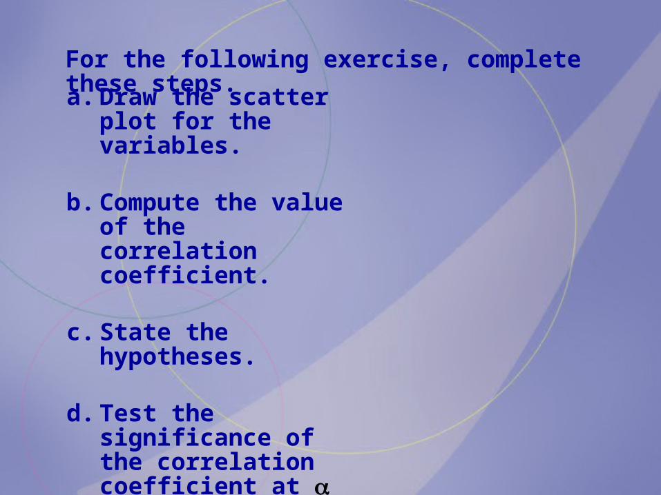
a. Draw the scatter plot for the variables.
b. Compute the value of the correlation coefficient.
c. State the hypotheses.
d. Test the significance of the correlation coefficient at = 0.05, using Table I.
e. Give a brief explanation of the type of relationship.
For the following exercise, complete these steps.

A researcher wishes to determine if a person’s age is related to the number of hours he or she exercises per week. The data for the sample are shown below.
Age x 18 26 32 38 52 59
Hours y 10 5 2 3 1.5 1
a. Draw the scatter plot for the variables.
2
4
6
810
0 10 20 3040 50 60Age
Hou
rs
70

b. Compute the value of the correlation coefficient.Age x 18 26 32 38 52 59
Hours y 10 5 2 3 1.5 1
y = 22.5
y2 = 141.25
n = 6
x = 225
x 2 = 9653
xy = 625

y = 22.5 y2 = 141.2 n = 6
x = 225 x 2 = 9653 xy = 625
– =
2 22 2 –
n xy x yr
n x x n y y

y = 22.5 y2 = 141.2 n = 6
x = 225 x 2 = 9653 xy = 625
– 6 625 225 22.5=
2 2 – –6 69653 225 141.25 22.5
r
r = – 0.832

0 1: = 0 and : 0H Hc. State the hypotheses.
Age x 18 26 32 38 52 59
Hours y 10 5 2 3 1.5 1

0 1: = 0 and : 0H H
d. Test the significance of the correlation coefficient at = 0.05, using Table I.
Age x 18 26 32 38 52 59
Hours y 10 5 2 3 1.5 1
n = 6 d.f . = 4 r = – 0.832
C.V . = ± 0.811
Decision: Reject H0 .

0 1: = 0 and : 0H H
e. Give a brief explanation of the type of relationship.
Age x 18 26 32 38 52 59
Hours y 10 5 2 3 1.5 1
n = 6 d.f . = 4 r = – 0.832
There is a significant linear relationship between a person’s age and the number of hours he or she exercises per week.
Decision: Reject H0 .

Section 10-3
Exercise #15
Chapter 10Correlation and Regression

For the following exercise, complete these steps.
a. Draw the scatter plot for the variables.
b. Compute the value of the correlation coefficient.
c. State the hypotheses.
d. Test the significance of the correlation coefficient at = 0.05, using Table I.
e. Give a brief explanation of the type of relationship.
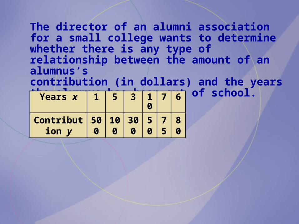
The director of an alumni association for a small college wants to determine whether there is any type of relationship between the amount of an alumnus’s contribution (in dollars) and the years the alumnus has been out of school. The data are shown here.
Years x 1 5 3 10 7 6
Contribution y 500 100 300 50 75 80

a. Draw the scatter plot for the variables.Years x 1 5 3 10 7 6
Contribution y 500 100 300 50 75 80
100
200
300
400500
0 2 4 86 10 20Years
Con
trib
utio
n
30
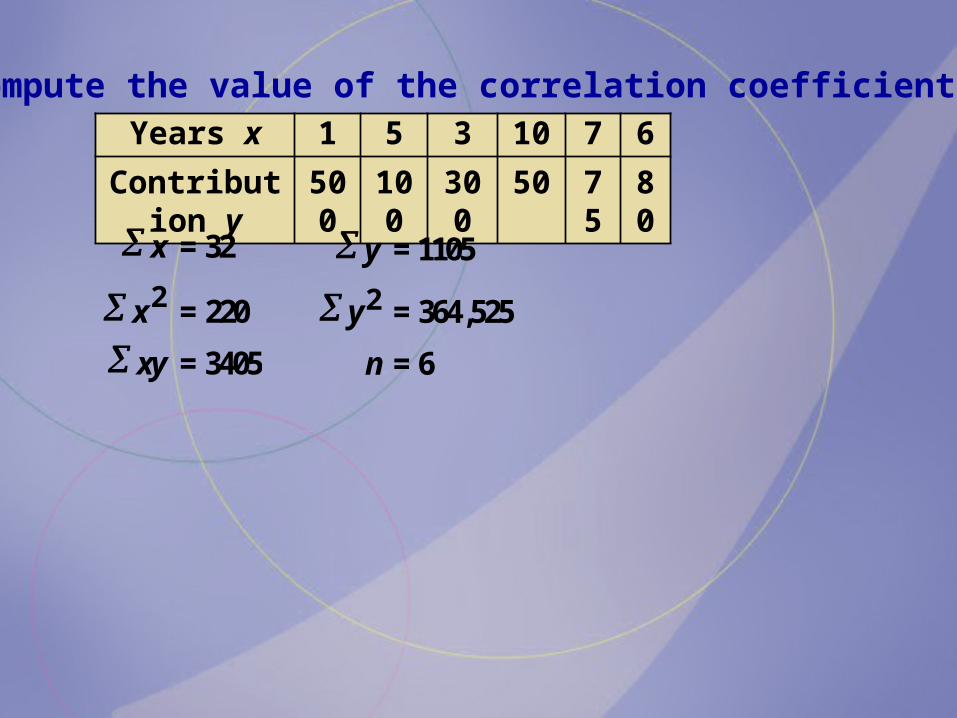
b. Compute the value of the correlation coefficient.Years x 1 5 3 10 7 6
Contribution y 500 100 300 50 75 80
y = 1105
y2 = 364,525
n = 6
x = 32
x 2 = 220
xy = 3405

b. Compute the value of the correlation coefficient.
y = 1105 y2 = 364,52 n = 6 x = 32 x 2 = 220 xy = 3405
– =
2 22 2 –
n xy x yr
n x x n y y

b. Compute the value of the correlation coefficient.
y = 1105 y2 = 364,52 n = 6 x = 32 x 2 = 220 xy = 3405
3405 – 32 11056=
2 2 6 220 – 32 364,525 – 11056
r
r = – 0.883

c. State the hypotheses.
0 1: = 0 and : 0H H
Years x 1 5 3 10 7 6
Contribution y 500 100 300 50 75 80

d. Test the significance of the correlation coefficient at = 0.05, using Table I.
Years x 1 5 3 10 7 6
Contribution y 500 100 300 50 75 80
0 1: = 0 and : 0H H
n = 6 d.f . = 4 r = – 0.883
Decision: Reject H0 .
C.V . = ± 0.811
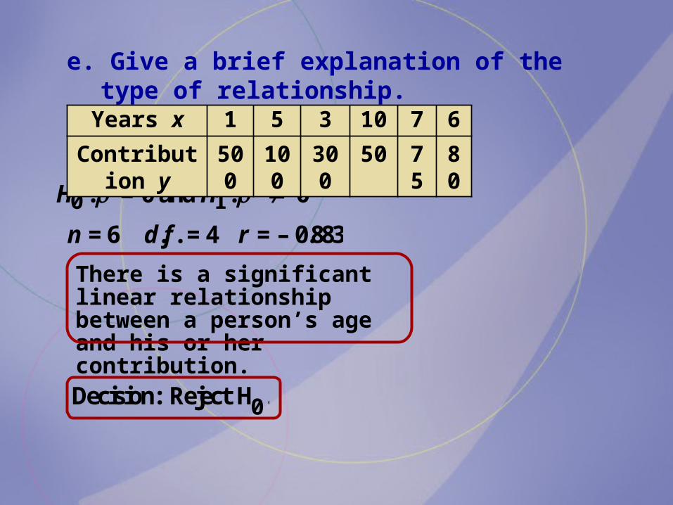
e. Give a brief explanation of the type of relationship.
0 1: = 0 and : 0H H
Years x 1 5 3 10 7 6
Contribution y 500 100 300 50 75 80
n = 6 d.f . = 4 r = – 0.883
There is a significant linear relationship between a person’s age and his or her contribution.
Decision: Reject H0 .

Section 10-3
Exercise #17
Chapter 10Correlation and Regression
For the following exercise, complete these steps.
a. Draw the scatter plot for the variables.
b. Compute the value of the correlation coefficient.
c. State the hypotheses.
d. Test the significance of the correlation coefficient at = 0.05, using Table I.
e. Give a brief explanation of the type of relationship.

A criminology student wishes to see if there is a relationship between the number of larceny crimes and the number of vandalism crimes on college campuses in Southwestern Pennsylvania. The data are shown. Is there a relationship between the two types of crimes?
Number of larceny crimes, x
24 6 16 64 10 25 35
Number of vandalism crimes y
21 3 6 15 21 61 20

a. Draw the scatter plot for the variables.Number of larceny
crimes, x24 6 16 64 10 25 35
Number of vandalism crimes y
21 3 6 15 21 61 20
20
4060
80
0 10 20 4030 50 60larceny crimes
vand
alis
m c
rimes
70 80

b. Compute the value of the correlation coefficient.Number of larceny
crimes, x24 6 16 64 10 25 35
Number of vandalism crimes y
21 3 6 15 21 61 20
y = 147
y2 = 5273
n = 7
x = 180
x 2 = 6914
xy = 4013
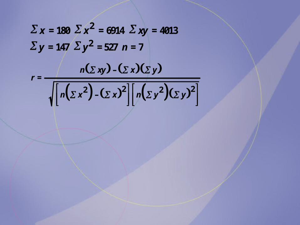
y = 147 y2 = 527 n = 7 x = 180 x 2 = 6914 xy = 4013
– =
2 22 2 –
n xy x yr
n x x n y y

y = 147 y2 = 527 n = 7 x = 180 x 2 = 6914 xy = 4013
4013 – 180 1476=
2 2 6 6914 – 180 5273 – 1476
r
r = 0.104
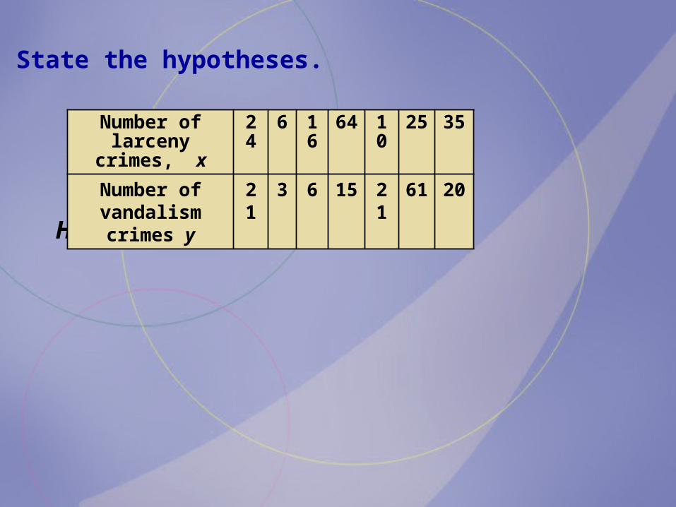
c. State the hypotheses.
0 1: = 0 and : 0H H
Number of larceny crimes, x
24 6 16 64 10 25 35
Number of vandalism crimes y
21 3 6 15 21 61 20

n = 7 d.f .= 5 r = 0.104
d. Test the significance of the correlation coefficient at = 0.05, using Table I.
Number of larceny crimes, x
24 6 16 64 10 25 35
Number of vandalism crimes y
21 3 6 15 21 61 20
C.V. = ± 0.754
Decision: Do not reject H0 .

e. Give a brief explanation of the type of relationship.
Number of larceny crimes, x
24 6 16 64 10 25 35
Number of vandalism crimes y
21 3 6 15 21 61 20
There is not a significant linear relationship between the number of larceny crimes and the number of vandalism crimes.
Decision: Do not reject H0 .
n = 7 d.f .= 5 r = 0.104

Section 10-3
Exercise #23
Chapter 10Correlation and Regression

a. Draw the scatter plot for the variables.
b. Compute the value of the correlation coefficient.
c. State the hypotheses.
d. Test the significance of the correlation coefficient at = 0.05, using Table I.
e. Give a brief explanation of the type of relationship.
For the following exercise, complete these steps.
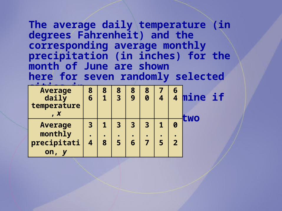
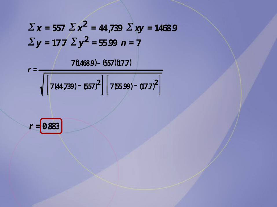
The average daily temperature (in degrees Fahrenheit) and the corresponding average monthly precipitation (in inches) for the month of June are shown here for seven randomly selected cities in the United States. Determine if there is a relationship between the two variables.
Average daily temperature, x
86 81 83 89 80 74 64
Average monthly precipitation, y
3.4 1.8 3.5 3.6 3.7 1.5 0.2

a. Draw the scatter plot for the variables.Average daily temperature, x
86 81 83 89 80 74 64
Average monthly precipitation, y
3.4 1.8 3.5 3.6 3.7 1.5 0.2
1
2
3
4
0 60Temperature
Prec
ipita
tion
70 80 90 100
5

b. Compute the value of the correlation coefficient.Average daily temperature, x
86 81 83 89 80 74 64
Average monthly precipitation, y
3.4 1.8 3.5 3.6 3.7 1.5 0.2
y = 17.7
y2 = 55.99
n = 7
x = 557
x 2 = 44,739
xy = 1468.9
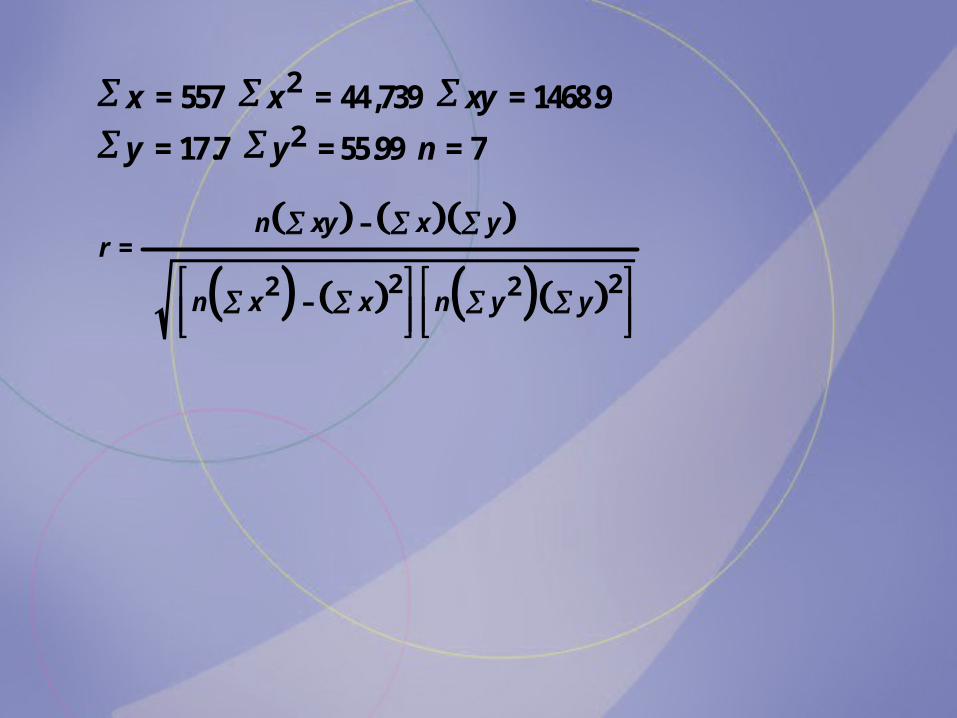
y = 17.7 y2 = 55.99 n = 7 x = 557 x 2 = 44,739 xy = 1468.9
– =
2 22 2 –
n xy x yr
n x x n y y
y = 17.7 y2 = 55.99 n = 7 x = 557 x 2 = 44,739 xy = 1468.9
r = 7(1468.9) – (557)(17.7)
7(44,739) – (557)2
7(55.99) – (17.7)2
r = 0.883

c. State the hypotheses.
Average daily temperature, x
86 81 83 89 80 74 64
Average monthly precipitation, y
3.4 1.8 3.5 3.6 3.7 1.5 0.2
0 1: = 0 and : 0H H

d. Test the significance of the correlation coefficient at = 0.05, using Table I.Average daily temperature, x
86 81 83 89 80 74 64
Average monthly precipitation, y
3.4 1.8 3.5 3.6 3.7 1.5 0.2
0 1: = 0 and : 0H H
C.V. = ± 0.754
Decision: Reject H0 .
n =7 d.f . = 5 r = 0.883
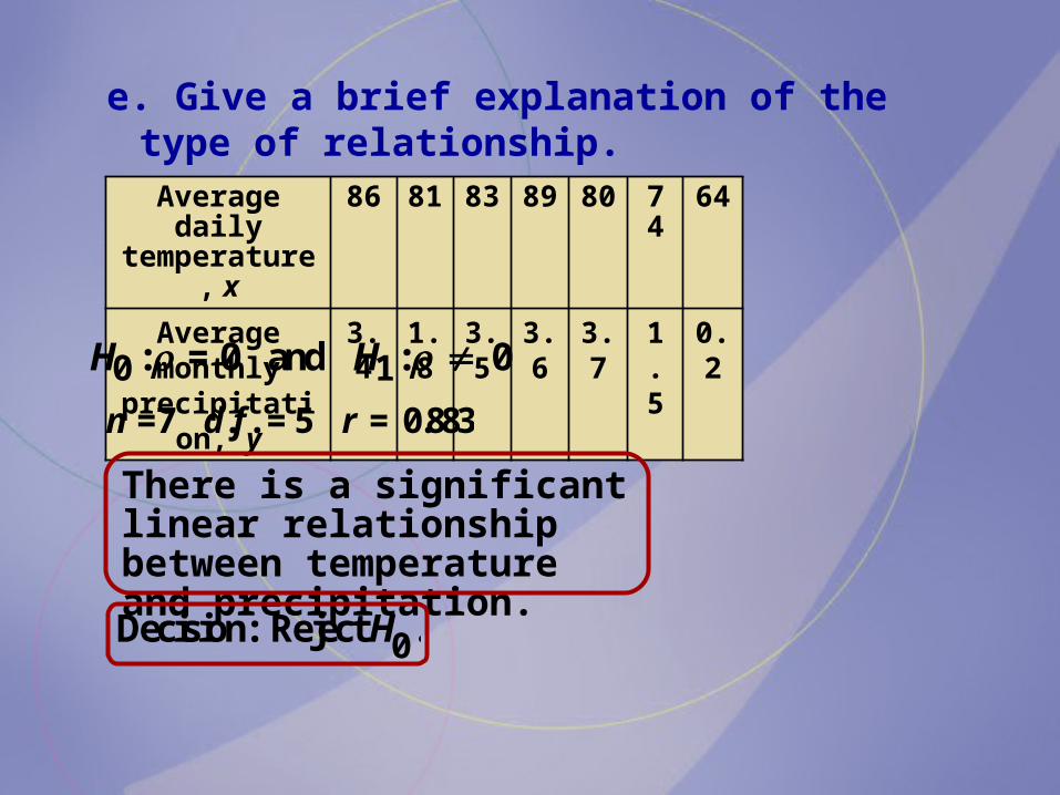
e. Give a brief explanation of the type of relationship.
Average daily temperature, x
86 81 83 89 80 74 64
Average monthly precipitation, y
3.4 1.8 3.5 3.6 3.7 1.5 0.2
0 1: = 0 and : 0H H
There is a significant linear relationship between temperature and precipitation.
Decision: Reject H0 .
n =7 d.f . = 5 r = 0.883
Chapter 10Correlation and Regression
Section 10-4Regression

Section 10-4
Exercise #13
Chapter 10Correlation and Regression

Find the equation of the regression line and find the y value for the specified x value. Remember that no regression should be done when r is not significant.
Ages and Exercise
11.532510Hours y
595238322618Age x

2
22
– =
–
y x x xya
n x x
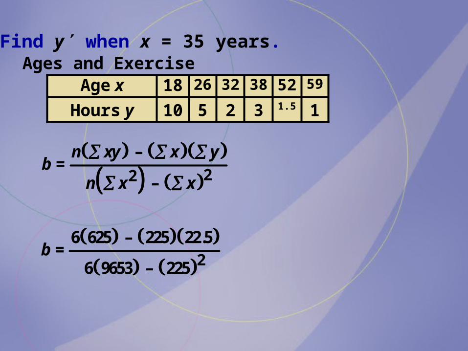
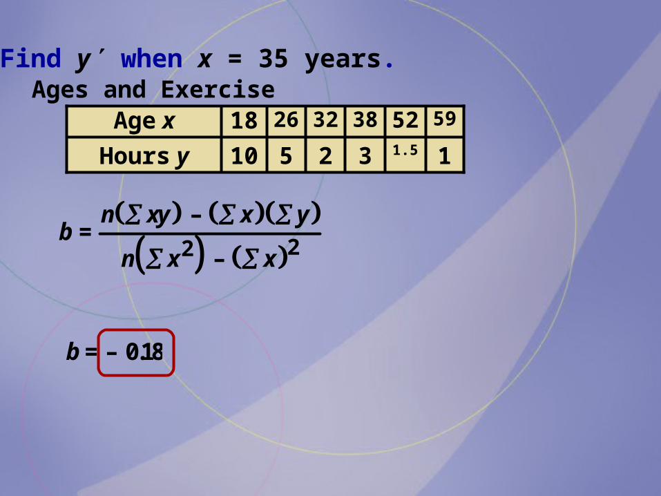
Find y when x = 35 years.Ages and Exercise
11.532510Hours y
595238322618Age x
2
22.5 9653 – 225 625 =
6 9653 – 225a

a = 10.499
2
22
– =
–
y x x xya
n x x
Find y when x = 35 years.Ages and Exercise
11.532510Hours y
595238322618Age x
Find y when x = 35 years.Ages and Exercise
11.532510Hours y
595238322618Age x
22
– =
–
n xy x yb
n x x
2
6 625 – 225 22.5 =
6 9653 – 225b
Find y when x = 35 years.Ages and Exercise
11.532510Hours y
595238322618Age x
22
– =
–
n xy x yb
n x x
b = – 0.18

Find y when x = 35 years.Ages and Exercise
11.532510Hours y
595238322618Age x
a = 10.499 b = – 0.18
y = a + bx
y = 10.499 – 0.18x
y = 10.499 – 0.18(35)
y = 4.199 hours

Section 10-4
Exercise #15
Chapter 10Correlation and Regression
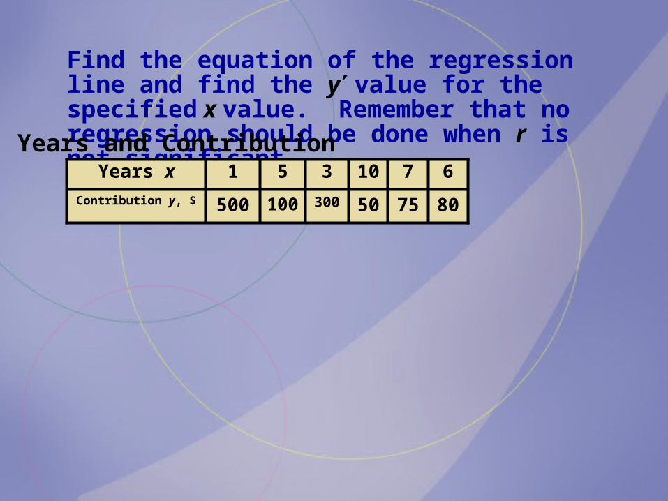
Find the equation of the regression line and find the y value for the specified x value. Remember that no regression should be done when r is not significant.Years and Contribution
807550300100500Contribution y, $
6710351Years x

2
22
– =
–
y x x xya
n x x
2
1105 220 – 32 3405 =
6 220 – 32a
Find y when x = 4 years.Years and Contribution
807550300100500Contribution y, $
6710351Years x

a =
243,100 – 108,9601320 – 1024
a = 134,140
296
2
1105 220 – 32 3405 =
6 220 – 32a
a = 453.176

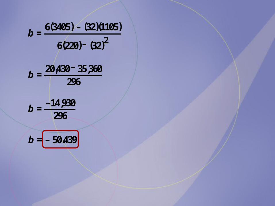
b = 6(3405) – (32)(1105)
6(220) – (32)2
22
– =
–
n xy x yb
n x x
Find y when x = 4 years.Years and Contribution
807550300100500Contribution y, $
6710351Years x
b = 6(3405) – (32)(1105)
6(220) – (32)2
b = – 50.439
b =
20,430 – 35,360296
b =
–14,930296

b = – 50.439
y = a + bx
y = 453.176 – 50.439x
y = $251.42
y = 453.176 – 50.439(4)
a = 453.176
Find y when x = 4 years.Years and Contribution
807550300100500Contribution y, $
6710351Years x

Section 10-4
Exercise #23
Chapter 10Correlation and Regression
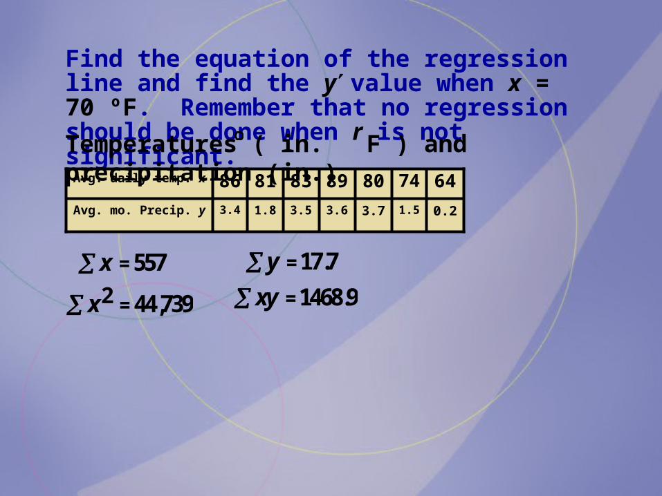
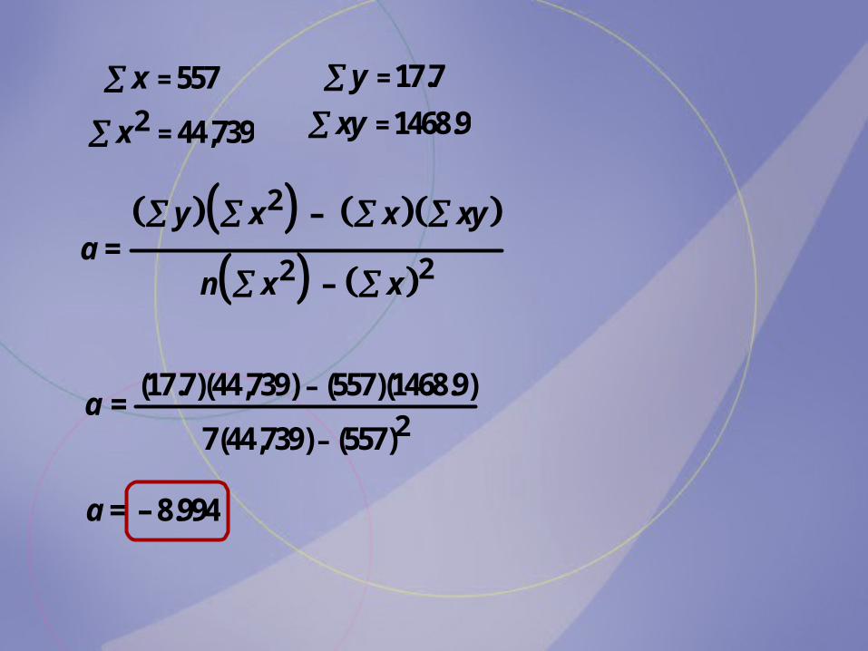
Find the equation of the regression line and find the y value when x = 70 ºF. Remember that no regression should be done when r is not significant.
0.2
64
1.53.73.63.51.83.4Avg. mo. Precip. y
748089838186Avg. daily temp. x
Temperatures ( in. F ) and precipitation (in.)
x = 557
x2 = 44,739
y = 17.7xy = 1468.9
x = 557
x2 = 44,739
y = 17.7xy = 1468.9
2
22
– =
–
y x x xya
n x x
a = (17.7)(44,739) – (557)(1468.9)
7(44,739) – (557)2
a = – 8.994

22
– =
–
n xy x yb
n x x
x = 557
x2 = 44,739
y = 17.7xy = 1468.9
b = 7(1468.9) – (557)(17.7)
7(44,739) – (557)2
b = 0.1448

y = a+ bx
y = – 8.994 + 0.1448x
y = 1.1 inches
y = – 8.994+ 0.1448(70)
a = – 8.994
b = 0.1448
x = 557
x2 = 44,739
y = 17.7xy = 1468.9

Chapter 10Correlation and Regression
Section 10-5Coefficient of Determination and Standard Error of the Estimate
Section 10-5
Exercise #9
Chapter 10Correlation and Regression
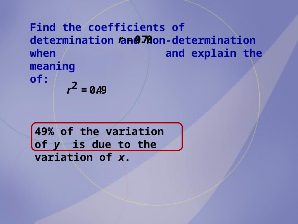
Find the coefficients of determination and non-determination when and explain the meaning of:
r2 = 0.49
r = 0.70
49% of the variation of y is due to the variation of x.

Find the coefficients of determination and non-determination when and explain the meaning of:
1– r 2 = 0.51
r = 0.70
51% of the variation of y is due to chance.

Section 10-5
Exercise #15
Chapter 10Correlation and Regression

Compute the standard error of the estimate.
x = 225
x2
= 9653
xy = 625
y = 22.5
y2 = 141.25
n = 6
a = 10.499 b = – 0.18
sest =
y 2 – a y – b xy
n – 2
s
est=
141.25 – 10.499(22.5) – (– 0.18)(625)
6 – 2

sest =
141.25 – 10.499(22.5) – (– 0.18)(625)
6 2
sest = 4.380625
sest = 2.09

Section 10-5
Exercise #19
Chapter 10Correlation and Regression

Find the 90% prediction interval when x = 20 years.
x = 225
y = 22.5
x2
= 9653
y2 = 141.25
xy = 625
n = 6
a = 10.499
b = – 0.18
Age x 18 26 32 38 52 59
Hours y 10 5 2 3 1.5 1
y = 10.499 – 0.18x
= 10.499– 0.18(20) = 6.899

x = 225
y = 22.5
x2
= 9653
y2 = 141.25
xy = 625
n = 6
a = 10.499
b = – 0.18
y = 6.899
2
2 2( )11 + +
( )– < 2
n x Xyy t s nest n x x
2
2 2– + +
( )1< + 1 2( )
n x Xy t sest n n x x
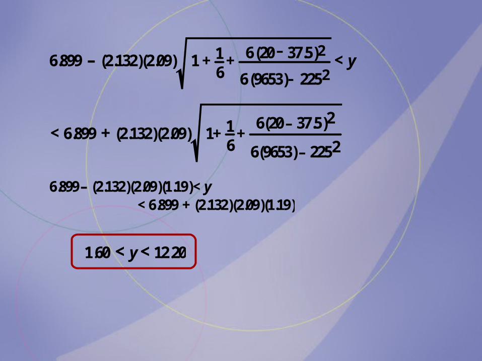
1.60 < y < 12.20
6.899 – (2.132)(2.09) 1 + 16
+ 6(20 – 37.5)2
6(9653) 2252< y
< 6.899 + (2.132)(2.09) 1+ 16
+ 6(20 – 37.5)2
6(9653) – 2252
6.899– (2.132)(2.09)(1.19)< y
< 6.899 + (2.132)(2.09)(1.19)

Section 10-5
Exercise #21
Chapter 10Correlation and Regression

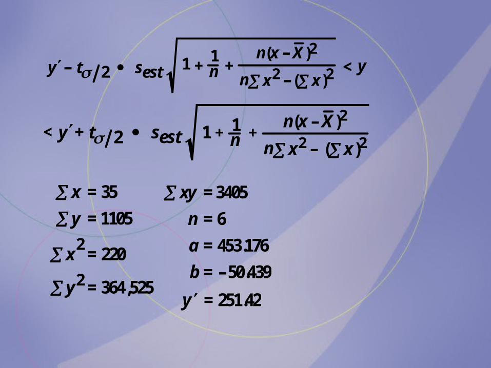
Find the 90% prediction interval when x = 4 years.
Years x 1 5 3 10 7 6
Contributions y, $ 500 100 300 50 75 80
x = 35
y = 1105
x2
= 220
y2 = 364,525
xy = 3405
n = 6
a = 453.176
b = – 50.439
y = 453.176 – 50.439x
= 251.42 = 453.176 – 50.439(4)
2
2 2( )11 + + 2 ( )
–– <
–
n x Xyy t s nest n x x
2
2 2 + +
( – )1< + 1 2– ( )
n x Xy t sest n n x x
x = 35
y = 1105
x2
= 220
y2 = 364,525
xy = 3405
n = 6
a = 453.176
b = – 50.439
y = 251.42

$30.46 < y < $472.38
251.42 – (2.132)(94.22) 1 + 16
+ 6(4 – 5.33)2
6(220) – 322< y
< 251.42+ (2.132)(94.22) 1 + 16
+ 6(4 – 5.33)2
6(220) – 322
251.42 – (2.132)(94.22)(1.1) < y
< 251.42+ (2.132)(94.22)(1.1)

Chapter 10Correlation and Regression
Section 10-6Multiple Regression

Section 10-6
Exercise #7
Chapter 10Correlation and Regression
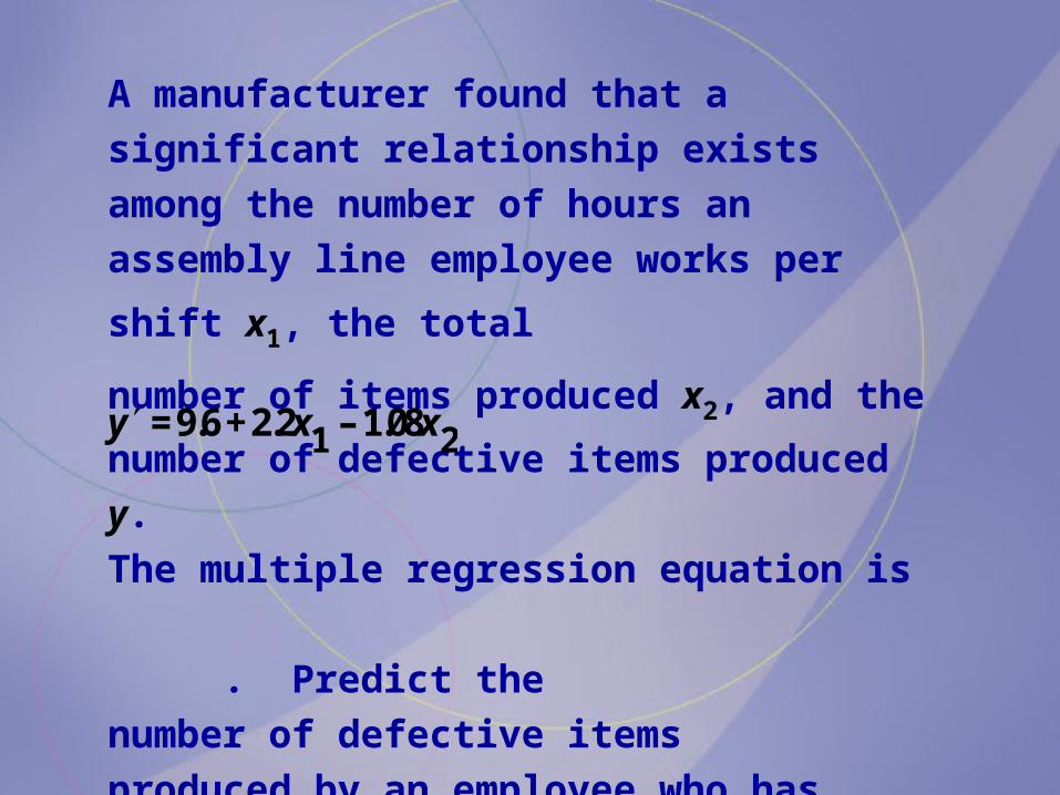
A manufacturer found that a significant relationship
exists among the number of hours an assembly line
employee works per shift x1, the total
number of items produced x2, and the
number of defective items produced y.
The multiple regression equation is
. Predict the
number of defective items
produced by an employee who has
worked 9 hours and produced
24 items.
y = 9.6 + 2.2x1 – 1.08x2

y = 3.48 or 3 items
y = 9.6 + 2.2x1 – 1.08x2
= 9.6 + 2.2 9 – 1.08 24y

Section 10-6
Exercise #9
Chapter 10Correlation and Regression

An educator has found a significant relationship among a college graduate’s IQ x1, score on the verbal section
of the SAT x2, and income for the first year
following graduation from college y. Predict the income of a college graduate whose IQ is 120 and verbal SAT score is650. The regression equation is
y ' = 5000 + 97x1+ 35x2 .
y = 5000+ 97(120) – 35(650)
y = $39,390


