6−3−1

Section 6-3 Computation of Mean Areal Precipitation Introduction Good estimates of precipitation are critical to the successful use of conceptual models. The precipitation estimates should first of all conform to the physical scale of what actually occurs in nature, i.e. the estimates should be unbiased compared to what actually occurs. Second, other statistical properties of the estimates, such as frequency of occurrence of various amounts and seasonal variability, should also be as realistic as possible. Third, the amount of random error in the estimates should be as small as possible. The random error is controlled to a large degree by the data network and spatial variability of precipitation over the region. In sections of the country where there is a high spatial correlation between precipitation amounts the typical climatological network can produce a fairly reliable areal estimates, whereas in areas with little spatial correlation the estimates will contain a large amount of random error. A large amount of noise in the precipitation input makes it very difficult to determine model parameters and obtain good simulation results. The quality of the areal precipitation estimates largely determines where lumped, conceptual models can be applied with satisfactory results (see Figure 1-1 in chapter 1). Prior to doing the steps discussed in this section it is assumed that all the precipitation data are available in the proper form and that the data have been checked for consistency and adjusted if necessary. It is also assumed that the areas where MAP estimates are to be generated have been determined based on the definition of the flow points needed for calibration and the possible subdivision of the drainage areas into elevation zones or subareas specified by other means. It is also assumed that it has been determined as to whether mountainous or non-mountainous area procedures should be used to compute areal estimates. Ideally precipitation data should be corrected for gage catch deficiencies prior to computing areal estimates for use in conceptual models. Catch deficiencies are a function of the type of precipitation, the type of gage, and the amount of wind at the orifice of the gage. The catch deficiencies for snow are much greater than for rain. The wind speed at the gage orifice is controlled by the current atmospheric wind speed and direction, the gage exposure, and the type of wind shield, if any. The catch deficiency varies throughout an event as meteorological conditions change. Some techniques have been proposed for applying monthly adjustments to precipitation data at a given station based on wind and temperature data from nearby synoptic sites and a general classification of the gage exposure including whether a wind shield is installed. Whether the application of such techniques would improve model simulation results has not be shown. In non-mountainous areas gage catch deficiencies are typically ignored when computing MAP. An average catch deficiency for snow events is later incorporated in the snow model computations (e.g. the SCF parameter in the SNOW-17 model). In mountainous areas some adjustment for the average catch deficiency can be implicitly included when water balance computations are used to obtain average areal precipitation estimates. Further adjustment is likely when the models are calibrated (see discussions under the SCF parameter in sections

6−3−2

7-4 and 7-7). Time Interval for Precipitation Computations The Mean Areal Precipitation (MAP) processing program in NWSRFS used for calibration will allow for the generation of time series at a 1,3, and 6 hour interval. In most cases a 6 hour interval should be used. There are several reasons for using a 6 hour time interval when generating MAP time series from historical raingage data. First, the program used operationally in NWSRFS to generate MAP time series from raingage reports currently will only generate time series at a 6 hour time interval. Second, in most regions there is not a dense enough historical hourly raingage network to produce reliable areal estimates at less than a 6 hour interval. Third, since some of the models, especially the Sacramento Model, will produce different results depending on the time scale that they are applied, the calibration of the model and the operational application should use the same time interval. Historically for river forecasting at an RFC a 6 hour time interval has been used for model computations. This has typically been the case for several reasons. First, real time data, especially precipitation, was only available on a 6 hour basis at a reasonable network density. Second, the time needed operationally to obtain and process data, perform model computations and make manual adjustments, and get the forecasts to the users limited the time between forecast updates to around 6 hours. Third, RFCs were not opened on a 24 hour basis except during times of significant flooding potential. Thus, when the current OFS MAP program was coded in the 1980's a 6 hour time interval was specified. The use of a 6 hour computational interval has also tended to limit the size of the basins that are modeled by the RFCs to those that can be modeled successfully at a 6 hour interval, i.e. basins that typically peak in 12 or more hours. Drainages with faster response times have been handled using site specific and regional flash flood procedures by the WFO or via local flood warning systems such as ALERT and IFLOWS. The WFO and local flood warning procedures seldom involve continuous modeling and rely on previously prepared guidance material. With the automation of more data networks, there now are considerable data available operationally at intervals of 1 hour or less in some parts of the United States, however, the availability of hourly data from the climatological network is still limited and the OFS MAP program still produces time series at only a 6 hour interval. Techniques are now available in OFS to use gridded hourly precipitation estimates generated by merging radar, raingage, and other data, however, studies have shown that these estimates in most cases are biased as compared to MAP values generated from historical raingage data. There is of course also the scale effects of the models which must be accounted for prior to using hourly precipitation estimates operationally with models that are calibrated at a 6 hour time interval. A further discussion of historical versus operational bias and scale effects is included in chapter 8 of this manual. If there are sufficient historical hourly stations, a 1 or 3 hour MAP time series could be generated and used for calibration. If snow is also a factor, the SNOW-17 model allows for the generation of the rain plus melt time series at the same interval as the precipitation time series even if te

6−3−3

mperature data are only at a multiple of the precipitation data time interval. Thus, for example, SNOW-17 will produce hourly rain plus melt from hourly MAP data and 6 hour temperature estimates (the NWSRFS historical temperature processing program only produces 6 hour mean areal estimates). In order to then use such calibration results for operational forecasting would require a procedure that would produce real time hourly estimates of precipitation from raingage data or the assurance that there was no bias between the historical MAP values and hourly radar based estimates available operationally. Non-Mountainous Area Precipitation Estimates Introduction Even though it has been previously decided by looking at the station data and other factors that the non-mountainous area procedure can be used to generate MAP estimates, it is probably a good idea to reexamine the station data after the consistency checks and adjustments have been completed to make sure that the variation in average station precipitation over the river basin conforms to the definition of a non-mountainous area. If so, the computation of the MAP time series is quite straight forward. Background The MAP program of NWSRFS uses the following sequence when completing the data record by estimating all missing data values and time distributing accumulated amounts.

1. Estimate all missing hourly station values using only other hourly stations since these are the only data that always correspond exactly to the time period of the missing record. Also time distribute any accumulated amounts at hourly stations based on the other stations in the hourly data network. If there are no estimator stations available for certain periods, i.e. all hourly stations have missing data, then the estimates are set to zero for all the hourly stations for these periods. The program lists the number of hours that this occurs. If the number of hours that precipitation is set to zero is significant (something like more than 0.1% of the period of record), more hourly stations should be added to the analysis if possible. This is most important when some of the hourly stations are assigned weight for computing MAP values. 2. Time distribute all observed values at daily reporting stations into hourly estimates based on the observation time of the daily report and the stations in the hourly network. If no hourly data are available to time distribute a daily value, i.e. all hourly stations were missing or recorded no precipitation, the daily total is currently assigned to the hour of the observation time and the other hours in the day are set to zero. The program tabulates the number of days for each station when the daily total can’t be distributed for amounts greater and less than 0.5 inches. The maximum daily amount that couldn’t be distributed is also tabulated for each station. If the number of cases for some stations are much larger than for the majority, this may indicate a problem with the observation times specified for those stations. Such discrepancies can also occur for daily stations that are not in the vicinity of any hourly stations or for

6−3−4

high elevation daily reporting stations when all the closest hourly stations are at much lower elevations. Correcting the observation time histories and adding additional hourly stations, if available, are the only ways to reduce the number of days when the distribution of daily amounts is not possible. However, even in the best of cases there will always be many days when isolated storms effect only daily stations. 3. Estimate the missing values at daily reporting stations based on the observation time of the report and all available hourly estimates from both the hourly network and daily stations that were time distributed in step 2. The missing daily totals are then time distributed into hourly amounts just like the observed daily data.

After this process is complete, all of the stations have a complete record, i.e. no missing or accumulated data, and the data for each station are defined at an hourly time interval. Station weights can then be multiplied times the data values and the results summed up over the specified time interval to generate the MAP time series for each subarea. The equation used for estimating missing precipitation data in non-mountainous areas is:

(6-3-1) where: P = precipitation amount x = station being estimated i = estimator station n = number of estimator stations, and d = distance The estimator stations are the closest stations with available data in each quadrant surrounding the station being estimated. The quadrants are based on the roughly 4 km HRAP grid system. Estimated amounts are not used to estimate other amounts. The same weights, i.e. 1/d2, are also used to time distribute accumulated amounts. Equation 6-3-1 assumes that the mean precipitation at all the estimator stations can be assumed to be the same as the station being estimated, which is the basic assumption of the non-mountainous area procedure. Station Weights The assumption for a non-mountainous area is that the mean precipitation is essentially the same at all locations with the basin, not only where there are stations, but also at all points in between. Thus, station weights can be determined merely by the location of the gages within the boundaries of the area. This requires that basin boundaries, i.e. latitude, longitude points that define th

6−3−5

e outline of the basin, are available. There are two methods in the MAP program for calculating station weights using gage and boundary locations, Thiessen weights and grid point weights. Both are generated within the program by overlaying the HRAP grid over the area. For Thiessen weights, the weight for each HRAP grid point is assigned to the closest station. For the grid point method, the weight for each grid point is divided based on the 1/d2 technique to the closest station in each quadrant. For both methods, the weight assigned to each station from all grid points is then summed and normalized to obtain the station weights. These weights will always sum to 1.0. Both methods produce fairly similar weights, though the grid point method assigns some weight to stations outside the boundaries that will not receive any weight with the Thiessen method. The Thiessen method is the preferred way to compute station weights in most cases. Mountainous Area Precipitation Estimates Introduction As discussed earlier, in a mountainous area the mean precipitation is spatially variable. Thus, the estimation of missing data must account for the fact that the precipitation catch at the estimator stations may be different than at the station being estimated. Also, station weights cannot be computed based on the location of the gages with the boundaries of the area. The procedure outlined in this section was primarily developed to make it relatively easy to minimize bias between historical (calibration) estimates of MAP and subsequent operational estimates. For model parameters determined during calibration to perform in a similar manner during operational use, it is imperative that there is not a bias between the precipitation values used as input to the two applications of the model. The procedure relies heavily on isohyetal analyses of long-term precipitation patterns. Good isohyetal maps are essential to the success of the method. By using an isohyetal analysis as the basis for computing areal estimates, the typical precipitation pattern defined by the isohyetal maps is used to interpolate between station values and used to extrapolate into ungaged portions of the area. In many mountainous watersheds there are no stations at the highest elevations, thus the relationships defined by the isohyetal maps are used to estimate the amount of precipitation falling above the highest gages. This works well over the long term, but can result in errors for individual storms due to changing dynamics from one storm to the next. Since model parameters are based on the simulation of many events, these random errors for individual events should not affect the determination of parameter values during calibration. Operationally it would be beneficial to have a procedure that would account for the changing storm dynamics and still maintain the same long term pattern defined by the isohyetal maps used during calibration. The suggested steps for computing MAP in mountainous areas is as follows:

1. Determine mean monthly precipitation for each station for the period of record, 2. Determine if station weighting should be done on an annual or seasonal basis, 3. Determine the mean seasonal or annual precipitation for the historical data period for each area within the river basin where MAP time series are to be generated after checking the isoh

6−3−6

yetal maps to determine if adjustments are needed for incompatibilities in the periods of record, differences between station data and isohyetal map estimates, or disparities based on a water balance analysis, 4. Determine annual or seasonal station weights for each MAP area by adjusting subjectively determined relative weights so that the correct areal average precipitation for the historical period of record will be generated, and 5. Compute MAP time series for each area within the river basin for the period of record using the predetermined station weights determined in step 4.

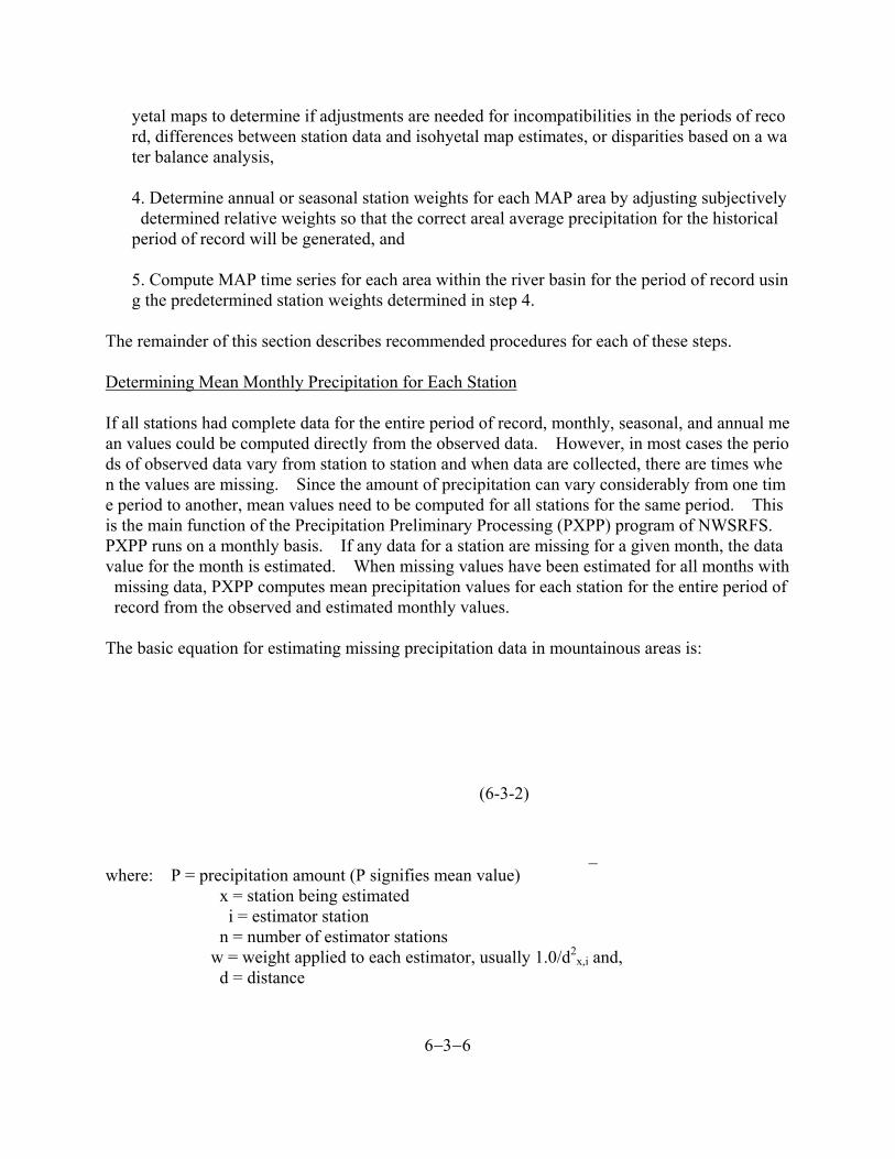
The remainder of this section describes recommended procedures for each of these steps. Determining Mean Monthly Precipitation for Each Station If all stations had complete data for the entire period of record, monthly, seasonal, and annual mean values could be computed directly from the observed data. However, in most cases the periods of observed data vary from station to station and when data are collected, there are times when the values are missing. Since the amount of precipitation can vary considerably from one time period to another, mean values need to be computed for all stations for the same period. This is the main function of the Precipitation Preliminary Processing (PXPP) program of NWSRFS. PXPP runs on a monthly basis. If any data for a station are missing for a given month, the data value for the month is estimated. When missing values have been estimated for all months with missing data, PXPP computes mean precipitation values for each station for the entire period of record from the observed and estimated monthly values. The basic equation for estimating missing precipitation data in mountainous areas is:

(6-3-2) _ where: P = precipitation amount (P signifies mean value) x = station being estimated i = estimator station n = number of estimator stations w = weight applied to each estimator, usually 1.0/d2

x,i and, d = distance

6−3−7

PXPP solves this equation by establishing a base station and then computing the ratio of precipitation at each station to that caught by the base station for each month of the year. The base station must be a station with very little missing data during the period of record and should be a station that is naturally consistent (i.e. consistency corrections are not needed). A station with a low catch, as compared to the other stations, should not be used as the base station. The base station should be one with a moderate to high catch to avoid very high ratios being computed during months with little or no precipitation. The location of the base station within the region being used in the analysis is not critical. The ratio of precipitation at a given station to that caught at the base station for each month is computed using all years for which both stations have complete data for the month. If both stations have overlapping data for about 5 or more years, a fairly stable relationship can be determined. PXPP then substitutes the ratio to base for the appropriate month for station x and station i in place of the mean precipitation values into Eq. 6-3-2 in order to determine the average ratio of station x to station i. In this way Eq. 6-3-2 is used to compute precipitation for months with missing data. Reasonable estimates of mean monthly precipitation cannot be computed by PXPP for stations with little or no overlapping data with the base station. Since the base station is usually selected partly because it has data for essentially the entire period of record, these are usually stations with very short records or with frequent missing data such that monthly totals seldom can be calculated. Typically such stations are not adding much information to the precipitation analysis and thus would be discarded. The only other option is to remove such stations from the PXPP runs and then estimate their mean monthly values based on other stations and monthly averages derived from the isohyetal maps so that they can be included in the MAP program. Within the PXPP program, determining mean values over the period of record and making consistency checks and corrections is an iterative process. Consistency corrections will increase or decrease the observed values for some portion of the period of record and thus change not only the computed mean values for the station being corrected, but also the mean values for stations using the corrected data to estimate missing months. After consistency corrections and mean monthly values (referred to as characteristics in some cases) have been computed using PXPP, the MAP program should be run to verify that the consistency plots are similar between the two programs. Typically the plots look basically the same, but sometimes the plots are slightly different for one or two of the stations, generally hourly stations, due to differences in the computational sequence in the two programs. In MAP, as mentioned in the non-mountainous area section of this section, hourly stations can only be estimated from other hourly stations, whereas in PXPP each station can be estimated from all the others. If inconsistencies show up in MAP that were not present in the final PXPP run, these can sometimes be removed by changing or adding consistency corrections to the affected stations in the MAP run. Changing consistency corrections in the MAP program will not automatically change the mean monthly values (characteristics) being used by the program (adjustments to the mean monthly values could be made by the user if the change in the consistency correction is significant). In Alaska there is very little hourly precipitation data available from the NCDC climatological ne

6−3−8

twork. In fact only a handful of stations are available over the entire state and most of these have a short period of record. Even those with the longest record, Anchorage and Fairbanks, don’t go back to when many of the daily digital records began in water year 1949. Some hourly data can be obtained from real time stations for use in the historical analysis, but these are generally very short records and many of the sites have considerable missing data. The result is that only a few of the hourly stations have sufficient data for use in PXPP and in many cases these gages are located far from the river basin being processed. However, the MAP program requires that hourly stations be available. One solution to this problem is to remove any hourly stations that don’t have sufficient data overlapping with that of the base station from the PXPP runs. Then estimate the mean monthly values for these stations based on nearby stations and the isohyetal maps so that they can be included in the MAP program. However, rather than locating the stations at their actual location which can cause problems when estimating missing data, position the stations at locations surrounding, but far outside, the other stations being used for the river basin. These hourly stations will then be used for time distribution of daily amounts whenever they have observed data, but their 1/d2 values will be very small and will not affect the estimation of missing data for the daily stations being used. Annual versus Seasonal Station Weights The MAP program allows for station weights (predetermined) in mountainous areas to be specified on an annual or seasonal basis. Seasonal weights are beneficial in regions where the spatial pattern of precipitation is greatly different in one season than in another. This is typically caused by different types of storms predominating at different times of the year. The region where seasonal weights are typically needed is the intermountain west. In this region large scale storms with significant orographic effects dominate during the winter, while small scale convective events cause most of the summer precipitation. In most other regions of the United States the precipitation patterns do not vary sufficiently enough from one season to the other to justify the use of seasonal weights. In these regions annual weights are generally fully adequate. Since the MAP program allows for only a single definition of the winter and summer seasons, the seasons used for station weighting and for consistency checks must be the same. In most cases, especially in the intermountain west, the seasons to use for these two features are the same for all practical purposes so this doesn’t present a problem. There are two types of plots that can be constructed to help in deciding whether seasonal station weights need to be used. The first, is to plot the seasonal relationship between a high elevation station and a nearby low elevation station. Ideally the two stations selected should have the same orographic exposure, i.e. both on the same side of a major divide and not one on the windward side and the other on the leeward side. This high-low precipitation plot is generated by plotting the monthly ratio of the average catch based on the PXPP program results at the two stations. If the monthly ratio of precipitation from the two stations is quite similar throughout the year, there is little benefit to be gained by using seasonal station weights, whereas if there is a significant variation and a distinct seasonal pattern in the ratio, then seasonal weights should be used.

6−3−9

Figure 6-3-1. High-low precipitation plots for locations in the intermountain west and New England. (The Big Timber watershed plot is based on the Monument Peak SNOTEL site at 8850 feet and the Big Timber climatological station at 4100 feet. The White Mountain plot is based on climatological stations at Mount Washington (elev. 6262 feet) and Bretton Woods (elev. 1621 feet).)

6−3−10

Figure 6-3-1 shows such plots for two gages within the Big Timber watershed just north of Yellowstone National Park in Montana and for two gages in the White Mountains of New Hampshire. In the Big Timber case there is a very large difference in ratios from mid-winter when large orographic storms dominate to mid-summer when most of the precipitation is produced by small scale convective events. Seasonal weights are certainly justified in this region. The typical winter season in the intermountain west is from October to April and the summer season from May to September. Based on the Big Timber plot a winter season from November through March might be better for station weights, though the October to April season is probably more appropriate as far as when snowfall predominates for making consistency adjustments. For the White Mountains annual station weights can be used since the variation in the high-low precipitation ratio is similar throughout the year. The idea for using plots of high elevation to low elevation precipitation stations to get an insight into seasonal changes in precipitation patterns was introduced by Eugene Peck, former Director of the NWS Hydrologic Research Laboratory, [1964]. By examining pairs of high and low elevation stations scattered throughout the western mountains he showed that there were significant seasonal variations over much of the intermountain west, but little seasonal change in the ratios west of the Pacific Crest.

The second type of plot that is helpful in deciding whether to use seasonal station weights is a plot of precipitation versus elevation for each season. If the plots for the two seasons are dissimilar, this would indicate that the types of storms producing the precipitation are different and thus, seasonal station weighting would be appropriate, whereas if the relationship between precipitation and elevation is similar throughout the year, annual station weighting is sufficient. The high - low plot is best for defining the seasons to use for station weighting, but it only shows the relati

6−3−11

onship between two stations in the basin. The precipitation versus elevation plots are used to confirm whether the precipitation patterns are different for the entire network. Figure 6-3-2 shows precipitation versus elevation plots for an area in the upper Yellowstone River basin.

Figure 6-3-2. Precipitation versus elevation plots for the Upper Yellowstone River basin in Montana and Wyoming. Winter season is October through April, summer season is May through September.

This plot shows much more variation in precipitation with elevation, especially at the higher elevations, in the winter season than during the summer, i.e. the orographic effects are much larger during the winter months. This clearly suggests that seasonal station weighting would be appropriate. Such differences in the precipitation versus elevation relationships are common throughout the intermountain west. Determination of Average Mean Areal Precipitation for Each MAP Area The next step for computing MAP in mountainous areas is to determine the average mean areal precipitation on a seasonal or annual basis for the historical period of record for each of the MAP areas within the river basin. This is done by averaging the precipitation shown on the isohyetal maps over each of the MAP areas either on an annual or seasonal basis and then applying any necessary adjustments to the result. Adjustments can be needed for several reasons. First, if the period used to produce the isohyetal map differs from the period of historical record being used, an adjustment may be needed. Second, the mean precipitation values determined for the stations being used to compute the MAP time series should be compared against the estimate for these sites from the isohyetal maps to determine if adjustments are needed to portions of the isohyetal analysis and whether the station data makes sense. Third, water balance computatio

6−3−12

ns need to be made to determine if runoff information suggests adjustments to the areal mean derived from the isohyetal maps. The first check to perform is whether the periods of record used to produce the isohyetal maps are the same as the period of record being used for the historical analysis. It is most likely that they are not the same. In that case, one needs to determine if adjustments need to be applied to the isohyetal analysis so that it reflects the historical period. The most straight forward way to do this is to take a number of the stations with long data records and compute the ratio of the average annual precipitation over the historical data period to the same value for the isohyetal map period of record. The average station precipitation determined by the PXPP program would be used to compute these ratios. If these ratios differ significantly from 1.0, then an adjustment is needed. If the ratios for all stations are fairly similar in magnitude, then the average ratio can be used to adjust the isohyetal maps. If there is a pattern to the ratios over the river basin, a different adjustment could be used for different parts of the basin. While annual precipitation should be sufficient for computing this adjustment, one could compare seasonal ratios if the MAP analysis was being done on a seasonal basis to confirm if the adjustment is similar for each season. The second check is to compare the mean values for the stations being used for calibration as determined by the PXPP program with the mean values for these sites from the isohyetal analysis (any period of record adjustment determined in the first check should be applied to the station values picked off the isohyetal maps). This should be done on a seasonal basis for those river basins where it has been determined that seasonal station weights are appropriate for computing MAP. While the isohyetal analyses have generally been done in a careful manner with proven techniques, the results cannot be treated as the ‘true’ definition of what actually occurred. The data being used for calibration are typically more complete than the data used to generate the isohyetal maps. Generally the isohyetal maps use only stations with a long period of record, whereas in calibration we also use stations with shorter records to better define the spatial variability. Also all the calibration stations should have been checked for consistency and adjusted if needed, whereas, this is probably not the case for all the stations used to generate the isohyetal maps. The best way to visualize differences between the station data and the isohyetal analysis is to plot the ratio of the value picked off the isohyetal map at each station location divided by the PXPP value for the station on a map of the river basin. Ideally the ratios should vary around 1.0. Isolated values that differ significantly from 1.0 could represent a small scale problem with the isohyetal analysis or could indicate a problem with the data for that station. If there are portions of the river basin where the ratios are quite different from 1.0 and exhibit a definite pattern, this most likely indicates that the isohyetal maps are over or under estimating the amount of precipitation in these areas; thus the long-term average values for the affected MAP areas derived from the isohyetal analysis will need to be adjusted. Before making any corrections it is best to do a water balance analysis to confirm that adjustments are needed for watersheds in these portions of the river basin. Most isohyetal analyses are done using only station precipitation data. The techniques being used then interpolate and extrapolate these station data using elevation, aspect, prevailing storm direction, and other factors to estimate the average precipitation pattern over the region being studie

6−3−13

d. One way to determine if the average volume of precipitation shown on an isohyetal map is realistic is to do a water balance analysis. The water balance equation for a watershed can be expressed as:

P - R - ΔS - L = ET (6-3-3) where: P = average annual precipitation, R = average annual runoff, ΔS = average annual change in storage, L = average annual losses or gains due to transfers across watershed boundaries or losses to deep groundwater aquifers, and ET = average annual evapotranspiration.

Over a sufficiently long period the change in storage term should be essentially zero except for watersheds with a significant glaciated area. The watersheds used for a water balance analysis would be headwater areas with a value of the L term equal to zero and few complications such as large reservoirs or substantial irrigated acreage. Local areas could also be included as long as the area is relatively large enough so that a reliable estimate of the local runoff can be determined by subtracting upstream flows from downstream flows. The precipitation used would be that derived from the isohyetal analysis adjusted to the historical period of record. The runoff would be the mean annual runoff for this same period. In many cases the period of record of the streamflow data used to compute average annual runoff is less than the period of record being used for historical data analysis. For these watersheds MAP time series should be generated for all subareas using the mean areal average computed directly from the isohyetal analysis (adjusted for calibration period of record). Then the average annual precipitation for use in the water balance computation can be calculated for the same years as the runoff data. In these cases, which is typical for many watersheds, one would complete the remaining steps in the MAP computational procedure so that time series would be available to determine the proper annual precipitation to use in the water balance equation and then if further isohyetal map adjustments were needed, the steps would be repeated using adjusted values of the mean areal averages. The average annual ET determined from the water balance computations for as many watersheds as possible over the river basin should be tabulated for comparison. Another good way to see if the computed ET values make sense is to plot them against elevation. The variation in ET over the basin and with elevation should make sense. If there are watersheds that deviate significantly from a reasonable variation of ET over the basin, it is likely that the isohyetal map needs to be adjusted for these areas. If these watersheds correspond to the portions of the basin where the ratio of the station data to the isohyetal map estimate for the station were substantially different from 1.0, this further indicates that there are problems with the isohyetal estimates of precipitation over those areas. Adjustments should then be determined so that a more reasonable estimate of the average mean areal precipitation, annual or seasonal, can be used for computing each of the MAP time series. For watersheds included in the water balance analysis, the adjustments are based on both the water balance and patterns in the plots of the ratios of observed station data to

6−3−14

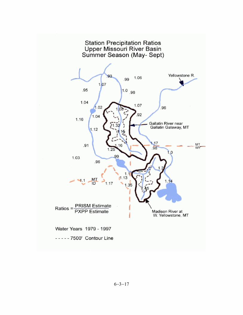
the isohyetal estimates. For other drainages in the river basin, the adjustments are based on the patterns shown in the ratio plots. Water balance computations in regions with large glaciated areas is more complex. In these cases, one needs to have a general idea as to whether there was a significant gain or loss of ice stored in the glaciers over the period being analyzed. Then either an attempt can be made to estimate the ΔS term in Eq. 6-3-3 so that ET variations could be computed directly or the value of ET + ΔS can be computed. Then ideally one could compare the ET + ΔS values for watersheds with and without glaciers, or at least with different amounts of glacial coverage, to see if the variation makes sense. To illustrate these last two checks, we will look at a portion of the Upper Missouri River basin near Yellowstone National Park. Figures 6-3-3 and 6-3-4 show plots for both the winter and summer seasons of the ratio of the estimate picked off the isohyetal maps at each station location divided by the PXPP precipitation estimate for each station. For illustration purposes two watersheds, as well as their two elevation zones, are outlined on these plots; the Gallatin River near Gallatin Gateway, Montana and the Madison River near West Yellowstone, Montana. While the ratios tend to scatter around 1.0 over much of this region, there are definite places where there is a pattern of values greater than 1.0. Ratios greater than 1.0 appear over the drainage area of both of the outlined watersheds suggesting that the PRISM precipitation estimate is likely too large. Table 6-3-1 shows the results of water balance computations for a number of watersheds in this region. The ET values from Table 6-3-1 are plotted against the the mean elevation of each watershed in Figure 6-3-5. This plot shows a reasonable variation in ET versus elevation for most of the watersheds, however, the values for the Gallatin and

6−3−15

6−3−16

Figure 6-3-3. Winter season precipitation ratios for the Upper Missouri River basin.

6−3−17

6−3−18

Figure 6-3-4. Summer season precipitation ratios for the Upper Missouri River basin.

6−3−19

Watershed

Period

Elevation

Pcpn

Runoff

ET

Stillwater R. nr. Absarokee,MT

wy 79-95

7186.

29.5

12.2

17.3

Clark Fk. nr. Belfry, MT

wy 79-97

7463.

27.7

9.5

18.2

Big Hole R. nr. Wisdom, MT

wy 89-97

7373.

24.8

4.5

20.3

Boulder R. nr. Boulder, MT

wy 85-97

6661.

22.6

4.0

18.6

Boulder R. nr. Big Timber, MT

wy 79-97

7533.

32.0

13.2

18.8

Gallatin R. nr. Gallatin Gateway, MT

wy 85-97

7880.

37.0

13.8

23.2

Madison R. nr. W. Yellowstone, MT

wy 90-97

7884.

44.3

16.8

27.5

Ruby R. ab. Ruby Reservoir, MT

wy 80-97

7247.

23.6

4.7

18.9

Lamar R. nr. Tower Falls, WY

wy 89-97

8366.

36.2

20.2

16.0

Table 6-3-1. Water balance for watersheds in the Upper Missouri and Upper Yellowstone River basins (Units for elevation are feet and for precipitation, runoff, and ET are inches).

6−3−20

Figure 6-3-5. Annual ET derived from water balance computations versus elevation for watersheds shown in Table 6-3-1.

Madison Rivers do not conform to the relationship defined by the other watersheds. Thus, the water balance computations confirm that the PRISM precipitation estimates are too high in the portions of the river basin where these watersheds are located. For the Gallatin River, based on t

6−3−21

hese 3 plots, adjustments of 0.625 and 0.87 (correspond to average precipitation ratios of 1.6 and 1.15) were applied to the winter and summer seasons, respectively, for the lower elevation zone (below 7500 feet) and an adjustment of 0.91 (corresponds to an average precipitation ratio of 1.1) was applied to both winter and summer for the upper elevation zone. These adjustments are applied to the average mean areal precipitation for each zone derived from the isohyetal maps after any corrections for differences in the period of record were applied. This resulted in an average annual precipitation of 31.9 inches for the water year 1985-1997 period and an annual ET of 18.1 inches which appears quite reasonable. Similarly adjustments to the Madison River PRISM estimates of precipitation could be computed so that a reasonable water balance estimate of annual ET could be generated. The precipitation ratio patterns would also be used to compute adjustments for areas not included in the water balance analysis, such as downstream locals on the Gallatin and Madison Rivers. Determination of the Average Mean Areal Precipitation in Data Sparse Regions In some areas the historical precipitation gage network is so sparse that it is very unlikely that isohyetal maps generated from these very limited data will indicate the true magnitude of the average precipitation over the region. This is generally the case with much of Alaska. The best that can be hoped for in such an area is that the PRISM analysis will reflect a reasonable relative distribution of the average precipitation pattern over the region. In most of Alaska a different approach must be taken to determine the average mean areal precipitation over each MAP area for the historical period of record, since it is highly unlikely that averaging the values from the isohyetal maps over each MAP area will provide a usable value. The suggested approach for these extremely data sparse areas involves starting with the runoff data which integrates the volume of water being produced by a watershed. Then the average amount of annual ET is estimated and added to the runoff to get an estimate of the average mean areal precipitation for the watershed. If multiple subareas are being used for the watershed, the average mean areal value for the watershed can be distributed into each subarea based on the pattern suggested by the isohyetal maps. This approach requires that the runoff data are corrected for any diversions across the boundaries of the watershed and complications such as irrigation or deep recharge are not affecting the water balance. Suggestions for estimating the annual ET for use in such computations are included in Section 6-5 in the section “Determining Precipitation and Actual ET from Runoff, Evaporation, and Vegetation Information.” It is very important in this approach that ET estimates are done in a consistent manner from one watershed to another so that the resulting pattern of actual annual ET values makes sense when taking into account differences in climatic conditions, elevation, and vegetation cover. This approach may require a number of iterations since the initial guess at the ratio of actual ET to ET Demand may not turn out to be what actually occurs when the models are run. Also certain changes to model parameters can change this ratio and thus, alter the water balance. It may also turn out that the relative distribution of precipitation between the subareas suggested by the isohyetal analysis may not give reasonable results when subarea variables such as the amount of snow cover or change in glacier volume are compared to observations of these variables. This will require modifications to the assumed distribution of precipitation over the watershe

6−3−22

d. Differences in the period of record of the runoff data and the historical data period being used for calibration can be adjusted for by comparing the ratio of the catch at precipitation stations with long records for the two periods. After this procedure is applied to several watersheds in a region, the ratios of the precipitation amounts actually used to produce reasonable simulation and water balance results to the isohyetal map amounts can be calculated. These ratios can then be used to adjust the isohyetal map values for nearby local drainages or for watersheds with complications that don’t allow the runoff data to be used to derive the areal average precipitation. The end result should be a more realistic estimate of the amount of precipitation than can be determined from isohyetal estimates derived from a very sparse precipitation network. Determining Station Weights The last step before computing the time series for each MAP area within the river basin is to determine the weight to be applied to each station. For most MAP areas within a mountainous region predetermined station weights should be used. As opposed to Thiessen or grid point weights which always sum to 1.0, predetermined weights generally will not sum to 1.0 because the precipitation pattern is not uniform over the area. Thiessen or grid point weights can sometimes be used for a few MAP areas in a mountainous region. These weights are appropriate in a flat portion of a mountainous river basin where the average precipitation is basically uniform over the area and all the stations that will receive weight have the same average precipitation as the MAP area. Predetermined station weights can be applied on an annual or seasonal basis as discussed earlier in this section. The recommended procedure for deriving station weights involves first subjectively assigning relative weights that sum to 1.0 to the appropriate stations and then adjusting the relative weights such that the summation of the final weight times the average precipitation for the each station will equal the average mean areal precipitation for the MAP area as determined from the isohyetal analysis and any needed adjustments. The selection of which stations should be weighted for each MAP area and the assigning of relative weights to each of these stations is currently a subjective process. Hopefully in the future some objective techniques can be developed to assist in this process. The primary factors to consider when selecting the stations to be weighted and assigning relative weights is where the station is located relative to the MAP area and how representative is the catch at the station to other portions of the area. The location is a function of latitude, longitude, and elevation. In general, stations within or close to the area should be given most, if not all, the weight. This is especially true in regions or seasons when there is significant spatial variation in the amount of precipitation during storm events. If the region or season can be characterized by large scale storms with substantial orographic components and thus the typical spatial variation in precipitation amounts follows a fairly well defined orographic pattern, then stations further outside the MAP area that reflect the orographic exposure of portions of the area can be given some weight. One needs to be careful not to give weight to stations too far outside the MAP area such that the resulting time series represents the precipitation over an area much larger than the area that you are trying to represent. Assigning weight to stations a considerable distance outside the MAP area will tend t

6−3−23

o cause the model response to individual storms to be damped out. This is more of a concern in basins where there are significant runoff events caused by rainfall than in basins where almost all the runoff comes from the melting of the seasonal snow cover, though even in snowmelt dominant basins variations in the amount of snow accumulation could be damped out by assigning weights to stations far outside the MAP area. There are several displays that can be examined to help in determining which stations to weight and what relative weight to assign to each station in addition to the users knowledge of the climatic conditions in the region. An option in the PXPP program will generate tables which show the correlation of monthly precipitation at each site to all the other sites on a seasonal or annual basis. In these tables known seasonal patterns as reflected by variations in each stations monthly ratios to the base station are removed prior to computing the correlation. For a given station the correlation coefficients for all other stations relative to that station can be plotted on a topographic map. This map can then be examined to see if the correlations are primarily based on distance, elevation, prevailing storm pattern, or some other factor. Figures 6-3-6 and 6-3-7 show correlation plots for portions of the Yellowstone River basin for the winter and summer season. These figures tend to show that the correlation pattern in the winter season is related to both elevation and distance while the summer pattern appears to be primarily related to distance. This is typical of the intermountain west where large scale storms with substantial orographic components dominate in the winter and small scale convective storms cause most of the summer precipitation. This would suggest that stations further outside the MAP areas that reflect the orographic pattern of portions of the areas could given some weight in the winter (e.g. high elevation stations some distance outside the upper elevation zone could be weighted), but that in the summer the weights should be assigned to stations within or near the boundaries of the each area. Another display that can be helpful when deciding on which stations to weight and assigning relative weights is an anomaly map. This map is created by drawing a line on the precipitation elevation plot (plots like figure 6-3-2) and then computing and plotting the deviation of each station from that line. The line should represent the general trend of how precipitation varies with elevation, but it doesn’t precisely matter where the line is drawn. Positive deviations indicate areas where the precipitation is greater than what is expected for a given elevation and negative deviations show areas that are sheltered from the prevailing orographic pattern. Anomaly maps are primarily of value for understanding the orographic pattern over the basin produced by large scale storms, thus either the winter season is typically examined in the intermountain west or an annual anomaly map is generated in other areas where storms with substantial orographic components predominate. An understanding of the typical orographic pattern should help in selecting which stations should represent various portions of an MAP area.

6−3−24

6−3−25

Figure 6-3-6. Winter season correlation pattern for Upper Yellowstone River basin around the Fisher Creek SNOTEL station

6−3−26

Figure 6-3-7. Summer season correlation pattern for Upper Yellowstone River basin around the Fisher Creek SNOTEL station

6−3−27

Figure 6-3-8. Winter season precipitation anomaly map for the Upper Yellowstone River basin.

Figure 6-3-8 shows an anomaly map for the winter season for the Upper Yellowstone River basin (Figure 6-3-2 shows the variation in precipitation versus elevation for this basin). This plot s

6−3−28

hows positive deviations in the northeast quadrant of the basin with the largest orographic effects at higher elevations of the Beartooth Range. Once the stations to be weighted are selected and the relative weights chosen, then the relative weights are adjusted using Equation 6-3-4 for each MAP area to get station weights that will generate the average mean areal precipitation that has been determined to be the most likely estimate for the historical period of record. These are the predetermined weights used to compute the MAP time series for each area.

(6-3-4) where: i = station whose weight is being computed s = season of the year N = total number of stations with weight W = station weight R = relative station weight _ A = average mean areal precipitation _ S = station mean precipitation

Computation of the MAP Time Series The final step in the historical precipitation analysis process for mountainous areas is to run the MAP program and compute the mean areal precipitation time series for each MAP area within the river basin for the period of record being used. The sequence used when estimating missing values and distributing accumulated amounts is the same described in the Background section under Non-Mountainous Area Precipitation Estimates in this chapter except that Eq. 6-3-2 is used to estimate missing data. The MAP program will generate summary tables for each area that show the total precipitation for each month, as well as the annual and seasonal mean values over the run period. The mean values computed should agree with the annual or seasonal averages determined from the adjusted isohyetal analysis. If not, the station weights were not computed correctly and need to be corrected.