Section I Exact diagonalisations and Lanczos methods...

Section IExact diagonalisationsand Lanczos methodsComparison with other

methods

Section IExact diagonalisations and Lanczos methodsComparison with other methods – p.1

Outline

1. Power method & Lanczos algorithm: how toget started

2. Finite size scaling: a simple example – 1Dchain of correlated fermions

3. How to implement it on a computer

4. Dynamical correlations

5. Comparison with other methodsDMRG method (basic notions)Stochastic methods (see R. Scalettar’sCourse) Section IExact diagonalisations and Lanczos methodsComparison with other methods – p.2

Some references

-Exact diag: "Simulations of pure and dopedlow-dimensional spin-1/2 systems",

N. Laflorencie and D. Poilblanc, Chapter 5,Quantum Magnetism, Lecture Notes in Physics,

Ed. U. Schollwöck et al., Spinger (2004)

-DMRG: Review by R.M. Noack in ”Lectures on ThePhysics of Highly Correlated Electron Systems IX”, AIP

Conf. Proceedings Vol.789 (2004).


Some lattice modelsto study

Hubbard model (metal & insulator phases)

HU = HK +∑

i,j

Vijninj

HK =∑

i,j,s

tij c†i,scj,s

Typically Vij restricted to on-site repulsion(Hubbard U term) and nearest neighbor V


Strong couplinglimits

Heisenberg model (insulator athalf-filling)

HJ =∑

i,j

Jij Si · Sj

Strong coupling: t-J

Ht−J = HJ + PHKP ,

HK =∑

i,j,s

tij c†i,scj,s

P Gutzwiller projector: P =∏

i(1 − ni↑ni↓)


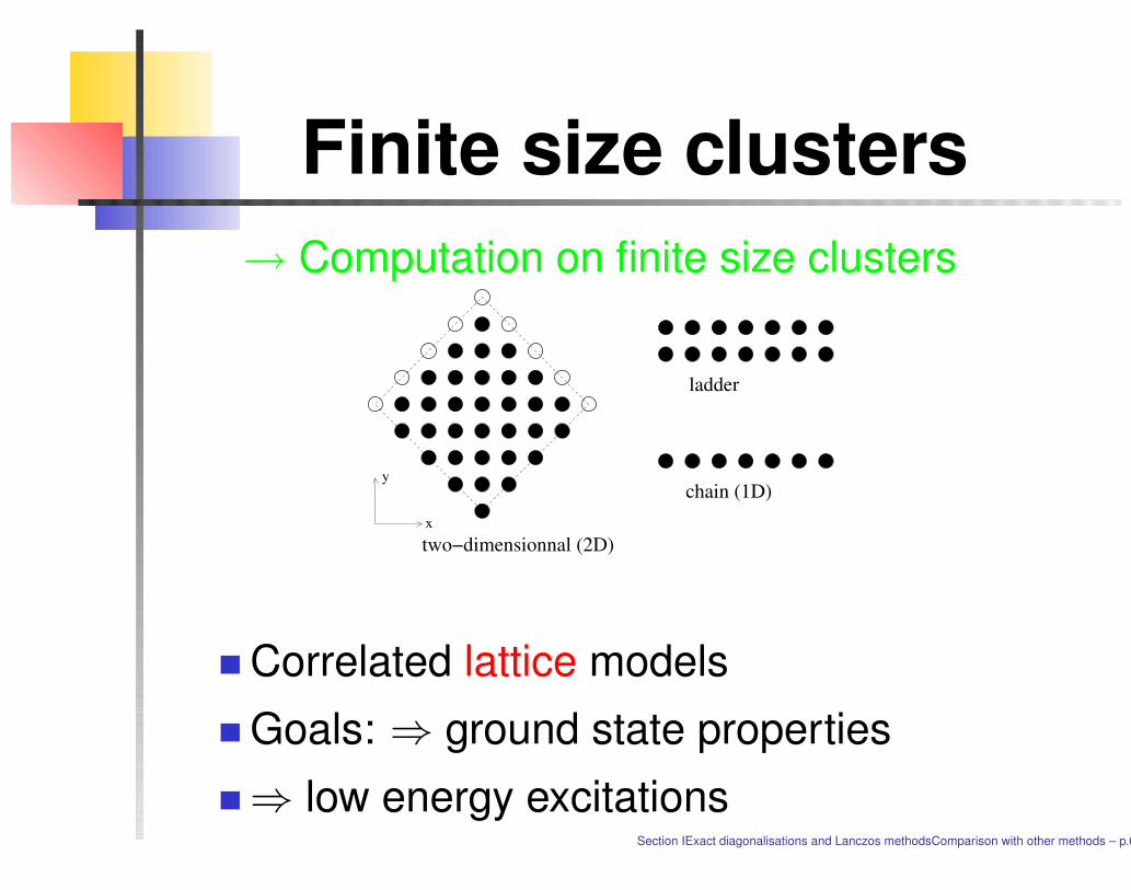
Finite size clusters→ Computation on finite size clusters

ladder

chain (1D)x

y

two−dimensionnal (2D)

Correlated lattice models

Goals: ⇒ ground state properties

⇒ low energy excitationsSection IExact diagonalisations and Lanczos methodsComparison with other methods – p.6

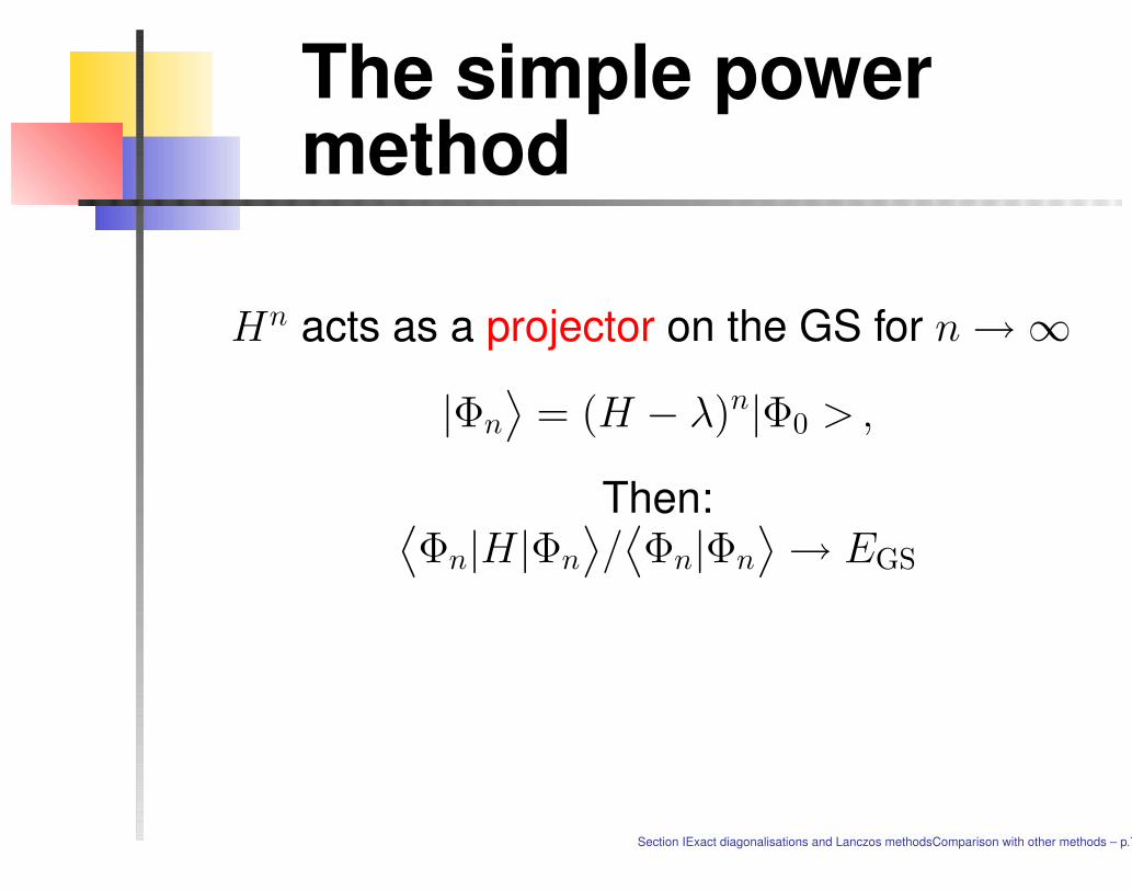
The simple powermethod

Hn acts as a projector on the GS for n → ∞

|Φn

⟩

= (H − λ)n|Φ0 > ,

Then:⟨

Φn|H|Φn

⟩

/⟨

Φn|Φn

⟩

→ EGS


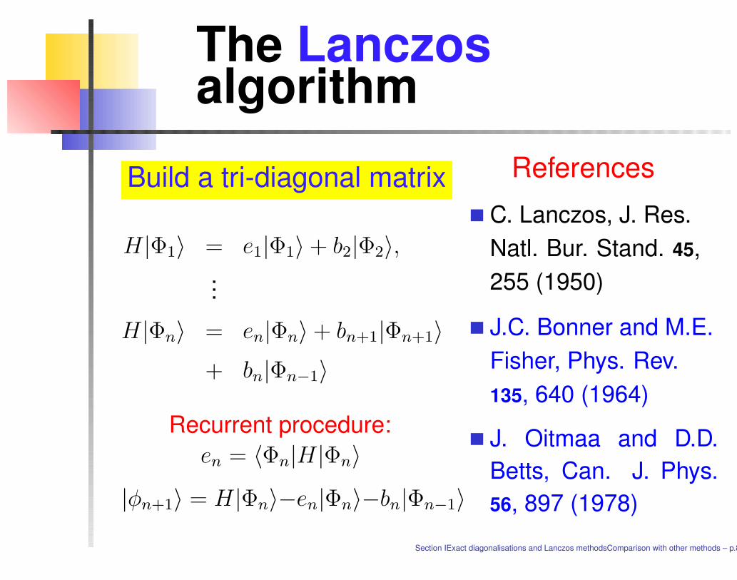
The Lanczosalgorithm

Build a tri-diagonal matrix

H|Φ1〉 = e1|Φ1〉 + b2|Φ2〉,...

H|Φn〉 = en|Φn〉 + bn+1|Φn+1〉

+ bn|Φn−1〉

Recurrent procedure:en = 〈Φn|H|Φn〉

|φn+1〉 = H|Φn〉−en|Φn〉−bn|Φn−1〉

References

C. Lanczos, J. Res.Natl. Bur. Stand. 45,255 (1950)

J.C. Bonner and M.E.Fisher, Phys. Rev.135, 640 (1964)

J. Oitmaa and D.D.Betts, Can. J. Phys.56, 897 (1978)


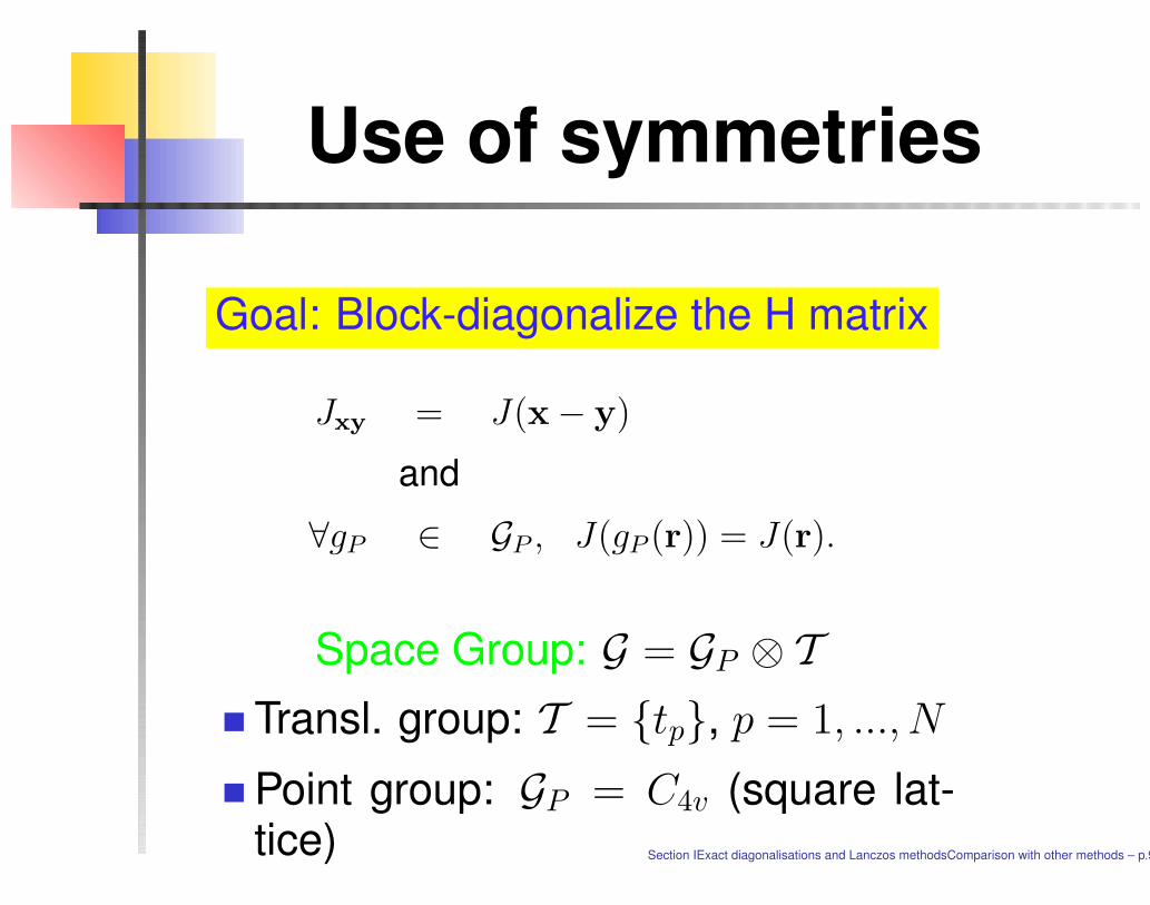
Use of symmetries

Goal: Block-diagonalize the H matrix

Jxy = J(x − y)

and

∀gP ∈ GP , J(gP (r)) = J(r).

Space Group: G = GP ⊗ T

Transl. group: T = {tp}, p = 1, ..., N

Point group: GP = C4v (square lat-tice) Section IExact diagonalisations and Lanczos methodsComparison with other methods – p.9

A simple example:the 2D t-J model

N=26 N=32

Nh /√

N ×√

N Hilbert space for SZ = Smin

ZSymmetry group Reduced HS

1 / 4 × 4 102 960 T16 6 435

1 /√

26 ×√

26 135 207 800 T26 5 200 300

1 /√

32 ×√

32 9 617 286 240 T32 ⊗ C4v 37 596 701∗

4 /√

26 ×√

26 10 546 208 400 T26 ⊗ C4 ⊗ I2 50 717 244


Use of "Blocktheorem"

K =∑

µ nµKµ ,

where Kµ reciprocal lattice vectorsKµ = 2π

N Tµ ∧ ez

GPK, little group of K (GP

K ⊂ GP ), containinggP such thatgP (K) = K .

The relevant subgroup of G:GK = GP

K ⊗ T .


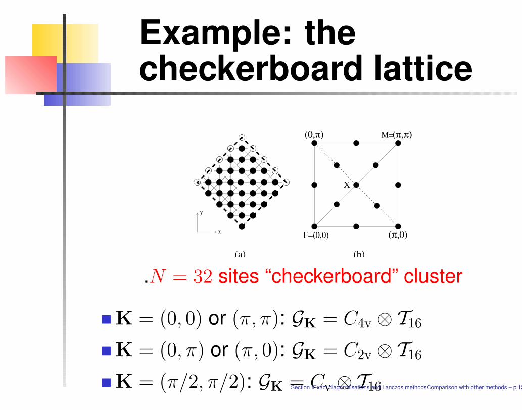
Example: thecheckerboard lattice

x

y

(a) (b)

Γ=(0,0)

(π,π)(0,π) M=

(π,0)

X

.N = 32 sites “checkerboard” cluster

K = (0, 0) or (π, π): GK = C4v ⊗ T16

K = (0, π) or (π, 0): GK = C2v ⊗ T16

K = (π/2, π/2): GK = Cv ⊗ T16Section IExact diagonalisations and Lanczos methodsComparison with other methods – p.12

Change boundaryconditions

- translation vectors of the formTµ = (0, ..., 0, Lµ, 0, ..., 0)

- flux Φ (in unit of the flux quantum) through onehole of d-dimensional torus→ twist in the boundary conditions alongdirection eµ:

txy c†x,scy,s → txy c†x,scy,s exp (2iπΦ

Lµ(x − y) · eµ)


Finite size scaling:Simple example: a one dimensionalsystem of correlated fermions


1D correlatedfermions: Hubbardchain

1D systems: spin and charge collective modeswith velocities uρ and uσ

Density of state: N(ω) ∼ |ω|α

α and Kρ non-universal exponents:α = 1

4(Kρ + 1Kρ

− 2)

Practical formula: πD = 2uρKρ

→ uρ and D obtained on finite systems:

"Drude weight": D = ∂2(E0/L)∂φ2 where φ = 2πΦ

L .

Velocity uρ: ∆E between k = 0 and k = 2π/Leigen-states Section IExact diagonalisations and Lanczos methodsComparison with other methods – p.15

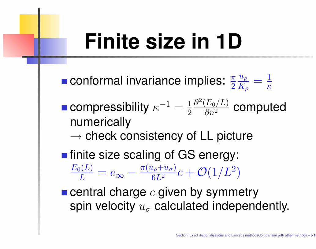
Finite size in 1D

conformal invariance implies: π2

uρ

Kρ= 1

κ

compressibility κ−1 = 12

∂2(E0/L)∂n2 computed

numerically→ check consistency of LL picture

finite size scaling of GS energy:E0(L)

L = e∞ − π(uρ+uσ)6L2 c + O(1/L2)

central charge c given by symmetryspin velocity uσ calculated independently.


Results &comparison with BA

Spinless fermion chain (t-V model) exactlysolvable by Bethe-Ansatz (n = 1/2)

Note: periodic boundary conditions used

0 0.002 0.004 0.006 0.008 1/L2

0.75

0.76

0.77

0.78

K

Kkkk

KDDD

0 0.5 1 1.5 2V

0.5

0.6

0.7

0.8

0.9

1

Krho

S. Capponi, Thèse 1999 (Toulouse)Section IExact diagonalisations and Lanczos methodsComparison with other methods – p.17

Partial summaryAdvantages

Non-perturbative method !!

Comparisons toexperiments:

Fits → microscopicparameters

Structure factors(ordering, etc...)

Thermodynamics

Spectroscopies(ARPES, INS, σ(ω),...)

Versatile method !Extensions to many

models - e.g. modelswith phonons

Limitations

Small clusters !!

Simple models(with few degreeof freedom/ / site)


A little practice:How to implement the Lanczos methodon a computer ?


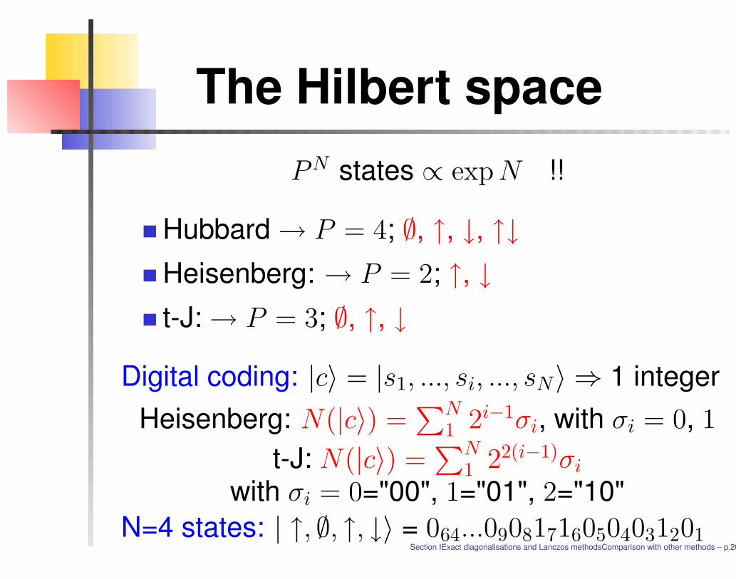
The Hilbert spacePN states ∝ exp N !!

Hubbard → P = 4; ∅, ↑, ↓, ↑↓

Heisenberg: → P = 2; ↑, ↓

t-J: → P = 3; ∅, ↑, ↓

Digital coding: |c〉 = |s1, ..., si, ..., sN〉 ⇒ 1 integerHeisenberg: N(|c〉) =

∑N1 2i−1σi, with σi = 0, 1

t-J: N(|c〉) =∑N

1 22(i−1)σi

with σi = 0="00", 1="01", 2="10"N=4 states: | ↑, ∅, ↑, ↓〉 = 064...090817160504031201


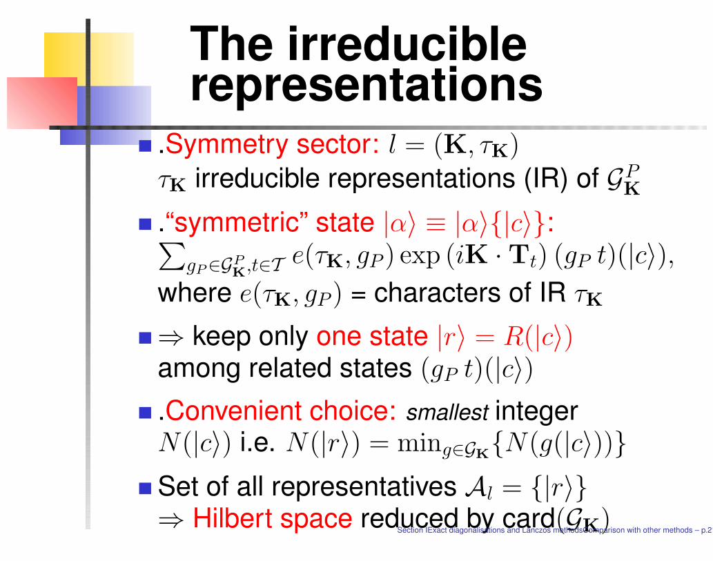
The irreduciblerepresentations

.Symmetry sector: l = (K, τK)

τK irreducible representations (IR) of GPK

.“symmetric” state |α〉 ≡ |α〉{|c〉}:∑

gP∈GPK

,t∈T e(τK, gP ) exp (iK · Tt) (gP t)(|c〉),

where e(τK, gP ) = characters of IR τK

⇒ keep only one state |r〉 = R(|c〉)among related states (gP t)(|c〉)

.Convenient choice: smallest integerN(|c〉) i.e. N(|r〉) = ming∈GK

{N(g(|c〉))}

Set of all representatives Al = {|r〉}⇒ Hilbert space reduced by card(GK)


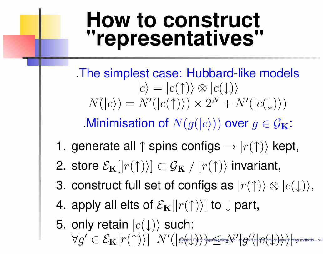
How to construct"representatives"

.The simplest case: Hubbard-like models|c〉 = |c(↑)〉 ⊗ |c(↓)〉

N(|c〉) = N ′(|c(↑)〉) × 2N + N ′(|c(↓)〉)

.Minimisation of N(g(|c〉)) over g ∈ GK:

1. generate all ↑ spins configs → |r(↑)〉 kept,

2. store EK[|r(↑)〉] ⊂ GK / |r(↑)〉 invariant,

3. construct full set of configs as |r(↑)〉 ⊗ |c(↓)〉,

4. apply all elts of EK[|r(↑)〉] to ↓ part,

5. only retain |c(↓)〉 such:∀g′ ∈ EK[r(↑)〉] N ′(|c(↓)〉) ≤ N ′[g′(|c(↓)〉)] .Section IExact diagonalisations and Lanczos methodsComparison with other methods – p.22

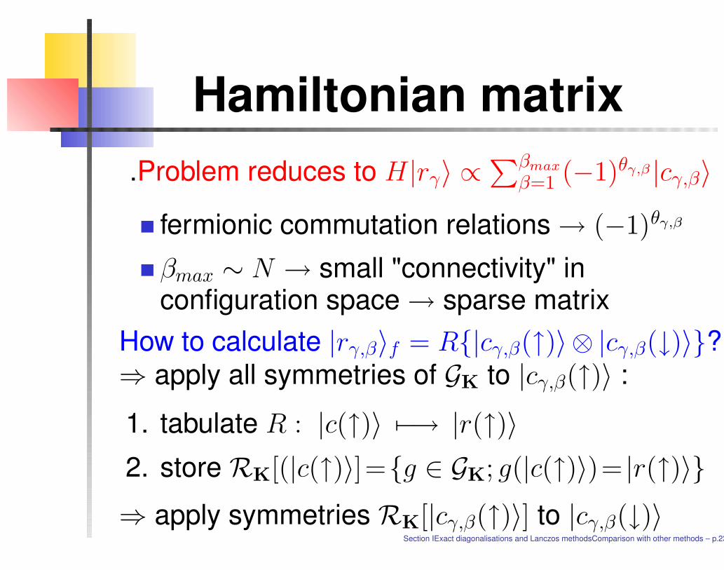
Hamiltonian matrix.Problem reduces to H|rγ〉 ∝

∑βmax

β=1 (−1)θγ,β |cγ,β〉

fermionic commutation relations → (−1)θγ,β

βmax ∼ N → small "connectivity" inconfiguration space → sparse matrix

How to calculate |rγ,β〉f = R{|cγ,β(↑)〉 ⊗ |cγ,β(↓)〉}?⇒ apply all symmetries of GK to |cγ,β(↑)〉 :

1. tabulate R : |c(↑)〉 7−→ |r(↑)〉

2. store RK[(|c(↑)〉]={g ∈ GK; g(|c(↑)〉)= |r(↑)〉}

⇒ apply symmetries RK[|cγ,β(↑)〉] to |cγ,β(↓)〉Section IExact diagonalisations and Lanczos methodsComparison with other methods – p.23

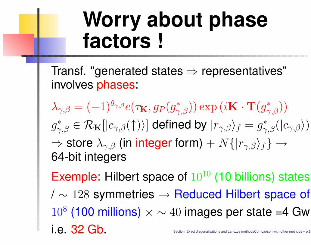
Worry about phasefactors !

Transf. "generated states ⇒ representatives"involves phases:

λγ,β = (−1)θγ,βe(τK, gP (g∗γ,β)) exp (iK · T(g∗γ,β))

g∗γ,β ∈ RK[|cγ,β(↑)〉] defined by |rγ,β〉f = g∗γ,β(|cγ,β〉)

⇒ store λγ,β (in integer form) + N{|rγ,β〉f} →64-bit integers

Exemple: Hilbert space of 1010 (10 billions) states/ ∼ 128 symmetries → Reduced Hilbert space of108 (100 millions) × ∼ 40 images per state =4 Gwi.e. 32 Gb. Section IExact diagonalisations and Lanczos methodsComparison with other methods – p.24

The link with experiments:

Dynamical correlations calculated

with Lanczos


Computing DynamicsCorrelations - Outline

1. The continued-fraction method

2. Experimentally accessible fluctua-tions

3. The convergence of the method


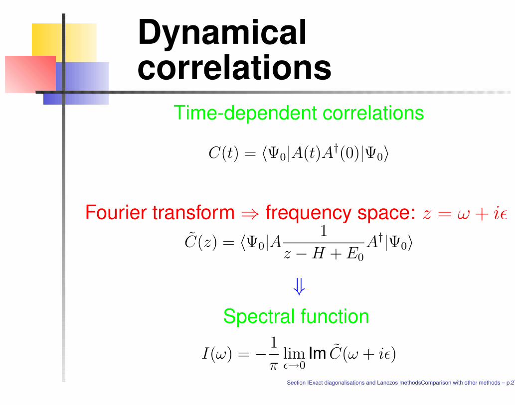
Dynamicalcorrelations

Time-dependent correlations

C(t) = 〈Ψ0|A(t)A†(0)|Ψ0〉

Fourier transform ⇒ frequency space: z = ω + iε

C(z) = 〈Ψ0|A1

z − H + E0

A†|Ψ0〉

⇓

Spectral function

I(ω) = −1

πlimε→0

Im C(ω + iε)


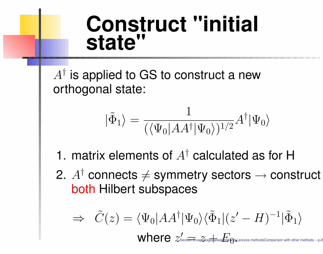
Construct "initialstate"

A† is applied to GS to construct a neworthogonal state:

|Φ1〉 =1

(〈Ψ0|AA†|Ψ0〉)1/2A†|Ψ0〉

1. matrix elements of A† calculated as for H

2. A† connects 6= symmetry sectors → constructboth Hilbert subspaces

⇒ C(z) = 〈Ψ0|AA†|Ψ0〉〈Φ1|(z′ − H)−1|Φ1〉

where z′ = z + E0.Section IExact diagonalisations and Lanczos methodsComparison with other methods – p.28

second Lanczositerative procedure

Starting with |Φ1〉 as an initial state:

z′ − H =

z′ − e1 −b2 . . . 0

−b2. . . . . . ...

... . . . . . . −bM

0 . . . −bM z′ − eM

(1)

→ matrix expressed in the new basis {|Φn〉} withnew choice |Φ1〉 = |Φ1〉.


Recurrence relationsStraightforwardly:

C(z) = 〈Ψ0|AA†|Ψ0〉D2

D1,

where Dn is defined as Dn = det ∆n

∆n is the (M − n + 1) × (M − n + 1) matrix:

∆n =

z′ − en −bn+1 . . . 0

−bn+1. . . . . . ...

... . . . . . . −bM

0 . . . −bM z′ − eM

(2)


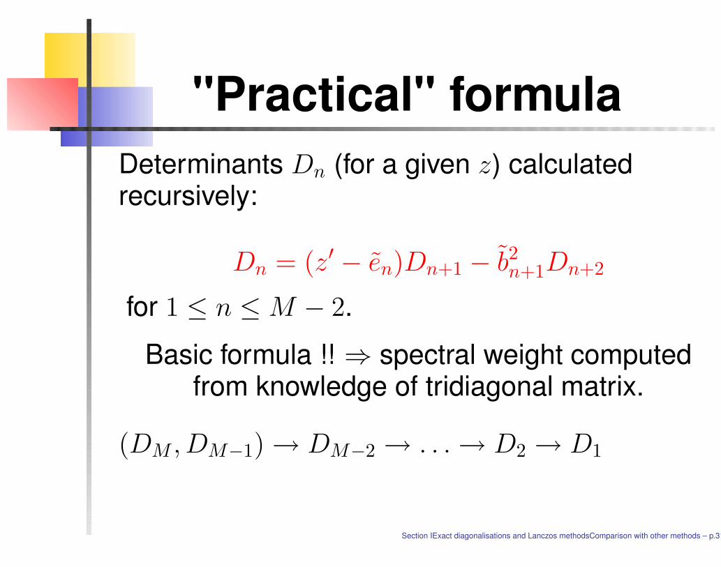
"Practical" formulaDeterminants Dn (for a given z) calculatedrecursively:

Dn = (z′ − en)Dn+1 − b2n+1Dn+2

for 1 ≤ n ≤ M − 2.

Basic formula !! ⇒ spectral weight computedfrom knowledge of tridiagonal matrix.

(DM , DM−1) → DM−2 → . . . → D2 → D1


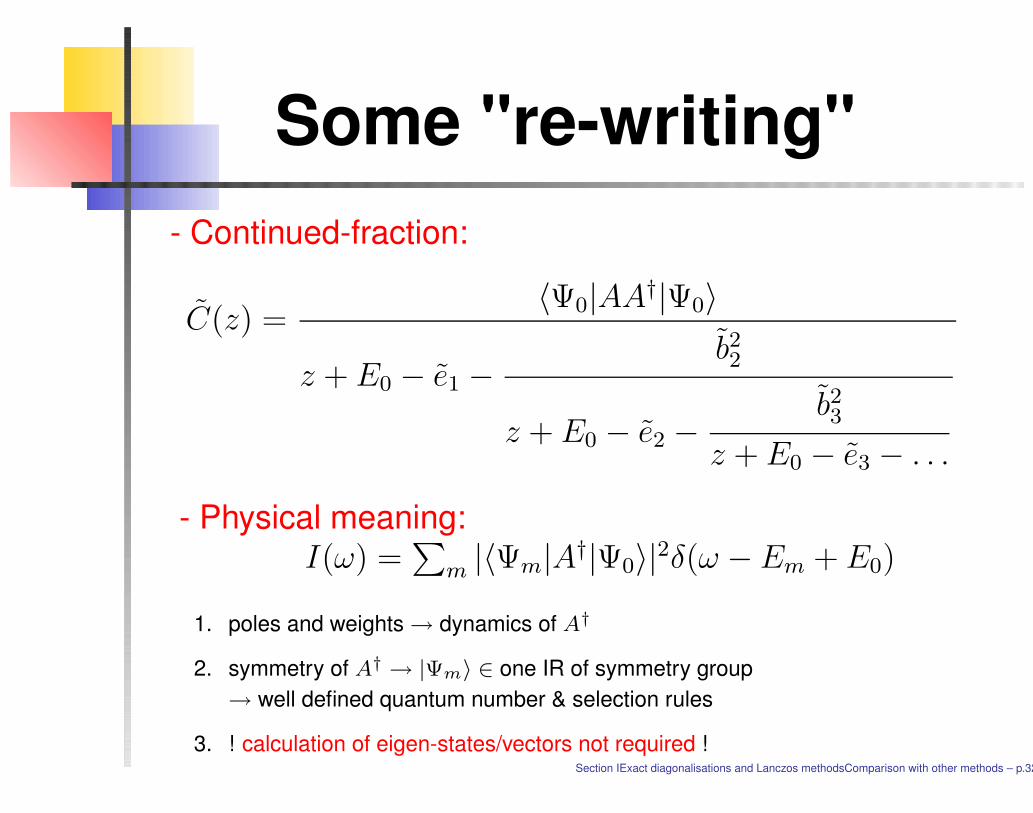
Some "re-writing"- Continued-fraction:

C(z) =〈Ψ0|AA†|Ψ0〉

z + E0 − e1 −b22

z + E0 − e2 −b23

z + E0 − e3 − . . .

- Physical meaning:I(ω) =

∑

m |〈Ψm|A†|Ψ0〉|

2δ(ω − Em + E0)

1. poles and weights → dynamics of A†

2. symmetry of A† → |Ψm〉 ∈ one IR of symmetry group→ well defined quantum number & selection rules

3. ! calculation of eigen-states/vectors not required !Section IExact diagonalisations and Lanczos methodsComparison with other methods – p.32

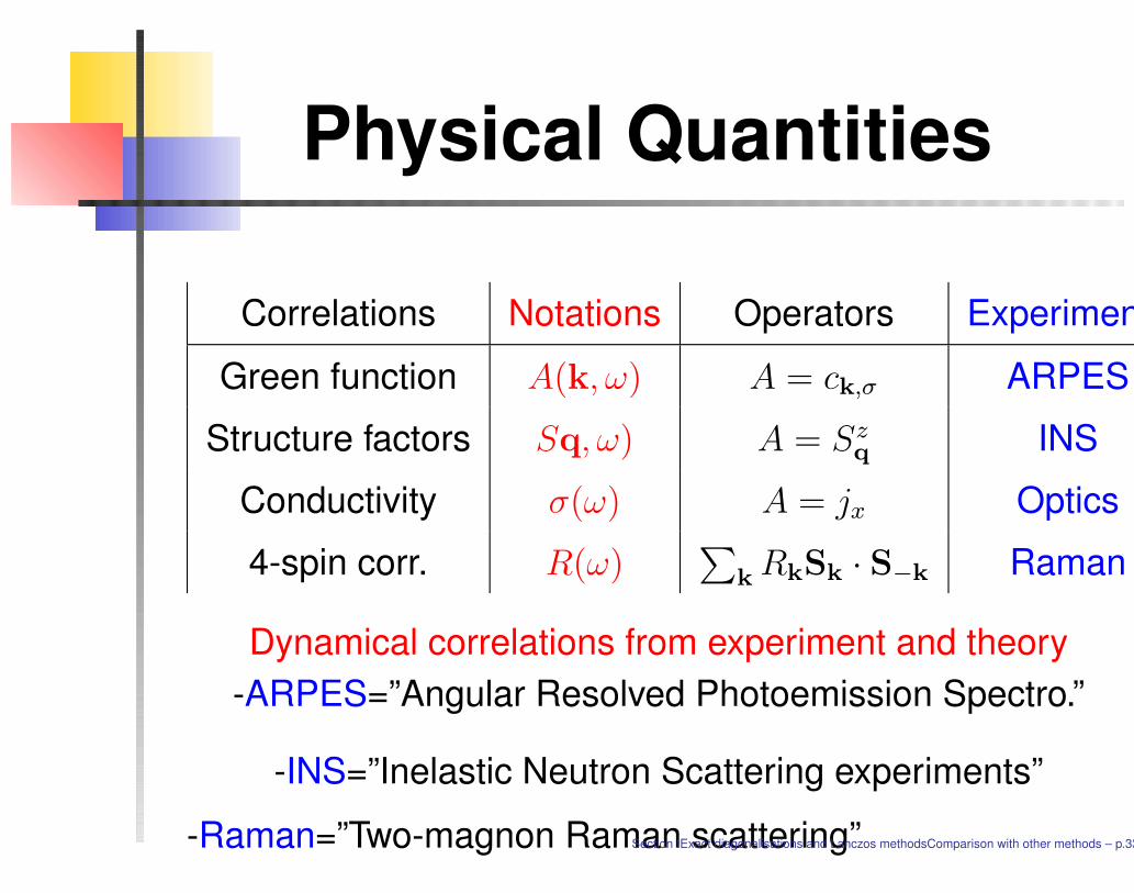
Physical Quantities

Correlations Notations Operators Experiments

Green function A(k, ω) A = ck,σ ARPES

Structure factors Sq, ω) A = Szq INS

Conductivity σ(ω) A = jx Optics

4-spin corr. R(ω)∑

k RkSk · S−k Raman

Dynamical correlations from experiment and theory-ARPES=”Angular Resolved Photoemission Spectro.”

-INS=”Inelastic Neutron Scattering experiments”

-Raman=”Two-magnon Raman scattering”Section IExact diagonalisations and Lanczos methodsComparison with other methods – p.33

Problems ofconvergence ?

A priori, should worry about:

1. role of M , the # of Lanczos iterations ?

2. role of the imaginary part ε in z = ω + iε ?

3. role of system size ?

In fact, numerically EXACT results for a given sys-tem size


Convergence withsize

Ex.: single hole in a 2D antiferromagnet Localdensity of state: N(ω) =

∑

k A(k, ω)

D.P. et al., PRB (1993)

|Ψ0

⟩

= Heisenberg GSA = ciσ: hole creationUse of 2D "tilted" clus-ters: N = n2 + m2

T1 = (n, m)T2 = (−m, n)|T1| = |T2| &T1 · T2 = 0


Other numerical methods:

CORE method – Density Matrix

Renormalisation Group (DMRG) –

Quantum Monte Carlo (QMC)Comparison with Lanczos


COntractorREnormalisation

CORE method (Auerbach et al., Capponi et al.)

1. “Macrosites” (= rungs, plaquettes, etc...) → < de-grees of freedom

2. construct effective H with longer-range & m-body in-teractions


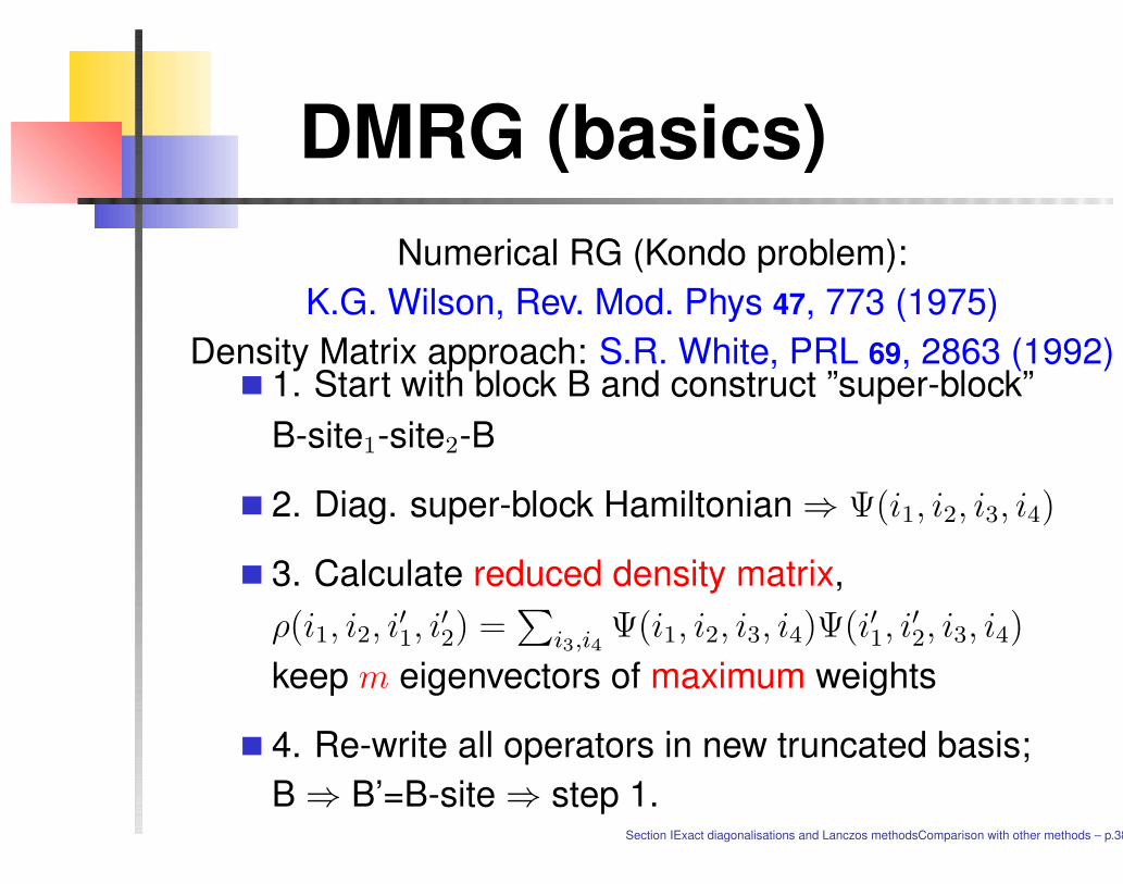
DMRG (basics)Numerical RG (Kondo problem):

K.G. Wilson, Rev. Mod. Phys 47, 773 (1975)Density Matrix approach: S.R. White, PRL 69, 2863 (1992)

1. Start with block B and construct ”super-block”B-site1-site2-B

2. Diag. super-block Hamiltonian ⇒ Ψ(i1, i2, i3, i4)

3. Calculate reduced density matrix,ρ(i1, i2, i

′1, i

′2) =

∑

i3,i4Ψ(i1, i2, i3, i4)Ψ(i′1, i

′2, i3, i4)

keep m eigenvectors of maximum weights

4. Re-write all operators in new truncated basis;B ⇒ B’=B-site ⇒ step 1.


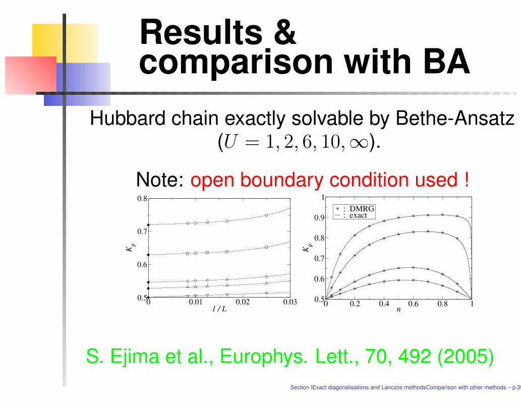
Results &comparison with BA

Hubbard chain exactly solvable by Bethe-Ansatz(U = 1, 2, 6, 10,∞).

Note: open boundary condition used !

0 0.01 0.02 0.031 / L

0.5

0.6

0.7

0.8

Kρ

0 0.2 0.4 0.6 0.8 1n

0.5

0.6

0.7

0.8

0.9

1

Kρ

: DMRG: exact

S. Ejima et al., Europhys. Lett., 70, 492 (2005)Section IExact diagonalisations and Lanczos methodsComparison with other methods – p.39

Quantum MonteCarlo methods(basics)

1. Metropolis algorithm

2. World-line algorithms

3. Continuous-time & SSE

4. Determinantal MC (fermions)


Monte Carlo method"Non-local updates for QMC simulations",M. Troyer et al., p.156 in "The Monte Carlo

Method in the Physical Sciences", AIP Conf.Proc., Vol. 690 (2003)

- Monte Carlo: iterative stochastic procedure inconfiguration space

- Metropolis algorithm to sample probabilitydistrib. p(i):

P (i → j) = min[1, p(j)p(i) ]

Metropolis, Rosenbluth, Rosenbluth, Teller & Teller (1953)


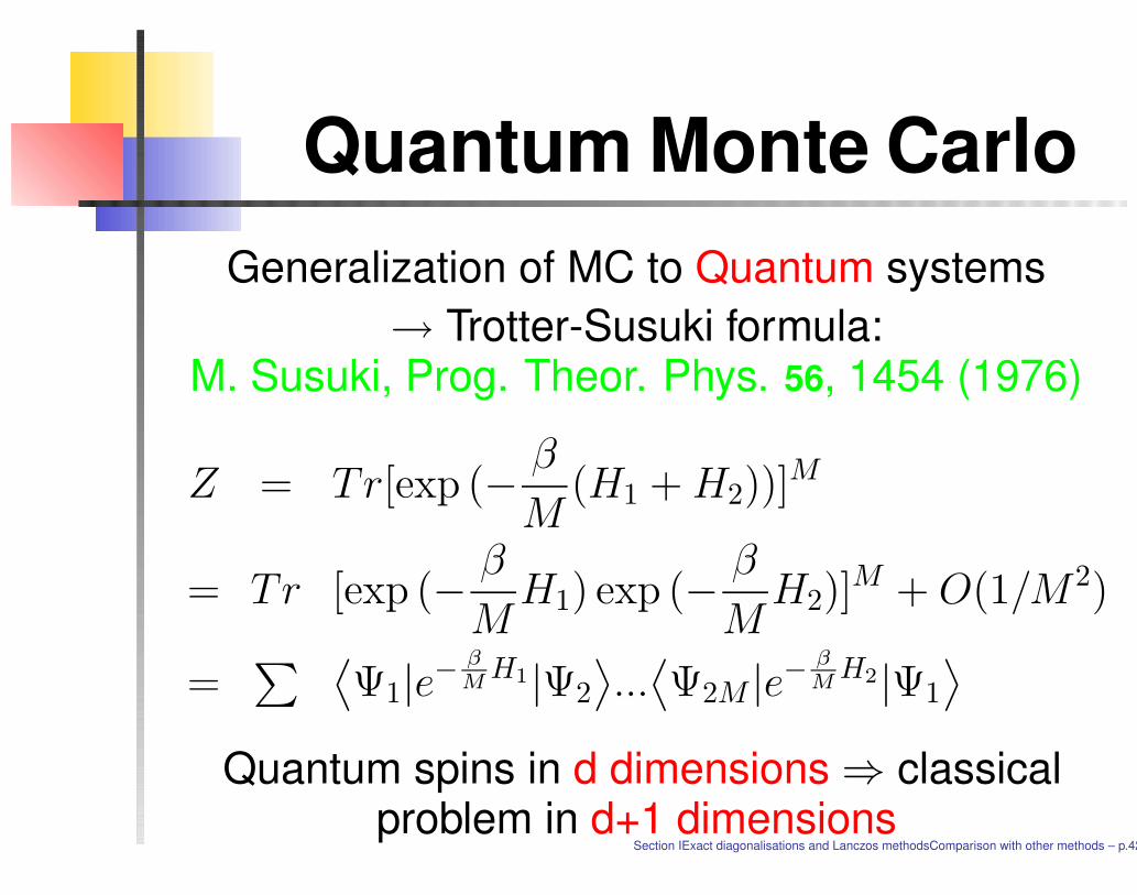
Quantum Monte CarloGeneralization of MC to Quantum systems

→ Trotter-Susuki formula:M. Susuki, Prog. Theor. Phys. 56, 1454 (1976)

Z = Tr[exp (−β

M(H1 + H2))]

M

= Tr [exp (−β

MH1) exp (−

β

MH2)]

M + O(1/M 2)

=∑

⟨

Ψ1|e− β

MH1|Ψ2

⟩

...⟨

Ψ2M |e−βM

H2|Ψ1

⟩

Quantum spins in d dimensions ⇒ classicalproblem in d+1 dimensions


World-linerepresentations

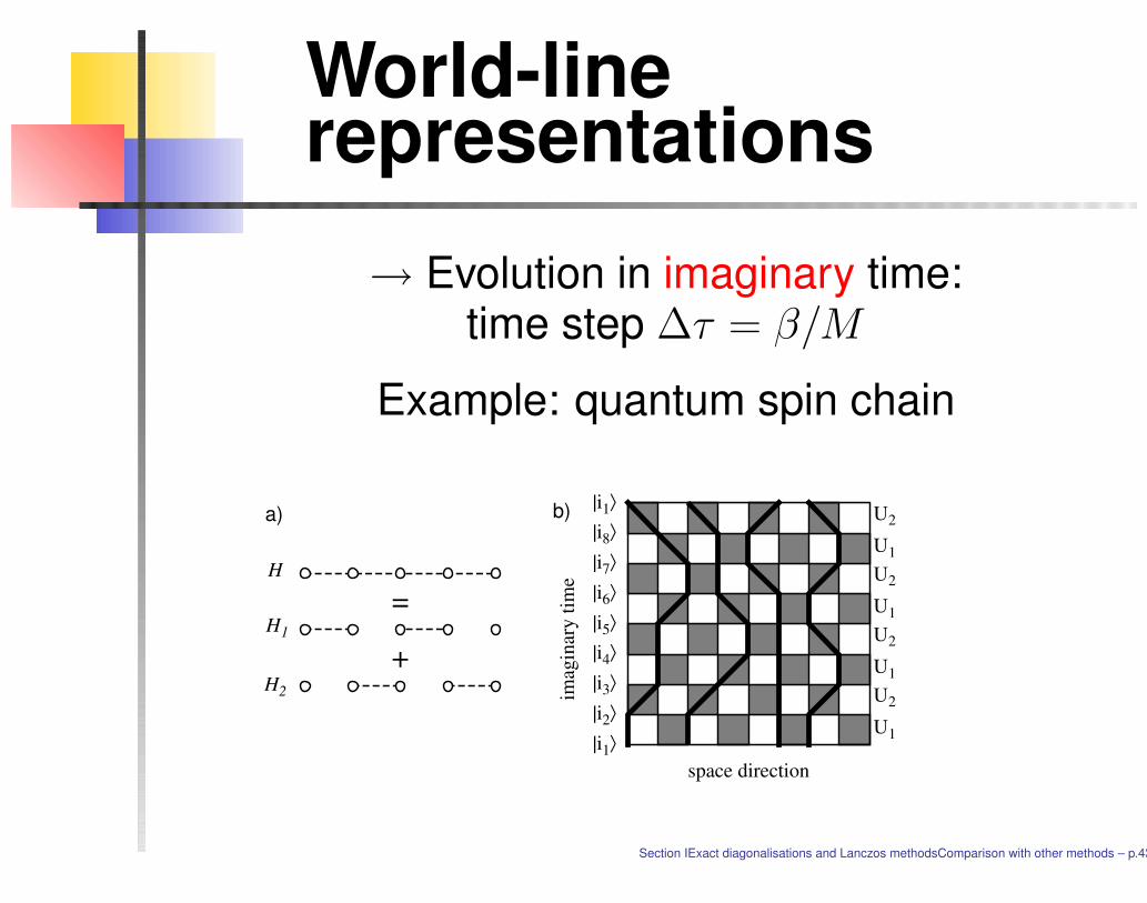
→ Evolution in imaginary time:time step ∆τ = β/M

Example: quantum spin chain

=

+

H

H1

H2

a)

space direction

imag

inar

y tim

e

U2

U1

U2

U1

U2

U1

U2

U1

|i1⟩|i2⟩|i3⟩|i4⟩|i5⟩|i6⟩|i7⟩|i8⟩|i1⟩b)


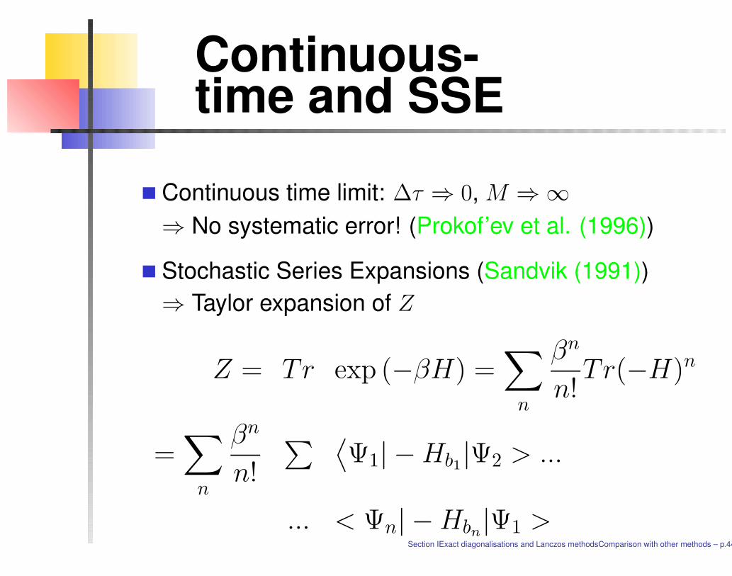
Continuous-time and SSE

Continuous time limit: ∆τ ⇒ 0, M ⇒ ∞

⇒ No systematic error! (Prokof’ev et al. (1996))

Stochastic Series Expansions (Sandvik (1991))⇒ Taylor expansion of Z

Z = Tr exp (−βH) =∑

n

βn

n!Tr(−H)n

=∑

n

βn

n!

∑⟨

Ψ1| − Hb1|Ψ2 > ...

... < Ψn| − Hbn|Ψ1 >


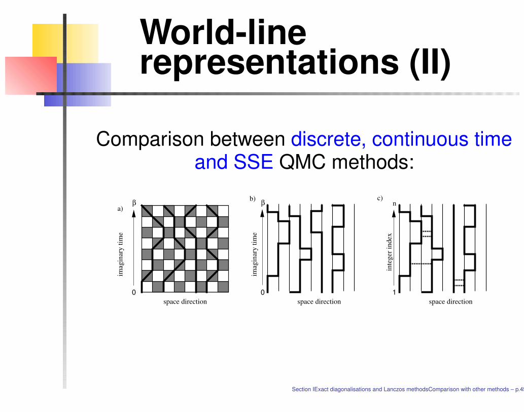
World-linerepresentations (II)

Comparison between discrete, continuous timeand SSE QMC methods:

space direction

imag

inar

y tim

e

a)

space direction

inte

ger i

ndex

c)

0

β

1

n

space direction

imag

inar

y tim

e

b)

0

β


How to simulatefermions ?

Fermionic case - J.H. Hirsch, 1985Hubbard-Stratonovich transformation

Idea: (i) use Trotter formula for"decoupling" K (kin.) & V (int.)(ii) decouple interaction term

(iii) integrate out fermionic variables

e−∆τUni,↑ni,↓ ∝∑

s=±1 e−∆τsi,lλ(ni,↑−ni,↓)

Z =∑

s=±1 detM+(s)detM−(s)


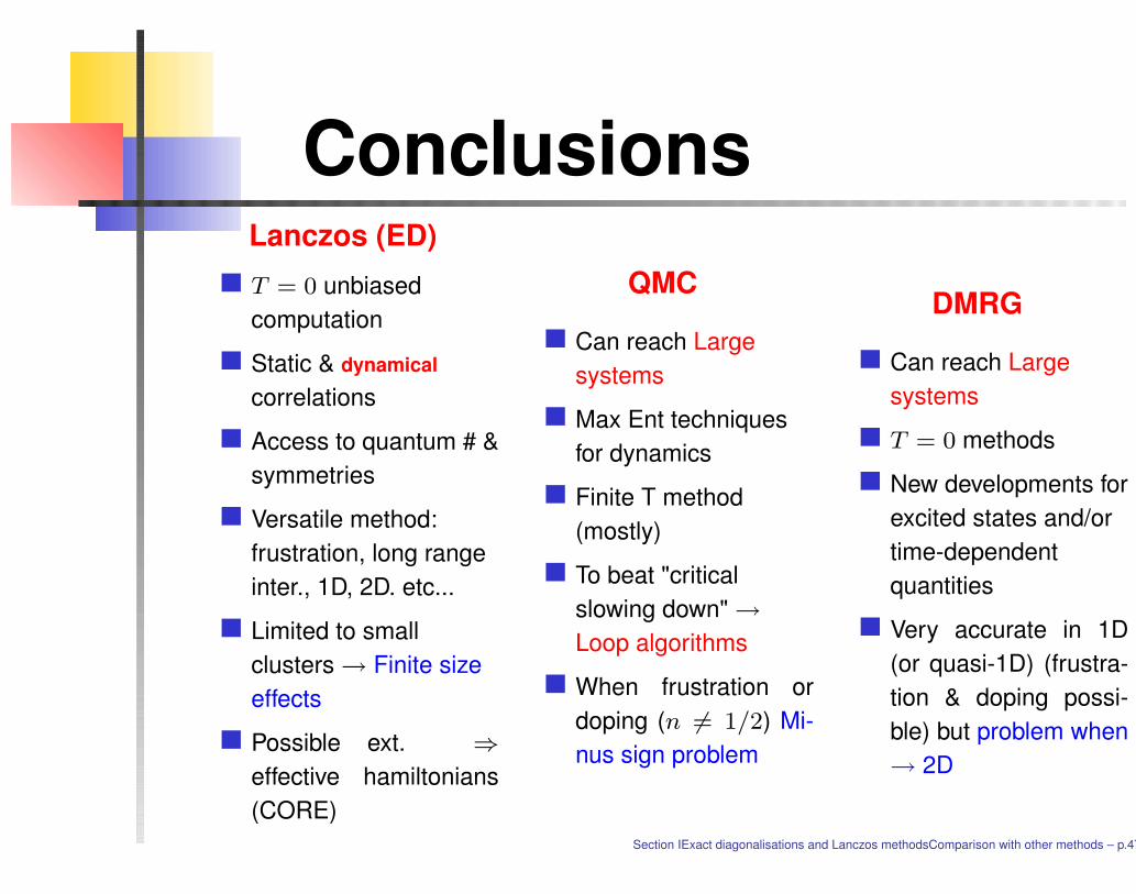
ConclusionsLanczos (ED)

T = 0 unbiasedcomputation

Static & dynamical

correlations

Access to quantum # &symmetries

Versatile method:frustration, long rangeinter., 1D, 2D. etc...

Limited to smallclusters → Finite sizeeffects

Possible ext. ⇒effective hamiltonians(CORE)

QMC

Can reach Largesystems

Max Ent techniquesfor dynamics

Finite T method(mostly)

To beat "criticalslowing down" →Loop algorithms

When frustration ordoping (n 6= 1/2) Mi-nus sign problem

DMRG

Can reach Largesystems

T = 0 methods

New developments forexcited states and/ortime-dependentquantities

Very accurate in 1D(or quasi-1D) (frustra-tion & doping possi-ble) but problem when→ 2D


Date post:	17-Jul-2018
Category:	Documents
Upload:	phamhanh
View:	220 times
Download:	0 times

Section I Exact diagonalisations and Lanczos methods...

Documents