Segmenting Point Sets

Ichitaro Yamazaki∗

yamazaki@cs.ucdavis.eduVijay Natarajan†

vijayn@ucdavis.eduZhaojun Bai∗

bai@cs.ucdavis.eduBernd Hamann†,∗

hamann@cs.ucdavis.edu

Institute for Data Analysis and Visualization (IDAV)†

and Department of Computer Science∗

University of California, Davis, California 95616

Abstract

Extracting features from point sets is becoming in-creasingly important for purposes like model classifica-tion, matching, and exploration. We introduce a tech-nique for segmenting a point-sampled surface into dis-tinct features without explicit construction of a meshor other surface representation. Our approach achievescomputational efficiency through a three-phase segmen-tation process. The first phase of the process uses a topo-logical approach to define features and coarsens the input,resulting in a set of supernodes, each one represent-ing a collection of input points. A graph cut is employedin the second phase to bisect the set of supernodes. Sim-ilarity between supernodes is computed as a weightedcombination of geodesic distances and connectivity. Re-peated application of the graph cut results in a hier-archical segmentation of the point input. In the lastphase, a segmentation of the original point set is con-structed by refining the segmentation of the supernodesbased on their associated feature sizes. We apply our seg-mentation algorithm on laser-scanned models to eval-uate its ability to capture geometric features in com-plex data sets.

Keywords: point sets, sampling, features, geodesic dis-tance, normalized cut, spectral analysis, hierarchical seg-mentation.

1. Introduction

Recent developments in scanning technologies haveled to a substantial increase in the number of avail-able surface models. Features in a surface model areits distinct parts that characterize the surface model.Examples of features are legs of a horse or fingers in ahand. We propose a new definition of features and de-scribe an efficient three-phase segmentation process for

partitioning a given point-sampled surface into distinctparts without explicit construction of a triangle mesh.In the first phase, we use the intrinsic dimension of thepoint sample, which is typically lower than the dimen-sion of the embedding space, to identify sets of pointsthat constitute distinct features. We adopt a topologi-cal approach to define features: a discrete function andits associated gradient flow field are constructed for theinput point set. The discrete function measures the cen-trality of each point within the surface. A collection ofpoints that flow into a common sink of this flow fieldconstitute a feature. Each sink represents a feature andis called a supernode. In the second phase, we use spec-tral analysis to bisect a graph constructed over the su-pernodes. Repeated application of this bisection resultsin a hierarchical segmentation of the surface point set.This segmentation is refined in the third phase, wheresegments with insignificantly small features are mergedinto a neighboring segment with a larger feature. Ourapproach has the following advantages:

• Efficiency. Point primitives support simple andflexible modeling of complex shapes and are there-fore increasingly being used to represent surfaces[25, 34]. We work directly with the point primi-tives used to represent the surface without explicitconstruction of a mesh. This approach leads to ef-ficient usage of storage and computing resourcesto segment a point set.

• Simple implementation. Our program modules forall three phases of segmentation consist of a totalof around 350 lines of code.

• Hierarchy. A hierarchical segmentation supportsmultiple views of the partition based on a desiredlevel of detail.

• Extension to higher dimensions and non-Euclideanspaces. Since we operate only on point primitives,all three phases of the segmentation can be ap-plied to higher-dimensional data. Also, the embed-

ding space is not restricted to be Euclidean. Wemerely require the points to be embedded in a met-ric space. Our method can potentially be used tosegment point sets lying on a sub-manifold withina high-dimensional space [31].

2. Related Work

Current approaches to feature-based segmentationtypically require that a surface model is provided ex-plicitly via a triangle mesh [14, 18, 24, 32] or that amesh is procedurally constructed [4].

Segmenting a model into its distinct parts and ex-tracting its features are crucial for several applicationslike shape recognition, classification, matching, sim-plification, analysis, morphing, retrieval, and surfacereconstruction [7, 9, 12, 16, 19, 28]. Numerous sur-face segmentation methods have been developed basedon techniques from computer vision, load partitioningin finite element methods (FEM), point set cluster-ing in statistics, and machine learning. These methodscan be broadly classified into two categories based ontheir objective, namely patch-type segmentation andpart-type segmentation [29]. Patch-type methods ob-tain segments that are topological disks whereas part-type methods partition a surface into segments thatcorrespond to features.

Existing surface segmentation methods typically as-sume a surface to be represented by mesh. Various ap-proaches have been used successfully for mesh segmen-tation: watershed segmentation simulates the accumu-lation of water into basins [19, 24]; spectral clusteringmethods analyze an affinity matrix that stores mea-sures of similarity between all pairs of mesh faces inorder to partition the mesh [10, 18]; mesh partitioningmethods are a crucial ingredient in various load balanc-ing algorithms, where the goal is to partition the inputinto independent sets that can be processed in paral-lel [27]; and point clustering methods are used for ef-ficient organization of data with applications in infor-mation retrieval [15].

The method described by Dey et. al. [4] and the firstphase of our method both initially identify local max-ima of a discrete function. Though these local maximaconstitute distinct features, they are computed differ-ently. Dey et al. describe the discrete function on an ex-plicitly computed three-dimensional mesh. We, on theother hand, define a discrete function over the pointsample. Points are assigned to a feature by Dey et al.based on the flows induced within the mesh whereaswe determine features based on gradient flow of thediscrete function. Since we work in a lower dimension,namely on the surface, our approach computes a seg-

mentation 5-7 times faster than their approach. Zhanget al. [33] propose a method to identify segments corre-sponding to local maxima of the average geodesic dis-tance function, which is similar to our method. Theyare, however, interested in obtaining a patch-type seg-mentation for surface parameterization. A features isidentified by growing a region based on the geodesicdistance from a local maximum and searching for a fea-ture boundary, which results in an abrupt increase inthe surrounded region. The approach of Katz and Tal[16] also decomposes a mesh using representative facesfor distinct features. These representative faces are cho-sen iteratively using a k-means algorithm. Faces are as-signed to a feature based on the geodesic distance be-tween the face and representative.

3. Three-phase Segmentation

Given a point-sampled surface as input, we want topartition the surface into distinct parts by associatingeach point with the feature that it belongs to. We pro-pose a three-phase process to perform this segmenta-tion:

1. Feature identification. In the first phase, we definefeatures using a topological approach. This phasesets the stage for performing hierarchical segmen-tation in an efficient manner by coarsening the in-put into supernodes. Each supernode representsa collection of input points that constitute a fea-ture.

2. Hierarchical segmentation. In the second phase, webisect the set of supernodes while ensuring thatsimilar supernodes remain together. Repeated ap-plication of this bisection step results in a hierar-chical segmentation of the input point set. A near-optimal bisection is computed by using spectralanalysis of a graph whose edge weights correspondto the similarity between the end point supern-odes. The second phase of segmentation processcan be applied directly to the input point set. How-ever, computing a near-optimal bisection is signif-icantly faster when applied on smaller sets of su-pernodes. Moreover, the first phase ensures that afeature lies within a single segment.

3. Refinement. In the third phase, we post-processthe segmentation to ensure that all segments con-tain at least one significant feature. Small-scalefeatures, that are present as individual segments,are merged with a neighboring segment.

In the following sections, we discuss these three phasesin detail and provide results of our experiments for var-ious laser scanned models.

4. Feature Identification

We use ideas from Morse theory to define featuresin the input. Morse theory was originally developed tostudy the relationship between the shape of a space andthe critical points of smooth functions defined on thespace [20, 21]. Recently, it has been successfully used toconstruct multi-resolution structures for the visualiza-tion of scalar field data [2, 11, 23]. Dey et al. adaptedideas from Morse theory for smooth functions to a dis-crete domain to segment 3D models [4]. The above ap-plications of Morse theory require an explicit represen-tation of the domain space, i.e., a triangle or tetrahe-dral mesh. We, on the other hand, work directly withpoint sets. We construct a discrete function f that mea-sures the centrality of a point within the surface. Thenotion of centrality has been studied in the context ofsocial networks [6] and more recently in the context ofshape matching [13]. In our segmentation process, cen-trality of a point p is defined as the average geodesicdistance from p to other points on the surface, and itmeasures the importance of the point to capture a fea-ture in the surface. A shortest path in a graph G thatconnects every point to its k-nearest neighbors approx-imates the geodesic distance between two points on thesurface when a sufficiently dense point-sampled surfaceis provided [31].

6

8

7

5

9

6

9a

b

Figure 1. Geodesic distance computation. Distance

between two points is given by the Euclidean metric in

the embedded space (left). A graph connecting every

point to its k-nearest neighbors for k = 3 (middle).

Shortest path between two points a and b approximat-

ing the geodesic distance (right).

A discrete gradient of f at an input point p is de-fined as

max|f(p) − f(q)|‖p − q‖2

among k-nearest neighbors q of p where ‖‖2 denotesthe Euclidean distance between p and q. Thus, discretegradient for an input point is defined by the edge inG that corresponds to the steepest ascent of functionf . In our segmentation process, sinks of this discrete

gradient flow field define distinct features, and they arecalled supernodes.

Figure 2. Features and their constituent points.

Left: two local maxima of the discrete function; mid-

dle: edges with steepest gradient are followed from

each point toward a local maximum; right: all points

grouped into two sets based on their associated lo-

cal maxima.

Given a point set P , the first phase of the segmen-tation approach proceeds as follows:

1. Store P in a kd-tree.

2. For each point p ∈ P , compute the k-nearestneighbors using a kd-tree [22].

3. Construct a weighted graph G over P whose edgesare given by the k-nearest neighbors resulting fromstep 2. Set the weight of an edge to the Euclideandistance between its end points.

4. Compute a discrete function f at each point p asthe average shortest distance from p to all pointsin G. Use Dijkstra’s shortest path algorithm [3] tocompute the distance between two points in G.

5. For each point p ∈ P , compute a discrete gradientflow by considering the edge incident on P alongwhich f increases maximally. Declare p a sink ifnone of its neighbors has a higher function value.

6. Follow the gradient flow field from each point p to-ward a sink, and include p into the feature identi-fied by its associated sink.

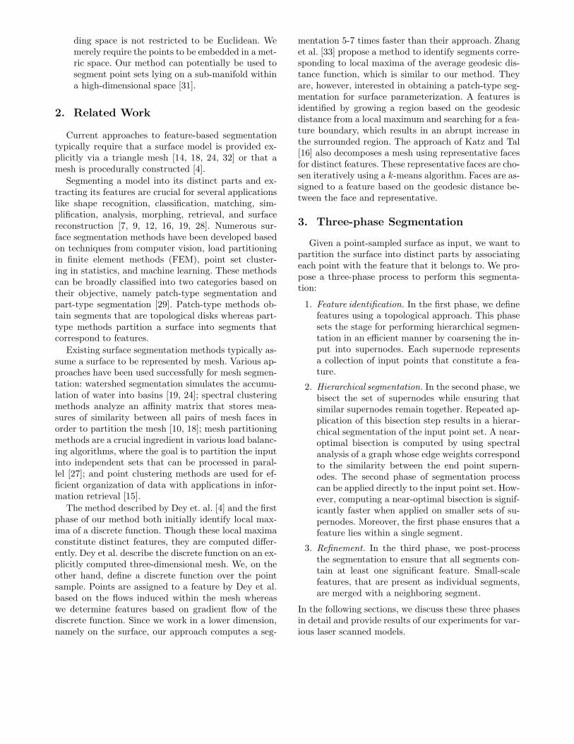
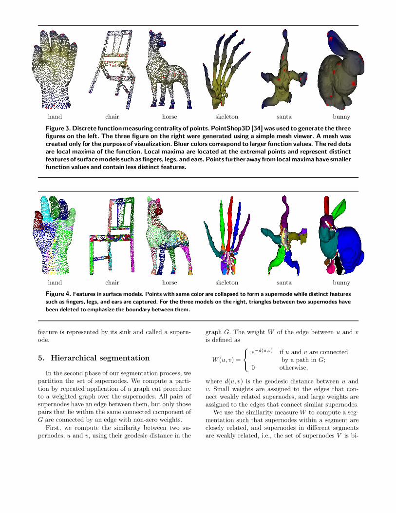
In our experiments, we use the value k = 7 to constructG. A higher value of k may be required if the pointsare embedded in a higher-dimensional space. Figure 1shows the construction of G, for k = 3. Figure 3 showsthe distribution of f for different surface models. Sinksof the discrete gradient flow field correspond to localmaxima of f and are marked in red. Figure 2 illustratesthe identification of features corresponding to the sinks,Figure 4 shows features extracted from various surfacemodels. Sinks and their associated points capture dis-tinct features like legs, fingers, ears, etc. Furthermore,the locations of sinks and features are invariant un-der rigid transformation of the input. Henceforth, each

hand chair horse skeleton santa bunny

Figure 3. Discrete functionmeasuring centrality of points. PointShop3D [34] was used to generate the threefigures on the left. The three figure on the right were generated using a simple mesh viewer. A mesh wascreated only for the purpose of visualization. Bluer colors correspond to larger function values. The red dotsare local maxima of the function. Local maxima are located at the extremal points and represent distinctfeatures of surfacemodels such as fingers, legs, and ears. Points further away from localmaxima have smallerfunction values and contain less distinct features.

hand chair horse skeleton santa bunny

Figure 4. Features in surface models. Points with same color are collapsed to form a supernode while distinct features

such as fingers, legs, and ears are captured. For the three models on the right, triangles between two supernodes have

been deleted to emphasize the boundary between them.

feature is represented by its sink and called a supern-ode.

5. Hierarchical segmentation

In the second phase of our segmentation process, wepartition the set of supernodes. We compute a parti-tion by repeated application of a graph cut procedureto a weighted graph over the supernodes. All pairs ofsupernodes have an edge between them, but only thosepairs that lie within the same connected component ofG are connected by an edge with non-zero weights.

First, we compute the similarity between two su-pernodes, u and v, using their geodesic distance in the

graph G. The weight W of the edge between u and vis defined as

W (u, v) =

e−d(u,v) if u and v are connectedby a path in G;

0 otherwise,

where d(u, v) is the geodesic distance between u andv. Small weights are assigned to the edges that con-nect weakly related supernodes, and large weights areassigned to the edges that connect similar supernodes.

We use the similarity measure W to compute a seg-mentation such that supernodes within a segment areclosely related, and supernodes in different segmentsare weakly related, i.e., the set of supernodes V is bi-

sected into two disjoint sets V1 and V2 such that thenormalized cut value

NCut(V1, V2) =cut(V1, V2)

assoc(V1, V )+

cut(V1, V2)assoc(V2, V )

,

is minimized. Here,

cut(V1, V2) =∑

v1∈V1,v2∈V2

W (v1, v2)

andassoc(V1, V ) =

∑v1∈V1,v∈V

W (v1, v).

Minimizing NCut maximizes the association within asegment while minimizing the cut between segments.Minimizing NCut also avoids bias toward small seg-ments, which are favored if the cut value is minimizedwithout normalization.

Discrete minimization of NCut is NP -complete. Shiand Malik introduced the idea of a normalized cut forimage segmentation and showed that an approximatesolution to the above minimization problem can be ob-tained by first solving the generalized eigenvalue sys-tem

(D − W )y = λy,

where D is a diagonal matrix, whose ith diagonal entrydii is the degree of vi ∈ V , i.e.,

dii =∑

v∈V \vi

W (vi, v),

and the eigenvector y corresponds to the second small-est eigenvalue [30]. They also proved that NCut(V1, V2)is minimized when

yi ={

a, vi ∈ V1

b, vi ∈ V2.

For a near-optimal bisection, all points vi that liewithin a cluster have approximately same value yi. Wedetermine the split value α that identifies the near-optimal cut from a set of uniformly spaced values be-tween the smallest and largest elements in the eigen-vector. Then, we form two clusters of vi that corre-spond to the near-optimal solution of the normalizedcut:

vi ∈{

V1 if yi < αV2 otherwise.

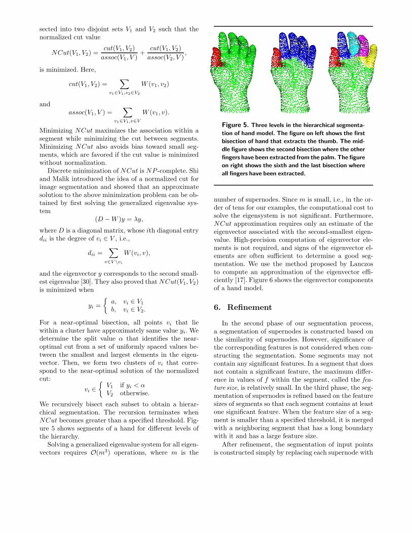
We recursively bisect each subset to obtain a hierar-chical segmentation. The recursion terminates whenNCut becomes greater than a specified threshold. Fig-ure 5 shows segments of a hand for different levels ofthe hierarchy.

Solving a generalized eigenvalue system for all eigen-vectors requires O(m3) operations, where m is the

Figure 5. Three levels in the hierarchical segmenta-

tion of hand model. The figure on left shows the first

bisection of hand that extracts the thumb. The mid-

dle figure shows the second bisection where the other

fingers have been extracted from the palm. The figure

on right shows the sixth and the last bisection where

all fingers have been extracted.

number of supernodes. Since m is small, i.e., in the or-der of tens for our examples, the computational cost tosolve the eigensystem is not significant. Furthermore,NCut approximation requires only an estimate of theeigenvector associated with the second-smallest eigen-value. High-precision computation of eigenvector ele-ments is not required, and signs of the eigenvector el-ements are often sufficient to determine a good seg-mentation. We use the method proposed by Lanczosto compute an approximation of the eigenvector effi-ciently [17]. Figure 6 shows the eigenvector componentsof a hand model.

6. Refinement

In the second phase of our segmentation process,a segmentation of supernodes is constructed based onthe similarity of supernodes. However, significance ofthe corresponding features is not considered when con-structing the segmentation. Some segments may notcontain any significant features. In a segment that doesnot contain a significant feature, the maximum differ-ence in values of f within the segment, called the fea-ture size, is relatively small. In the third phase, the seg-mentation of supernodes is refined based on the featuresizes of segments so that each segment contains at leastone significant feature. When the feature size of a seg-ment is smaller than a specified threshold, it is mergedwith a neighboring segment that has a long boundarywith it and has a large feature size.

After refinement, the segmentation of input pointsis constructed simply by replacing each supernode with

hand chair horse skeleton santa bunny

Figure 7. Segmentation of point-sampled surfaces.Distinct parts of a model such as fingers, legs, and ears are identified

without using an explicit surface representation.

1 2 3 4 5 6 7 8 9 10 11 12 13−1

−0.8

−0.6

−0.4

−0.2

0

0.2

0.4

1 2 3 4 5 6 7 8 9 10 11 12−0.3

−0.2

−0.1

0

0.1

0.2

0.3

0.4

Figure 6. Eigenvector analysis for hierarchical seg-

mentation of hand model. The green dots represent

the values of individual eigenvector components, and

the blue line indicates the split value used for bisec-

tion. The left graph shows the eigenvector for the first

bisection of the hand that segments out the thumb.

The right graph shows the eigenvector for the sec-

ond bisection that segments out the four fingers. All

eigenvectors are computed to a required precision us-

ing a single Lanczos iteration, and eigenvector compo-

nents have approximately piecewise constant values.

points that constitute its associated feature. Figure 7shows the results of our segmentation process.

7. Analysis and Optimization

In the following, we analyze storage costs andrun time complexity of our algorithms and de-scribe an approximation scheme that results in anorder-of-magnitude improvement in run time behav-ior.

Memory requirement is an issue when the input dataset is large. Our method uses Euclidean and geodesicdistances between points. However, only distances be-

tween certain points need to be stored during the con-struction of segmentation. For example, Euclidean dis-tances between near neighbors are used to computethe geodesic distances. Thus, the space requirement tostore Euclidean distances is Θ(kn), where n is the num-ber of input points, and k is the number of nearestneighbors considered for each point. Geodesic distancebetween two local maxima is used to compute similar-ity between the corresponding supernodes. Thus, onlythe geodesic distances between m local maxima needto be stored, resulting in Θ(m2) storage complexity.

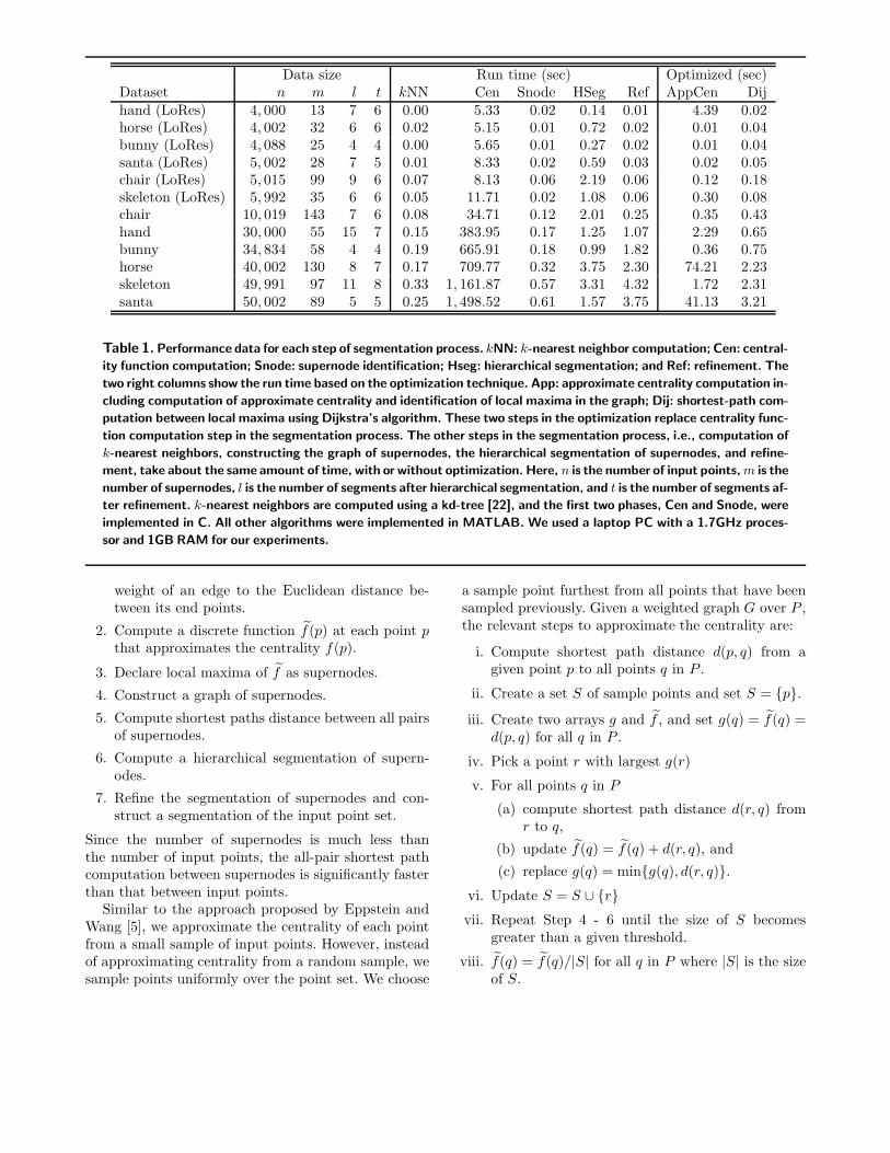
Table 1 summarizes our experimental results.Clearly, the geodesic distance computations re-quired to evaluate centrality is a computationalbottleneck. The computational complexities of the dif-ferent steps are:

k-nearest neighbor computation: O(kn log(n))Centrality function computation: O(n2 log(n))Feature identification: O(kn)Hierarchical segmentation: O(lm2)Refinement: O(l2).

Here, l is the number of segments resulting from thesecond phase. The number of Lanczos iterations re-quired to obtain a desired precision for the secondeigenvector is assumed to be independent of the in-put size.

It is possible to modify our segmentation process sothat the computational bottleneck in the geodesic dis-tance computation between all pairs of input pointscan be avoided while maintaining the quality of seg-mentation. This modification is based on the followingsteps:

1. Construct a weighted graph G over P whose edgesare given by the k-nearest neighbors. Set the

Data size Run time (sec) Optimized (sec)Dataset n m l t kNN Cen Snode HSeg Ref AppCen Dijhand (LoRes) 4, 000 13 7 6 0.00 5.33 0.02 0.14 0.01 4.39 0.02horse (LoRes) 4, 002 32 6 6 0.02 5.15 0.01 0.72 0.02 0.01 0.04bunny (LoRes) 4, 088 25 4 4 0.00 5.65 0.01 0.27 0.02 0.01 0.04santa (LoRes) 5, 002 28 7 5 0.01 8.33 0.02 0.59 0.03 0.02 0.05chair (LoRes) 5, 015 99 9 6 0.07 8.13 0.06 2.19 0.06 0.12 0.18skeleton (LoRes) 5, 992 35 6 6 0.05 11.71 0.02 1.08 0.06 0.30 0.08chair 10, 019 143 7 6 0.08 34.71 0.12 2.01 0.25 0.35 0.43hand 30, 000 55 15 7 0.15 383.95 0.17 1.25 1.07 2.29 0.65bunny 34, 834 58 4 4 0.19 665.91 0.18 0.99 1.82 0.36 0.75horse 40, 002 130 8 7 0.17 709.77 0.32 3.75 2.30 74.21 2.23skeleton 49, 991 97 11 8 0.33 1, 161.87 0.57 3.31 4.32 1.72 2.31santa 50, 002 89 5 5 0.25 1, 498.52 0.61 1.57 3.75 41.13 3.21

Table 1. Performance data for each step of segmentation process. kNN: k-nearest neighbor computation; Cen: central-

ity function computation; Snode: supernode identification; Hseg: hierarchical segmentation; and Ref: refinement. The

two right columns show the run time based on the optimization technique. App: approximate centrality computation in-

cluding computation of approximate centrality and identification of local maxima in the graph; Dij: shortest-path com-

putation between local maxima using Dijkstra’s algorithm. These two steps in the optimization replace centrality func-

tion computation step in the segmentation process. The other steps in the segmentation process, i.e., computation of

k-nearest neighbors, constructing the graph of supernodes, the hierarchical segmentation of supernodes, and refine-

ment, take about the same amount of time, with or without optimization. Here, n is the number of input points, m is the

number of supernodes, l is the number of segments after hierarchical segmentation, and t is the number of segments af-

ter refinement. k-nearest neighbors are computed using a kd-tree [22], and the first two phases, Cen and Snode, were

implemented in C. All other algorithms were implemented in MATLAB. We used a laptop PC with a 1.7GHz proces-

sor and 1GB RAM for our experiments.

weight of an edge to the Euclidean distance be-tween its end points.

2. Compute a discrete function f̃(p) at each point pthat approximates the centrality f(p).

3. Declare local maxima of f̃ as supernodes.

4. Construct a graph of supernodes.

5. Compute shortest paths distance between all pairsof supernodes.

6. Compute a hierarchical segmentation of supern-odes.

7. Refine the segmentation of supernodes and con-struct a segmentation of the input point set.

Since the number of supernodes is much less thanthe number of input points, the all-pair shortest pathcomputation between supernodes is significantly fasterthan that between input points.

Similar to the approach proposed by Eppstein andWang [5], we approximate the centrality of each pointfrom a small sample of input points. However, insteadof approximating centrality from a random sample, wesample points uniformly over the point set. We choose

a sample point furthest from all points that have beensampled previously. Given a weighted graph G over P ,the relevant steps to approximate the centrality are:

i. Compute shortest path distance d(p, q) from agiven point p to all points q in P .

ii. Create a set S of sample points and set S = {p}.iii. Create two arrays g and f̃ , and set g(q) = f̃(q) =

d(p, q) for all q in P .

iv. Pick a point r with largest g(r)

v. For all points q in P

(a) compute shortest path distance d(r, q) fromr to q,

(b) update f̃(q) = f̃(q) + d(r, q), and

(c) replace g(q) = min{g(q), d(r, q)}.vi. Update S = S ∪ {r}vii. Repeat Step 4 - 6 until the size of S becomes

greater than a given threshold.

viii. f̃(q) = f̃(q)/|S| for all q in P where |S| is the sizeof S.

After the completion of the above steps, f̃(p) contains avalue that is approximately equal to the centrality of p.We sample Θ(

√n) points, and therefore, the complex-

ity of computing approximate centrality of all pointsbecomes O(n

√n log(n)).

Figure 8 shows that the samples are uniformly dis-tributed over the input point sets and that the locationof the local maxima of f̃ are close to the location of lo-cal maxima of f . If centralities are normalized to havevalues between zero and one, the root mean squared er-rors are less than 0.08 for all point sets used in this pa-per. Figure 9 shows that there is no loss in the qualityof segmentation due to the approximation. The rightcolumns in Table 1 document the benefit of the op-timization. The run time is reduced by an order-of-magnitude.

skeleton santa bunny

skeleton santa bunny

Figure 8. Top: uniform distribution of sample points

(red) in input point sets (blue). Bottom: discrete func-

tion measuring approximate centrality. Blue regions

have larger function values. The uniform distribution

of sample points results in a good approximation of

centrality.Maximaof the function (marked in red) rep-

resent distinct features similar to maxima of the func-

tion shown in Figure 3.

8. Future Work

We have introduced a technique for partitioningpoint-sampled surfaces into distinct features withoutexplicit construction of a mesh. Since our methodworks directly with a point set, it can be extendedto segment point sets in high-dimensional and non-Euclidean spaces, where each point represents a fixed-length feature vector. Examples are collection of pro-tein shape analysis [26] and hand-written characterrecognition [31] represented as sets of points in high-dimensional space. Each dimension would correspondto a characteristic attribute of a protein or a hand-written character. We plan to extend our method toconstruct meaningful segmentations of such data sets.

hand chair horse

skeleton santa bunny

Figure9.Segmentationofpoint-sampled surfaces us-

ingapproximatecentrality.Distinctparts are identified

similarly to the results shown in Figure 7.

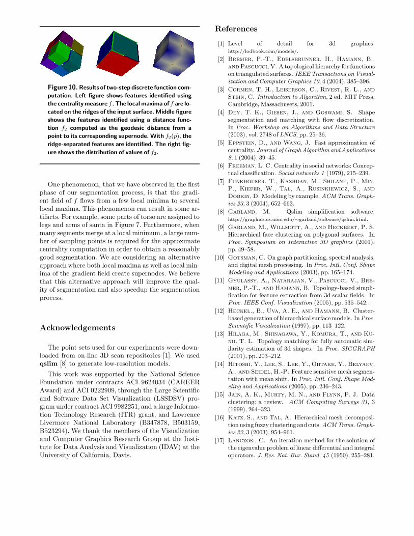
We are also considering an alternate approach tofeature identification, using a new function f2(p) thatmeasure the geodesic distance from p to its supernodewhich is the local maximum of f . This approach allowsus to identify ridge-separated features in a point sam-pled surface such as a laser scan of a cube shown inFigure 10.

Figure 10. Results of two-step discrete function com-

putation. Left figure shows features identified using

the centralitymeasure f . The local maxima of f are lo-

cated on the ridges of the input surface. Middle figure

shows the features identified using a distance func-

tion f2 computed as the geodesic distance from a

point to its corresponding supernode. With f2(p), the

ridge-separated features are identified. The right fig-

ure shows the distribution of values of f2.

One phenomenon, that we have observed in the firstphase of our segmentation process, is that the gradi-ent field of f flows from a few local minima to severallocal maxima. This phenomenon can result in some ar-tifacts. For example, some parts of torso are assigned tolegs and arms of santa in Figure 7. Furthermore, whenmany segments merge at a local minimum, a large num-ber of sampling points is required for the approximatecentrality computation in order to obtain a reasonablygood segmentation. We are considering an alternativeapproach where both local maxima as well as local min-ima of the gradient field create supernodes. We believethat this alternative approach will improve the qual-ity of segmentation and also speedup the segmentationprocess.

Acknowledgements

The point sets used for our experiments were down-loaded from on-line 3D scan repositories [1]. We usedqslim [8] to generate low-resolution models.

This work was supported by the National ScienceFoundation under contracts ACI 9624034 (CAREERAward) and ACI 0222909, through the Large Scientificand Software Data Set Visualization (LSSDSV) pro-gram under contract ACI 9982251, and a large Informa-tion Technology Research (ITR) grant, and LawrenceLivermore National Laboratory (B347878, B503159,B523294). We thank the members of the Visualizationand Computer Graphics Research Group at the Insti-tute for Data Analysis and Visualization (IDAV) at theUniversity of California, Davis.

References

[1] Level of detail for 3d graphics.http://lodbook.com/models/.

[2] Bremer, P.-T., Edelsbrunner, H., Hamann, B.,

and Pascucci, V. A topological hierarchy for functionson triangulated surfaces. IEEE Transactions on Visual-ization and Computer Graphics 10, 4 (2004), 385–396.

[3] Cormen, T. H., Leiserson, C., Rivest, R. L., and

Stein, C. Introduction to Algorithm, 2 ed. MIT Press,Cambridge, Massachusets, 2001.

[4] Dey, T. K., Giesen, J., and Goswami, S. Shapesegmentation and matching with flow discretization.In Proc. Workshop on Algorithms and Data Structure(2003), vol. 2748 of LNCS, pp. 25–36.

[5] Eppstein, D., and Wang, J. Fast approximation ofcentrality. Journal of Graph Algorithm and Applications8, 1 (2004), 39–45.

[6] Freeman, L. C. Centrality in social networks: Concep-tual classification. Social networks 1 (1979), 215–239.

[7] Funkhouser, T., Kazhdan, M., Shilane, P., Min,

P., Kiefer, W., Tal, A., Rusinkiewicz, S., and

Dobkin, D. Modeling by example. ACM Trans. Graph-ics 23, 3 (2004), 652–663.

[8] Garland, M. Qslim simplification software.http://graphics.cs.uiuc.edu/∼garland/software/qslim.html.

[9] Garland, M., Willmott, A., and Heckbert, P. S.

Hierarchical face clustering on polygonal surfaces. InProc. Symposium on Interactive 3D graphics (2001),pp. 49–58.

[10] Gotsman, C. On graph partitioning, spectral analysis,and digital mesh processing. In Proc. Intl. Conf. ShapeModeling and Applications (2003), pp. 165–174.

[11] Gyulassy, A., Natarajan, V., Pascucci, V., Bre-

mer, P.-T., and Hamann, B. Topology-based simpli-fication for feature extraction from 3d scalar fields. InProc. IEEE Conf. Visualization (2005), pp. 535–542.

[12] Heckel., B., Uva, A. E., and Hamann, B. Cluster-based generation of hierarchical surfacemodels. InProc.Scientific Visualization (1997), pp. 113–122.

[13] Hilaga, M., Shinagawa, Y., Komura, T., and Ku-

nii, T. L. Topology matching for fully automatic sim-ilarity estimation of 3d shapes. In Proc. SIGGRAPH(2001), pp. 203–212.

[14] Hitoshi, Y., Lee, S., Lee, Y., Ohtake, Y., Belyaev,

A., and Seidel, H.-P. Feature sensitive mesh segmen-tation with mean shift. In Proc. Intl. Conf. Shape Mod-eling and Applications (2005), pp. 236–243.

[15] Jain, A. K., Murty, M. N., and Flynn, P. J. Dataclustering: a review. ACM Computing Surveys 31, 3(1999), 264–323.

[16] Katz, S., and Tal, A. Hierarchical mesh decomposi-tionusing fuzzy clusteringand cuts. ACMTrans.Graph-ics 22, 3 (2003), 954–961.

[17] Lanczos., C. An iteration method for the solution ofthe eigenvalue problem of linear differential and integraloperators. J. Res. Nat. Bur. Stand. 45 (1950), 255–281.

[18] Liu, R., and Zhang, H. Segmentation of 3d meshesthrough spectral clustering. In Proc. Pacific Graphics(2004), pp. 298–305.

[19] Mangan, A. P., and Whitaker, R. T. Partition-ing 3d surface meshes using watershed segmentation.IEEE Trans. Visualization and Computer Graphics 5,4 (1999), 308–321.

[20] Matsumoto, Y. An Introduction to Morse Theory.Amer. Math. Soc., 2002. Translated from Japanese byK. Hudson and M. Saito.

[21] Milnor., J. Morse Theory. Princeton Univ.Press, NewJersey, 1963.

[22] Mount, D. M., and Arya., S. Ann: A li-brary for approximate nearest neighbor searching.http://www.cs.umd.edu/∼mount/ANN/.

[23] Natarajan, V., and Pascucci, V. Volumetric dataanalysis using Morse-Smale complexes. In Proc. Intl.Conf. Shape Modeling and Applications (2005), pp. 320–325.

[24] Page, D. L., Koschan, A., and Abidi, M. A.

Perception-based 3d triangle mesh segmentation usingfast marching watersheds. In Proc. IEEE Conf. Com-puter Vision and Pattern Recognition (2003), vol. 2,pp. 27–32.

[25] Pauly, M., Keiser, R., Kobbelt, L. P., and Gross,

M. Shapemodelingwithpoint-sampledgeometry. ACMTransactions on Graphics (2003), 641–650.

[26] Roger, P., and Bohr., H. A new family of global pro-tein shape descriptors. ACM Computing Surveys 182(2003), 167–181.

[27] Schloegel, K., Karypis, G., and Kumar, V. CRPCParallel Computing Handbook. Morgan Kaufmann,2000, ch. Graph partitioning for High performance sci-entific simulations.

[28] Shalfman, S., Tal, A., and Katz, S. Metamorpho-sis of polyhedral surfaces using decomposition. In Proc.Eurographics (2002), pp. 219–228.

[29] Shamir, A. A formulation of boundary mesh segmen-tation. In Proc. Second International Symposium on3DPVT (2004), pp. 82–89.

[30] Shi, J., and Malik., J. Normalized cuts and image seg-mentation. IEEE Transactions on Pattern Analysis andMachine Intelligence 22 (2000), 888–905.

[31] Tenebaum, J. B., de Silva,V., andLangford., J. C.

A global geometric framework for nonlinear dimension-ality reduction. Science 190, 5500 (2000), 2319–2323.

[32] Wu, K., and Levine, M. D. 3d part segmentationusing simulated electrical charge distributions. IEEETrans. Pattern Analysis and Machine Intelligence 19,11 (1997), 1223–1235.

[33] Zhang, E., Mischaikow, K., and Turk, G. Feature-based surface parameterization and texture mapping.ACM Transactions on Graphics 24, 1 (2005), 1–27.

[34] Zwicker, M., Pauly, M., Knoll, O., and Gross, M.

Pointshop3d:An interactive system forpoint-based sur-face editing. In SIGGRAPH (2002), pp. 322–329.