Seismic data interpolation using a fast generalized ...mostafan/Files/Papers/fgft_GEO2011.pdf ·...

Seismic data interpolation using a fast generalized Fouriertransform

Mostafa Naghizadeh and Kristopher A. Innanen

ABSTRACT

We propose a fast and efficient method for interpolation of nonstationary seismic data.The proposed method utilizes fast generalized Fourier transform (FGFT) to identifythe space-wavenumber evolution of nonstationary spatial signals at each temporal fre-quency. The non-redundant nature of FGFT renders a big computational advantageto the proposed interpolation method. Next, a least-squares fitting scheme is used toretrieve the optimal FGFT coefficients representative of the ideal interpolated data.For randomly sampled data on a regular grid we seek a sparse representation of FGFTcoefficients in order to retrieve the missing samples. Also, to interpolate the regu-larly sampled seismic data at a given frequency, we use a mask function derived fromthe FGFT coefficients of the low frequencies. Synthetic and real data examples areprovided to examine the performance of the proposed method.

INTRODUCTION

The problems of seismic data reconstruction and interpolation have attained a specialstature in the seismic data processing community in recent years. Reconstruction methodsuse available seismic traces, measured on irregular and/or coarsely sampled grids in space,to estimate data on a regularly and sufficiently sampled grid. An effective solution can openthe door to application of multidimensional wave equation imaging and de-multiple algo-rithms to a data set, without having had to acquire it with the completeness these methodsdemand. In a useful method of interpolation/reconstruction we look for speed, stability inthe presence of noise and aliasing, and ability to manage complex events. In this paper wepropose an interpolation/reconstruction methodology which provides a constructive mix-ture of the above properties, and is also a theoretically sound framework within which tocarry out a range of wave based data analysis tasks.

Reconstruction methods can be divided into two main classes: wave equation based andsignal processing based. Most methods in the latter category, including the one we describein this paper, utilize transform domains such as Fourier (Duijndam et al., 1999; Liu, 2004;Abma and Kabir, 2005; Zwartjes and Gisolf, 2006), Radon (Darche, 1990; Trad et al., 2002),and curvelet (Hennenfent and Herrmann, 2008). A key issue in judging the performanceof transform-based reconstruction methods and their management of complex events lies intheir response to data nonstationarity.

In seismic data processing, nonstationarity means the frequency/wavenumber content ofthe signal varies in time/space. For instance, an absorptive medium causes nonstationarityin the time dimension by making the frequency content of a seismic pulse a function of pathlength. Also, seismic sections which contain hyperbolic and parabolic (or any nonlinear)

Fast generalized Fourier transform

2 FGFT interpolation

events produce nonstationary spatial signals in the f-x domain at a given frequency. Inter-polation/reconstruction methods typically cope with nonstationary signals through spatialwindowing. Inside sufficiently small spatial windows nonlinear seismic events appear linearor stationary. Hence, methods which assume stationarity such as those referenced above maybe applied. Naghizadeh and Sacchi (2009) have proposed an alternative method providinga beyond-alias interpolation of nonstationary seismic data. It is essentially a modificationof the f-x interpolation of Spitz (1991). In their method the windowing of the spatial axis isavoided through use of adaptive prediction filters. Although spatial windowing of data andthe adaptive f-x interpolation method are capable of handling nonstationarity, they lead tocomputationally demanding algorithms.

On another note, there exists a range of transformations specifically designed to dealwith identification and analysis of nonstationary behavior in signals that might be used asa basis for interpolation. The Gabor transform, for instance, is a class of short-time Fouriertransforms that has been used for a range of processing tasks such as nonstationary decon-volution (Margrave et al., 2003). Wavelet (Beylkin et al., 1991), curvelet (Candes et al.,2005; Candes and Donoho, 2004), and S-transform, are further examples. The S-transform(Stockwell et al., 1996) is a type of short-time Fourier transform in which the window sizeis frequency dependent. Larger windows are used for lower frequencies and smaller win-dows are used for higher frequencies. Consequently, the spectrum at a given frequencyis estimated with a number of samples appropriate to that frequency. Two properties ofthe aforementioned transforms work against their potential as a base for an interpolationmethod. They are redundant (the size of the transformed data set is larger than that of theoriginal data set) and computationally demanding. Hence, when applied to already largeseismic data volumes, they can cause unwanted data expansion. These transforms also sharethe computational issues associated with windowing/adaptive methods, and therefore, ontheir own, do not constitute a viable avenue to respond to them.

However, recent work on the S-transform has led to a fast, non-redundant algorithm(Brown et al., 2010), renewing the possibility of developing an efficient and effective inter-polation/reconstruction approach based on S-transform theory. In this paper, we developsuch an approach and examine its behavior when applied to synthetic and field data sets.First, because the transform algorithm is new, we will describe a straightforward and in-tuitive frequency domain computation of the fast generalized Fourier transform (FGFT).We will then combine FGFT with a least-squares fitting principle to formulate our FGFTInterpolation method. Synthetic and field data examples are examined.

BACKGROUND THEORY

Generalized Fourier transform

The S-transform of a time signal g(t) is defined as follows (Stockwell et al., 1996):

S(τ, f) =

∫ ∞−∞

g(t)|f |√2πe−

(τ−t)2f22 e−i2πftdt, (1)

where τ and f are the time and frequency coordinates, respectively. The term |f |√2πe−

(τ−t)2f22

is a Gaussian window which depends on time lag and frequency. The width of the Gaussian



window decreases with increasing frequency. This results in finer frequency resolution forlow frequencies and finer time resolution for high frequencies. If the window function isset to unity, equation 1 reverts to the ordinary Fourier transform. The S-transform can begeneralized by replacing the Gaussian window with other functions, such as Gabor and B-Spline windows. Brown et al. (2010) have used the term ”general Fourier-family transform”to refer to this entire group.

Equation 1 is a formula for calculation of the S-transform of an input signal g(t) inthe time domain. The same calculation can be carried out in the frequency domain. Infact, the S-transform in the Fourier domain turns out to be simpler to derive and easier toimplement than its time domain counterpart. Also, the frequency domain implementationof S-transform provides a framework for the FGFT method. The equivalence of the timeand frequency domain S-transforms, as well as the derivation of the method and algorithmdetails, are presented by Brown et al. (2010). Since this work is outside of typical geophysicalliterature, we begin with a brief overview of the frequency-domain S-transform algorithm,exemplifying it with the chirp function illustrated in Figure 1a.

The procedure of S-transform in the frequency domain is as follows

1. Transform g(t) to the Fourier domain to obtain G(f). Figures 1a and 1b show theoriginal chirp function and its Fourier domain representation, respectively.

2. Create a data matrix, G(f, f ′), using repeated instances of G(f), each time shiftingits elements (Figure 1c). This matrix is referred to as the data in the α-domain, wheref ′ represents the frequency shift. To be specific, the column of data at frequency shiftzero is the original Fourier domain representation of the data in Figure 1b. The othercolumns are shifted copies of Figure 1b.

3. Create a window matrix, W (f, f ′), the same size as the α-domain representation ofthe data (Figure 1d). The window function can be any symmetric smooth functionsuch as Gaussian, Hanning, B-spline, etc. The size of windows grows linearly fromlower to higher frequencies. The windows are chosen to be wider for high frequenciesand narrower for low frequencies to gain proper resolution in time-frequency analysis(Brown et al., 2010).

4. Multiply G(f, f ′) and W (f, f ′) element by element to window the data in the α-domain, obtaining G′(f, f ′) (Figure 1e).

5. Apply a 1D inverse Fourier transform along each row (i.e., the f ′ axis) of G′(f, f ′) toobtain the S-Transform of the original data (Figure 1f).

The chirp function in Figure 1a has more low frequency content at the start of the timesignal and more high frequency content at the end. The S-transform of the chirp function inFigure 1f reflects this evolution with local spectra trending toward high frequency as timeincreases.

A natural outcome of deploying wider/narrower windows in the frequency-domain toestimate high/low frequencies is a decreased/increased resolution at correspondent frequen-cies. This is illustrated in Figure 2, in which we apply the S-transform to a time signalcomposed of two stationary harmonics. Figures 2a and b show a time series composed of the



a)

0 100 200Time samples

-1

0

1

Am

plitu

de

c)-0.4

-0.2

0

0.2

0.4Nor

mal

ized

freq

uenc

y

-0.4 -0.2 0 0.2 0.4Frequency shift

e)-0.4

-0.2

0

0.2

0.4Nor

mal

ized

freq

uenc

y


b)

-0.4 -0.2 0 0.2 0.4Normalized frequency

0.1

0.5

0.9

Am

plitu

ded)

-0.4

-0.2

0

0.2

0.4Nor

mal

ized

freq

uenc

y-0.4 -0.2 0 0.2 0.4

Frequency shift

f)-0.4

-0.2

0

0.2

0.4Nor

mal

ized

freq

uenc

y

50 100 150 200 250Time samples

Figure 1: Frequency domain implementing of S-Transform. a) Original chirp function. b) Fouriertransform of (a). c) α-domain matrix built by shifting spectrum in (b). d) Window function withthe same size as the α-domain representation of the data in (c). e) Windowed α-domain obtainedby element by element multiplication of (c) and (d). f) S-transform of data obtained by applyinginverse Fourier transform on each row of (e).



sum of two sinusoids, and its amplitude spectrum, respectively. This signal is transformedto the α-domain (Figure 2c), in which a window function is designed (Figure 2d) and ap-plied to the α-domain signal (Figure 2e). The S-transform of the signal, shown in Figure2f, clearly represents the two harmonics, constant with respect to time. However, the lowfrequency harmonic is more highly resolved in the S-transform domain (narrow line) thanthe high frequency harmonic (wider line). This is an intrinsic property of the S-Transformthat can be utilized to build a faster transform algorithm, which we will discuss next.

Fast generalized Fourier transform (FGFT)

The frequency-dependence of the resolution of the S-transform suggests that computationalefficiency can be increased by adopting sampling criteria varying from high to low fre-quency. Brown et al. (2010) used a dyadic segmentation approach, through which highfrequencies (which are inherently low resolution) are coarsely sampled and low frequencies(which are inherently high resolution) are finely sampled in the α-domain. Figure 3a illus-trates the dyadic segmentation of the α-domain. The domain is subdivided into squares(solid lines) centered around zero frequency-shift. The squares are larger for high frequen-cies and smaller for low frequencies. Within each segment, the center frequency (dashedline) is representative of all the segment’s frequencies. The S-transform of the data is thenobtained by applying inverse Fourier transform on the data in the dashed lines only. Thisnew segmentation consequently leads to significantly increased efficiency, compared to thefull S-transform. The cost is that the inverse Fourier transform on the center frequency(dashed lines) must meaningfully represent the signal’s behavior over all the frequencies,in a given square segment of the data. Brown et al. (2010) called this transform as Fastgeneralized Fourier transform (FGFT). Notice that it is also possible to use other optionalforms of segmentation instead of dyadic segmentation.

To finalize the form of the FGFT algorithm, recall that the α-domain was a shiftedmatrix version of the Fourier transform of the time signal. Unshifting the dashed linesillustrated in Figure 3a recovers their respective locations on the frequency axis (Figure3b). This implies that the S-transform is equivalent to the application of inverse Fouriertransforms, over windows of varying size on the original signal in the Fourier domain. Wemust then apply short windows at low frequencies and large windows at high frequencies.The dyadic segmentation achieves this optimal segmentation non-redundantly in the Fourierdomain. If we imagine dropping each dashed line segment to zero normalized frequency, wesee that the vector of utilized data exactly reproduces the original frequency vector. Thisis the framework for the FGFT algorithm.

Figure 4 illustrates schematically an application of the FGFT algorithm. Figure 4arepresents a time signal containing 16 samples. A fast Fourier transform is applied to thetime signal to obtain the frequency domain representation illustrated in Figure 4b. Inthe frequency domain the signal is dyadically segmented (dashed boxes), and within eachsegment inverse Fourier transforms are applied to the data. The segmentation of Fourierdomain into smaller windows follows the rationale that is explained in Figure 3. In thisarticle, we perform the segmentation with the window sizes which are growing by power of2. However, depending on the application, one can deploy other forms of segmentation. It isalso important to mention that each segment needs to be properly tapered on the edges usinga tapering window, for instance Gaussian window, to avoid the ringing effects of the Fourier



a)

0 100 200Time samples

-2

-1

0

1

2

Am

plitu

de

c)-0.4

-0.2

0

0.2

0.4Nor

mal

ized

freq

uenc

y


e)-0.4

-0.2

0

0.2

0.4Nor

mal

ized

freq

uenc

y


b)

-0.4 -0.2 0 0.2 0.4Normalized frequency

0.1

0.5

0.9

Am

plitu

ded)

-0.4

-0.2

0

0.2

0.4Nor

mal

ized

freq

uenc

y-0.4 -0.2 0 0.2 0.4

Frequency shift

f)-0.4

-0.2

0

0.2

0.4Nor

mal

ized

freq

uenc

y

50 100 150 200 250Time samples

Figure 2: S-Transform of a signal composed of two sine functions. a) Original function. b) Fouriertransform of (a). c) α-domain matrix built by shifting spectrum in (b). d) Window function withthe same size as the α-domain representation of the data in (c). e) Windowed α-domain obtainedby element by element multiplication of (c) and (d). f) S-transform of data obtained by applyinginverse Fourier transform on each row of (e).



0

-0.25

-0.5

0.25

0.5

-0.5 -0.25 0 0.25 0.5Frequency shift

Nor

mal

ized

freq

uenc

ya)

0

-0.25

-0.5

0.25

0.5

-0.5 -0.25 0 0.25 0.5Frequency shift

Nor

mal

ized

freq

uenc

y

b)

Figure 3: a) Dyadic segmentation of α-domain. b) Unshifted dyadic segments. If each dashed linesegment in (b) is dropped to zero normalized frequency, the data exactly reproduces the originalfrequency vector of data.

transform. Notice that smaller windows are used for low frequencies and larger windowsfor high frequencies. The output is illustrated in Figure 4c. Each individual inverse Fouriertransform is represented by a particular symbol in Figure 4c (square, diamond, triangle,circle). Assuming a real time signal, we expect a symmetric outcome. So we may then focusour attention on the right hand side of the output, indicated with an underbrace.

Next, to properly represent the time-frequency behavior of the data, the underbracedFGFT coefficients must be arrayed in a 2D plot. Figure 4d illustrates this arrangement ofFGFT coefficients. Each individual element of a given inverse Fourier transform is distin-guished from the others in that group via size. Hence each FGFT coefficient is uniquelyrepresented by a symbol type and size. Figure 4d illustrates how these outputs are dis-tributed. We note that there is better time resolution in the high frequencies and betterfrequency resolution in the low frequencies. The inverse or adjoint FGFT is performed byreversing the order of operations from Figures 4a-c, by replacing inverse Fourier transformswith Fourier transforms and vice versa. The algorithms for both forward and adjoint FGFTare described by Brown et al. (2010).

Figure 5a shows the same chirp function illustrated in Figure 1a. Figure 5b showsthe FGFT of Figure 5a. Figure 5c illustrates the 2D array of FGFT coefficients afterproper up-scaling, i.e., the time-frequency decomposition of the chirp. Because the originalchirp input is real, we only include the positive frequencies for this example. The FGFTevidently captures the nonstationary nature of the chirp function. The low frequenciespredominate at the beginning of the signal and high frequencies predominate at the end.Figure 5d illustrates the adjoint FGFT acting on the FGFT coefficients of the chirp function.The adjoint FGFT recovers the original data within a small error level produced by thewindowing step.

The undesirable windowing error and the desirable time-frequency sensitivity of the



Time samples1 16a)

Normalized frequency-0.5 0.0 0.5

b)

FGFT samplesc)

Time samples1 160.0

0.5

Nor

mal

ized

freq

uenc

y

d)

Figure 4: Graphical representation of implementing FGFT. a) Original signal with 16 time samples.b) Fourier transform of original data in (a). c) FGFT representation of data after applying inverseFourier transform on each dashed box of data in (b). d) The time-frequency interpretation of FGFTcoefficients in (c) only for positive frequencies.



a)

0 50 100 150 200 250Time samples

-1

0

1

Am

plitu

de

b)

50 100 150 200 250FGFT samples

50

100

150

Am

plitu

de

c)

0.1

0.2

0.3

0.4

Nor

mal

ized

freq

uenc

y

50 100 150 200 250Time samples

d)

0 50 100 150 200 250Time samples

-1

0

1

Am

plitu

de

Figure 5: a) Original chirp signal. b) The FGFT coefficients of (a). c) 2D plot of FGFT coefficientsclearly showing the time-frequency distribution of chirp signal. d) The recovered chirp signal byapplying inverse FGFT on (b).



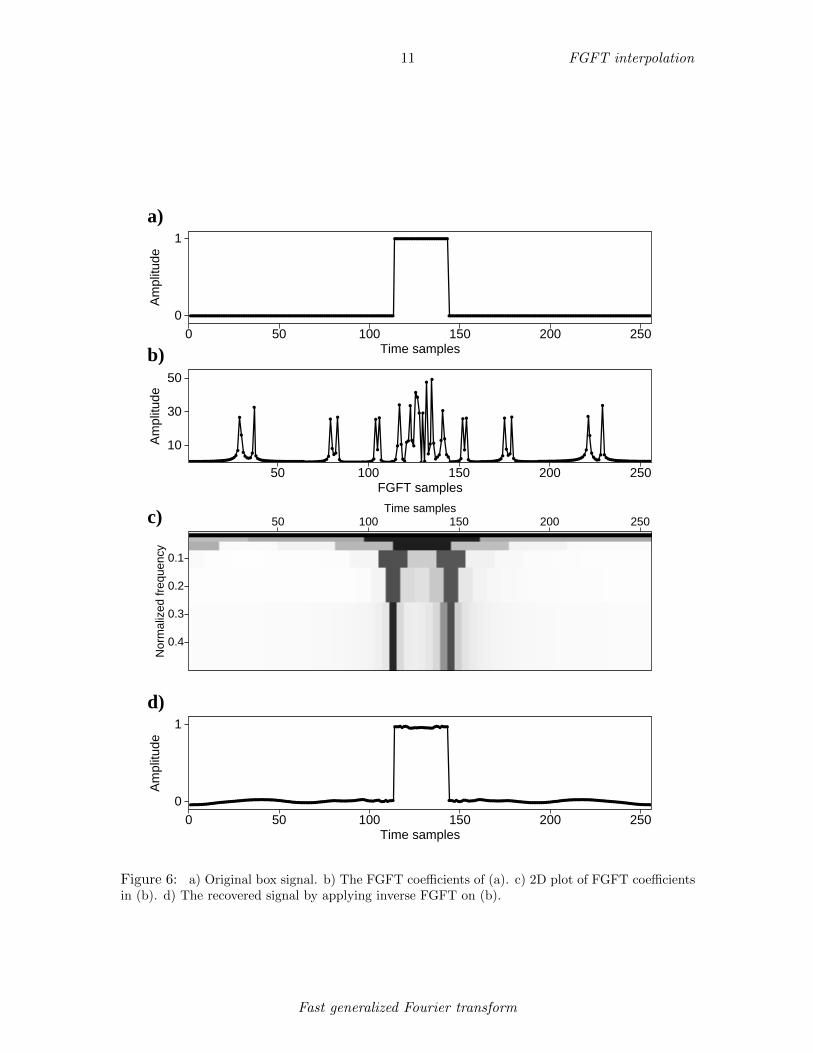
FGFT are more pronounced in a signal with sharp discontinuities. For example, Figure 6aillustrates a box function, which contains two regions of relatively dramatic nonstationarybehavior. Figures 6b and 6c illustrate the FGFT coefficients and their 2D time-frequencyinterpretation, respectively. The FGFT coefficients have successfully identified the locationof the box function in the time axis. Figure 6d shows the result of applying adjoint FGFTon the coefficients of FGFT.

FGFT INTERPOLATION OF SEISMIC DATA

We now turn our attention to the problem of reconstructing seismic data. We represent thedesired regularly sampled nonstationary signal of length N as d = (d1, d2, . . . , dN )T . Nextwe assume that we only have M out of N samples available, and that the remaining N −Msamples are missing. We represent the available samples as dobs. The desired signal d andobserved samples dobs are related by a sampling matrix T (Liu, 2004), through:

dobs = Td . (2)

We investigate the structure of sampling matrix T using a simple example. Assumethat the desired signal d has 5 samples but only 3, say {d2, d4, d5}, are available. Equation2 can be written as d2

d4d5

=

0 1 0 0 00 0 0 1 00 0 0 0 1

d1d2d3d4d5

. (3)

The transpose of the sampling matrix, TT , correctly places the available samples in theoutput and puts zeros in the samples corresponding to missing data.

The interpolation problem is under-determined and hence to solve it we require someprior information. To provide this, let us consider the FGFT coefficients g of the desired,fully sampled signal. These must be related to d by

g = Gd , (4)

where G represents the forward FGFT operator. The adjoint FGFT operator GT canfurthermore be used to express the desired interpolated data d in terms of g as follows

d ≈ GT Wg , (5)

where we have introduced a diagonal weight function W that preserves a subset of FGFTcoefficients. Inserting equation 5 into 2 yields

dobs ≈ TGT Wg . (6)

Let us assume for the moment that the operator W is known. The system of equationsin equation 6 is under-determined (Menke, 1989) and therefore, it admits an infinite number



a)

0 50 100 150 200 250Time samples

0

1

Am

plitu

de

b)

50 100 150 200 250FGFT samples

10

30

50

Am

plitu

de

c)

0.1

0.2

0.3

0.4

Nor

mal

ized

freq

uenc

y

50 100 150 200 250Time samples

d)

0 50 100 150 200 250Time samples

0

1

Am

plitu

de

Figure 6: a) Original box signal. b) The FGFT coefficients of (a). c) 2D plot of FGFT coefficientsin (b). d) The recovered signal by applying inverse FGFT on (b).



of solutions. A stable and unique solution can be found by minimizing the following costfunction (Tikhonov and Goncharsky, 1987)

J = ||dobs −TGTWg||22 + µ2||g||22 , (7)

where µ is the trade-off parameter. We minimize the cost function J using the method ofconjugate gradients (Hestenes and Stiefel, 1952). The conjugate gradients method does notrequire the explicit knowledge of G in matrix form. It requires the action of operators GT

and G on a vector in the coefficient and data spaces, respectively (Claerbout, 1992). Thegoal of the proposed algorithm is to find the coefficients g that minimize J , and use themto reconstruct the data via the adjoint FGFT operator d = GT g.

Derivation of the weight function W

The weight function plays an important role in the FGFT interpolation method. An optimaldesign for the weight function will depend on the form of the sampling function T.

Case 1: Randomly missing samples on a regular grid

For a randomly sampled signal one can impose a sparsity constraint to the FGFT coeffi-cients. This corresponds to a weight function which diminishes small amplitude coefficientsand preserves large ones (Sacchi et al., 1998). The large FGFT coefficients correspond withcoherent features in a data set. By suppressing the small FGFT coefficients, the coherentdata features will be reintroduced across regions where data was initially missing.

We adapt an Iteratively Re-weighted Least Squares (Scales and Gersztenkorn, 1988)approach to achieve this purpose. The algorithm is summarized as follow

Initialization W0 = IFor k = 1, 2, 3 . . .gk = argmin

g{||dobs −TGTWk−1g||22 + µ2||g||22}

Wk = diag(abs(gk))End

(8)

where diag(abs(.)) builds a diagonal matrix from the absolute values of a vector. The weightfunction was initiated with an identity matrix and was updated by the absolute value ofFGFT coefficients after each least-squares fitting. The updating step of IRLS method servesto amplify the high amplitude FGFT coefficients and eliminate the low amplitude ones. Ourtests show that using a small number of internal iteration for conjugate gradients (3 or 4)and more iterations of external re-weighting, produces optimal results. Using more internaliterations for conjugate gradients could lead to spurious high frequency features.

Case 2: Regularly missing samples

For a signal with regularly missing samples (zeros in the location of missing samples),a different strategy is needed. Regular sampling leaves large amplitude artifacts in any



Fourier domain representation of data (Naghizadeh and Sacchi, 2010). In the S-transformdomain, the high amplitude artifacts appear in high frequencies at all times. This meansthat a sparse constraint in the S-transform domain will tend to poorly interpolate the highfrequencies (such artifacts may also appear, though generally to a lesser extent, in randomsampling cases). In order to avoid this pitfall and correctly interpolate regularly missingsamples using the FGFT framework, we must be able to predict the location of desirablevs. undesirable coefficients. The weight function can then be a simple mask function whichhas the value of 1 for the coefficients in the desirable locations and zero elsewhere. For1D signals, making such a prediction would be difficult, likely impossible. However, formultidimensional seismic data one can use the half frequency of the original data to obtainproper weight function for a desired frequency in the interpolated data (Spitz, 1991). Wewill pursue this further in the numerical examples to follow.

EXAMPLES

1D chirp function

Randomly missing samples

We begin by applying FGFT interpolation on a 1D chirp function. Figure 7a shows the orig-inal chirp function, illustrated in Figure 5a, after randomly eliminating 50% of its samples.Figure 7b depicts the FGFT domain representation of the signal in Figure 7a. Comparisonof the FGFT of the original chirp function (Figure 5b) with the FGFT of the randomly dec-imated chirp function (Figure 7b) illustrates the introduction of high amplitude artifacts,especially in the high frequencies. Figure 7c shows the FGFT of reconstructed data afterapplying equation 8. The reconstructed chirp function in Figure 7d is obtained by applyinginverse FGFT to the recovered coefficients in Figure 7c. Notice that the reconstruction al-gorithm has been able to recover the nonstationary signature of the original chirp function.

Regularly missing samples

Next, we examine the performance of FGFT interpolation on a regularly decimated versionof the same chirp function. Figure 8a illustrates the regularly decimated input. Figure8b illustrates the FGFT domain representation of the data in Figure 8a. The regulardecimation of the chirp function has created a series of high amplitude artifacts in all of thetime samples in the high frequency range. Figure 8c illustrates the data in the FGFT domainafter applying an un-modified version of equation 8. The sparsity constraint imposed byEquation 8 has evidently retained undesirable time sample locations at high frequencies.Figure 8d shows the reconstructed chirp function after applying an inverse FGFT to therecovered coefficients in Figure 8c.

Since this is a 1D signal, we would normally be unable to interpolate the data withoutknowing in advance what the original signal was. Let us nevertheless demonstrate theimprovement that a well-designed mask can have on the results in Figure 8. We createthe mask function, pictured in Figure 9a, using the FGFT domain representation of theoriginal, fully sampled, chirp function in Figure 5b. We give the mask value of one to the



a)

0 50 100 150 200 250-1

0

1

Am

plitu

de

b)

0.1

0.2

0.3

0.4

Nor

mal

ized

freq

uenc

y

50 100 150 200 250

c)

0.1

0.2

0.3

0.4

Nor

mal

ized

freq

uenc

y

50 100 150 200 250

d)

0 50 100 150 200 250Time samples

-1

0

1

Am

plitu

de

Figure 7: a) Randomly sampled chirp function by randomly replacing 50% of original chirp functionin Figure 5a with zeros. b) 2D plot of FGFT coefficients of (a). c) Retrieved FGFT coefficient usingalgorithm 8. d) The reconstructed chirp signal using the FGFT interpolation.



a)

0 50 100 150 200 250-1

0

1

Am

plitu

de

b)

0.1

0.2

0.3

0.4

Nor

mal

ized

freq

uenc

y

50 100 150 200 250

c)

0.1

0.2

0.3

0.4

Nor

mal

ized

freq

uenc

y

50 100 150 200 250

d)

0 50 100 150 200 250Time samples

-1

0

1

Am

plitu

de

Figure 8: a) Regularly decimated chirp function by replacing odd number samples of originalchirp function in Figure 5a with zeros. b) 2D plot of FGFT coefficients of (a). c) Retrieved FGFTcoefficient using algorithm 8. Reconstructed chirp function by applying inverse FGFT to (c).



25% highest FGFT amplitudes and set the remaining 75% to zero. This mask functionis used in equation 7 to retrieve the FGFT coefficients in Figure 9b. The reconstructedchirp function is shown in Figure 9c. Evidently, in the presence of a priori informationpointing us preferentially to certain regions of the FGFT domain, we may expect dramaticimprovement in interpolation of a regularly decimated signal.

Synthetic seismic data

Randomly missing samples

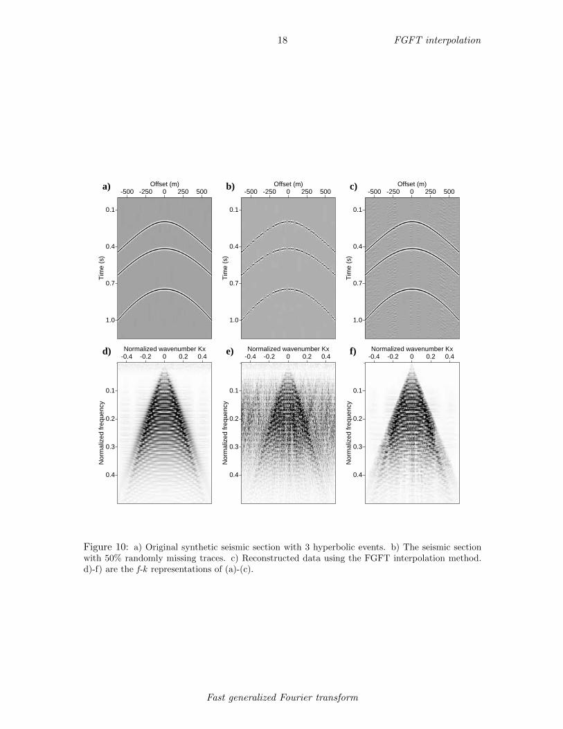
For randomly sampled seismic sections each frequency can be reconstructed independently.This is because random sampling creates low amplitude artifacts in the Fourier domainwhich can be eliminated by sparsity constraints. The amplification of high values anddiminishment of low values in the frequency domain occurs within equation 8. Figure 10ashows an original synthetic seismic section with three hyperbolic events composed of 202traces. Figure 10b shows the section of missing data after randomly eliminating 50% of thetraces. Figure 10c shows the FGFT reconstructed data after applying Equation 8 for eachsingle frequency. Notice that the non-redundant nature of FGFT interpolation create smallamplitude artifacts in the interpolated data. This means there is a trade-off between theresolution and speed of the interpolation method. Figures 10d, 10e, and 10f show the f-kspectra of Figures 10a, 10b, and 10c, respectively.

Regularly missing samples

We next demonstrate how the half frequency information in multidimensional seismic data,2D in this case, can provide weights necessary to interpolate data with regularly missingsamples. Merging the basic arguments of Spitz (1991) and Naghizadeh and Sacchi (2009)with the FGFT methodology, a procedure for interpolating regularly sampled nonstationaryseismic data emerges:

1. Transform the original data from t-x to f-x domain.

2. Compute the FGFT of the data at a given frequency, d(f), along all spatial axes, toobtain g(f).

3. Create the weight function W(f) to have a value one for coefficients larger than athreshold value and zero elsewhere.

4. For the frequency f ′ = 2f , interleave zero values between each pair of available spatialsamples to obtain ddec(f

′).

5. Upscale the weight function W(f) to fit the size of ddec(f′) and create the new weight

function W′(f ′). The upscaling operator is a simple nearest neighbor interpolationscheme or in other words it creates a copy of each sample beside it. Notice that thesize of W′(f ′) will be twice the size of W(f).

6. Use equation 7 to reconstruct the missing samples of ddec(f′).

7. Repeat steps 2-6 for all frequencies.



a)

0.1

0.2

0.3

0.4

Nor

mal

ized

freq

uenc

y

50 100 150 200 250

b)

0.1

0.2

0.3

0.4

Nor

mal

ized

freq

uenc

y

50 100 150 200 250

c)

0 50 100 150 200 250Time samples

-1

0

1

Am

plitu

de

Figure 9: a) The mask function derived from the FGFT coefficients of original chirp function(Figure 5c) by setting the 25% highest values equal to 1 and the rest equal to 0. b) Retrieved FGFTcoefficients of regularly decimated chirp function (Figure 8b) using the mask function in (a). c)Reconstructed chirp function by applying inverse FGFT to (b).



a)

0.1

0.4

0.7

1.0

Tim

e (s

)

-500 -250 0 250 500Offset (m) b)

0.1

0.4

0.7

1.0

Tim

e (s

)

-500 -250 0 250 500Offset (m) c)

0.1

0.4

0.7

1.0

Tim

e (s

)

-500 -250 0 250 500Offset (m)

d)

0.1

0.2

0.3

0.4

Nor

mal

ized

freq

uenc

y

-0.4 -0.2 0 0.2 0.4Normalized wavenumber Kx e)

0.1

0.2

0.3

0.4

Nor

mal

ized

freq

uenc

y

-0.4 -0.2 0 0.2 0.4Normalized wavenumber Kx f)

0.1

0.2

0.3

0.4

Nor

mal

ized

freq

uenc

y-0.4 -0.2 0 0.2 0.4Normalized wavenumber Kx

Figure 10: a) Original synthetic seismic section with 3 hyperbolic events. b) The seismic sectionwith 50% randomly missing traces. c) Reconstructed data using the FGFT interpolation method.d)-f) are the f-k representations of (a)-(c).



a)

0.1

0.4

0.7

1.0

Tim

e (s

)-500 -250 0 250 500

Offset (m) b)

0.1

0.4

0.7

1.0T

ime

(s)

-500 -250 0 250 500Offset (m) c)

0.1

0.4

0.7

1.0

Tim

e (s

)

-500 -250 0 250 500Offset (m)

d)

0.1

0.2

0.3

0.4

Nor

mal

ized

freq

uenc

y


0.1

0.2

0.3

0.4

Nor

mal

ized

freq

uenc

y


0.1

0.2

0.3

0.4

Nor

mal

ized

freq

uenc

y

-0.4 -0.2 0 0.2 0.4Normalized wavenumber Kx

Figure 11: a) Original synthetic seismic section with 3 hyperbolic events. b) Seismic section afterdecimating every other traces. c) Reconstructed data using the FGFT interpolation method. d)-f)are the f-k representations of (a)-(c).

8. Transform the reconstructed f-x data to t-x domain.

To exemplify the procedure, in Figure 11a we illustrate a synthetic seismic sectioncomposed of 3 hyperbolic events with 81 traces. Next, we decimate the original data toobtain the decimated seismic section in Figure 11b with 41 traces. The FGFT interpolationof the decimated data is shown in Figure 11c. Figures 11d, 11e, and 11f represent the f-kpanels of data in Figures 11a, 11b, and 11c, respectively. This underscores an importantproperty of the FGFT interpolation method, which is the ability to cope with severelyaliased energy in interpolating the decimated data. The f-k spectra of the interpolated datacontains some artifacts because of the compromise made in FGFT method to gain speedrather than resolution.

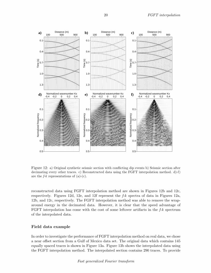
Figure 12a illustrates another synthetic seismic section which contains events with con-flicting dips with the total number of traces equal to 81. The decimated data and the



a)

0.1

0.4

0.7

1.0

1.3

Tim

e (s

)100 500 900

Distance (m) b)

0.1

0.4

0.7

1.0

1.3T

ime

(s)

100 500 900Distance (m) c)

0.1

0.4

0.7

1.0

1.3

Tim

e (s

)

100 500 900Distance (m)

d)

0.1

0.2

0.3

0.4

0.5

Nor

mal

ized

freq

uenc

y


0.1

0.2

0.3

0.4

0.5

Nor

mal

ized

freq

uenc

y


0.1

0.2

0.3

0.4

0.5

Nor

mal

ized

freq

uenc

y


Figure 12: a) Original synthetic seismic section with conflicting dip events b) Seismic section afterdecimating every other traces. c) Reconstructed data using the FGFT interpolation method. d)-f)are the f-k representations of (a)-(c).

reconstructed data using FGFT interpolation method are shown in Figures 12b and 12c,respectively. Figures 12d, 12e, and 12f represent the f-k spectra of data in Figures 12a,12b, and 12c, respectively. The FGFT interpolation method was able to remove the wrap-around energy in the decimated data. However, it is clear that the speed advantage ofFGFT interpolation has come with the cost of some leftover artifacts in the f-k spectrumof the interpolated data.

Field data example

In order to investigate the performance of FGFT interpolation method on real data, we chosea near offset section from a Gulf of Mexico data set. The original data which contains 145equally spaced traces is shown in Figure 13a. Figure 13b shows the interpolated data usingthe FGFT interpolation method. The interpolated section contains 290 traces. To provide



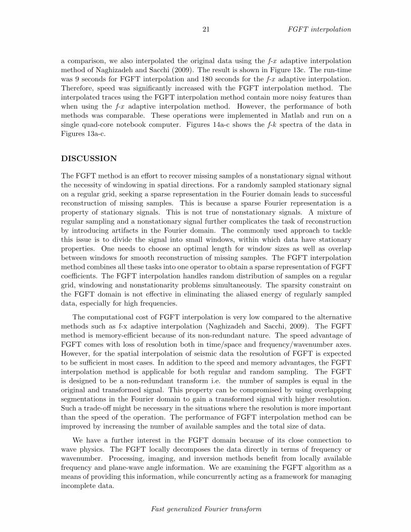
a comparison, we also interpolated the original data using the f-x adaptive interpolationmethod of Naghizadeh and Sacchi (2009). The result is shown in Figure 13c. The run-timewas 9 seconds for FGFT interpolation and 180 seconds for the f-x adaptive interpolation.Therefore, speed was significantly increased with the FGFT interpolation method. Theinterpolated traces using the FGFT interpolation method contain more noisy features thanwhen using the f-x adaptive interpolation method. However, the performance of bothmethods was comparable. These operations were implemented in Matlab and run on asingle quad-core notebook computer. Figures 14a-c shows the f-k spectra of the data inFigures 13a-c.

DISCUSSION

The FGFT method is an effort to recover missing samples of a nonstationary signal withoutthe necessity of windowing in spatial directions. For a randomly sampled stationary signalon a regular grid, seeking a sparse representation in the Fourier domain leads to successfulreconstruction of missing samples. This is because a sparse Fourier representation is aproperty of stationary signals. This is not true of nonstationary signals. A mixture ofregular sampling and a nonstationary signal further complicates the task of reconstructionby introducing artifacts in the Fourier domain. The commonly used approach to tacklethis issue is to divide the signal into small windows, within which data have stationaryproperties. One needs to choose an optimal length for window sizes as well as overlapbetween windows for smooth reconstruction of missing samples. The FGFT interpolationmethod combines all these tasks into one operator to obtain a sparse representation of FGFTcoefficients. The FGFT interpolation handles random distribution of samples on a regulargrid, windowing and nonstationarity problems simultaneously. The sparsity constraint onthe FGFT domain is not effective in eliminating the aliased energy of regularly sampleddata, especially for high frequencies.

The computational cost of FGFT interpolation is very low compared to the alternativemethods such as f-x adaptive interpolation (Naghizadeh and Sacchi, 2009). The FGFTmethod is memory-efficient because of its non-redundant nature. The speed advantage ofFGFT comes with loss of resolution both in time/space and frequency/wavenumber axes.However, for the spatial interpolation of seismic data the resolution of FGFT is expectedto be sufficient in most cases. In addition to the speed and memory advantages, the FGFTinterpolation method is applicable for both regular and random sampling. The FGFTis designed to be a non-redundant transform i.e. the number of samples is equal in theoriginal and transformed signal. This property can be compromised by using overlappingsegmentations in the Fourier domain to gain a transformed signal with higher resolution.Such a trade-off might be necessary in the situations where the resolution is more importantthan the speed of the operation. The performance of FGFT interpolation method can beimproved by increasing the number of available samples and the total size of data.

We have a further interest in the FGFT domain because of its close connection towave physics. The FGFT locally decomposes the data directly in terms of frequency orwavenumber. Processing, imaging, and inversion methods benefit from locally availablefrequency and plane-wave angle information. We are examining the FGFT algorithm as ameans of providing this information, while concurrently acting as a framework for managingincomplete data.



a)

0.1

0.7

1.3

Tim

e (s

)

500 2500 4500 6500Distance (m)

b)

0.1

0.7

1.3

Tim

e (s

)

500 2500 4500 6500Distance (m)

c)

0.1

0.7

1.3

Tim

e (s

)

500 2500 4500 6500Distance (m)

Figure 13: a) A near offset section form the Gulf of Mexico data set. b) Interpolated data usingthe FGFT interpolation method. c) Interpolated data using f-x adaptive interpolation method(Naghizadeh and Sacchi, 2009).



a)

0.1

0.2

0.3

0.4

0.5

Nor

mal

ized

freq

uenc

y-0.4 -0.2 0 0.2 0.4Normalized wavenumber Kx b)

0.1

0.2

0.3

0.4

0.5

Nor

mal

ized

freq

uenc

y

-0.4 -0.2 0 0.2 0.4Normalized wavenumber Kx c)

0.1

0.2

0.3

0.4

0.5

Nor

mal

ized

freq

uenc

y


Figure 14: a)-c) are the f-k representations of Figures 13a-13c.

CONCLUSIONS

The FGFT is a fast and efficient way of analyzing nonstationary signals and identifyingtheir time-frequency evolution. We used FGFT inside a least-squares fitting algorithm tointerpolate nonstationary seismic data. The method has the ability to cope with rapidand local changes of dip information in the seismic data. For randomly sampled dataon a regular grid, we seek a sparse representation in the FGFT domain to recover themissing samples. For regularly sampled data, the FGFT interpolation method utilizes thelow frequency portion of data for beyond-alias reconstruction of the high frequencies. Theproposed method is very fast and less demanding on computational memory compared to thealternative methods. The extension of FGFT interpolation to multidimensional applicationsis a straightforward task because in principle, it involves simple multidimensional Fouriertransforms.

ACKNOWLEDGEMENTS

We thank the financial support of the sponsors of the Consortium for Research in ElasticWave Exploration Seismology (CREWES) at the University of Calgary. We would also liketo thank Dr. Mauricio Sacchi for his inspiring discussions and useful comments.

REFERENCES

Abma, R. and N. Kabir, 2005, Comparison of interpolation algorithms: The Leading Edge,24, 984–989.

Beylkin, G., R. Coifman, and V. Rokhlin, 1991, Fast wavelet transforms and numericalalgorithms: Comm. on Pure and Appl. Math., 44, 141–183.



Brown, R. A., M. L. Lauzon, and R. Frayne, 2010, A general description of linear time-frequency transforms and formulation of a fast, invertible transform that samples thecontinuous s-transform spectrum nonredundantly: IEEE Trans. Signal Processing, 58,281–290.

Candes, E. J., L. Demanet, D. L. Donoho, and L. Ying, 2005, Fast discrete curvelet trans-forms: Multiscale Modeling and Simulation, 5, 861–899.

Candes, E. J. and D. L. Donoho, 2004, New tight frames of curvelets and optimal represen-tations of objects with piecewise-c2 singularities: Comm. on Pure and Appl. Math., 57,219–266.

Claerbout, J., 1992, Earth Soundings Analysis: Processing Versus Inversion: BlackwellScience.

Darche, G., 1990, Spatial interpolation using a fast parabolic transform: 60th AnnualInternational Meeting, SEG, Expanded Abstarcts, 1647–1650.

Duijndam, A. J. W., M. A. Schonewille, and C. O. H. Hindriks, 1999, Reconstruction ofband-limited signals, irregularly sampled along one spatial direction: Geophysics, 64,524–538.

Hennenfent, G. and F. J. Herrmann, 2008, Simply denoise: Wavefield reconstruction viajittered undersampling: Geophysics, 73, V19–V28.

Hestenes, M. R. and E. Stiefel, 1952, Methods of conjugate gradients for solving linearsystems: Journal of Research of the National Bureau of Standards, 49, 409–436.

Liu, B., 2004, Multi-dimensional reconstruction of seismic data: PhD thesis, University ofAlberta.

Margrave, G. F., D. Henley, M. P. Lamoureux, V. Iliescu, and J. Grossman, 2003, Gabordeconvolution revisited: SEG Expanded Abstracts, 22, 714–718.

Menke, W., 1989, Geophysical Data Analysis: Discrete Inverse Theory: Academic Press.Naghizadeh, M. and M. D. Sacchi, 2009, f-x adaptive seismic-trace interpolation: Geo-

physics, 74, V9–V16.——– 2010, On sampling functions and Fourier reconstruction methods: Geophysics, Ac-

cepted for publication.Sacchi, M. D., T. J. Ulrych, and C. J. Walker, 1998, Interpolation and extrapolation using

a high-resolution discrete fourier transform: IEEE Transaction on Signal Processing, 46,31–38.

Scales, J. A. and A. Gersztenkorn, 1988, Robust methods in inverse theory: Inverse Prob-lems, 4, 1071–1091.

Spitz, S., 1991, Seismic trace interpolation in the F-X domain: Geophysics, 56, 785–794.Stockwell, R. G., L. Mansinha, and R. P. Lowe, 1996, Localization of the complex spectrum:

The S transform: IEEE Trans. Signal Processing, 44, 998–1001.Tikhonov, A. N. and A. V. Goncharsky, 1987, Ill-posed problems in the natural sciences:

MIR Publisher.Trad, D., T. J. Ulrych, and M. D. Sacchi, 2002, Accurate interpolation with high-resolution

time-variant radon transforms: Geophysics, 67, 644–656.Zwartjes, P. and A. Gisolf, 2006, Fourier reconstruction of marine-streamer data in four

spatial coordinates: Geophysics, 71, V171–V186.


Date post:	14-Apr-2018
Category:	Documents
Upload:	phungque
View:	216 times
Download:	2 times

Seismic data interpolation using a fast generalized ...mostafan/Files/Papers/fgft_GEO2011.pdf ·...

Documents