University of Montana University of Montana ScholarWorks at University of Montana ScholarWorks at University of Montana Graduate Student Theses, Dissertations, & Professional Papers Graduate School 2007 Seismic Reflection and Gravity Constraints on the Bedrock Seismic Reflection and Gravity Constraints on the Bedrock Configuration in the Greater East Missoula Area Configuration in the Greater East Missoula Area Frank Janiszewski The University of Montana Follow this and additional works at: https://scholarworks.umt.edu/etd Let us know how access to this document benefits you. Recommended Citation Recommended Citation Janiszewski, Frank, "Seismic Reflection and Gravity Constraints on the Bedrock Configuration in the Greater East Missoula Area" (2007). Graduate Student Theses, Dissertations, & Professional Papers. 1219. https://scholarworks.umt.edu/etd/1219 This Thesis is brought to you for free and open access by the Graduate School at ScholarWorks at University of Montana. It has been accepted for inclusion in Graduate Student Theses, Dissertations, & Professional Papers by an authorized administrator of ScholarWorks at University of Montana. For more information, please contact [email protected].
Transcript
University of Montana University of Montana
ScholarWorks at University of Montana ScholarWorks at University of Montana
Graduate Student Theses, Dissertations, & Professional Papers Graduate School
2007
Seismic Reflection and Gravity Constraints on the Bedrock Seismic Reflection and Gravity Constraints on the Bedrock
Configuration in the Greater East Missoula Area Configuration in the Greater East Missoula Area
Frank Janiszewski The University of Montana
Follow this and additional works at: https://scholarworks.umt.edu/etd
Let us know how access to this document benefits you.
Recommended Citation Recommended Citation Janiszewski, Frank, "Seismic Reflection and Gravity Constraints on the Bedrock Configuration in the Greater East Missoula Area" (2007). Graduate Student Theses, Dissertations, & Professional Papers. 1219. https://scholarworks.umt.edu/etd/1219
This Thesis is brought to you for free and open access by the Graduate School at ScholarWorks at University of Montana. It has been accepted for inclusion in Graduate Student Theses, Dissertations, & Professional Papers by an authorized administrator of ScholarWorks at University of Montana. For more information, please contact [email protected].
SEISMIC REFLECTION AND GRAVITY CONSTRAINTS ON THE BEDROCK
CONFIGURATION IN THE GREATER EAST MISSOULA AREA
By
Frank David Janiszewski
B.S., Michigan Technological University
Houghton, Michigan, 2004
Thesis
presented in partial fulfillment of the requirements for the degree of
Master of Science
in Geophysics
The University of Montana Missoula, MT
Spring 2007
Approved by:
Dr. David A. Strobel, Dean Graduate School
Dr. Steven Sheriff
Geosciences
Dr. James Sears Geosciences
Dr. Jesse Johnson
Computer Sciences
Janiszewski, Frank, M.S., May 2007 Geophysics Seismic Reflection and Gravity Constraints on the Bedrock Configuration in the Greater East Missoula Area Chairperson: Steven Sheriff
The greater East Missoula, MT area is the site of numerous studies to track possible groundwater contamination from the EPA Superfund Site at the Milltown Dam. The accuracy of these groundwater models depends on many factors, one of which is the accuracy to which the bedrock topography is mapped. Currently, a map based heavily on a gravity survey provides the most detailed map of the bedrock. The accuracy of this map may be improved through the use of seismic reflection techniques, better estimates of the density contrast used in the gravity modeling, and by extending the gravity survey to include more data and a broader area.
The seismic reflection technique used to supplement the gravity data is the optimum offset technique. This method simplifies field collection of the data and processing of the data. The final result of this method is a seismic section showing the depth to different reflectors in the subsurface, one of which is the bedrock. In order to improve the estimate of the density contrast used in the gravity modeling, the homogeneity of the valley fill was tested. This was done by comparing the results from two different modeling programs, one of which let the density contrast vary, to see if there was an improvement in the final result. The gravity survey was also extended to incorporate a larger area and more data.
The results show that seismic reflection can be used to improve the depth estimate in the valley where the depth is shallow and that the density contrast is most likely homogeneous. The extended gravity survey provided more data to work with and the final result is a map of the bedrock topography for the greater East Missoula Area that incorporates all currently known data and provides a sufficiently accurate estimate of the depth to be used in groundwater models.
ii
To my Parents for all they have given me
iii
TABLE OF CONTENTS Page ABSTRACT...............................................................................................................ii
LIST OF FIGURES ...................................................................................................v
LIST OF TABLES.....................................................................................................vii
LIST OF APPENDICES............................................................................................viii
2 Summary of seismic results from Bonner School Field ..............................31
3 Summary of seismic results from Deer Creek Road....................................31
4 Summary of seismic results from Hellgate Park..........................................31
5 Summary of results using GI3 with no initial model...................................58
6 Summary of results using GI3 with an initial model ...................................58
7 Summary of results using GRAVMOD3D with A = 0.001.........................60
8 Summary of results using GRAVMOD3D with A = 0.01...........................60
9 Summary of results using GRAVMOD3D with A = 0.1.............................61
10 Summary of results using GRAVMOD3D with A = 1.0.............................61
11 Summary of results using GI3 with the complete data set............................80
vii
LIST OF APPENDICIES
Appendix Page A Known depth to bedrock locations and values ..................................98
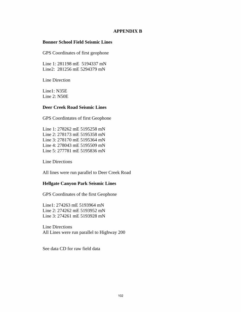
B Seismic Line Location Details ..........................................................102
C Detailed Seismic Methods ................................................................103
D Detailed Gravity Methods.................................................................104
E Equipment Specifications .................................................................106
viii
INTRODUCTION
In west-central Montana, Milltown Valley (Figure 1), located at the confluence of
the Clark Fork River and the Blackfoot River, has been the subject of intense scrutiny
since the discovery of heavy metal groundwater contamination in 1981. The area is
currently an Environmental Protection Agency Superfund site. The cleanup effort will
involve removal of Milltown dam and some of the contaminated sediments behind it
(Milltown Reservoir Sediments EPA Superfund Site). A chief concern of the citizens in
the area is how the contamination will move downstream after the removal of the dam.
The aquifer below Milltown Valley is directly connected to the Missoula Valley Aquifer,
which serves as the main drinking water supply for the city of Missoula, Montana.
Several studies have been completed to address the question of where the contamination
may go [Associates, 1987; Camp, 1989; Woessner, 1993; Woessner, 1984; Woessner,
1982].
A key component of these studies was the determination of the configuration of
bedrock surface beneath the valley. The three-dimensional configuration of bedrock
surface plays an important role in local groundwater flow. A bedrock map (Gestring,
1994) was used as an input for the groundwater models (Figure 2). Gestring’s (1994)
map of the bedrock was based on bedrock exposures, drill core data and some limited
seismic data. The limited amount of bedrock exposures in the valley and sporadic
spacing of the wells left large areas in the study with little or no data. The lack of data
and control points led to the mapping of some suspect features. The accuracy of this map
was not great enough to support the grid size of 91.4 meters used in the groundwater
1
Fi
gure
1: T
opog
raph
ic m
ap o
f the
stud
y ar
ea.
The
area
out
lined
in b
lue
is th
e or
igin
al st
udy
area
. Th
e ar
ea o
utlin
ed in
red
is th
e ex
tend
ed st
udy
area
. C
oord
inat
e sy
stem
is M
onta
na S
tate
Pla
ne N
AD
83.
2
Figu
re 2
. B
edro
ck m
odel
of G
estri
ng (1
994)
, bas
ed o
n be
droc
k ou
tcro
ps, w
ell i
nfor
mat
ion
and
seis
mic
line
s. T
his p
art o
f the
val
ley
outli
ned
in b
lue
on F
igur
e 1.
3
model constructed by Gestring. The resulting groundwater model proved difficult to
calibrate [Nyquest, 2001].
To improve on this map, Nyquest (2001) supplemented Gestring’s map with a
gravity survey of the area. By collecting data at 394 gravity stations and combining those
data points with gravity data from the National Geophysical Data Center and the U.S.
Defense Mapping Agency, Nyquest (2001) created a regional gravity profile of the study
area. The gravity data were then used to create a depth-to-bedrock model and an
improved map of the bedrock surface (Figure 3). Nyquest’s (2001) map contained
considerably more detail than Gestring’s and differed in many places. In addition to the
gravity measurements collected by Nyquest (2001), Anthony Bertholote collected 204
new gravity stations in 2006. The new gravity stations extend the survey area to the east
along the Clark Fork River and to the northeast along the Blackfoot River. In this thesis,
I use these new gravity measurements and my own seismic experiments to further
improve and extend the bedrock model.
My objective is to test previous results and possibly improve the bedrock surface
map in the Milltown Valley area through collection and analysis of seismic data, along
with reinterpretation of previously collected gravity data. Nyquest’s (2001) bedrock
surface map improved upon Gestring’s (1994) map. However, Nyquest’s (2001)
interpretation of the gravity data did not take into account the possible heterogeneity of
the valley fill. Nyquest (2001) used a density contrast of -725 kg/m3 for the valley fill in
his model. The density contrast was found by modeling the gravity data with a range of
density contrasts. The density contrast that minimized the error between known depths
(from wells and drill cores) and the modeled depth was assumed to be correct for the
4
Figu
re 3
: N
yque
st’s
(200
1) d
epth
to b
edro
ck m
odel
. Th
is m
odel
was
cre
ated
by
inve
rting
app
roxi
mat
ely
400
grav
ity m
easu
rem
ents
co
llect
ed th
roug
hout
the
valle
y. T
his m
ap sh
ows m
any
feat
ures
that
wer
e no
t pre
viou
sly
map
ped
in G
estri
ngs (
1994
) dep
th to
bed
rock
m
odel
. Th
is m
ap is
in th
e sa
me
loca
tion
as th
e m
ap p
rese
nted
in fi
gure
2.
5
entire valley. In order to test if the density contrast varies with depth, the reinterpretation
of the gravity data I performed involved allowing the density of the valley fill to increase
with depth. The seismic reflection data collected throughout the area provide an
additional control on the interpreted gravity data. By comparing the interpreted seismic
data to the gravity model the accuracy of the gravity model can be validated. Also, there
are many known depth-to-bedrock data throughout the valley from previous seismic data,
drill core data and groundwater wells completed to bedrock (Appendix A) which can be
used to validate the final bedrock map. The final product is a map of bedrock elevations
that is constrained with all available data, which includes: depth to bedrock from drill
core data from cores and wells completed to bedrock, bedrock outcrops, gravity data, and
seismic refraction and reflection data.
6
SEISMIC DATA COLLECTION AND INTERPRETATION
Introduction
Nyquest (2001) presents a depth to bedrock model based mainly on gravity
measurements. Parts of this map are not well constrained due to lack of depth control
(i.e. drill core and well data) and sparse gravity measurements. Some of these areas
appear to be sufficiently shallow to conduct an engineering-scale seismic reflection
survey to test Nyquest’s (2001) interpretations. I conducted three surveys at locations
throughout the valley based on access and proximity to wells. Nyquest (2001) referenced
the seismic refraction data used by Gestring (1994) to construct his bedrock model. The
data from these seismic surveys is contained in Appendix A, which consists of all known
depth to bedrock points.
Seismic reflection techniques were chosen over seismic refraction techniques for
two main reasons. First, seismic refraction surveys had already been successfully
completed in the survey area. I wanted to test seismic reflection methods to see if I could
produce similar results. Second, the increase computing technology since the 1970’s and
1980’s has drastically reduced the time it takes to manipulate and process seismic
reflection data. With the computing power available the processing of seismic reflection
data takes much less time than it did 30 years ago and results can be found relatively
quickly.
I collected seismic data along ten lines located throughout the study area as seen
in Figure 4. The lines collected near Bonner Elementary school tested the utility of
seismic reflection techniques for determining depth to bedrock. The lines collected in the
Bandmann flats were used to directly compare results from the gravity interpretation and
7
Fi
gure
4:
Loca
tion
of th
e se
ism
ic li
nes c
olle
cted
in 2
005.
Thr
ee se
ism
ic li
nes w
ere
colle
cted
in th
e H
ellg
ate
Can
yon
in H
ellg
ate
Park
. Fi
ve se
ism
ic li
nes w
ere
colle
cted
in th
e ce
ntra
l par
t of t
he st
udy
area
alo
ng D
eer C
reek
Roa
d. T
wo
seis
mic
line
s wer
e co
llect
ed a
t the
ea
st e
nd o
f the
stud
y ar
ea b
ehin
d B
onne
r Ele
men
tary
Sch
ool.
8
the seismic interpretation. The lines collected in Hellgate Park were a test of the
maximum depth possible using engineering scale seismic reflection techniques with the
available equipment; the seismic source used is the main limitation.
Seismic reflection surveys measure the time taken for an elastic wave to travel
from a source through the subsurface to an interface between rock types where it is
reflected and returns to the surface, where it is recorded by a receiver. The receiver
measures the ground deformation caused by the returning elastic wave and the travel time
of the wave from the source to the receiver. An array of receivers is used to collect these
data over the length of the survey line. For this survey I used a Bison Instruments
accelerated weight drop as the energy source (Figure 5). To record the arrivals of the
refraction and reflection waves I used a Geometrics Smartseis 24 Channel seismograph
and twenty-four 40 hertz geophones.
I collected the seismic data with the optimum offset-technique [Pullan and
Hunter, 1991; Steeples and Miller, 1991], the offset being the distance between the
source and a geophone. For each source location there are at least three types of waves
that return to the receivers on the surface: the refracted wave or direct wave, the reflected
wave and ground roll, all arriving at different times. The optimum offset distance is the
offset from the source to a geophone at which the reflected wave arrives between the
direct wave and the ground roll (Figure 6). The optimum offset technique constructs a
seismic section one seismic trace at a time, one from each location of the Bison
Instrument signal source.
The optimum offset technique streamlines the field collection process, allowing
the geophone array to remain stationary and only requiring the shot point to move. The
9
Figure 5: Bison Industries elastic wave generator. This accelerated weight drop system works by dropping a steel beam (yellow arrow) into the ground. The beam is lifted using a hydraulic ram (blue arrow) and is accelerated into the ground using a large elastic band (red arrow). This source is capable of generating a large amount of seismic energy.
10
Fi
gure
6:
The
optim
um o
ffse
t tec
hniq
ue fo
r sei
smic
refle
ctio
n su
rvey
s. T
he p
anel
on
the
left
show
s the
bas
ic p
rinci
ple
of th
e op
timum
off
set t
echn
ique
. A
sing
le g
eoph
one
is u
sed
to re
cord
the
arriv
al o
f the
diff
eren
t wav
es.
The
geop
hone
and
the
sour
ce a
re
sepa
rate
d by
the
optim
um o
ffse
t. E
ach
geop
hone
(lab
eled
G) a
nd so
urce
(lab
eled
S) p
air r
epre
sent
one
trac
e of
the
final
seis
mic
se
ctio
n. T
he p
anel
on
the
right
show
s why
opt
imum
off
set w
orks
. Th
e re
flect
ed w
ave
from
bed
rock
arr
ives
afte
r the
firs
t arr
ival
but
be
fore
the
grou
nd ro
ll an
d ai
rwav
e. T
his s
impl
ifies
the
colle
ctio
n an
d pr
oces
sing
of t
he se
ism
ic d
ata.
Fig
ure
take
n fr
om P
ulla
n an
d H
unte
r (19
91).
11
optimum offset is specific to each location and set of subsurface conditions and can be
determined after the data have been collected. The primary benefit of the optimum offset
technique over other seismic reflection techniques (common midpoint gathers and
common shot point gathers) is that it simplifies the processing. In both common
midpoint gathers and common shot point gathers the processing required to generate a
final section requires more steps and more user inputs. A common midpoint survey
processed by two different processors may produce different results, based on each
processor’s choice of inputs [Reynolds, 1997]. An optimum offset survey requires fewer
steps and less user inputs to process, reducing the likelihood of a processing mistake and
increasing the repeatability of the experiment.
Seismic Data Collection
For each seismic reflection line, the geophones were arranged in a straight line
with a spacing of two meters. The Bison elastic wave generator was initially positioned
12 to 30 meters in line from the first geophone depending on estimates of the depth to
bedrock from Nyquest’s (2001) map or water wells located nearby. The source was
triggered three times, and the data from each triggering were added together in phase to
cancel random events and thereby improve the signal to noise ratio. The source was then
moved closer to the first geophone by two meters, and the process repeated. This entire
procedure was repeated between 17 and 30 times depending on site constraints. The
location of the first geophone was recorded using a handheld GPS unit and the direction
of the line was recorded using a Brunton Compass (Appendix B).
12
Seismic Data Interpretation
Following acquisition in the field, I used Seismic Unix NT to do the initial
processing of the seismic data. Seismic Unix NT was also used to calculate the offset
and midpoint of each shot from each of the 24 geophones. The offset is the distance
between any geophone and the source, and the midpoint is the location halfway between
each geophone and the source. All remaining processing steps were completed using
Seismic Unix, a freely distributed Unix-based processing package available from the
Colorado School of Mines.
During processing, one starts with raw data (Figure 7), determines and collates the
traces at optimal offset for each source location, and proceeds until an interpretable
seismic section is created. The ultimate goal is to come up with a result from which one
can determine the depth to the velocity contrast between the valley fill and underlying
bedrock. For each survey location the data from the first shot at each location was
analyzed to determine what the optimum offset should be. By analyzing the seismic
signal traces in the section, I determined which trace had the reflected data arriving
between the direct wave and the ground roll (Figure 8). Table 1 shows the optimum
offset value used for each seismic line. After the optimum offset was determined, the
traces that had an offset equal to the optimum offset were extracted from the raw data and
placed into a new file. For each source location in a survey there was only one trace that
corresponded to the optimum offset, meaning if the survey contained 15 source locations
then the new file would contain 15 traces. The result being a seismic profile of 15 traces,
each separated by 2 meters, all collected at the optimum offset.
13
Location Line Optimum Offset
Value (m) Bonner School 1 12 Bonner School 2 12 Deer Creek Rd. 1 28 Deer Creek Rd. 2 36 Deer Creek Rd. 3 36 Deer Creek Rd. 4 32 Deer Creek Rd. 5 36 Hellgate Park 1 30 Hellgate Park 2 30 Hellgate Park 3 30
Location Layer Velocity (m/s)
1 600 2 1300 Bonner School 3 2800 1 600 2 1100 Deer Creek Rd 3 2500 1 600 2 1500 Hellgate Park 3 **
Table 1. Velocity of the three layers for each location along with the optimum offset used at each location. The third layer velocity for Hellgate Park is not listed because the seismic energy did not penetrate to the third layer.
14
Figure 7: An example of the raw seismic field data collected. The raw field data contains all of the traces from each source location. The next step in processing is extracting the traces that correspond to the optimum offset distance.
15
Figure 8: Time distance plot showing the three types of waves present and how the optimum offset is chosen. The waves highlighted by the green box are the arrivals of the direct waves. The waves highlighted by the red box are ground roll and air shock waves arriving. In between the two are the reflected waves of interest, highlighted by yellow. The optimum offset is chosen so that the reflected waves arrive after the direct wave but before the ground roll. The offset chosen for this section is 28 meters.
16
After collating the optimum offset traces, the traces were filtered to remove
unwanted noise and enhance the signal and then were gained using an automatic gain
control. Filtering of seismic data involves removing certain frequencies that contain
noise (i.e. highway vibrations, wind, power line interference, etc). This is typically done
using a bandpass filter which truncates low and high frequencies, leaving only the
seismic waves generated by the source. I employed 40 Hz geophones, and the signal
source has most of its power between the frequencies of 5 and 70 Hz [Thompson, 1997],
so filtering out frequencies above and below this range should leave coherent reflection
data. Seismic Unix allows one to adjust the upper and lower cutoff frequencies until a
satisfactory seismic section results. The bandpass filter tapered from 30 Hz up to 45 Hz
and down from 120 Hz to 175 Hz. Looking at a representative section of raw data after
collation but before filtering (Figure 9) shows how noise can obscure reflectors. There is
low frequency noise present in the section that overpowers what could be reflectors.
Looking at the same data after the bandpass filter was applied (Figure 10) shows the
unwanted frequencies removed. What are left in the section are now coherent reflectors
without unwanted noise to obscure them (Figure 11). Looking at the frequency spectrum
of the data before and after the filtering (Figure 12), it is apparent that the low frequency
noise was removed, leaving the data between 30 and 120 Hz.
Gaining the data amplifies the seismic signals with increasing time, which
simplifies interpretation by making the reflectors more pronounced (Figure 13). Seismic
Unix uses automatic gain control which uses the average signal amplitude over a window
of time to adjust the gain over the whole seismic trace. The time window size can be
adjusted to increase or decrease the level of gain. The automatic gain control window
17
Figure 9: Deer Creek Road Line 2 raw data. Notice the low frequency noise present in the bottom half of the section.
18
Figure 10: The same data as seen in the previous figure from Deer Creek Road after the bandpass filter was applied. Notice that the low frequency noise that was present in the section has been removed. This leaves the features in the center of the section as the most prominent feature.
19
Figure 11: An example of the seismic data after trace extraction. The data went from containing over 600 traces to just 24 traces. The raw field data contained traces with offsets ranging from 2 meters to 60 meters. The extracted traces all have the same offset which corresponds to the optimum offset. The data was also filtered using a band pass filter to remove both high and low frequency noise.
20
Frequency Spectrum Pre Filter
Frequency Spectrum Post Filter
Figure 12: Frequency spectrum of the data shown in the previous two figures. The top panel shows the frequency spectrum of the unfiltered data and the bottom panel shows the frequency spectrum of the filtered data. In the unfiltered data there is a large amount of amplitude present in the low frequencies (below 35 Hz). Filtering the data removes the low frequencies while leaving frequencies that contain reflection data (40 to 130 Hz).
21
Figure 13: An example of seismic data that has been filtered and gained. The data is amplified using automatic gain control. This increases and normalizes the signal making it easier to see and interpret what is happening. At this point the seismic data is ready for interpretation.
22
was set to 0.09 seconds. All data collected were processed in a similar manner using the
same filtering and gain parameters.
To interpret each line the velocity of the first layer needed to be determined. The
velocities of the layers are related to the first arrival times in the seismic record (Figure
14). The first arrivals are the direct wave traveling through the uppermost layer or
critically refracted waves from subsequently deeper layers [Reynolds, 1997]. To find the
velocity, the first arrival times are plotted on the y-axis and the distance between the
receivers are plotted on the x-axis (Figure 15). The points should all fall on a straight line
(time = distance / speed) and the inverse slope of the line yields the velocity of the layer.
Breaks in the slope of the line represent the next deepest layer, with the number of breaks
in slope representing the number of layers visible in the seismic section. An assumption
made in interpreting the data is that the velocity of each layer is consistent for the entire
depth extent of the layer, and the only changes in velocity occur at the interface of two
layers. For this assumption to hold the first arrival times for each layer have to lie along
a straight line. If the velocity changed gradually with depth then the plot of the first
arrivals would lie along a curve. Looking at a representative time-distance plot (Figure
15), the first arrivals plot along straight lines with an R2 value of 0.98 or higher, meaning
the assumption of a constant velocity within each layer holds true.
Table 1 shows the velocity of the different layers for each location, and Figure 16
represents the data graphically. The velocity of the first layer is consistent at each
location, approximately 600 m/s. This falls within the ranges of dry sand (200 to 1000
m/s) and near surface (less than 2 km) sand and gravel (400 to 2300 m/s) [Reynolds,
1997]. The velocity of the second layer varies slightly from location to location, ranging
23
Figu
re 1
4: F
irst a
rriv
al p
icks
from
a ti
me
dist
ance
plo
t. T
he fi
rst a
rriv
als a
re th
e di
rect
wav
e ar
rivin
g at
the
geop
hone
and
can
be
seen
as
a d
efle
ctio
n of
the
trace
to th
e le
ft. P
lotti
ng a
stra
ight
line
thro
ugh
the
first
arr
ival
s det
erm
ines
the
velo
city
of e
ach
laye
r. In
this
pl
ot th
ere
are
thre
e di
stin
ct c
hang
es in
the
slop
e of
the
first
arr
ival
s, co
rres
pond
ing
to th
ree
diff
eren
t lay
ers.
24
Tim
e D
ista
nce
Plot
y =
1.66
27x
+ 6.
4036
R2 =
0.9
949
y =
0.99
82x
+ 25
.804
R2 =
0.9
852
y =
0.35
x +
52.9
71R
2 = 0
.986
01020304050607080
010
2030
4050
60
Dist
ance
(m)
Time (msec)
Laye
r1La
yer2
Laye
r3Li
near
(Lay
er1)
Line
ar (L
ayer
2)Li
near
(Lay
er3)
Figu
re 1
5: L
inea
r vel
ocity
ana
lysi
s plo
t. T
he x
axi
s sho
ws t
he d
ista
nce
of th
e ge
opho
ne fr
om th
e so
urce
loca
tion
and
the
y-ax
is sh
ows
the
arriv
al ti
me
in m
illis
econ
ds o
f the
firs
t arr
ival
of s
eism
ic e
nerg
y. T
here
are
thre
e gr
oups
of p
oint
s, ea
ch g
roup
falli
ng a
long
a
stra
ight
line
with
a sp
ecifi
c sl
ope.
The
slop
e of
the
line
is th
e in
vers
e of
the
velo
city
of e
ach
laye
r. T
he R
2 val
ue fo
r eac
h lin
e is
clo
se
to 1
, mea
ning
stat
istic
ally
the
poin
ts fa
ll al
ong
a st
raig
ht li
ne.
The
colo
rs o
f the
line
s cor
resp
ond
to th
e lin
es th
roug
h th
e fir
st a
rriv
als
on th
e pr
evio
us fi
gure
.
25
0
~2800~2500
~1300
~1100
~1500
~600
~600
~600
Hellgate Park Deer Creek road Bonner School
Location
Velo
city
(m/s
)
Layer 1
Layer 2
Layer 3
Figure 16: Results from the velocity analysis of the seismic data at three different locations across the valley. The velocity of each layer is the result of averaging the velocity data from a number of source locations on each line collected. The velocity of each layer is consistent across the valley. Hellgate park does not have a layer 3 velocity because the third layer is to deep to see. Velocities are listed as m/s.
26
from 1100 m/s along Deer Creek Road to 1900 m/s in Hellgate Park. The velocity
increase between layer 1 and layer 2 is due to the valley-fill being saturated with water
[Reynolds, 1997]. The seismic lines collected behind Bonner Elementary school and
along Deer Creek Road show a third layer in the direct wave arrivals. This layer has a
velocity of approximately 2800 m/s which matches the velocity of the underlying
bedrock (2500 to 3000 m/s) [Blackhawk Geosciences, 1990]. The velocities listed were
found by averaging the velocity of each layer found using each source location.
Appendix C contains details on the processing steps used.
The final step in interpreting the seismic data consists of picking the reflectors on
each of the processed seismic sections. In some of the sections the reflectors are fairly
apparent, while, for others, choosing reflectors requires more finesse. Once the reflectors
are chosen, the two-way travel time for each reflector can be determined. Multiplying
one half of the two-way travel time by the velocity of the first layer yields the depth of
the reflector. These reflectors can then be translated into depth to bedrock [Bradford,
2002; Goforth and Hayward, 1992; Steeples and Miller, 1998].
Seismic Results and Discussion
Two seismic lines were collected in the field north of Bonner Elementary
School at the east end of the study area (Figure 4). The first line consisted of 768 traces
collected from 24 geophones and 32 positions of the Bison signal source, resulting in 32
optimum offset traces. The second line contained 864 traces that resulted in 36 optimum
offset traces. Figures 17 and 18 show the final processed seismic sections from Bonner
Elementary. In both sections there are two prominent reflectors located above 0.1
27
Figure 17: Final interpreted seismic section from Bonner Elementary School Line 1. There are two possible reflectors interpreted on this section; one at approximately 13 meters and one at approximately 38meters. The trace separation is 2 meters.
28
Figure 18: Final interpreted section from Bonner Elementary School Line 2. There are two reflectors interpreted on this section; one at approximately 13 meters and a second at approximately 38 meters. The trace separation is 2 meters.
29
seconds, one at approximately 0.04 seconds and one at approximately 0.08 seconds.
Using the first arrivals to determine the velocity yields a velocity for the first layer of
approximately 600 m/s and a velocity of the second layer of approximately 1300 m/s.
Using this velocity and the two way travel times the depth of the first reflector is
approximately 13 meters deep, and the second reflector is 38 meters deep. The depths
of the first reflectors, at approximately 13 meters, are much shallower than the known
depth to bedrock of 38 meters from a well drilled approximately 50 meters to the north
east. I interpret this reflector to be the water table in the area. The velocity above and
below the reflector is approximately 600 m/s and 1300 m/s respectively, which is typical
for a change from dry sand to saturated sand. The second reflector in both sections
occurs at approximately 38 meters in depth, which matches the bedrock depth from the
well. This reflector is the strongest reflector in both sections and occurs at the same
depth in both sections. The velocity below the reflector is 2800 m/s , which is a typical
velocity for Belt Supergroup rocks [Blackhawk Geosciences, 1990]. Table 2 summarizes
the data from Bonner School Field.
Five seismic lines comprise the Deer Creek data set. These lines cross Bandmann
Flats in the central part of the study area (Figure 4), each containing contains 336 traces,
and resulted in 14 optimum offset traces per line. Figures 19 through 23 show the final
processed sections. These sections were collected along the road where there was less
control over environmental factors like road traffic and urban noise. Despite using
various gain functions and a multitude of different frequency filters, I was not able to
produce sections with signal-to-noise ratio as high as in the Bonner area. Consequently
the sections are more difficult to interpret than the sections from Bonner School Field.
Table 3. Summary of the results from the seismic lines collected along Deer Creek Road. Bedrock reflectors are highlighted in yellow.
Hellgate Canyon Park Line Reflector 2-way Travel Time (ms) Depth (m)
1 1 0.055 600 17 2 1 0.06 600 18 3 1 0.075 600 22
Table 4. Summary of the results from the seismic lines collected in Hellgate Canyon Park.
31
Figure 19: Final interpreted section from Deer Creek Road line 1. This section shows the arrival of the direct wave (green line) and two reflectors (yellow lines). The reflectors occur at 27 meters and 52 meters. The trace separation is 2 meters.
32
Figure 20: Final interpreted section from Deer Creek Road Line 2. This section shows two possible reflectors, one at 31 meters and one at 45 meters. The trace separation is 2 meters.
33
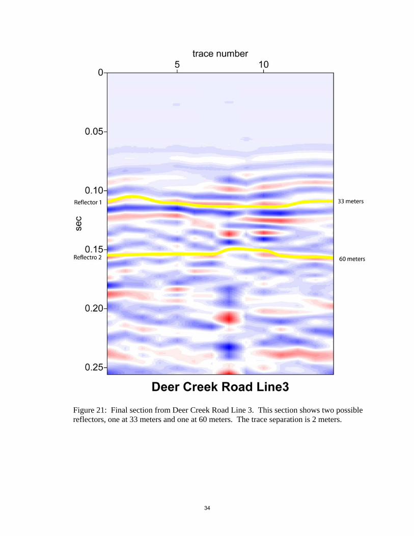
Figure 21: Final section from Deer Creek Road Line 3. This section shows two possible reflectors, one at 33 meters and one at 60 meters. The trace separation is 2 meters.
34
Figure 22: Final section from Deer Creek Road Line 4. This section shows the arrival of the direct wave and two possible reflectors. The first reflector is at 30 meters and the second reflector is at 52 meters. The trace separation is 2 meters.
35
Figure 23: Final interpreted section from Deer Creek Road Line 5. This section shows 2 possible reflectors, one at 30 meters and one at 52 meters. The trace separation is 2 meters.
36
DCR Line 1 (Figure 19) shows 2 prominent reflectors. The first reflector is located at
0.09 seconds and the second reflector is located at 0.135 seconds. Also visible in this
reflector is the direct wave, which can be seen at 0.055 seconds. DCR Line 2 (Figure
20) shows much less detail than Deer Creek Road line 1 but it is still possible to pick out
2 reflectors. The first reflector occurs at 0.105 seconds and the second at 0.13 seconds.
DCR line 3 (Figure 21) also shows 2 possible reflectors. The first reflector occurs at 0.11
seconds and the second reflector at 0.16 seconds. DCR line 4 (Figure 22) also lacks in
detail, but there are two reflectors at 0.099 seconds and 0.14 seconds. The direct wave is
also visible in this section at 0.075 second. The final seismic line collected along Deer
Creek Road, line 5 (Figure 23), shows two reflectors, one at 0.10 seconds and one at 0.14
seconds. Using the first arrivals of the refracted waves from a number of different source
locations along Deer Creek Road yields an average first layer velocity of approximately
600 m/s and an average second layer velocity of 1100 m/s, which are used to calculate
the depth of the reflectors in each section.
Line 1 (Figure 19) along the road showed the clearest reflections and was the
easiest to interpret. Line 1 showed two reflections and the arrival of the direct wave. The
reflector that occurs at 0.055 seconds is the direct wave arriving. By dividing the offset
for this line (28 meters) by the velocity of the first layer (600 m/s) the approximate time
of the arrival of the direct wave can be calculated (0.05 seconds), which matches the time
of the first reflector. The second reflector occurs at a depth of 27 meters which is close to
the depth of the water table (25 meters) reported at a nearby irrigation well (Canyon
River Irrigation Well). The velocity change at this reflector matches the velocity change
seen going from dry sand to wet sand. The final reflector in this section occurs at 52
37
meters in depth. This is the bedrock reflection, which is confirmed by the velocity
change (1100 m/s above, 2500 m/s below).
Deer Creek Road line 2 (Figure 20) is difficult to interpret. The data were
collected near a highway overpass, which introduced noise of a similar frequency to the
reflections (between 45 and 120 Hz). The two reflectors seen in this section occur at 32
meters and 45 meters. The velocity change at each reflector confirms that the reflections
are the water table and the bedrock respectively.
The third line (Figure 21) collected along Deer Creek Road was also collected
near the highway overpass so much of its data was also masked by noise from the
highway. The two reflectors visible in this section occur at 33 meters and 60 meters.
The velocity change at each reflector again indicates that they are the water table and
bedrock.
Line 4 (Figure 22) from Deer Creek Road was collected in an area of damp soil.
Because of this, the signal was highly attenuated and the seismic section shows only
weak reflections. There are two possible reflections in this section, the first occurs at 29
meters and the second occurs at 52 meters. The velocity change at each reflector
suggests that they are the water table and bedrock respectively.
The final section (Figure 23) along Deer Creek Road was collected in similar
conditions to line 4 but shows a slightly better signal to noise ratio. There are two
reflectors visible in this section, the first at 30 meters and the second at 52 meters. Again
these are water table and bedrock.
Three seismic lines were collected in Hellgate Canyon Park at the west end of the
study area, each containing 360 traces, and resulted in 15 optimum offset traces. Hellgate
38
Canyon Park Line 1 (Figure 24) shows one prominent reflector that occurs at 0.055
seconds. Hellgate Canyon Park Line 2 (Figure 25) also shows one prominent reflector
that occurs at 0.06 seconds. The final seismic line (Figure 26) collected in Hellgate
Canyon Park also shows one prominent reflector occurring at 0.075 seconds. Below the
first reflector in each section are what appear to be additional reflectors having the same
general shape as the first reflector in each section. These are multiples of the first
reflectors. Multiples occur when seismic energy is “bouncing” around through the
subsurface. Multiples of dipping beds generally have a steeper gradient than the original
reflector that produces them. In the sections from Hellgate Canyon Park it appears that
the reflections seem to increase in steepness as they get deeper.
Using the first arrival times of the refracted waves yields a velocity of the first
layer approximately 600 m/s. In this area the bedrock was too deep to return seismic
reflection or refraction data. The only reflection visible in the sections occurs at
approximately 18 – 20 meters. The velocity changes from 600 m/s above the reflector to
1500 m/s below the reflector, meaning that the reflection is most likely the water table.
Below the water table reflection the sections contain multiples of the water table and
noise. Table 4 summarizes the data from Hellgate Canyon Park
Conclusion
The seismic results from Bonner school and Deer Creek road confirm the results
from Nyquest (2001), matching closely both his results modeled from gravity and known
depth to bedrock from wells near the seismic lines. The seismic lines along Deer Creek
Road correspond to a line of gravity measurements taken by Nyquest (2001). There are
39
Figure 24: Final interpreted section from Hellgate Canyon Park Line 1. This section only shows 1 reflector at 17 meters. Below the reflector are multiples of the reflector.
40
Figure 25: Final interpreted section from Hellgate Canyon Park Line 2. This section only shows one reflector at 18 meters. Below the reflector are multiples of the reflector.
41
Figure 26: Final interpreted section from Hellgate Canyon Park line 3. This section only shows 1 reflector at 22 meters in depth. Below the reflector are multiples of the reflector.
42
approximately 15 gravity measurements in the area which he estimated the bedrock depth
to be between 40 and 60 meters. A well in the area (gwic ID 217492) drilled to bedrock
at approximately 50 meters. The seismic results along Deer Creek Road fell between 15
meters and 60 meters. The seismic lines from Bonner School were not near any gravity
measurements taken by Nyquest (2001) but a well drilled near there (gwic id 68155)
possibly hit bedrock at 38 meters. The seismic results also showed a bedrock depth of 38
meters. The seismic method did not perform well in Hellgate Canyon Park. No bedrock
reflectors were seen in these sections. The bedrock in this area is deeper than the
effective depth of the seismic source used.
The error associated with this method comes from two different sources, the
accuracy of the velocities used to calculate depths from two way travel times and the
interpreter’s ability to accurately pick two way travel times. The velocities used were
found by picking first arrivals off of each seismic section and fitting a line to the data on
a time-distance plot. Using Seismic Unix NT the first arrivals were able to be picked to
the hundredth of a second, and the lines fit to the points had an R2 value of 0.98 or
greater. The two way travel times were found in Seismic Unix and are accurate to 0.005
seconds, and assuming an average velocity of 1000 m/s across the entire seismic section
would result in an error of ± 5 meters in the final results.
The normal move out of the reflectors was not taken into account. The normal
moveout of a seismic reflection occurs when you increase the offset distance between the
source and the receiver. As the offset increases the distance the reflected seismic wave
has to travel increases. Reflections of a flat reflector will arrive at the surface
increasingly later as the offset distance increases. The flat reflector will have concave
43
downward parabolic shape when viewed with increasing offset on the x-axis and
increasing time on the y-axis. The normal moveout can be corrected so that the reflector
appears flat in the seismic section. The correction needed to flatten the reflector can be
estimated by the following equation:
022 2/ tVxT =Δ
Where:
TΔ = normal move out correction
2x = offset squared
2V = velocity of the layer squared
0t = the time the reflector at the smallest offset
By substituting an offset equal to 36 meters and an average velocity of 1000 m/s for a
reflector with an initial arrival of 0.1 seconds into the equation, the resultant in TΔ is
0.006 seconds. 0.006 seconds is very close to the accuracy I can pick reflectors so I
chose to ignore the normal moveout corrections. The case presented above is for the
maximum offset used to create the optimum offset sections. Where the offset is less, the
normal moveout correction will be even smaller.
The seismic method used was successful in accurately determining the depth to
bedrock in the Milltown Valley in limited areas. This method can be employed in other
areas throughout the valley as long as the depth to bedrock is less than 50 meters and for
optimum results, less than 40 meters. The seismic method requires more time, personnel,
and equipment than the gravity measurements. Also it was more difficult to obtain land
access for this technique due to the more invasive nature of the survey (i.e. noise, driving
vehicles on land and equipment set up). This technique could be improved by using a
44
more powerful seismic source with less surface noise (i.e a Betsey Gun or explosives).
Despite the limitation faced in the Milltown Valley this technique could be successfully
implemented in other valleys of similar geometry, especially with the addition of a more
powerful seismic source.
45
GRAVITY DATA INTERPRETATION
Introduction
Unlike seismic techniques, gravity data is simple and relatively quick to collect in
the field, and therefore a gravity survey is well suited for a large-scale depth-to-bedrock
model. Unfortunately, the interpretation of gravity data is more complex and requires
extensive processing of the data collected. This is particularly so with respect to
separating the regional and residual anomalies. The final model from the gravity
measurements is based heavily upon the processor’s interpretation of the regional gravity
field. Also different bedrock configurations can result in similar gravity anomalies,
therefore gravity modeling is a more subjective and non-unique determination of depth to
bedrock than seismic techniques. Regardless, with reasonable geologic knowledge of the
subsurface, gravity methods are well suited for depth to bedrock investigations.
The goal of this portion of the thesis was to take into account the possibility that
the density contrast used to calculate the depth to bedrock may vary with depth, an idea
that was previously not taken into account in the Milltown Valley (Nyquest 2001). To
test this hypothesis, I used the same data used by Nyquest (2001) and simply
reinterpreted his result using a different modeling program that allowed the density
contrast to decrease with depth. If the density contrast did truly vary with depth, my
model results would provide a better match to known depth to bedrock data throughout
the valley.
46
Previous Work
Nyquest (2001) collected 397 gravity readings throughout the study area (Figure
27) and then combined his results with findings from the National Geophysics Data
Center and the U.S. Defense Mapping Agency (NGS/DMA) to build a regional map of
the gravity. He then reduced the gravity measurements to the Complete Bouguer
Anomaly (Figure 28) using a series of corrections which take into account the Earth’s
imperfect shape and rotation, the location on the spheroid, elevation above sea-level, the
gravitational attraction of the rocks between the observation point and sea-level, and the
surrounding topography. Before the data can be modeled the regional gravity effects
must be removed from the data. Nyquest (2001) removed the regional gravity (Figure
29) effect from the Complete Bouguer Anomaly data he collected to find the residual
gravity anomaly (Figure 30), which is the gravity effect due only to the density contrast
between the valley fill and the bedrock.
For this thesis I used Nyquest’s (2001) residual anomaly to find the bedrock
topography of the basin using two different gravity modeling programs, GI3 [Cordell and
Henderson, 1968] and GRAVMOD3D [Chakravarthi and Sundararajan, 2004]. Both of
these programs use inverse modeling to calculate the depth to bedrock. Inverse gravity
modeling (inversion) involves calculating the statistically best-fit basin geometry to
produce the observed gravity anomaly. In both GI3 and GRAVMOD3D the best fit is
determined by regression.
In order to compare how well the output of each program fits the actual bedrock
topography and provide a means to compare the outputs of each program to each other
47
Figu
re 2
7: L
ocat
ion
of g
ravi
ty o
bser
vatio
ns c
olle
cted
and
use
d by
Nyq
uest
(200
1) to
cre
ate
his d
epth
to b
edro
ck m
odel
.
48
Figu
re 2
8. T
he C
ompl
ete
Bou
guer
Ano
mal
y us
ed b
y N
yque
st (2
001)
. Th
is w
as g
ener
ated
by
grid
ding
the
CB
A g
ravi
ty d
ata.
The
ou
tline
of t
he v
alle
y is
show
n as
blu
e lin
es a
nd th
e da
ta u
sed
to c
reat
e th
e gr
id is
repr
esen
ted
by b
lack
dot
s.
49
Figu
re 2
9: T
he re
gion
al g
ravi
ty fi
eld
deve
lope
d by
Nyq
uest
(200
1).
This
alo
ng w
ith th
e to
tal C
BA
wer
e us
ed to
con
stru
ct th
e re
sidu
al
anom
aly
that
Nyq
uest
inve
rted
to fi
nd th
e de
pth
to b
edro
ck.
The
valle
y ou
tline
is sh
own
as li
ght b
lue
lines
and
the
poin
ts u
sed
to
cons
truct
the
grid
are
show
n as
bla
ck d
ots.
50
Fi
gure
30:
Res
idua
l gra
vity
ano
mal
y us
ed b
y N
yque
st (2
001)
to c
onst
ruct
his
dep
th to
bed
rock
mod
el u
sing
the
grav
ity in
vers
ion
prog
ram
GI3
. Th
e ou
tline
of t
he v
alle
y is
show
n as
a li
ght b
lue
line
and
the
data
use
d to
con
stru
ct th
e gr
id a
re sh
own
as w
hite
dot
s.
This
ano
mal
y w
as a
lso
used
in th
e co
mpa
rison
bet
wee
n th
e tw
o gr
avity
pro
gram
s GI3
and
GR
AV
MO
D3D
.
51
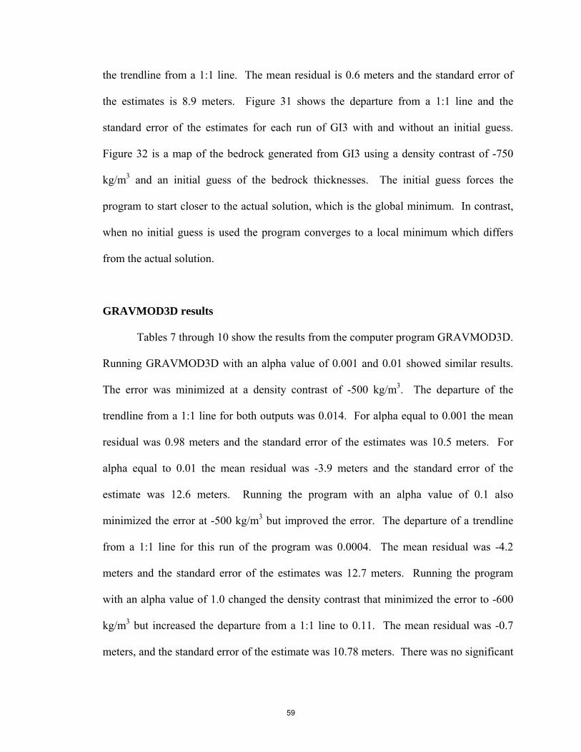
some statistics need to be employed. The depth to bedrock is known at various locations
throughout the survey area. By comparing the estimated depth to bedrock from the
computer programs to the known depth, one can calculate how well the estimate fits the
known data. Three sets of statistics were used to compare the known depths to the
calculated depths: the average residual, the fit of a data to a 1:1 line and the standard error
of the estimates. The average residual was found by subtracting the calculated depth
from the known depth at each location and then averaging those values throughout the
basin. This provides an estimate of how well the calculated depths match known depths,
but does not take into account the distribution of the data. High negative and high
positive residuals could average out to a near zero average residual. The fit of the
observations to a 1:1 line was then calculated by fitting a trendline to a plot of the known
depths versus calculated depths. If the calculated depths matched the known depths
exactly, the trendline would have a slope equal to 1. Comparing the difference in slope
of the trendline from 1 gives an estimate of how well the data fits. This method also does
not take into account the data distribution. The plot of known depths versus calculated
depths could have a large spread but still have a trend line with a slope close to 1. The
final statistic calculated is the standard error of the estimates. The standard error of the
estimates is the standard deviation of the difference between the calculated depth and the
known depth. This method takes into account the distribution of the data, the less scatter
the data has, the lower the stander error of the estimates will be. All of the statistics were
calculated using Microsoft Excel’s built in statistical functions.
52
GI3 Methods
Nyquest (2001) used the gravity inversion program GI3 [Cordell and Henderson,
1968] to invert the gravity data and estimate depths to bedrock. GI3 calculates the
gravitational effect of an array of vertical prisms, of assumed density contrast, to estimate
the gravitational signal of a basin. The initial guess at the thickness of each prism is
found by the infinite slab formula, which is a general equation used to calculate the
gravitational effect of an infinite horizontal sheet. The equation has the form of:
hGg ρπ2=Δ
Where:
gΔ is the gravity effect
G is the gravitational constant
ρ is the density of the slab
h is its thickness
Using the infinite slab formula, the gravity at each grid point is used to solve for
the thickness using the density contrast provided. Using the thickness found, the overall
gravitational attraction of the basin is found by summing the gravitational affect of each
prism over the basin. The gravity effect of each prism is found using the formula for a
vertical right-cylinder-source when the grid point coincides with the observation point
and the vertical-line-source for all other points. The calculated gravity is then compared
to the actual measured gravity and the thickness of each prism is adjusted based on the
difference between the two. This process continues iteratively until the error criteria are
met or the maximum number of iterations is performed. GI3 [Cordell and Henderson,
1968] does assume a constant density throughout the valley fill. The program also offers
53
the option to input an initial guess at the thickness of the sediment and the surface
topography of the basin. The program uses a fixed point iteration to iteratively find the
thickness of the basin. The formula for the fixed point iteration is:
⎟⎟⎠
⎞⎜⎜⎝
⎛=+ ),(
),(),(),(1 nmg
nmgnmznmz
calc
obskk
Where:
),(1 nmzk+ = new thickness at point ).( nm
),( nmzk = old thickness at point ).( nm
),( nmgobs = observed gravity at point ).( nm
),( nmgcalc = calculated gravity at point ).( nm
To determine the best use of GI3, I performed several experiments. The program
was run 20 different times with varying densities: 10 times with no initial guess or
surface topography and 10 times with an initial guess and surface topography. The
density contrasts used were: -400 kg/m3, -500 kg/m3, -600 kg/m3, -650 kg/m3, -700
kg/m3, -725 kg/m3, -750 kg/m3, -800 kg/m3, -900 kg/m3 and 1000 kg/m3. The input to
each run of the program consisted of a grid of the residual gravity anomaly and, when
necessary, grids of the surface topography and the initial thickness guess. Each grid had
a grid spacing of 50 meters. The initial guess was constructed from points of known
bedrock depths throughout the valley based on drill cores, wells and seismic data. The
output of each run of the program was a grid of points in the USGS grid format.
54
GRAVMOD3D Methods
I developed a second program to invert the gravity data based on code from
Chakravarthi and Sunderarajan (2004). GRAVMOD3D works in a similar fashion to
GI3 in that it calculates a theoretical gravitational attraction of a basin by summing the
effect from a series of prisms and iteratively corrects the thickness of the prisms by
comparing the calculated gravity to the actual gravity. This program uses Newton’s
forward difference formula to adjust the thickness of the model after each iteration. The
formula for Newton’s forward difference is:
( ))(2
),(),(),(.1 zG
nmgnmgnmznmz calcobs
kk ρπ Δ−
+=+
Where:
( )nmzk .1+ = new thickness at point ),( nm
),( nmzk = old thickness at point ),( nm
),( nmgobs = observed gravity of the basin at point ),( nm
),( nmgcalc = calculated gravity of the basin at point ),( nm
G = gravitational constant
)(zρΔ = density contrast at depth z
However, unlike GI3, GRAVMOD3D allows the density contrast to change with
depth. The program allows the density contrast to increase or decrease with depth along
a user defined parabolic curve. The parabolic curve is defined by the formula:
55
( )( )2
0
30
zz
αρρ
ρ−Δ
Δ=Δ
Where:
( )zρΔ = density at depth z
0ρΔ = density contrast at the surface
z = depth in kilometers
α = parabolic function constant alpha
The constant alpha allows the user to change the shape of the curve to match
geologic conditions. This program uses an analytical expression to calculate the gravity
of a three dimensional rectangle that was developed by Chakravarthi et al. (2002) which
takes into account the parabolic density function [Chakravarthi, et al., 2001;
Chakravarthi and Sundararajan, 2004, 2005].
I also modified the program to accept an initial guess at thickness. The residual
anomaly has to be input as an evenly-spaced grid of data points. The input file contains
the grid of points in rows and columns. The options contained in the input file are the
density contrast at the surface, the constant for the parabolic density function (alpha
value), grid dimensions and spacing, the maximum iterations to perform and the
maximum depth allowed. The maximum depth allowed is used to keep the iterative
process from calculating geologically unreasonable models. By constraining the
maximum depth the model is forced to conform to known or inferred maximum depths.
This keeps the model from using one or two anomalously deep cells to account for the
majority of the anomaly.
56
In order to determine which parameters resulted in the best fit to known depths,
this program was run 50 times with varying density contrasts and alpha values: 40 times
with no initial thickness guess and 10 times with an initial thickness guess. The 40 times
the program was run with no initial guess I used the same density contrasts as were used
in GI3. For each of the density contrasts the program was run with 4 different alpha
values: 0.001, 0.01, 0.1, and 1.0. The 10 times the program was run with an initial guess
the same density contrasts were used with an alpha value of 0.001. The input grid to the
program was a grid of the residual gravity with 250 meter grid spacing; thus, one expects
greater granularity in the result than with the GI3 spacing of 50 meters. This spacing was
chosen based on the detail retained and the computational time required to run the
program. The program was run 3 additional times with density contrasts of -725 kg/m3,
-500 kg/m3 and -400 kg/m3 with an alpha value of 0.001 and an input grid spacing of 50
meters to confirm the results found with the coarser grid spacing.
GI3 Results
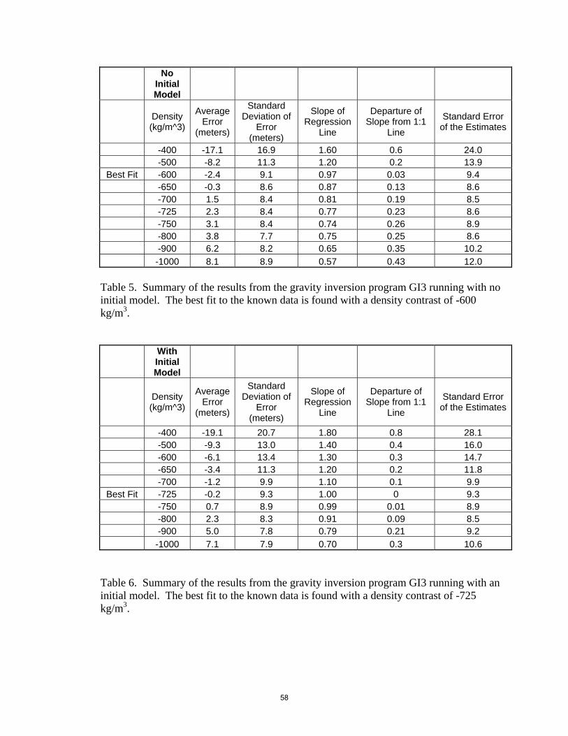
Tables 5 and 6 show the results from the computer program GI3. GI3, when
implemented with no initial guess, minimized the error between known depths and
calculated depths at a density contrast of -600 kg/m3. When known depths are plotted
versus calculated depths the departure of a linear trend line from a 1:1 line is 0.043. The
mean residual is -2.4 meters and the standard error of the estimates is 9.3 meters. When
an initial guess of the thickness was provided the density contrast that minimized the
error was found to be -750 kg/m3. The error associated with this value is 0.007 and is
found by again plotting known verse calculated depths and determining the departure of
Table 5. Summary of the results from the gravity inversion program GI3 running with no initial model. The best fit to the known data is found with a density contrast of -600 kg/mP
Table 6. Summary of the results from the gravity inversion program GI3 running with an initial model. The best fit to the known data is found with a density contrast of -725 kg/mP
3P.
58
the trendline from a 1:1 line. The mean residual is 0.6 meters and the standard error of
the estimates is 8.9 meters. Figure 31 shows the departure from a 1:1 line and the
standard error of the estimates for each run of GI3 with and without an initial guess.
Figure 32 is a map of the bedrock generated from GI3 using a density contrast of -750
kg/m3 and an initial guess of the bedrock thicknesses. The initial guess forces the
program to start closer to the actual solution, which is the global minimum. In contrast,
when no initial guess is used the program converges to a local minimum which differs
from the actual solution.
GRAVMOD3D results
Tables 7 through 10 show the results from the computer program GRAVMOD3D.
Running GRAVMOD3D with an alpha value of 0.001 and 0.01 showed similar results.
The error was minimized at a density contrast of -500 kg/m3. The departure of the
trendline from a 1:1 line for both outputs was 0.014. For alpha equal to 0.001 the mean
residual was 0.98 meters and the standard error of the estimates was 10.5 meters. For
alpha equal to 0.01 the mean residual was -3.9 meters and the standard error of the
estimate was 12.6 meters. Running the program with an alpha value of 0.1 also
minimized the error at -500 kg/m3 but improved the error. The departure of a trendline
from a 1:1 line for this run of the program was 0.0004. The mean residual was -4.2
meters and the standard error of the estimates was 12.7 meters. Running the program
with an alpha value of 1.0 changed the density contrast that minimized the error to -600
kg/m3 but increased the departure from a 1:1 line to 0.11. The mean residual was -0.7
meters, and the standard error of the estimate was 10.78 meters. There was no significant
59
Alpha =
0.001
Density (kg/m^3)
Average Error
(meters)
Standard Deviation of
Error (meters)
Slope of Regression
Line
Departure of Slope from
1:1 Line
Standard Error of the Estimates
-400 -11.5 15.8 1.29 0.3 19.5 Best Fit -500 -3.9 11.9 0.99 0.0 12.6
Table 7. Results from the gravity inversion program GRAVMOD3D. The inversion was run with an alpha value of 0.001. The best fit was found with a density contrast of -500 kg/m3.
Alpha =
0.01
Density (kg/m^3)
Average Error
(meters)
Standard Deviation of
Error (meters)
Slope of Regression
Line
Departure of Slope from
1:1 Line
Standard Error of the Estimates
-400 -11.6 15.8 1.29 0.3 19.6 Best Fit -500 -4.0 12.0 0.99 0.0 12.6
Table 8. Results from the gravity inversion program GRAVMOD3D. The inversion was run with an alpha value of 0.01. The best fit was found with a density contrast of -500 kg/m3.
60
Alpha =
0.1
Density (kg/m^3)
Average Error
(meters)
Standard Deviation of
Error (meters)
Slope of Regression
Line
Departure of Slope from
1:1 Line
Standard Error of the Estimates
-400 -12.2 16.2 1.33 0.3 20.3 Best Fit -500 -4.2 12.1 1.00 0.0 12.8
Table 9. Results from the gravity inversion program GRAVMOD3D. The inversion was run with an alpha value of 0.1. The best fit was found with a density contrast of -500 kg/m3.
Table 10. Results from the gravity inversion program GRAVMOD3D. The inversion was run with an alpha value of 1.0. The best fit was found with a density contrast of -600 kg/m3.
61
G
I3 N
o In
itial
Mod
el
0
0.1
0.2
0.3
0.4
0.5
0.6
0.7 40
050
060
070
080
090
010
00
Dens
ity C
ontr
ast x
-1 (k
g/m
3)
Departure from 1:1 Line
051015202530
Standard Error
GI3
With
Initi
al M
odel
0
0.1
0.2
0.3
0.4
0.5
0.6
0.7
0.8
0.9 40
050
060
070
080
090
010
00
Dens
ity C
ontr
ast x
-1 (k
g/m
3)
Departure from 1:1 Line
051015202530
Standard Error
Figu
re 3
1: G
raph
s sho
win
g th
e er
ror a
ssoc
iate
d w
ith th
e gr
avity
mod
elin
g pr
ogra
m G
I3 ru
n w
ith N
yque
st’s
(200
1) d
ata.
The
blu
e lin
e re
pres
ents
the
depa
rture
of t
he sl
ope
of a
tren
dlin
e fit
to th
e pl
ot o
f the
kno
wn
dept
hs to
bed
rock
ver
sus t
he c
alcu
late
d de
pths
to
bedr
ock.
The
mag
enta
line
repr
esen
ts th
e st
anda
rd e
rror
of t
he e
stim
ates
. Th
e gr
aph
on th
e le
ft sh
ow th
e re
sult
from
usi
ng G
I3 w
ith
no in
itial
gue
ss a
nd th
e gr
aph
on th
e rig
ht sh
ows t
he re
sults
from
usi
ng G
I3 w
ith a
n in
itial
gue
ss.
62
Fi
gure
32:
Fin
al m
odel
foun
d us
ing
the
grav
ity in
vers
ion
prog
ram
GI3
. Th
is is
the
mod
el th
at m
inim
ized
the
diff
eren
ce b
etw
een
the
calc
ulat
ed d
epth
and
kno
wn
dept
hs a
t var
ious
loca
tions
thro
ugho
ut th
e va
lley.
The
den
sity
con
trast
use
d w
as 7
50 k
g/m
3 .
63
change to the results by running GRAVMOD3D with an initial guess of the bedrock
depths. Figure 33 shows the departure from a 1:1 line and the standard error for each run
of GRAVMOD3D. Figure 34 is a map of the bedrock generated from GRAVMOD3D
using a density contrast of -500 kg/m3 and an alpha value of 0.1.
Comparison of GI3 and GRAVMOD3D
GRAVMOD3D minimizes the error at different density contrasts than GI3, which
is most likely a result of the algorithms used in each program. GRAVMOD3D is based
on code that was developed to model much larger basins than the Milltown Valley. It can
not handle the steeper gradients and small details associated with a small scale basin as
well as GI3 can. The difference in how the programs calculate thicknesses from the
calculated gravity causes the differences in the final models. Both programs compare the
calculated gravity to known gravity and make a correction to the thickness based on how
the two compare. GI3 finds the ratio between the observed gravity and the calculated
gravity and multiplies the old thickness by this ratio to find the new thickness.
GRAVMOD3D finds the difference between the observed gravity and calculated gravity
and uses the Bouguer Slab formula to calculate the thickness associated with the
difference in gravity and then adds that thickness to the old thickness to find the new
thickness. For example if there was a difference between the observed gravity and the
calculated gravity of 3 milligals, GI3 would multiply the old thickness by 4 to find the
new thickness, where as GRAVMOD3D would add approximately 100 meters to the old
thickness to find the new thickness. If the thickness was originally 50 meters the new
thickness for GI3 would be 200 meters and for GRAVMOD3D would be 150 meters.
64
GR
AVM
OD
3D A
lpha
= 0
.001
0
0.1
0.2
0.3
0.4
0.5
0.6 40
050
060
070
080
090
010
00
Den
sity
Con
trast
x-1
(kg/
m3)
Departure from 1:1 Line
0510152025
Standard Error
GR
AVM
OD
3D A
lpha
0.0
1
0
0.1
0.2
0.3
0.4
0.5
0.6 40
050
060
070
080
090
010
00
Den
sity
Con
trast
x-1
(kg/
m3)
Departure from 1:1 Line
0510152025
Standard Error
G
RAV
MO
D3D
Alp
ha 0
.1
-0.10
0.1
0.2
0.3
0.4
0.5
0.6 40
050
060
070
080
090
010
00
Den
sity
Con
trast
x-1
(kg/
m3)
Departure from 1:1 Line
0510152025
Standard Error
GR
AVM
OD
3D A
lpha
1.0
0
0.1
0.2
0.3
0.4
0.5
0.6 40
050
060
070
080
090
010
00
Den
sity
Con
tast
x-1
(kg/
m3)
Departure from 1:1 Line
051015202530
Standard Error
Figu
re 3
3: G
raph
s sho
win
g th
e er
ror f
or e
ach
run
of G
RA
VM
OD
3D.
The
blue
line
repr
esen
ts th
e de
partu
re fr
om th
e sl
ope
of a
1:1
lin
e fr
om a
tren
dlin
e fit
to th
e pl
ot o
f kno
wn
dept
hs to
bed
rock
ver
sus c
alcu
late
d de
pths
to b
edro
ck.
The
mag
enta
line
is th
e st
anda
rd
erro
r ass
ocia
ted
with
eac
h ru
n of
the
prog
ram
.
65
Fi
gure
34:
Fin
al d
epth
mod
el c
reat
ed w
ith th
e gr
avity
inve
rsio
n pr
ogra
m G
RA
VM
OD
3D.
This
is th
e m
odel
that
min
imiz
es th
e di
ffer
ence
bet
wee
n th
e ca
lcul
ated
dep
th a
nd th
e kn
own
dept
h at
var
ious
poi
nts t
hrou
ghou
t the
val
ley.
Thi
s dep
th m
odel
was
cre
ated
us
ing
a de
nsity
con
trast
of -
500
kg/m
3 and
a a
lpha
val
ue o
f 0.1
.
66
This shows how GI3 can assign more thickness to a single cell than GRAVMOD3D and
create steeper gradients. Figure 35 shows the final models from both GI3 and
GRAVMOD3D side by side. It is apparent that GRAVMOD3D creates a much smoother
map with broader features. This is even more apparent when you subtract the final model
created by GI3 from the final model created with GRAVMOD3D (Figure 36). The
biggest differences between the two occur around the deep “potholes” found throughout
the GI3 model. In these areas, the centers of the holes in GI3 have a deeper depth
estimate (15 to 40 meters). Around the edges of the holes GRAVMOD3D has a deeper
estimate (5 to 30 meters). GRAVMOD3D is creating the same gravitational response
with a broad hole which is overall deeper, but has a shallower maximum depth than the
holes created by GI3.
GRAVMOD3D more accurately matches the known depths to bedrock when
the density contrast is allowed to change very little with depth (alpha value = 0.1 or less).
The best fit to known depths using GRAVMOD3D was found with an alpha value of 0.1.
At the maximum depth extend found in the study area (≈ 150 meters) an alpha value of
0.1 results in a density contrast change of approximately 30 kg/m3 from the surface to the
deepest point. Increasing the alpha value causes the density contrast to change more
rapidly with depth (using alpha = 1.0 causes the density contrast to change by
approximately 500 kg/m3 from the surface to the deepest point). Increasing the alpha
value causes GRAVMOD3D to produce depth to bedrock models that do not match
known depths as well as it did with smaller alpha values. GI3 produces a model with the
best match to known depths and GRAVMOD3D does not improve significantly on GI3’s
model, especially when the density contrast decreases with depth. Based on these results
67
GI3 Final Bedrock Model
GRAVMOD3D Final Bedrock Model
Figure 35. Comparison between the best model found with GI3 and the best model found with GRAVMOD3D. You can see that the program GRAVMOD3D produces a much smoother model, omitting some of the detail seen on the GI3 model.
68
Fi
gure
36:
Map
show
ing
the
diff
eren
ce b
etw
een
the
final
dep
th m
odel
foun
d us
ing
GI3
and
the
final
dep
th m
odel
foun
d us
ing
GR
AV
MO
D3D
. Th
is w
as fo
und
by su
btra
ctin
g th
e fin
al m
odel
from
GI3
from
the
final
mod
el fr
om G
RA
VM
OD
3D.
It is
app
aren
t th
at G
RA
VM
OD
3D c
reat
es a
muc
h sm
ooth
er m
ap b
ut is
not
abl
e to
mat
ch th
e st
eep
grad
ient
s cre
ated
by
GI3
.
69
I am confident that the density contrast does not vary appreciably with depth. This is not
a big surprise for a narrow, fault bounded valley with a depth extent of less than 200
meters. And, from drilling results (Appendix A) we know there are local, steep gradients
on the bedrock surface. Therefore when incorporating the new data into the modeling I
used GI3.
2006 Addition of New Gravity Data to the Model
During the summer of 2006, Tony Bertholote collected an additional 204 gravity
measurements east of the previously collected data (Figure 37). This was done with the
intent to extend the bedrock model further to east along the Clark Fork River, to facilitate
a new groundwater model. Bertholote followed the same standard procedure as Nyquest
(2001) to reduce the gravity measurements to the Complete Bouguer Anomaly. Figure
38 shows the Complete Bouguer Anomaly including both the new and old data. This
new data and the previous data were combined into a larger data set, and following the
same methods outlined above, were inverted to find a depth to bedrock model. The new
depth to bedrock model includes all of the previous gravity data along with the new data,
extending the model up the Clark Fork and Blackfoot rivers.
Methods and Results
Since the new data were collected outside the extent of Nyquest’s (2001) area, the
regional field used to compute Nyquest’s (2001) residual gravity anomaly could not be
used, and a new regional gravity field had to be developed. The development of the
regional gravity field proved to be very difficult for this particular area due to a lack of
regional gravity data points near the valley and the shape of the valley itself. In order to
70
Figu
re 3
7. T
he lo
catio
ns o
f all
of th
e gr
avity
obs
erva
tions
incl
udin
g bo
th th
e da
ta c
olle
cted
in 2
001
and
the
data
col
lect
ed in
200
6.
The
new
dat
a ex
tend
s the
gra
vity
obs
erva
tions
up
the
Cla
rk F
ork
Riv
er a
nd u
p th
e B
lack
foot
rive
r.
71
Fi
gure
38:
Th
e co
mpl
ete
Bou
guer
ano
mal
y in
corp
orat
ing
all o
f the
dat
a, in
clud
ing
the
data
col
lect
ed in
200
1 by
Dav
e N
yque
st a
nd
the
data
col
lect
ed in
200
6 by
Ton
y B
erth
olot
e.
The
light
blu
e lin
e re
pres
ents
the
edge
of t
he v
alle
y an
d th
e da
ta u
sed
to c
onst
ruct
the
grid
are
show
n as
bla
ck d
ots.
72
constrain the gravity at the edge of the valley where no gravity measurements exist,
synthetic gravity points are created by digitizing points at the edge of the valley along the
contact of the bedrock with the valley fill. These points can be used constrain the gravity
anomaly because the anomaly must be zero at the edge of the valley. The gravity
anomaly is due to the material filling the valley being less dense than the bedrock
underneath. At the edge of the valley were the bedrock outcrops there is no less dense
material overlying the bedrock so we can assume the gravity anomaly along the edge of
the valley must be zero.
To find the gravity value at each digitized point the entire set of real gravity
points, including the regional and valley points are gridded. The gravity value at each
digitized point is assumed to be the value of the gridded gravity data at the location of the
digitized point. The digitized points are then added into the regional gravity data file and
force the residual anomaly to go to zero at the edge of the valley. Using this method the
regional gravity field was not able to produce a steep enough gradient in the residual
gravity anomaly at the edge of the valley and resulted in a residual anomaly that was less
than expected. Using this method, the gravity value at the digitized point is based on the
gridded surface of all of the known gravity. Assuming that at the valley edge there is a
relatively steep gravity gradient, I chose to add one milligal to the gravity value at each
edge point. This forces the regional gravity to produce a steep gradient at the edge of the
basin in the residual gravity anomaly.
Using the regional gravity data and the digitized valley edge points outlined above
a regional gravity field was produced. Figure 39 shows the regional gravity and the
points used to create it and Figure 40 show the regional gravity masked to the size of the
73
Fi
gure
39:
Th
e to
tal r
egio
nal g
ravi
ty u
sed
to c
reat
e th
e re
sidu
al g
ravi
ty a
nom
aly.
The
ligh
t blu
e re
ctan
gle
repr
esen
ts th
e ar
ea se
en in
th
e ot
her f
igur
es.
The
blac
k do
ts re
pres
ent a
ll of
the
data
use
d to
con
stru
ct th
e re
gion
al g
ravi
ty g
rid.
74
Fi
gure
40:
The
regi
onal
gra
vity
fiel
d us
ed to
find
the
resi
dual
ano
mal
y. T
he re
gion
al fi
eld
is a
n es
timat
e of
the
broa
d w
ave
leng
th
grav
ity re
spon
se in
the
area
. Th
e re
gion
al fi
eld
was
con
stru
cted
usi
ng d
ista
l poi
nts a
nd c
onst
rain
ed a
t the
val
ley
edge
. Th
e lig
ht b
lue
line
repr
esen
ts th
e ed
ge o
f the
val
ley
and
the
poin
ts u
sed
to c
onst
ruct
the
grid
are
show
n as
bla
ck d
ots.
Thi
s map
onl
y re
pres
ents
a
porti
on o
f the
tota
l reg
iona
l grid
cre
ated
. Se
e fig
ure
33 to
see
the
tota
l reg
iona
l gra
vity
use
d.
75
valley. Separating the regional gravity from the total gravity produced a residual gravity
anomaly that was similar to the previous work (Figure 41) by Nyquest (2001) where they
overlap. The residual anomaly was inverted using GI3 following the same steps given in
the previous section. The end result was a best fit to known depths to bedrock using a
density contrast of -500 kg/m3. The departure of the slope of a trend line fitted to the plot
of the 173 known depths to bedrock versus the calculated depths to bedrock is 0.11. The
mean residual is -1.9 meters and the standard error of the estimates is 15 meters. Figure
42 shows the departure of the trend line from a 1:1 line and the standard error for each
run of GI3 with the complete data set. The details of the gravity data processing can be
seen in Appendix D including the specific gridding parameters used to develop the grids.
Conclusion
Nyquest (2001), using the smaller data set, found the modeled depths matched the
known depths best at a density contrast of -750 kg/m3, which does not match my results
based on the larger data set. GI3 was the only computer model that minimized the error
at -750 kg/m3 using Nyquest’s data along with an initial guess at the thickness. All other
computer models generated using both GI3 and GRAVMOD3D minimize the error at
-500 kg/m3 or -600 kg/m3. In order to try and replicate the results found by Nyquest
(2001), an initial guess identical to the initial guess used by Nyquest (2001) was created
to use in GI3. In the areas outside of Nyquest’s (2001) study area where no initial guess
yet existed, a simple function was used to estimate the depth to bedrock based on the
gravity. By dividing the known depths by their associated gravity response, a constant
value of -40 m/mgal was found. Therefore, an initial guess could be calculated by
multiplying the gravity at the locations where no initial guess existed by -40 m/mgal.
76
Fi
gure
41:
The
resi
dual
ano
mal
y fo
und
by su
btra
ctin
g th
e re
gion
al re
spon
se fr
om th
e to
tal C
BA
. Th
e re
sidu
al a
nom
aly
has a
val
ue o
f ze
ro a
long
the
valle
y ed
ge a
nd is
neg
ativ
e in
side
the
valle
y. T
he li
ght b
lue
line
repr
esen
t the
edg
e of
the
valle
y an
d th
e bl
ack
dots
re
pres
ent t
he d
ata
used
to c
onst
ruct
the
grid
.
77
GI3
All
Dat
a
0
0.51
1.52
2.53
3.54 10
020
030
040
050
060
070
080
090
010
00
Den
sity
Con
trast
x-1
(kg/
m3)
Departure from 1:1 Line
020406080100
120
140
Standard Error
Fi
gure
42:
Plo
t of t
he d
epar
ture
of t
he sl
ope
of a
tren
dlin
e (in
blu
e) fi
tted
to th
e pl
ot o
f the
kno
wn
dept
hs to
bed
rock
ver
sus t
he
calc
ulat
ed d
epth
s to
bedr
ock
from
a 1
:1 li
ne a
nd th
e st
anda
rd e
rror
(in
mag
enta
) of e
ach
run
usin
g G
I3 w
ith th
e co
mpl
ete
data
set.
78
Using GI3 with the complete data set and the same initial guess used as Nyquest (2001)
for his area also produced a model that minimized the errors at -500 kg/m3.
Based on the evidence generated by the different computer models and on the
data collected by Evans (1997), who found the range of density contrasts in the area to be
between -250 and -740 kg/m3, I believe that the density contrast of -500 kg/m3 is the best
approximation for the Milltown valley area. With the incorporation of the new gravity
data the survey area covers a larger area, where the make up and compaction of the
alluvium filling the valley may be different. With the larger area it is not unreasonable to
assume the average density contrast across the survey area may be different than the
average density contrast for the smaller area. A density contrast of -500 kg/m3 is the
minimum possible density contrast that preserves the short wavelength features seen in
the residual anomaly and reasonably matches the known depth to bedrock. Decreasing
the density contrast between the valley fill and the bedrock causes the depth to bedrock to
be too deep and loses the short wavelength features. Increasing the density contrast
causes the modeled depth to bedrock to be too shallow. For example, using a density
contrast of -100 kg/m3 produces a model that has a mean residual of -100 meters,
meaning the depths calculated are on average 100 meters too deep. Using a density
contrast of -1000 kg/m3 produces a model with a mean residual of 11 meters, meaning on
average the depths are 11 meters to shallow. Figure 43 shows examples of how the
density contrast affects the estimates of bedrock depth.
Table 11 shows the results from using GI3 with the complete data set and Figure
44 shows the final depth to bedrock model generated from all the current gravity data and
is constrained by all available depth to bedrock control data. The error in the depth
79
Density (kg/m^3)
Average Error
(meters)
Standard Deviation of
Error (meters)
Slope of Regression
Line
Departure of Slope from 1:1
Line
Standard Error of the Estimates
-400 -8.5 16.7 1.12 0.1 18.7 Best Fit -500 -1.9 15.0 0.89 0.1 15.0
Table 11. Results from the gravity inversion program GI3 using all of the current data. The best fit to the known depths was found using a density contrast of -500 kg/m3.
80
Known vs. Calculated Depths (density contrast -100 kg/m3)
y = 4.4609x
0
50
100
150
200
250
300
350
400
0 10 20 30 40 50 60 70 8
Known Depths (m)
Calc
ulat
ed D
epth
s (m
)
0
Known vs. Calculated Depths (density contrast -1000 kg/m3)
y = 0.4461x
0
10
20
30
40
50
60
70
80
0 10 20 30 40 50 60 70 8
Known Depths (m)
Calc
ulat
ed D
epth
s (m
)
0
Figure 43: The two charts show the calculated depths verses the actual depths for two different density contrasts. The black line is the trend line fit to the data. The red line is a 1:1 line which represents a perfect fit between known depths and calculated depths. The top graph’s calculated depths were found using a small density contrast (-0.1 g/cc) and the bottom graph’s calculated depths were found using a large density contrast (1 g/cc). Using the small density contrast the depths are over estimated and using the large density contrast the depths are underestimated.
81
Fi
gure
44:
Fin
al d
epth
mod
el fo
r the
ent
ire fi
eld
area
. Th
is is
the
mod
el th
at m
inim
izes
the
erro
r bet
wee
n kn
own
dept
hs th
roug
hout
th
e va
lley
and
the
calc
ulat
ed d
epth
s fou
nd u
sing
GI3
. T
his m
odel
incl
udes
surf
ace
topo
grap
hy a
nd a
n in
itial
gue
ss a
s inp
uts i
nto
GI3
. Th
e de
nsity
con
trast
ed u
sed
to c
onst
ruct
this
mod
el is
-500
kg/
m3 .
82
estimates found using gravity methods comes from the errors associated with collecting
gravity data, undetected lateral/vertical changes in density contrast, and possible
insufficient observations in areas of steep bedrock gradient. Nyquest (2001) stated a total
error associated with his measurements to be 0.15 mgal. Assuming all data used to
construct the final model is as accurate as the data collected by Nyquest (2001), then the
final model has a standard error of ±15 meters.
As an additional check of the final bedrock model I choose to use the depths
calculated by the inversion in a forward model. Forward modeling calculates the
gravitational response expected from a particular basin geometry, as opposed to inverse
modeling which calculates a basin geometry from a measured gravitational response.
Using the thickness model generated by GI3 as an input into GI3’s forward modeling
module, the expected gravitational response can be calculated (Figure 45). Directly
comparing the measured gravitational response to the gravitational response found by
forward modeling (Figure 46) shows that the two differ very little across the survey area.
For most of the valley the difference between the two is very close to zero and the
maximum difference is less than 0.001 mgals.
The residual error for the final map (Figure 44) is found by comparing known
depths to bedrock at various locations throughout the study area to the calculated depth at
the same location. If the density contrast really is constant throughout the survey area
then the value of the residuals should be completely random, i.e. an even distribution of
positives and negatives with no dependence on location. However, the map showing the
distribution of the residuals (Figure 47) does not confirm this. The map shows a strong
dependence on location as to whether the residual is positive or negative. In Hellgate
83
Figu
re 4
5: G
ravi
ty a
nom
aly
crea
ted
by fo
rwar
d m
odel
ing
the
calc
ulat
ed d
epth
s to
bedr
ock.
Thi
s is t
he e
xpec
ted
grav
ity a
nom
aly
with
th
e be
droc
k co
nfig
urat
ion
seen
in F
igur
e 44
.
84
Figu
re 4
6: D
iffer
ence
bet
wee
n th
e m
easu
red
grav
ity a
nom
aly
and
the
grav
ity a
nom
aly
calc
ulat
ed b
y fo
rwar
d m
odel
ing
the
bedr
ock
conf
igur
atio
n se
en in
Fig
ure
44.
85
Figu
re 4
7: D
istri
butio
n of
the
erro
rs in
the
stud
y ar
ea.
The
resi
dual
s wer
e fo
und
by su
btra
ctin
g th
e ca
lcul
ated
dep
th to
bed
rock
from
th
e ac
tual
dep
th to
bed
rock
. Neg
ativ
e va
lues
for t
he re
sidu
al re
pres
ent t
he m
odel
ove
r est
imat
ing
the
dept
h an
d po
sitiv
e re
sidu
als
repr
esen
t the
mod
el u
nder
estim
atin
g th
e de
pth.
86
Canyon the residuals are all positive, which means the model is underestimating the
actual depth. Just to the east of the Milltown Dam the residuals are all negative, which
means the model is overestimating the depths. In both areas the local geology is affecting
the modeled results. In Hellgate Canyon, fault zones nearby causes the bedrock to be less
dense than the surrounding rock [J. Sears, personal communication, May 2007], which
decreases the density contrast between the valley fill and the bedrock. This causes my
selection of a density contrast to be too great for the area and underestimates the depth.
A similar problem is found in the area east of Milltown Dam. An igneous sill, which is
denser than the surrounding bedrock, has been mapped in that location [J. Sears, personal
communication, May 2007]. The igneous sill is a local high density area in the bedrock,
such sills have densities as high as 3200 kg/m3 [Sheriff, personal communication, May
2007]. Above this high density bedrock, there will be a corresponding high in the
complete (and residual) Bouguer anomalies. Modeling (or inverting) the gravity using a
constant density contrast for the valley fill will result in an artificial bedrock high in the
area over the higher density sill, because less low density fill is required to explain the
locally higher gravity. Consequently, one must keep in mind that the estimate presented
in Figure 44 assumes constant density bedrock across the whole area. For example, a 50
meter thick sill of density contrast + 200 kg/m3 across half the Milltown Valley would
add approximately 0.5 mgals to the anomaly resulting in an artificial high on the order of
25 meters. Undoubtedly, there are local variations in the bedrock density, and the region
of Figure 47 with concentrated negative residual overlies the projection of the sill into the
subsurface.
87
Comparing Nyquest’s (2001) map to the map I constructed shows several
differences. Subtracting Nyquest’s (2001) map from the map I constructed (Figure 48)
highlights these differences. On average my map is deeper than Nyquest’s (2001) map,
but there are areas where mine is shallower despite both maps being generated from
similar gravity anomalies. The largest differences occur in areas where the gravity
measurements are sparse or in areas that were boundaries in Nyquest’s (2001) map and
are not in mine. I was unable to recover Nyquest’s exact methods for developing his
residual gravity anomaly; i.e. what data he used and what data he threw out, his gridding
parameters, etc; which could account for the differences between his final map and my
final map. My final map (Figure 44) incorporates a larger gravity data set and covers
more area, and represents the current best estimate for depth to bedrock in the greater
Milltown area. All of the gravity data available to me along with my seismic data and
previous depth to bedrock information (Appendix A) were used to construct this estimate.
88
Figu
re 4
8: D
iffer
ence
map
bet
wee
n th
e pr
evio
us m
ap a
nd th
e ne
w m
ap I
crea
ted
whe
re th
e tw
o co
inci
de.
The
map
I cr
eate
d w
as
subt
ract
ed fr
om th
e pr
evio
us m
ap.
Posi
tive
valu
es re
pres
ent w
here
the
new
map
is d
eepe
r and
neg
ativ
e va
lues
repr
esen
t whe
re th
e ne
w m
ap is
shal
low
er.
The
whi
te d
ots s
how
the
loca
tion
of th
e gr
avity
mea
sure
men
ts.
89
COMPARISON OF SEISMIC REFLECTION AND GRAVITY METHODS
The combination of previous seismic results, gravity observations and wells to
bedrock, when combined with new reflection seismology and an extended gravity
interpretation provides a more extensive map of bedrock topography. The combined data
provide a better constrained solution for the bedrock topography in the greater East
Missoula Area.
Comparing the seismic data to the gravity data shows a reasonable correlation
between the two. The depth estimates from the seismic data match the depth estimates
from the gravity at similar locations. Both of the estimates are also similar to known
depths to bedrock from well log and drill core data. All three methods, seismic, gravity
and well log and drill core data, have inherent errors associated with them. The seismic
data depends heavily on the velocity of the layers and on the interpreter’s ability to pick
reflections. The gravity data depends heavily on the density contrasts and the regional-
residual separation. The well logs and drill core data have many ambiguities in them
which are a direct result of the process (i.e. did the drill go into a large boulder of bedrock
or did it actually hit the bedrock? Did the driller get paid by the foot?). For each depth
estimate there is a standard error of at least ± 5 meters.
The velocity analysis of the seismic data at each location does provide some
insight into how the density of the valley fill varies in the valley. In a broad sense, the
velocity of a material increases with an increase in density of the material. If the density
of the valley fill increased in the vertical direction I would expect to see gradual increase
in the velocity. If this were the case, the first arrivals in the seismic section would lie
along a curved line. In the seismic data collected the first arrivals lie along a straight line
90
that fits those arrivals with a R2 value of 0.98 or greater. This supports the conclusion
found in the gravity section above that the density of the valley fill does not increase
significantly with depth. Looking at the lateral variations in the velocity of the valley fill
suggests that the density of the valley fill may change latterly in the valley. The velocity
of the valley fill was the greatest in Hellgate Canyon, suggesting that the density of the
valley fill was higher. This could account for the gravity model underestimating the
depths in this area. If the density of the valley fill were higher, there would be less
density contrast in that area between the valley fill and the bedrock. The model would be
using too high of a density contrast in that area, which would result in an underestimation
of the depth. The opposite is true along Deer Creek Road. This area has the slowest
velocity of the valley fill, which suggests that the density of the valley fill in this area is
less dense. Here the model overestimates the depth because it is using too low of a
density contrast. The velocity found from seismic methods could be a good indicator of
how the density of the valley fill varies in a lateral direction.
91
CONCLUSION
Seismic reflection methods can be used to improve the bedrock map in the study
area, although it only works well in areas that are shallower than 40 meters. The best use
of seismic in this area would be to provide more data for comparison between the depths
found using gravity inversion and depths from other methods (seismic, drill cores and
wells) or to further resolve the depth to bedrock in areas where the gravity gradient is
high. Another use of seismic methods would be to determine lateral variations in the
density of the valley fill through the use of velocity analysis. Performing additional
seismic in the area may be difficult though due to land access issues and environmental
factors. In order to perform a seismic survey in the study area a source capable of putting
a large amount of energy into the ground is needed due to the high attenuation of the
alluvium. It would also be expensive to perform a large scale seismic survey in this area
(3 to 4 people plus equipment for the seismic versus 1 to 2 people with a gravimeter for a
gravity survey).
The seismic reflection data is useful for building a general model of the bedrock,
but for modeling the entire basin gravity methods are still the method of choice.
Interpreting the gravity data into a depth model is best done with GI3. This computer
program has no problem dealing with the small scale of the basin and the high gradients
in the anomaly. Also analysis of both the gravity data and seismic data suggest that the
density of the valley fill remains constant in the vertical direction, so there is no need to
model the gravity data with a program that allows the density contrast to change with
depth. Nyquest’s (2001) map produced using gravity inversion shows the most detail of
the maps that were available at the beginning of this study and was a considerable
92
improvement to Gestring’s (1994) map. Using 598 gravity measurements, ten new
seismic reflection lines and data from drill cores, wells completed to bedrock and
previous seismic refraction data I constructed a new map. The new map is based heavily
on the gravity data and is constrained with the seismic reflection data, drill cores, wells
completed to bedrock and the previous seismic refraction data. The seismic reflection
data, drill cores, wells completed to bedrock and previous seismic refraction data was
used to create an initial bedrock model as a starting point for the gravity inversion and to
provide an estimate of how well the gravity inversion fit actual depths.
Using the complete gravity data set the computer modeling converges to the same
solution regardless of the initial model. Using the additional seismic data, along with the
other known depths to bedrock data to construct an initial model the modeling program
converges to the same final model as it did without an initial guess. The collection of
seismic data in a situation like this can be used to better constrain the final model by
having additional depth data to compare the solution to. This would allow a better
understanding of the error associated with the final model and ways to minimize the error
further.
The additional gravity data collected, when integrated with the previous data,
greatly increased the coverage of the bedrock model. The new data proved difficult to
incorporate and model, raising some new problems that had to be overcome. After
processing and inverting the combined gravity set, a new bedrock model was created.
Additional work that could be done would include the collection of more seismic data to
further refine the final model output by GI3. Additional gravity data could also be
collected in the study area and in the surrounding areas. The new gravity data set covers
93
a much bigger area than before but still has portions that need more gravity
measurements. Filling in these areas and collecting a series of regional gravity points in
the area directly surrounding the valley could greatly improve on the accuracy of the
bedrock model.
With the data collected to date, Figure 44 shows the best estimate of the bedrock
topography of the Milltown Valley and surrounding area. The map differs from
Nyquest’s (2001) map in various locations but still provides a geologically reasonable
solution. The model incorporates all of the current gravity data and is constrained by
depths from drill cores, wells completed to bedrock and seismic refraction and reflection
data.
94
REFRENCES Associates, H. L. (1987), Volume 1, Milltown Reservoir Data Report Supplemental Investigations Conducted Under the Feasibility Study., Harding Lawson Associates, Denver, Colorado, HLA Job No. 17461,002.10. Barbosa, V. C. F., et al. (1999), Stable inversion of gravity anomalies of sedimentry basins with nonsmooth basement reliefs and arbitrary density contrasts variations, Geophysics, 64, 754-764. Bear, G. W., et al. (1995), Linear inversion of gravity data for 3-D density distributions Geophysics, 60, 1354-1364. Blackhawk Geosciences, I. (1990), Seismic Refraction Survey, Milltown Reservoir Sediments Site, 6-7 pp, Misoula, MT. Bradford, J. H. (2002), Depth characterization of shallow aquifers with seismic reflection Part 1 - The failure of NMO velocity analysis and quantative error prediction, Geophysics, 67, 89-97. Camacho, A. G., et al. (2000), Gravity inversion by means of growing bodies, Geophysics, 65, 95-101. Camp, D., and McKee (1989), Milltown Downstream Screening Study: Data Report. Chai, Y., and W. J. Hinze (1988), Gravity inversion of an interface above which the density contrast varies exponentially with depth, Geophysics, 56, 837-845. Chakravarthi, V., et al. (2001), INVER2DBASE - A program to compute basement depths of density interfaces above which the density contrast varies with depth, Computers and Geosciences, 27, 1127-1133. Chakravarthi, V., and N. Sundararajan (2004), Automatic 3-D gravity modeling of sedimentary basins with density contrast varying parabolically with depth, Computers and Geosciences, 30, 601-607. Chakravarthi, V., and N. Sundararajan (2005), Gravity modeling of 2 1/2-D sedimentary basins -- a case of variable density contrasts, Computers and Geosciences, 31, 820-827. Cordell, L., and R. G. Henderson (1968), Iterative three-dimensional solution of gravity anomaly data using a digital computer Geophysics, 33, 596-601. Evans, C. (1997), A Gravity Interpretation of the Bedrock Structure of the Central Missoula Valley, Montana, University of Montana Missoula, Montana
95
Garcia-Abdeslem, J. (2003), 2D modeling and inversion of gravity data using density contrast varying with depth and source - basement geometry described by the Fourier series, Geophysics, 68, 1909-1916. Garcia-Abdeslem, J. (2005), The gravitational attraction of a right rectangular prism with density varying with depth following a cubicv polynomial, Geophysics, 70, j39-j42. Gestring, S. (1994), Interaction of the Clark Fork River with the,, University of Montana, Missoula, Montana. Goforth, T., and C. Hayward (1992), Seismic reflection investigations of a bedrock surface buried under alluvium, Geophysics, 57, 1217-1227. Guspi, F. (1992), Three-dimensional Fourier gravity inversion with arbitrary density contrast, Geophysics, 57, 131-135. Lankston, R. W. (1988), High resolution refraction data acquistition and interpretation, in Symposium on the Application of geophysics to engineering and environmental problems, edited, Golden, CO. Li, Y., and D. W. Oldenburg (1998), 3-D inversion of gravity data, Geophysics, 63, 109-119. Mendonca, C. A. (2004), Inversion of gravity-field inclination to map the basement relief of sedimentray basins, Geophysics, 69, 1240-1251 Nelson, W. H., and J. P. Dobell (1961), Geology of the Bonner Quadrangle, Montana, U.S. Geological Survey Bull. 1111-F, 235 Nyquest, D. (2001), A Depth to bedrock model of the hellgate canyon and bandmann flats area, East Missoula, Montana using constrained inversion of gravity data, Masters thesis, 186 pp, University of Montana, Missoula. Pullan, S. E., and J. A. Hunter (1991), Delineation of buried bedrock valleys using the optimum offset shallow seismic reflection technique, Investigations in Geophysics 5, 75-87. Rene, R. M. (1986), Gravity inversion using open, reject, and "shape-of-anomaly" fill criteria, Geophysics, 51, 988-994. Reynolds, J. M. (1997), An Introduction to Applied and Environmental Geophysics, 796 pp., John Wiley & Sons, Chichester. Salem, A., et al. (2004), Lineraized least-squares method for interpretation of potential-field data from sources of simple geometry, Geophysics, 69, 783-788
96
Silva, J. B. C., et al. (2000), Gravity inversion using convexity constraint, Geophysics, 65, 102-112. Steeples, D. W., and R. D. Miller (1991), Seismic reflection methods applied to engineering, environmental, and groundwater problems, Investigations in Geophysics, 5, 1-30. Steeples, D. W., and R. D. Miller (1998), Avoiding pitfalls in shallow seismic reflection surveys, Geophysics, 63, 1213-1224. Thompson, M. D., McGinnis, L. D., Wilkey, P. L., Miller, S. F. (1997), Gas Rich Sediment and Cosatal Wetland Loss in Louisiana, Open Source Report: Argonne National Labratory. Treitel, S., and L. Lines (2001), Past, present, and future of geophysical inversion - A new millennium analysis, Geophysics, 66, 21-24. Woessner, W. W. (1988), Missoula Valley Aquifer Study: Hydrogeology of the Eastern Portion of the Missoula Valley Aquifer, Missoula County, Montana, Helena, Montana. Woessner, W. W. (1993), Clark Fork natural Resource Damage Assessment. Milltown Ground water Injury Report, University of Montana, Missoula, Montana. Woessner, W. W., et al. (1984), Arsenic Source and Water Supply Remediation Action Study, Milltown Montana. Woessner, W. W., and W. A. Popoff (1982), Hydrogeologic Survey of Milltown, Montana and Vicinity, Helena, Montana. Xu, S.-z., et al. (2003), A new method for continuation of 3D potential fields to a horizontal plane, Geophysics, 68, 1917-1921.
97
APPENDIX A
EMC Depths ID State Plane X (m) State Plane Y (m) Thickness (m)
APPENDIX B Bonner School Field Seismic Lines GPS Coordinates of first geophone Line 1: 281198 mE 5194337 mN Line2: 281256 mE 5294379 mN Line Direction Line1: N35E Line 2: N50E Deer Creek Road Seismic Lines GPS Coordintates of first Geophone Line 1: 278262 mE 5195258 mN Line 2: 278173 mE 5195358 mN Line 3: 278170 mE 5195364 mN Line 4: 278043 mE 5195509 mN Line 5: 277781 mE 5195836 mN Line Directions All lines were run parallel to Deer Creek Road Hellgate Canyon Park Seismic Lines GPS Coordinates of the first Geophone Line1: 274263 mE 5193964 mN Line 2: 274262 mE 5193952 mN Line 3: 274261 mE 5193928 mN Line Directions All Lines were run parallel to Highway 200 See data CD for raw field data
102
APPENDIX C
• Field data was stored in the onboard memory of the Smartseis until it could be transferred to a PC in the lab using a serial cable.
• Data was sorted into site specific folders and backed up in multiple locations
• The file names assigned by the Smartseis had to be changed from the numeric
naming convention used by the Smartseis to an alpha-numeric scheme. Names were chosen based on the location and number of the shot at the location
• The individual Smartseis files were combined into a single Seismic Unix file
using a demonstration version of Seismic Unix NT.
• Seismic Unix NT was used to calculated the offset and midpoint of each shot and write the values to the Seismic Unix file.
• The files were analyzed visually to determine the optimum offset for each
location.
• All remaining steps were completed using seismic unix running on a Linux based computer system.
• The traces corresponding to the optimum offset were extracted using the suwind
command and placed in a new file.
• The new file was filtered and gained to produce the final sections
o Filter Settings: Sufilter was used to filter the data using the bandpass settings. The filter tapered from 30 Hz up to 45 Hz and down from 120 Hz to 175 Hz.
o Gain Settings: Sugain was used to gain the filter using automatic gain control. The agc window was set to 0.09 seconds.
103
APPENDIX D
• Starting with the gravity data reduced to the CBA
• The gravity data was separated into two separate files, one containing all of the gravity points and one containing just the gravity points to be used for the regional.
• Using a geo-referenced topo map the edge of the valley was digitized
• The file containing all of the gravity points was gridded in Surfer using the
minimum curvature method with a grid spacing of 75 meters and the default options (see below). This created the total CBA grid.
• The value of the total CBA grid was extracted at each point of the digitized valley
edge.
• A constant was added to the value of the CBA at each digitized edge point (1 mgal) in order to create the gravity gradient at the edge of the valley
• The digitized edge points with the value of the CBA plus the constant were added
to the file containing just the regional gravity points.
• The regional gravity points, including the digitized edge points were gridded in Surfer using the same settings used to created the total CBA grid. This created the regional gravity grid.
• The regional gravity grid was subtracted from total CBA grid to create the
residual anomaly grid.
• The residual anomaly grid was trimmed and cleaned up to be used as an input to the gravity inversion programs.
Note: The above outlined steps are an iterative process that may need to be completed several times in order to achieve acceptable results. Editing of the gravity data by adding or removing points may be necessary.
• After inverting the gravity data using an inversion program the output files from the programs are converted to Surfer grids.
• The value of the output grid is extracted at each location of a known depth.
• Statistical analysis is done to compare the known depth to the calculated depth
and determine the error in the depth estimate.
104
Surfer Grid Settings • Minimum curvature method
o Max Residual = 0.039 o Max Iteration = 10,000 o Relaxation Factor = 1 o Internal Tension = 0 o Boundary Tension = 0 o Anisotropy Ration = 1
105
APPENDIX E
Seismic Source: Bison Industries Elastic Wave Generator Approximately 100 Kg hammer Hydraulic Control Seismic Data Aquistion: Geometrics Smartseis Number of Channels: 24. Sample Interval: 31, 64, 125, 250, 500, 1000 or 2000 μs. Record Length: up to 16,000 samples per channel. Acquisition Filters and Noise Reduction Technology: Many field sites are noisy – moving vehicles, overhead power lines, vibrating machinery. The SmartSeis includes real-time digital filters that you can customize to improve your data in adverse urban environments. • 32 –bit Stacking: Reduces contributions from random noise by letting you add repeated hammer blows to improve signal strength. • Memory Freeze: Allows selective stacking of weak channels. • Power Line Notch: Reduces 50/60 Hz and harmonics. • Low-Cut Filtering: Reduces the effects of distant traffic and ground roll. Includes filter frequencies of out, 25, 35, 50, 70, 100, 140, 200, 280, 400 Hz. • High-Cut Filtering: Removes wind noise. Includes filter frequencies of out, 250, 500, 1000 Hz. • Display Filters can be run non-destructively after raw data is collected, making costly repeated shots unnecessary. Custom filter frequencies are available. Display: High-resolution 640x480 LCD, PC compatible. Visible in bright sunlight. Noise Monitor: Waterfall style moving trace display, also shows channel continuity and geophone performance. A/D Conversion: 20-bit result, 32-bit stacker. Gain Control: Automatic, set by continuously measuring two-stage instantaneous floating-point amplifier. True amplitude is preserved and can be used for ground motion studies. • Fault Location • Stratigraphic mapping • Gravel and aggregate mining • Thickness of overburden • Mineral and gold exploration • Landfill delineation and siting • IBC Vs30 site classification Data Display: Wiggle-trace, shaded or variable area, trace clipping, automatic gain control, fixed gain and post-acquisition
106
filtering included. Energy Sources: Hammer, weight drop or explosives. Pretrigger: Allows viewing of data before trigger. Delay: 0 to 9999 ms in 1 ms increments. Data Storage: Sufficient for several days recording. Includes both floppy and hard drive storage. In-field Processing: • Automatic first break picking with manual over-ride. • On-screen travel time plots. • Automatic layer assignments with manual over-ride • Automatic calculation of depths below shots and geophones. Built-in software ray traces model and indicates where data quality might be poor. Prints table of all data, depth calculations and a quality control plot showing questionable data. Report-ready cross section annotated with calculated velocities. Analysis and interpretation software from Rimrock Geophysics. PCbased packages also available. Please contact the factory. Interfaces: RS-232, video, keyboard and printer. Data Format: SEG-2 standard. Mating Connectors: Cannon NK-27-21C, 12 channels each connector. Plotter: Built-in four-inch (11 cm) wide thermal printer. Testing: Full instrument testing available using Geometrics external test oscillator system. Power: Runs on 12V auto-type battery. GPS Location: Garmin GPSMAP 60C 12 channel parallel GPS receiver Gravity Meter: Scintrex Model CG3 Sensor Type Fused Quartz using electrostatic nulling Reading Resolution 5 µgal Standard Deviation: <10 µgal Operating Range 8,000 mgal, without resetting Residual Long-term Drift (static) Less than 0.02 mgal/day Range of Automatic Tilt Compensation ±200 arc sec. Tares Typically less than 5µgal for a 20g shock Automated Corrections Tide, Instrument Tilt, Temperature, Noisy Reading Rejection Dimensions 240 mm x 310 mm x 320 mm 9.4" x 12.2" x 12.6" Weight (including battery) 11.0 kg (24.2 lbs) Power Consumption 4.5 watts at 25 C
107
Operating Temperature -40 C to +45 C (optional ranges available) Memory 48k RAM, suitable for up to 1200 readings Real Time Clock Internal provides day, month, year, hours, minutes, seconds Digital Data Output RS-232C serial interface