Seismic velocity inversion for patchy and homogeneous fluid-distributionconditions in shallow, unconsolidated sands
Jie Shen1 and Juan M. Lorenzo2
ABSTRACT
Knowledge of homogeneous and heterogeneous fluid-distri-bution conditions in unconsolidated sediments is important forthe selection of remediation techniques for groundwater con-tamination. However, for unconsolidated sediments, fluid-distri-bution conditions from laboratory tests on core samples may notbe representative of in situ conditions. We have developed aseismic inversion method to determine in situ fluid-distributionconditions that involves inverting experimental seismic P- andS-wave velocities using Hertz-Mindlin and Biot-Gassmannmodels with different averaging methods (Wood and Hill aver-ages) and different fluid-distribution condition assumptions.This method can determine whether seismic velocity-versus-
depth profiles are better explained assuming heterogeneous orhomogeneous saturation conditions in shallow (<1 m depth)unconsolidated sands. During the imbibition and drainage ofshallow unconsolidated sands, we have observed nonmonotonicrelationships between P-wave velocity and water levels (WLs)as well as an S-wave velocity and WLs that were consistentwith other field and laboratory observations. This relationshipcan be explained by transitions between the lower Wood boundand the higher Hill bound. The transition is possibly causedby the alternation in the size of fluid patches between smalland large during the imbibition and drainage. Inverted resultscan be verified by a good correlation (difference <7%) betweenthe inverted and measured water saturation using moisturesensors.
INTRODUCTION
Partially saturated unconsolidated sediments contain a mixture oftwo or more fluids that can be distributed either homogeneously orheterogeneously (in patches). However, the commonly applied lab-oratory ultrasonic core tests for identifying fluid distributions arecostly and may not represent in situ conditions because of the dis-turbance of unconsolidated samples during core transportation, andthe scaling issues with translating between ultrahigh frequenciescommonly used in laboratory studies and lower frequencies usedin the field (Cadoret et al., 1995; Toms-Stewart et al., 2009). Duringfield tidal water-level (WL) change experiments (Bachrach and Nur,1998) and laboratory WL change experiments (Velea et al., 2000;Lorenzo et al., 2013), changes in WL and water saturation Sw leadto unexpected alternations of the fast P-wave velocity VP betweenincreasing and decreasing trends. There is a lack of understandingof these observed nonmonotonic VP-WL and VP-Sw relationships.
Determining the saturation condition can help to select an adequateremediation technique for groundwater contamination based onwhether the contaminants occur in patches or homogeneously(Dvorkin and Nur, 1998).In this paper, we propose a seismic inversion workflow to
determine in situ fluid-distribution conditions, by minimizing the dif-ference between experimental and predicted velocity-versus-depthprofiles. The predicted velocity-versus-depth profiles are calculatedfrom rock-physics models with assumptions of either heterogeneousor homogeneous saturation conditions. For the inversion, we acquirethe following experimental data: P- and S-wave velocity-versus-depth profiles from a seismic survey and water saturation-versus-depth profiles from electrical measurements. Our inversion resultscan indicate that the fluid-distribution condition can be either homo-geneous or heterogeneous. We can also differentiate large- or small-sized patches from our inversion. Small-sized patches are possiblycaused by pore-size heterogeneity, and the large-sized patches
Manuscript received by the Editor 19 August 2015; revised manuscript received 9 March 2016; published online 7 July 2016.1Formerly Louisiana State University, Department of Geology & Geophysics, Baton Rouge, Louisiana, USA; presently Shell Exploration & Production
may be caused by material property heterogeneity. The inversion re-sults indicate that the nonmonotonic VP-WL and VP-Sw relationshipsare attributable to the variation in fluid-distribution conditions, andVP changes can be interpreted with transitions between the Hertz-Mindlin-Biot-Gassmann-Wood (HM-BG-Wood) bound and theHertz-Mindlin-Biot-Gassmann-Hill (HM-BG-Hill) bound with thechange in the size of patches.The concept of the homogeneous or heterogeneous (patchy) fluid-
distribution condition can be understood with the soil-water charac-teristic curve (SWCC) (Dvorkin and Nur, 1998), which shows therelationship between saturation and capillary head (or capillary pres-sure) (van Genuchten, 1980):
Se ¼�
1
1þ ½ahc�n�m; (1)
where Se is the effectivewater saturation; hc is the capillary head; anda, n, andm are the empirical fitting parameters corresponding to vari-ous sediment properties. If the fluid-distribution condition is homo-geneous, the fluid is evenly distributed in the pore space, and thewater saturation is constant within the sediment volume for a givencapillary head. In contrast, if the fluid-distribution condition is hetero-geneous, the saturation within the patches (the relatively smallerzones) is higher or lower than the saturation within the surroundingarea at a fixed capillary head (Dvorkin and Nur, 1998). The SWCCwithin the patches is different than the curve within the adjacent area,depending on the heterogeneity in the sediment properties, such asporosity and permeability (Knight et al., 1998), interfacial tension,and wettability conditions (Riaz et al., 2007).For unsaturated sediments, the forces governing two-phase fluid
flow during imbibition and drainage are capillary, gravitational, andviscous forces (Løvoll et al., 2005; Riaz et al., 2007). Viscous forcescan be negligible in an air-water system in which the viscosities ofthe wetting (water) and nonwetting (air) fluids are very differentbecause residual air offers very little resistance to water flow (Lopeset al., 2014). Gravitational and capillary forces determine the satura-tion characteristics. Gravitational forces pull water downward, where-as capillary forces drag and hold water in the pore spaces. Capillaryforces decrease as water saturation increases, and vice versa. At thebeginning of imbibition, water saturation is lowest, capillary pressureis highest, and finger-shaped wetting fronts (so-called capillary fin-gers) are created that rise along with the water table. As water sat-uration increases, capillary pressure aids in redistribution of waterfrom large pores to surrounding small pores (Lopes et al., 2014). Dur-ing drainage, gravitational forces dominate initially until water drainsto a low enough level that capillary pressure reaches equilibrium withgravitational forces, and drainage stops (DiCarlo, 2003).Velocity models that are applied in our inversion (Shen et al.,
2015) are based on the commonly accepted Hertz-Mindlin (Hertz,1882; Mindlin, 1949) and Biot-Gassmann (Gassmann, 1951; Biot,1962) (HM-BG) theories, but with different averaging methods de-pending on the patch size. When the patch size is small comparedwith the diffusion length, an average fluid bulk modulus can begiven by the Wood (1941) average, which uses a weighted harmonicmean of the bulk modulus of each pore fluid. The diffusion lengthmainly relates to rock permeability, fluid viscosity, and wave fre-quency (λ ¼ ffiffiffiffiffiffiffiffiffiffi
D∕ωp
, where λ is the diffusion length, ω is the angularwave frequency,D ¼ κKfl∕ηϕ is the diffusivity, κ is the permeability,η is the fluid viscosity, Kfl is the fluid bulk modulus, and ϕ is the
porosity) (Norris, 1993). Applying the average fluid bulk modulusfrom theWood averagewith the HM-BG theories, the HM-BG-Woodmodel is valid to determine the lower bound of seismic velocity(Müller et al., 2010). In contrast, if the patch size is much larger thanthe diffusion length, the average effective elasticity can be determinedwith the Hill (1963) average by using a weighted harmonic mean ofthe effective bulk and shear moduli of each patch (Müller et al.,2010). Applying the average effective elasticity from the Hill averagewith the HM-BG theories, the HM-BG-Hill model predicts the upperbound of seismic velocity. The HM-BG-Wood and HM-BG-Hillbounds describe seismic velocity in the softest and the stiffestmaterial, respectively (Mavko et al., 2009).The observed fast P-wave seismic velocity and water saturation
VP-Sw relationships vary between different laboratory imbibitionand drainage tests of limestone and sandstone core samples (Mur-phy, 1982; Knight and Nolen-Hoeksema, 1990; Cadoret et al.,1995, 1998; Knight et al., 1998; Monsen and Johnstad, 2005; Leb-edev et al., 2009). The different observations are attributed to thedifferences in sediment heterogeneity and experiment setup (e.g.,seismic frequency, injection rate, and the density and viscosity ofpore fluids) (Homsy, 1987). Some observations show that the ex-perimental VP-Sw relationship can be explained by the lower veloc-ity bound from the HM-BG-Wood model during imbibition, and theupper velocity bound from the HM-BG-Hill model during drainage(Murphy, 1982; Knight and Nolen-Hoeksema, 1990; Cadoret et al.,1995; Monsen and Johnstad, 2005;). However, other experimentsshow a nonmonotonic VP-Sw relationship that can be explainedby the transitions between the HM-BG-Wood and the HM-BG-Hillbounds, depending on the change in patch size (Lebedev et al.,2009) and seismic frequency (Cadoret et al., 1995). During injec-tion of water into a sandstone sample, Lebedev et al. (2009) observethat VP decreases slightly and follows the HM-BG-Wood bound atlow water saturations. When water saturation exceeds 40%, VP
sharply increases and can be interpreted by a transition from theHM-BG-Wood to HM-BG-Hill bound. Their results from X-raycomputer tomography show that the interpreted transition fromthe HM-BG-Wood to HM-BG-Hill bound corresponds to the clus-tering of small fluid patches and the formation of larger patches.
The Hertz-Mindlin and Biot-Gassmann theories
In the HM-BG model, P-wave VP and S-wave velocities VS arecalculated from the effective bulk modulus, shear modulus, anddensity (Mavko et al., 2009):
where ϕ is the porosity of the skeletal matrix, Sw is the water sat-uration (the degree of saturation), ρwater is the density of water, ρair isthe density of air, and ρ0 is the grain density.Biot-Gassmann fluid substitution theory estimates effective bulk
and shear moduli (equations 2 and 3) of the sand matrix and ac-counts for pore fluids (Mavko et al., 2009):
Keff ¼K0
�Km
K0−Kmþ Kfl
ϕðK0−KflÞ
�1þ Km
K0−Kmþ Kfl
ϕðK0−KflÞ; (5)
Geff ¼ Gm; (6)
where K0 is the bulk modulus of the sand grains, Km is the bulkmodulus of the “dry” sand matrix, Gm is the shear modulus of the“dry” sand matrix, and Kfl is the bulk modulus of the pore fluids.The matrix elastic moduli (equations 5 and 6) can be estimated
using Hertz-Mindlin contact theory by assuming the sand grains area pack of identical spheres (Mavko et al., 2009):
Km ¼ffiffiffiffiffiffiffiffiffiffiffiffiffiffiffiffiffiffiffiffiffiffiffiffiffiffiffiffiffiffiffiffiffiffiffiffiC2ð1 − ϕÞ2G2
where C is the grain coordination number, G0 is the shear modulusof soil grains, ν is the Poisson’s ratio of the soil grains, and Peff isthe effective stress. To accurately predict velocity in shallow uncon-solidated sediments, we incorporate the net overburden pressureσ − ua, matric suction ua − uw, and cohesion σco in the estimationof effective stress Peff (Lu and Likos, 2006):
Peff ¼ σ − ua − Seðua − uwÞ þ σco; (9)
where σ is the overburden pressure and equals ρbulkgh (where ρbulkis the bulk density of soil with pore fluids, g is the gravitationalacceleration, and h is the depth of soil); ua is the atmospheric pres-sure; σco is the cohesion and can be up to 300 kPa in sand; andSeðua − uwÞ is the matric suction contribution weighted by the ef-fective water saturation Se (Song et al., 2012). At equilibrium, ma-tric suction ua − uw equals the weight of the water column. Watersaturation Sw is related to Se as (van Genuchten, 1980)
Sw ¼ Seðϕ − θrÞ þ θrϕ
; (10)
where θr is the residual volumetric water content. Volumetric watercontent θ can be converted to water saturation Sw by: Sw ¼ θ∕ϕ,where θ is the volumetric water content.
The Wood and Hill averages
The Wood (1941) average estimates the average bulk modulus ofpore fluids (Kfl, in equation 5) using a weighted harmonic mean ofthe bulk modulus of each pore fluid (Mavko et al., 2009):
Kfl ¼�X
i
fiKfli
�−1; (11)
where f1 is the volumetric fraction of the individual fluid and Kfliis
the individual fluid’s bulk modulus. To apply the Wood average fora scenario in which the pore fluids are water and air, we assume twodifferent water saturations exist, one in the patches (Sw1
) and an-other in the surrounding area (Sw2
). The average fluid bulk moduluswith patchy saturation (Kfl, in equation 5) becomes
1
Kfl
¼ Sw1f1
Kwþ ð1 − Sw1
Þf1Ka
þ Sw2ð1 − f1ÞKw
þ ð1 − Sw2Þð1 − f1ÞKa
; (12)
where f1 is the volumetric fraction of the pore space in patches withwater saturation Sw1
, (1 − f1) is the volumetric fraction of the porespace in adjacent area with water saturation Sw2
, and Kw and Ka arethe bulk modulus of water and air, respectively. In shallow sedi-ments, residual air and water may be trapped in small pore spacesand so the water saturation cannot reach either 0% or 100%.In a special condition where there is one water saturation value
for a given capillary pressure, theWood average can be simplified tothe commonly used averaging method in the Gassmann theory(Gassmann, 1951). In this case, the volumetric fraction (equation 12)of patches is 0% or 100%. Then, the HM-BG model describes ahomogeneous saturation pattern. In the Gassmann model, the aver-age fluid bulk modulus (Kfl, in equation 5) is simplified to (Mavkoet al., 2009)
1
Kfl
¼ SwKw
þ ð1 − SwÞKa
; (13)
where Sw is the water saturation at a fixed capillary pressure. In thiscase, the HM-BG-Wood model is simplified to the commonly usedHM-BG model (Mavko et al., 2009).The Hill (1963) average determines the average effective bulk
and shear moduli (Keff and Geff , in equations 2 and 3) by using aweighted harmonic mean of the effective bulk and shear moduli ofeach patch:
1
Keff þ 43Geff
¼Xi
fiKeffi
þ 43Geff i
; (14)
where fi is the volumetric fraction of each patch and Keff and Geff
are the bulk and shear moduli of the sand matrix with pore fluids ineach patch, respectively. In each patch, water is homogeneously dis-tributed. If we assume that there are two different water saturations(Sw1
and Sw2) in patches and the surrounding area, then equation 14
becomes
1
Keff þ 43Geff
¼ f1Keff1
þ 43Geff1
þ ð1 − f1ÞKeff2
þ 43Geff2
; (15)
where f1 is the volumetric fraction of patches with water saturationSw1
, (1 − f1) is the volumetric fraction of the adjacent area withwater saturation Sw2
, Keff1and Keff2
are the effective bulk moduliof the sand matrix with pore fluids in patches and in adjacent areas,
Velocity inversion for patchy saturation U53
Dow
nloa
ded
08/1
6/16
to 1
30.3
9.18
8.13
7. R
edis
trib
utio
n su
bjec
t to
SEG
lice
nse
or c
opyr
ight
; see
Ter
ms
of U
se a
t http
://lib
rary
.seg
.org
/
respectively, and Geff1and Geff2
are the effective bulk moduli of thesand matrix with pore fluid in patches and in adjacent areas, respec-tively.
SEISMIC ACQUISITION AND INVERSION
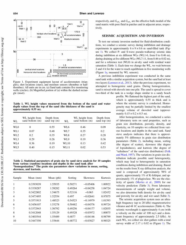
To test our seismic inversion method for fluid-distribution condi-tions, we conduct a seismic survey during imbibition and drainageexperiments in approximately 6 × 9 × 0.6 m sand-filled tank (Fig-ure 1). We collect P- and S-wave pseudo-walkaway seismic dataduring imbibition at six different WLs (WL1-6, from 0 to 0.46 m),during draining at five different WLs (WL7-11, from 0.46 to 0.02 m),and for a reference test (WL0) in air-dry sand with residual watersaturation (Table 1). Each time we change the WL, we wait between2 and 4 h for the water to reach equilibrium in five monitoring wells(Figure 1a, measured by WL sensors).A previous imbibition experiment was conducted in the same
sand tank with a similar acquisition system, but the sand had at leasttwo layers (Lorenzo et al., 2013). After the previous experiment, weattempted to homogenize sand grains. During homogenization,sand is mixed with shovels into one pile. The sand is spread to covertwo-third of the tank in a wedge shape similar to a sandy beach
profile. We flattened the highest part of the sand,which is approximately 0.55 m thick and iswhere the seismic survey is conducted. Homo-geneity may be partially limited by the smallestaverage volume of shoveled sand (approxi-mately 0.15 × 0.2 × 0.5 m).After homogenization, we conducted a series
of laboratory tests on sand properties, such asgrain size distribution, porosity, density, andelasticity, on 10 samples we collected from vari-ous locations and depths in the sand tank. Sandsieve analysis indicates that there is approxi-mately 5% difference in grain size distributionparameters (Table 2), including mean, sorting(the degree of scatter), skewness (the degreeof lopsidedness), and kurtosis (the degree of“tailedness” of the sand-size distribution) (Folkand Ward, 1957). The variations in grain size dis-tribution indicate possible sand heterogeneity,which may lead to heterogeneity in saturationconditions during imbibition and draining. Basedon the results from X-ray diffraction analysis, thesand is composed of approximately 98% ofquartz, approximately 1% of K-feldspar, and ap-proximately 1% of plagioclase. We use the elas-ticity of quartz (Mavko et al., 2009) for ourvelocity prediction (Table 3). From laboratorymeasurements of sample weight and volume,we also determine bulk density for air-dry sandand porosity for air-dry and wet sand (Table 3).The seismic acquisition system uses an ultra-
high frequency (up to 20 kHz) magnetostrictivevibrator and 48 1C accelerometers (Table 4). Theseismic wavelength is approximately 4 cm (witha velocity on the order of 100 m∕s and a dom-inant frequency of approximately 2.5 kHz). Ateach WL, we collect six shot gathers with a totalsurvey width of 2.17� 0.02 m (Figure 1). The
Table 1. WL height values measured from the bottom of the sand and waterdepth values from the top of the sand (the thickness of the sand isapproximately 0.55 m).
WLWL height fromsand bottom (m)
Depth fromsand top (m) WL
WL height fromsand bottom (m)
Depth fromsand top (m)
WL0 0 0.55 WL6 0.46 0.09
WL1 0.07 0.48 WL7 0.35 0.2
WL2 0.2 0.35 WL8 0.27 0.28
WL3 0.29 0.26 WL9 0.19 0.36
WL4 0.36 0.19 WL10 0.13 0.42
WL5 0.40 0.15 WL11 0.02 0.53
Figure 1. Experiment equipment layout of accelerometers (trian-gles), shot locations (stars), and moisture sensors (rhombus or half-rhombus). All units are in cm. (a) Sand tank contains five monitoringwells (circles). (b) Magnified portion of (a) within the dashed rectan-gle (inset).
Table 2. Statistical parameters of grain size by sand sieve analysis for 10 samplesfrom various (random) locations and depths in the sand tank after“homogenization.” The grain size parameters show variations in mean, sorting,skewness, and kurtosis.
Sample Mean (mm) Mean (phi) Sorting Skewness Kurtosis
1 0.3393039 1.55935 0.50271 −0.05406 1.00922
2 0.3338287 1.58282 0.49264 −0.04258 1.04724
3 0.3422802 1.54675 0.52116 −0.063 1.02432
4 0.3473495 1.52554 0.497 −0.02641 0.97075
5 0.3571915 1.48523 0.54523 −0.14979 1.01593
6 0.3456107 1.53278 0.50482 −0.04576 0.99724
7 0.3372943 1.56792 0.49256 −0.04177 1.02035
8 0.3412048 1.55129 0.49328 −0.03972 1.00075
9 0.3403544 1.55489 0.4877 −0.04146 0.98799
10 0.3447350 1.53644 0.48772 −0.03827 0.98525
U54 Shen and Lorenzo
Dow
nloa
ded
08/1
6/16
to 1
30.3
9.18
8.13
7. R
edis
trib
utio
n su
bjec
t to
SEG
lice
nse
or c
opyr
ight
; see
Ter
ms
of U
se a
t http
://lib
rary
.seg
.org
/
vibration source is oriented vertically and horizontally. In total, 24accelerometers are buried (3 cm depth) in one row and oriented withthe most sensitive axis parallel to source vibration direction. An-other 24 accelerometers are buried (also at 3 cm) in another rowand oriented with the most sensitive axis orthogonally to the source,hence they can capture SH-waves (Figure 1b). The accelerometersare placed 1.5 cm apart (center to center) for a total array length of34.5� 0.2 cm. There are a total of six shots for each pseudo-walk-away survey. The first shot offset is 3 cm (center to center), and eachsubsequent shot location is moved 36 cm (Figure 1b).To determine VP and VS-versus-depth profiles, we attempt to best
match the traveltimes of refracted and reflected first arrivals of P-and S-waves by forward-tracing rays (Cerveny, 2001) with 1D gra-dient-velocity layers (shown with P-wave examples in Figure 2).The thickness of each velocity layers can also be determined withforward ray-tracing modeling. For postcritically refracted rays,velocity values over any given depth range are associated withmaterial properties that lie halfway, horizontally, between sourceand receiver. Averaging may occur, but only within each given con-stant- or constant-gradient-velocity depth interval.During processing, seismic amplitudes are rebalanced through
division by the root-mean-square (rms) average at each recorded ac-celerometer with a window width of 0.002 s. Band-pass frequencyfiltering between 200 and 5000 Hz is applied to suppress noise. InFigure 2, the straight or slightly concave-upward seismic events cor-respond to P-wave refractions within the sand body (higher slope)and from the concrete bottom of the tank (lower slope). The higherslope refraction arrivals can be best matched by two velocity layerswith distinct gradients, whereas the lower slope arrivals can be bestmatched by a constant velocity approximately 2000 m∕s. The con-cave-downward seismic arrival approximately 0.008 s is interpretedto correspond to a P-wave reflection from the bottom of the sand tankand can be best matched by a sharp velocity increase from approx-imately 150 to 2000 m∕s. We set the P-wave velocity scale from ap-proximately 110 to 180 m∕s in Figure 2 to show velocity changes insands, hence the velocity layer (approximately 2000 m∕s) for theconcrete bottom of the tank could not be shown. TheVP-versus-depthprofile from WL2 is also representative of WL1-3, and the profilefrom WL 4 is representative for WL0, 4, 5, and 7-11. S-wave refrac-tion arrivals, which have a straight or slightly concave-upward shape,can be best matched by a single layer showing a consistent-velocitygradient. S-wave refraction arrivals have a larger slope than P-wave
refraction but similar to Rayleigh wave refraction arrivals in Figure 2.S-wave reflections that have a concave-downward shape are inter-preted to reflect from the bottom of the sand tank. Compared withVP, VS is less sensitive to changes in water saturation and depth.Velocity profiles represent average velocities within each layer overthe seismic survey width (2.17 m). The error in velocity is less than�2% (from�10−4 s error in traveltime). We extract VP and VS at thedepths of 0.1 and 0.37 m from VP- and VS-versus-depth profiles(Figure 2) to show velocity changes with various WLs and water sat-urations at a given depth (Figure 3). These depths are chosen to re-present the central portion of two zones with distinct velocitygradients (Figure 2).To show changes in seismic velocity with water saturation and
verify inverted saturation results, we also measure volumetric watercontent during experiments with five moisture sensors buried hori-zontally in the sand at different depths (0.1, 0.19, 0.28, 0.37, and0.46 m). These capacitance-/frequency-domain sensors detect thevolumetric water content by measuring the dielectric constant ofthe sand (Table 4). The readings from moisture sensors are collectedfor 90 s (at the rate of 1 sample∕s) each time after the WL reachesequilibrium and before seismic acquisition. We self-calibrate thesensors by determining a linear relationship between the sensor’svoltage readings and volumetric water content measured fromgravimetric sampling methods using oven drying (Dane and Topp,2002; Czarnomski et al., 2005) for air-dry and wet sands in the sandtank. The volumetric water content is calculated with the self-calibrated linear relationship from the average voltage of the
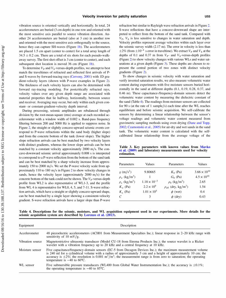
Table 3. Key parameters with known values from Mavkoet al. (2009) and laboratory measurements used for velocityestimation.
Parameters Values Parameters Values
g (m∕s2) 9.80665 K0 (Pa) 3.66 × 10¹⁰
ρw (kg∕m3) 1 G0 (Pa) 4.5 × 10¹⁰
ρa (kg∕m3) 1.18 × 10⁻³ ρ0 (kg∕m3) 2.65
Kw (Pa) 2.2 × 10⁹ ρeff (dry, kg∕m3) 1.54
Ka (Pa) 1.01 × 10⁵ ϕ (wet) 0.4
C 3 ϕ (dry) 0.43
Table 4. Descriptions for the seismic, moisture, and WL acquisition equipment used in our experiments. More details for theseismic acquisition system are described by Lorenzo et al. (2013).
Equipment Description
Accelerometer 48 piezoelectric accelerometers (ACH01 from Measurement Specialties Inc.); linear response in 2–20 kHz range withsensitivity of 10 mV∕g.
Vibration source Magnetostrictive ultrasonic transducer (Model CU-18 from Etrema Products Inc.); the source wavelet is a Rickerwavelet with a vibration frequency up to 20 kHz and a central frequency at 10 kHz.
Moisture sensor Five capacitance/frequency-domain sensors (EC-5 from Decagon Devices Inc.); the maximum measurement volumeis 240 ml for a cylindrical volume with a radius of approximately 3 cm and a height of approximately 10 cm; theaccuracy is �2%; the resolution is 0.001 m3∕m3; the measurement range is from zero to saturation; the operatingtemperature is −40 to 60°C.
WL sensor Five submersible pressure transducers (WL400 from Global Water Instrumentation Inc.); the accuracy is �0.1%;the operating temperature is −40 to 85°C.
Velocity inversion for patchy saturation U55
Dow
nloa
ded
08/1
6/16
to 1
30.3
9.18
8.13
7. R
edis
trib
utio
n su
bjec
t to
SEG
lice
nse
or c
opyr
ight
; see
Ter
ms
of U
se a
t http
://lib
rary
.seg
.org
/
90 s voltage readings. Then, we plot the observed seismic velocityagainst water saturation at depths of 0.1 and 0.37 m (Figure 4).To determine fluid-distribution conditions, we use rock-physics
models with different fluid distribution assumptions to best matchexperimental VP and VS-versus-depth profiles (Figure 5). We beginour inversion by inputting elasticity values for quartz sand (Mavkoet al., 2009) and values for porosity and bulk density of air-driedsand, derived from samples in the sand tank. These known propertyvalues help to constrain inverted results and accelerate the inversion(Table 3). The inversion results include SWCC, Sw, and the volu-metric fraction of the patches (Figure 5). We minimize the misfitbetween experimental and predicted VP and VS-versus-depth
profiles for each WL, aided by the covariance matrix adaptationevolution strategy optimization (Shen et al., 2015). The best fit forthe experimental data relies on the lowest rms misfit to arrive at thepreferable inversion result. Like the effective bulk modulus, the ef-fective shear modulus is averaged according to equations 12 and 15as well. As VP is more sensitive to water saturation changes than VS,inverted SWCC and saturation results depend on mostly on VP-versus-depth profiles. Velocity prediction models are based on theHM-BG model, but have three different averaging methods depend-ing on their respective fluid distribution assumptions: (1) HM-BGfor homogeneous saturation (average using equation 13), (2) HM-BG-Wood for small-sized patchy saturation (average using equa-
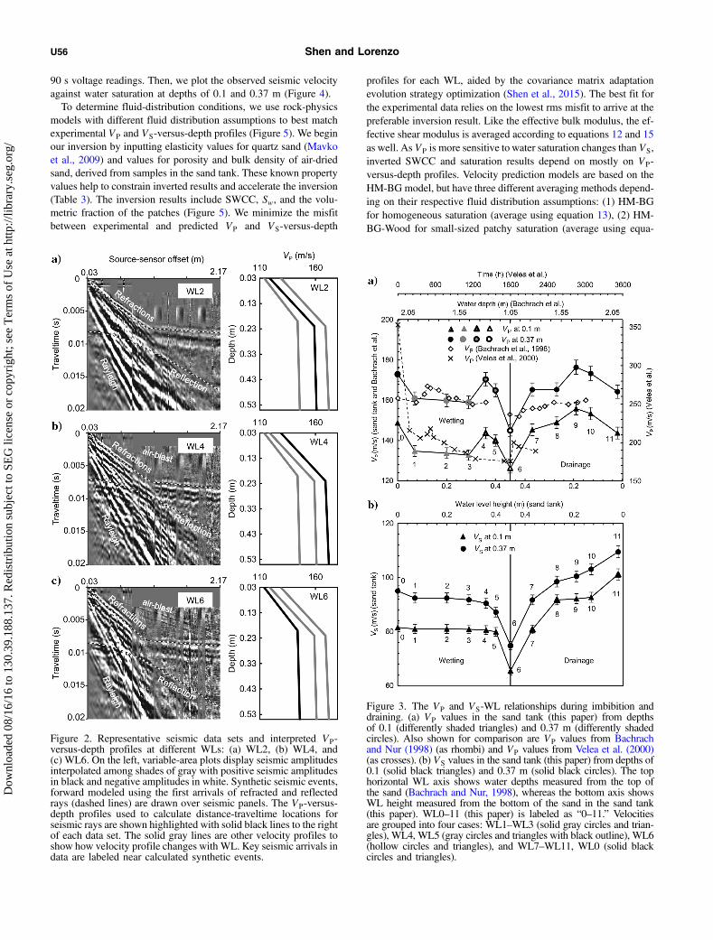
Figure 2. Representative seismic data sets and interpreted VP-versus-depth profiles at different WLs: (a) WL2, (b) WL4, and(c) WL6. On the left, variable-area plots display seismic amplitudesinterpolated among shades of gray with positive seismic amplitudesin black and negative amplitudes in white. Synthetic seismic events,forward modeled using the first arrivals of refracted and reflectedrays (dashed lines) are drawn over seismic panels. The VP-versus-depth profiles used to calculate distance-traveltime locations forseismic rays are shown highlighted with solid black lines to the rightof each data set. The solid gray lines are other velocity profiles toshow how velocity profile changes with WL. Key seismic arrivals indata are labeled near calculated synthetic events.
Figure 3. The VP and VS-WL relationships during imbibition anddraining. (a) VP values in the sand tank (this paper) from depthsof 0.1 (differently shaded triangles) and 0.37 m (differently shadedcircles). Also shown for comparison are VP values from Bachrachand Nur (1998) (as rhombi) and VP values from Velea et al. (2000)(as crosses). (b) VS values in the sand tank (this paper) from depths of0.1 (solid black triangles) and 0.37 m (solid black circles). The tophorizontal WL axis shows water depths measured from the top ofthe sand (Bachrach and Nur, 1998), whereas the bottom axis showsWL height measured from the bottom of the sand in the sand tank(this paper). WL0–11 (this paper) is labeled as “0–11.” Velocitiesare grouped into four cases: WL1–WL3 (solid gray circles and trian-gles), WL4, WL5 (gray circles and triangles with black outline), WL6(hollow circles and triangles), and WL7–WL11, WL0 (solid blackcircles and triangles).
U56 Shen and Lorenzo
Dow
nloa
ded
08/1
6/16
to 1
30.3
9.18
8.13
7. R
edis
trib
utio
n su
bjec
t to
SEG
lice
nse
or c
opyr
ight
; see
Ter
ms
of U
se a
t http
://lib
rary
.seg
.org
/
tion 12), and (3) HM-BG-Hill for large-sized patchy saturation(average using equation 15).
RESULTS
The VP-WL (Figures 3a) and VP-Sw (Figures 4) relationships arenonmonotonic in the shallow (represented by the depth at 0.1 m)and deep (represented by the depth at 0.37 m) sand. No generaltrend can be observed throughout the imbibition or drainage. Dur-ing imbibition, VP values oscillate from peak to trough twice. Thepeaks of the VP value occur in air-dry sand (WL0) and WL4. VP
reaches the lowest value at the highest WL and water saturation(WL6). During drainage, the VP-WL relationship has a transitionbetween increasing and decreasing trends, and the peak of theVP value occurs at WL9 (Figure 3a).In contrast to the nonmonotonic VP-WL relationship, the VS-WL
relationship is monotonic during the imbibition and drainage of thesand (Figure 3b). VS values decrease throughout the imbibition(WL1-6) and increase throughout the drainage (WL7-11).Based on the inversion results and the VP-versus-depth profiles
among 12 WLs (WL0–WL11), we distinguish four representative
cases for four different groups to summarize the results (Figure 3).VP-versus-depth profiles and inversion results differ by less than�3% within each case and larger than 7% in different cases.(Case 1) During the earliest stage of imbibition (WL1-3, repre-
sented by WL2), velocity-versus-depth profiles are best fit by theHM-BG-Wood model (Figure 6a). (Case 2) During the middle stageof imbibition (WL4 and WL5, represented by WL4), velocity-ver-sus-depth profiles are best fit by the HM-BG-Hill model (Figure 6b).(Case 3) When WL is the highest (WL6), velocity-versus-depthprofiles are best fit by the HM-BG-Wood and the HM-BG models(Figure 6c). (Case 4) During draining (WL7-11, WL0, representedby WL10), velocity-versus-depth profiles are best fit by the HM-BG-Hill model (Figure 6d).The quality for the inversion results can be shown by the good
correlation between inverted water saturation with measured in situwater saturation. Average measured water saturation for each VP
value in the sand tank is calculated using arithmetic average of thewater saturation at each depth. The inverted water saturation agreeswith the measured water saturation with a difference of less than 7%for all WLs (Figure 7). The error is �2% in measured water satu-ration (from instrument error). The inverted water saturation has anerror of �10%, which is determined using a Monte Carlo methodafter 100 inversion attempts (Shen et al., 2015). The difference be-tween inverted and measured water saturation is within the error ofthe inverted water saturation.
DISCUSSION
Although our experiment is conducted once, similar observed non-monotonic VP-WL relationships have been described in a laboratorytest with Ottawa Sand (Velea et al., 2000) and tidal experiments at asandy beach (Bachrach and Nur, 1998) (Figure 3a). Consistent withthe observations made by Bachrach and Nur (1998) and Velea et al.(2000), there are two oscillations inVP values during imbibitions, andthe VP value is the lowest at the highest WL. During drainage, thetransition from an increasing to a decreasing trend in our VP-WLrelationship is in agreement with the observation made by Velea et al.(2000) (Figure 3a). However, Bachrach and Nur (1998) only observean increasing trend during the drainage (Figure 3a). The different ob-servations are attributed to the differences in sediment heterogeneityand experiment setup (e.g., seismic frequency, injection rate, and thedensity and viscosity of pore fluids) (Homsy, 1987). One possible
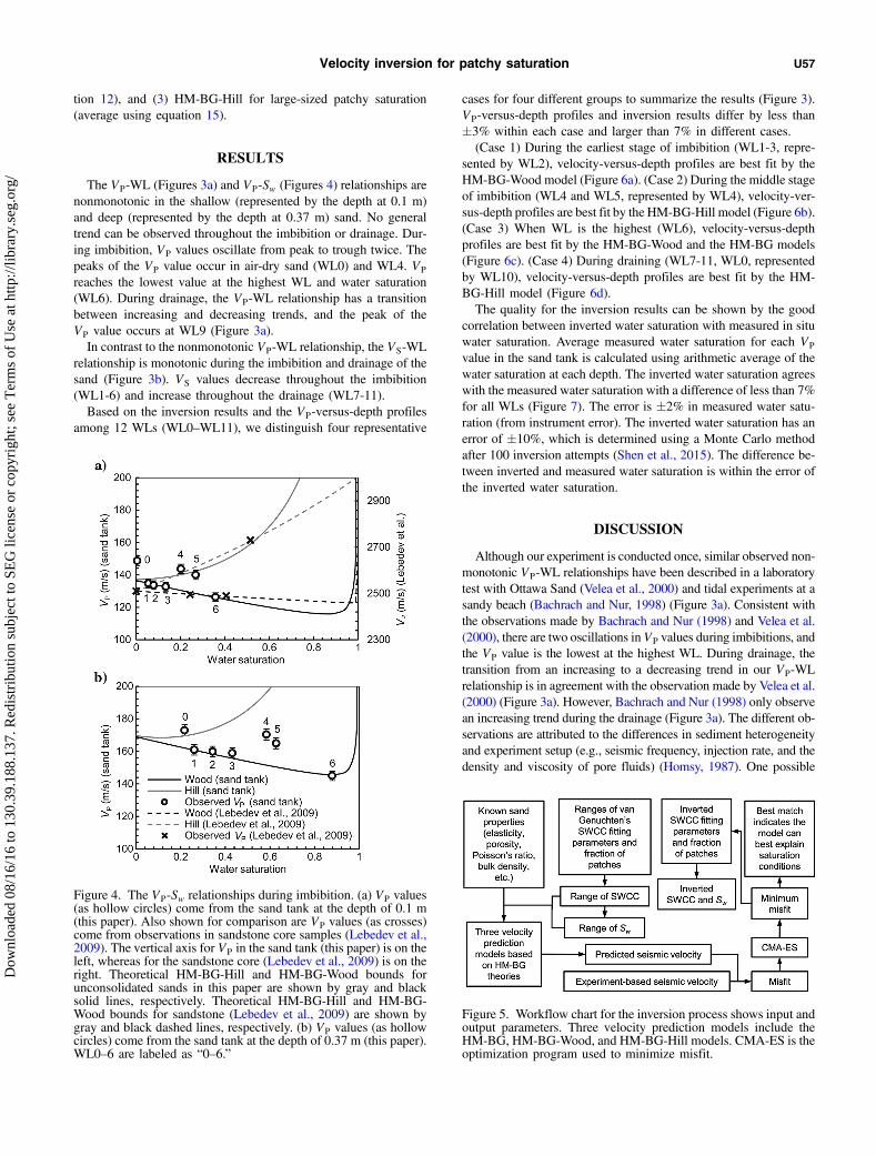
Figure 4. The VP-Sw relationships during imbibition. (a) VP values(as hollow circles) come from the sand tank at the depth of 0.1 m(this paper). Also shown for comparison are VP values (as crosses)come from observations in sandstone core samples (Lebedev et al.,2009). The vertical axis for VP in the sand tank (this paper) is on theleft, whereas for the sandstone core (Lebedev et al., 2009) is on theright. Theoretical HM-BG-Hill and HM-BG-Wood bounds forunconsolidated sands in this paper are shown by gray and blacksolid lines, respectively. Theoretical HM-BG-Hill and HM-BG-Wood bounds for sandstone (Lebedev et al., 2009) are shown bygray and black dashed lines, respectively. (b) VP values (as hollowcircles) come from the sand tank at the depth of 0.37 m (this paper).WL0–6 are labeled as “0–6.”
Figure 5. Workflow chart for the inversion process shows input andoutput parameters. Three velocity prediction models include theHM-BG, HM-BG-Wood, and HM-BG-Hill models. CMA-ES is theoptimization program used to minimize misfit.
Velocity inversion for patchy saturation U57
Dow
nloa
ded
08/1
6/16
to 1
30.3
9.18
8.13
7. R
edis
trib
utio
n su
bjec
t to
SEG
lice
nse
or c
opyr
ight
; see
Ter
ms
of U
se a
t http
://lib
rary
.seg
.org
/
explanation for the difference is that the time durations of the twodrainage processes are different: the drainage in our experiment lastsfor approximately 15 h, whereas in Bachrach and Nur (1998)’s, itlasts approximately 2 h. As a result, their experiment may not havecaptured the decreasing trend in VP-WL relationship during thedrainage.The nonmonotonic VP-Sw relationship can be explained by the
transitions between the HM-BG-Wood and the HM-BG-Hill bounds,depending on the change in patch size (Lebedev et al., 2009) andseismic frequency (Cadoret et al., 1995). We interpret that the tran-
sitions in VP-Sw relationships between the HM-BG-Wood and theHM-BG-Hill bounds are attributed to the variation in the patch sizerelative to the diffusion length (Figures 4 and 6). At low water sat-uration (WL1-3), the VP-Sw relationship follows the HM-BG-Woodbound (Figures 4 and 6a). We interpret that the patches are smallsized (<1 cm) at the beginning of imbibition.When the inverted aver-age water saturation (arithmetic mean) is more than approximately45% (WL4, Figure 7b), VP values have a transition from the HM-BG-Wood to HM-BG-Hill bound (Figures 4a and 6b) or between thetwo bounds (Figures 4b and 6b). We interpret that the large-sizedpatches (>1 cm) start to form during the middle stage of imbibition.WhenWL is the highest (WL6), VP values have a transition from theHM-BG-Hill back to the HM-BG-Wood bound (Figures 4 and 6c).We interpret that the water distribution is relatively homogeneouswith small-sized residual-air patches at the highestWL. During drain-age, the VP-Sw relationship follows the HM-BG-Hill behavior (Fig-ure 6d), and this result is in agreement with previous laboratoryobservations (Murphy, 1982; Knight and Nolen-Hoeksema, 1990;Cadoret et al., 1995; Monsen and Johnstad, 2005;). We interpret thatthe patches are large sized (>1 cm) during drainage.The transition from HM-BG-Wood behavior to HM-BG-Hill
behavior (WL1–WL5) is consistent with a previous laboratory study,which shows that the transition happens when small patches clusteras water saturation exceeds 40% (Figure 4) (Lebedev et al., 2009).During injection of water into a sandstone sample, Lebedev et al.
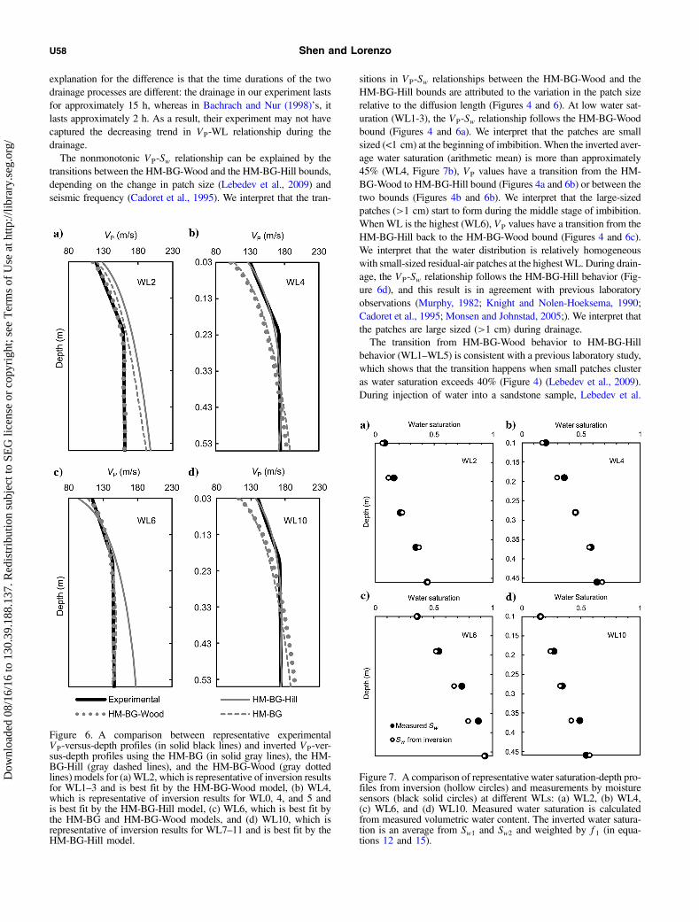
Figure 6. A comparison between representative experimentalVP-versus-depth profiles (in solid black lines) and inverted VP-ver-sus-depth profiles using the HM-BG (in solid gray lines), the HM-BG-Hill (gray dashed lines), and the HM-BG-Wood (gray dottedlines) models for (a) WL2, which is representative of inversion resultsfor WL1–3 and is best fit by the HM-BG-Wood model, (b) WL4,which is representative of inversion results for WL0, 4, and 5 andis best fit by the HM-BG-Hill model, (c) WL6, which is best fit bythe HM-BG and HM-BG-Wood models, and (d) WL10, which isrepresentative of inversion results for WL7–11 and is best fit by theHM-BG-Hill model.
Figure 7. A comparison of representative water saturation-depth pro-files from inversion (hollow circles) and measurements by moisturesensors (black solid circles) at different WLs: (a) WL2, (b) WL4,(c) WL6, and (d) WL10. Measured water saturation is calculatedfrom measured volumetric water content. The inverted water satura-tion is an average from Sw1 and Sw2 and weighted by f1 (in equa-tions 12 and 15).
U58 Shen and Lorenzo
Dow
nloa
ded
08/1
6/16
to 1
30.3
9.18
8.13
7. R
edis
trib
utio
n su
bjec
t to
SEG
lice
nse
or c
opyr
ight
; see
Ter
ms
of U
se a
t http
://lib
rary
.seg
.org
/
(2009) observe that VP decreases slightly and follows the HM-BG-Wood bound at low water saturations.When water saturation exceedsapproximately 40%, VP sharply increases and can be interpreted by atransition from the HM-BG-Wood to HM-BG-Hill bound. Their re-sults from X-ray computer tomography show that the interpretedtransition from the HM-BG-Wood to HM-BG-Hill bound corre-sponds to the clustering of small fluid patches and the formation oflarger patches. Some observations show that the experimental VP-Swrelationship can be explained by the lower velocity bound from theHM-BG-Wood model during imbibition, and the upper velocitybound from the HM-BG-Hill model during drainage (Murphy, 1982;Knight and Nolen-Hoeksema, 1990; Cadoret et al., 1995; Monsenand Johnstad, 2005).The assumptions behind each rock-physics model can be used to
interpret the fluid-distribution condition at WLs. When the HM-BG-Wood model best describes the velocity-versus-depth profiles(WL1-3; Figures 4 and 6a), it suggests that the patch sizes are smallin comparison with the diffusion length (approximately 1 cm in ourunconsolidated sands) at the beginning of the imbibition. However,when the HM-BG-Hill model provides a better fit to the velocity-versus-depth profile, we can interpret that the size of the patchesis larger than the diffusion length (>1 cm) (WL0, 4, 5, 7–11; Fig-ures 4, 6b, and 6d). In the air-dry sand (WL0), the matric suctioncontribution weighted by water saturation (equation 9) is minimumand so the effective pressure is highest. The high effective pressuremay also lead to the relatively high VP value. At WL6 (highest), thebest fit by HM-BG and HM-BG-Wood models indicates that the sat-uration condition is homogeneous (Figures 4 and 6b). For WL6, theinversion results from HM-BG-Wood show that no patches exist.Based on the interpretation of the patch size during the imbibition
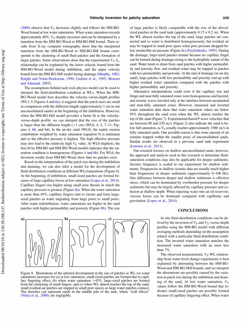
and draining, we can also infer a model for the development offluid-distribution conditions at different WLs/saturations (Figure 8).At the beginning of imbibition, small-sized patches are formed be-cause of large capillary forces at low saturation (Lopes et al., 2014).Capillary fingers rise higher along small pore throats in which thecapillary pressure is greatest (Figure 8a). When the water saturationis more than 45%, capillary fingers start to cluster and form large-sized patches as water migrating from large pores to small pores.After water redistribution, water saturations are higher in the sandpatches with higher permeability and porosity (Figure 8b). The size
of large patches is likely comparable with the size of the shovel-sized patches in the sand tank (approximately 0.15 × 0.2 m). Whenthe WL almost reaches the top of the sand, large patches are con-nected and so water is distributed homogeneously, but residual airmay be trapped in small pore space when pore pressure dropped be-low irreducible air pressure (Figure 8c) (Faybishenko, 1995). Duringthe drainage, large-sized patches remain because no capillary fingercan be formed during drainage owing to the hydrophilic nature of thesand. Water tends to drain from sand patches with higher permeabil-ity and porosity first, and residual water may be trapped in patcheswith less permeability and porosity. At the end of drainage (in air-drysand), large patches with less permeability and porosity end up withhigher residual water saturation compared with the patches withhigher permeability and porosity.Alternative interpretations could exist if the capillary rise and
fringe and near-fully saturated zones were homogeneous and layered,and seismic waves traveled only at the interface between unsaturatedand near-fully saturated zones. However, measured and invertedwater saturation data show that water saturation values are below95% throughout the sand even when the WL almost reaches thetop of the sand (Figure 7). Experimental-based P-wave velocities thatare between 80 and 230 m∕s (Figure 2) also indicate the sand is be-low full saturation, as VP usually reaches approximately 1500 m∕s infully saturated sands. One possible reason is that some amount of airremains trapped within the smaller pores of unconsolidated sands.Similar results are observed in a previous sand tank experiment(Lorenzo et al., 2013).Our research focuses on shallow unconsolidated sands, however,
the approach and analysis used in this research to determine fluid-saturation conditions may also be applicable for deeper sediments.Seismic frequency is scaled in our experiment for shallow sedi-ments. Frequencies in shallow seismic data are usually much higherthan frequencies in deeper sediments (approximately 0–100 Hz).One difference between deeper and shallow sediments is effectivestress, which can be dominated by overburden pressure for deepersediments but may be largely affected by capillary pressure and co-hesion at shallow depth. When injecting water into an oil reservoir,viscous forces can be dominant compared with capillarity andgravitation (Lopes et al., 2014).
CONCLUSIONS
In situ fluid-distribution conditions can be de-rived by the inversion of VP and VS-versus-depthprofiles using the HM-BG model with differentaveraging methods depending on the assumptionrelated with a particular fluid-distribution condi-tion. The inverted water saturation matches themeasured water saturation with an error lessthan 7%.The observed nonmonotonic VP-WL relation-
ship from water-level change experiments is bestexplained by alternating between the HM-BG-Wood and HM-BG-Hill bounds, and we interpretthe alternations are possibly caused by the varia-tion in patch size during the imbibition and drain-ing of the sand. At low water saturation, VP
values follow the HM-BG-Wood bound that in-dicates small-sized patches are possibly formedbecause of capillary fingering effect. When water
Figure 8. Illustrations of the inferred development in the size of patches as WL (or watersaturation) increases for (a) at low saturation, small-sized patches are formed due to capil-lary fingering effect, (b) when water saturation >45%, large-sized patches are formedfrom the clustering of small fingers, and (c) when WL almost reaches the top of the sand,small residual-air patches are trapped in small pore spaces as large water patches connect.The sketches can represent sands in the middle part of the tank, where “wall effects”(Velea et al., 2000) are negligible.
Velocity inversion for patchy saturation U59
Dow
nloa
ded
08/1
6/16
to 1
30.3
9.18
8.13
7. R
edis
trib
utio
n su
bjec
t to
SEG
lice
nse
or c
opyr
ight
; see
Ter
ms
of U
se a
t http
://lib
rary
.seg
.org
/
saturation is more than 45%, VP-Sw relationship shows a transitionfrom the HM-BG-Wood to the HM-BG-Hill bound, and we inter-pret the transition as caused by a change in patch size from smallto large. When WL almost reaches the top of the sand, the VP-Swrelationship shows a transition from the HM-BG-Hill back to theHM-BG-Wood bound, and we interpret this transition as caused bya change from large water-saturated patches to small-sized residual-air patches. During drainage, VP values follow the HM-BG-Hillbound that indicates the patches are large sized because no capillaryfinger can be formed due to the hydrophilic nature of the sand.
ACKNOWLEDGMENTS
This work is supported by a Shell Exploration & ProductionCompany Grant (2011–2015). We would like to thank F. Tsai andH. Pham for their help with optimization techniques, L. Butler andA. Brooks for their help with Labview programming, Ario Labs inBaton Rouge for their help with building the seismic acquisitionsystem, C. Gama for her help with grain size analysis, and R. Youngand C. Li for the support with facilities and the sand tank. We thankthe following for their support with scholarships to the first author:Geometrics Inc. Student Travel Grant for SAGEEP, the DonaldTowse Memorial Fund awarded by AAPG Grant-in-Aid, H. V. An-derson Scholarship, EnCana Scholarship and Imagine ResourcesScholarship awarded by the LSU Department of Geology and Geo-physics, and especially to the LSU Department of Geology and Geo-physics for their active support of graduate student research.
REFERENCES
Bachrach, R., and A. Nur, 1998, High-resolution shallow-seismic experi-ments in sand, Part I: Water table, fluid flow, and saturation: Geophysics,63, 1225–1233, doi: 10.1190/1.1444423.
Biot, M. A., 1962, Mechanics of deformation and acoustic propagation inporous media: Journal of Applied Physics, 33, 1482–1498, doi: 10.1063/1.1728759.
Cadoret, T., D. Marion, and B. Zinszner, 1995, Influence of frequency andfluid distribution on elastic wave velocities in partially saturated lime-stones: Journal of Geophysical Research: Solid Earth, 100, 9789–9803, doi: 10.1029/95JB00757.
Cadoret, T., G. Mavko, and B. Zinszner, 1998, Fluid distribution effect onsonic attenuation in partially saturated limestones: Geophysics, 63, 154–160, doi: 10.1190/1.1444308.
Cerveny, V., 2001, Seismic ray theory: Cambridge University Press.Czarnomski, N. M., G. W. Moore, T. G. Pypker, J. Licata, and B. J. Bond,
2005, Precision and accuracy of three alternative instruments for meas-uring soil water content in two forest soils of the Pacific Northwest: Cana-dian Journal of Forest Research, 35, 1867–1876, doi: 10.1139/x05-121.
Dane, J. H., and G. C. Topp, 2002, Methods of soil analysis: Part 4. Physicalmethods: Soil Society of America.
DiCarlo, D. A., 2003, Drainage in finite-sized unsaturated zones: Advances inWater Resources, 26, 1257–1266, doi: 10.1016/j.advwatres.2003.09.001.
Dvorkin, J., and A. Nur, 1998, Acoustic signatures of patchy saturation:International Journal of Solids and Structures, 35, 4803–4810, doi: 10.1016/S0020-7683(98)00095-X.
Faybishenko, B. A., 1995, Hydraulic behavior of quasi‐saturated soils in thepresence of entrapped air: Laboratory experiments: Water ResourcesResearch, 31, 2421–2435, doi: 10.1029/95WR01654.
Folk, R. L., and W. C. Ward, 1957, Brazos River bar: A study in the sig-nificance of grain size parameters: Journal of Sedimentary Research, 27,3–26.
Gassmann, F., 1951, Elastic waves through a packing of spheres: Geophys-ics, 16, 673–685, doi: 10.1190/1.1437718.
Hertz, H., 1882, On the contact of rigid elastic solids and on hardness, chap-ter 6: Assorted papers by H. Hertz: MacMillan.
Hill, R., 1963, Elastic properties of reinforced solids: Some theoretical prin-ciples: Journal of the Mechanics and Physics of Solids, 11, 357–372.
Homsy, G. M., 1987, Viscous fingering in porous media: Annual Review ofFluid Mechanics, 19, 271–311, doi: 10.1146/annurev.fl.19.010187.001415.
Knight, R., J. Dvorkin, and A. Nur, 1998, Acoustic signatures of partial sat-uration: Geophysics, 63, 132–138, doi: 10.1190/1.1444305.
Knight, R., and R. Nolen-Hoeksema, 1990, A laboratory study of the depend-ence of elastic wave velocities on pore scale fluid distribution: GeophysicalResearch Letters, 17, 1529–1532, doi: 10.1029/GL017i010p01529.
Lebedev, M., J. Toms-Stewart, B. Clennell, M. Pervukhina, V. Shulakova, L.Paterson, T. M. Müller, B. Gurevich, and F. Wenzlau, 2009, Direct labo-ratory observation of patchy saturation and its effects on ultrasonic veloc-ities: The Leading Edge, 28, 24–27, doi: 10.1190/1.3064142.
Lopes, S., M. Lebedev, T. M. Müller, M. B. Clennell, and B. Gurevich, 2014,Forced imbibition into a limestone: Measuring P‐wave velocity and watersaturation dependence on injection rate: Geophysical Prospecting, 62,1126–1142, doi: 10.1111/1365-2478.12111.
Lorenzo, J. M., D. E. Smolkin, C. White, S. R. Chollett, and T. Sun, 2013,Benchmark hydrogeophysical data from a physical seismic model: Com-puters & Geosciences, 50, 44–51, doi: 10.1016/j.cageo.2012.07.034.
Løvoll, G., Y. Méheust, K. J. Måløy, E. Aker, and J. Schmittbuhl, 2005,Competition of gravity, capillary and viscous forces during drainage ina two-dimensional porous medium, a pore scale study: Energy, 30,861–872, doi: 10.1016/j.energy.2004.03.100.
Lu, N., and W. J. Likos, 2006, Suction stress characteristic curve for unsatu-rated soil: Journal of Geotechnical and Geoenvironmental Engineering,132, 131–142, doi: 10.1061/(ASCE)1090-0241(2006)132:2(131.
Mavko, G., T. Mukerji, and J. Dvorkin, 2009, The rock physics handbook:Tools for seismic analysis of porous media: Cambridge University Press.
Mindlin, R. D., 1949, Compliance of elastic bodies in contact: Journal ofApplied Mechanics, 16, 259–268.
Monsen, K., and S. Johnstad, 2005, Improved understanding of velocity–saturation relationships using 4D computer‐tomography acoustic measure-ments: Geophysical Prospecting, 53, 173–181, doi: 10.1111/j.1365-2478.2004.00464.x.
Müller, T. M., B. Gurevich, and M. Lebedev, 2010, Seismic wave attenuationand dispersion resulting from wave-induced flow in porous rocks — A re-view: Geophysics, 75, no. 5, 75A147–175A164, doi: 10.1190/1.3463417.
Murphy, W. F., 1982, Effects of partial water saturation on attenuation inMassilon sandstone and Vycor porous glass: The Journal of the Acous-tical Society of America, 71, 1458–1468, doi: 10.1121/1.387843.
Norris, A. N., 1993, Low-frequency dispersion and attenuation in partiallysaturated rocks: The Journal of the Acoustical Society of America, 94,359–370, doi: 10.1121/1.407101.
Riaz, A., G.-Q. Tang, H. A. Tchelepi, and A. R. Kovscek, 2007, Forcedimbibition in natural porous media: Comparison between experimentsand continuum models: Physical Review E, 75, 036305, doi: 10.1103/PhysRevE.75.036305.
Shen, J., J. M. Lorenzo, C. D. White, and F. Tsai, 2015, Soil density, elas-ticity, and the soil-water characteristic curve inverted from field-basedseismic P-and S-wave velocity in shallow nearly saturated layered soils:Geophysics, 80, no. 3, WB11–WB19, doi: 10.1190/geo2014-0119.1.
Song, Y.-S., W.-K. Hwang, S.-J. Jung, and T.-H. Kim, 2012, A comparativestudy of suction stress between sand and silt under unsaturated conditions:Engineering Geology, 124, 90–97, doi: 10.1016/j.enggeo.2011.10.006.
Toms-Stewart, J., T. M. Müller, B. Gurevich, and L. Paterson, 2009, Stat-istical characterization of gas-patch distributions in partially saturatedrocks: Geophysics, 74, no. 2, WA51–WA64, doi: 10.1190/1.3073007.
van Genuchten, M. T., 1980, A closed-form equation for predicting the hy-draulic conductivity of unsaturated soils: Soil Science Society of AmericaJournal, 44, 892–898, doi: 10.2136/sssaj1980.03615995004400050002x.
Velea, D., F. D. Shields, and J. M. Sabatier, 2000, Elastic wave velocities inpartially saturated Ottawa sand: Soil Science Society of America Journal,64, 1226–1234, doi: 10.2136/sssaj2000.6441226x.
Wood, A. B., 1941, A textbook of sound: George Bell & Sons.