29
Selected Topics in Data Networking Explore Social Networks: Prestige and Ranking
| Date post: | 29-Dec-2015 |
| Category: |
Documents |
| Upload: | timothy-cain |
| View: | 218 times |
| Download: | 3 times |
Selected Topics in Data Networking
Explore Social Networks: Prestige and Ranking
Introduction
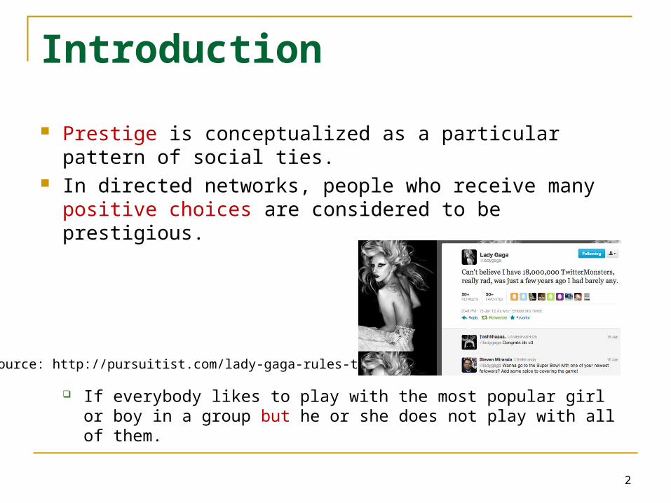
Prestige is conceptualized as a particular pattern of social ties.
In directed networks, people who receive many positive choices are considered to be prestigious.
If everybody likes to play with the most popular girl or boy in a group but he or she does not play with all of them.
2
Source: http://pursuitist.com/lady-gaga-rules-twitter/
Introduction
Popularity and Indegree: Prestige When ties are associated to some positive
aspects such as friendship or collaboration, indegree is often interpreted as a form of popularity, outdegree is interpreted as gregariousness.
A prestigious art museum receives more attention from art critics than less prestigious ones.
3
Source: http://en.wikipedia.org/wiki/Centrality

Introduction
The simplest measure of structural prestige is called popularity and it is measured by the number of choices a vertex receives: its indegree
In undirected networks, we cannot measure prestige; instead, we use degree as a simple measure of centrality.
4

Introduction
We should note that indegree does reflect prestige if we transpose the arcs in such a network, that is, if we reverse the direction of arcs. It is interesting to note that several structural
properties of a network do not change when the arcs are transposed
5

Correlation
Structural prestige scores: Correlation coefficients range from -1 to 1 A positive coefficient indicates that a high score on one feature is
associated with a high score on the other (e.g., high structural prestige occurs in families with high social status).
A negative coefficient points toward a negative or inverse relation: a high score on one characteristic combines with a low score on the other (e.g., high structural prestige is found predominantly with low social status families).
6
Correlation
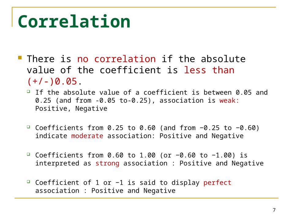
There is no correlation if the absolute value of the coefficient is less than (+/-)0.05. If the absolute value of a coefficient is between 0.05 and 0.25 (and
from -0.05 to-0.25), association is weak: Positive, Negative
Coefficients from 0.25 to 0.60 (and from −0.25 to −0.60) indicate moderate association: Positive and Negative
Coefficients from 0.60 to 1.00 (or −0.60 to −1.00) is interpreted as strong association : Positive and Negative
Coefficient of 1 or −1 is said to display perfect association : Positive and Negative
7
Domains
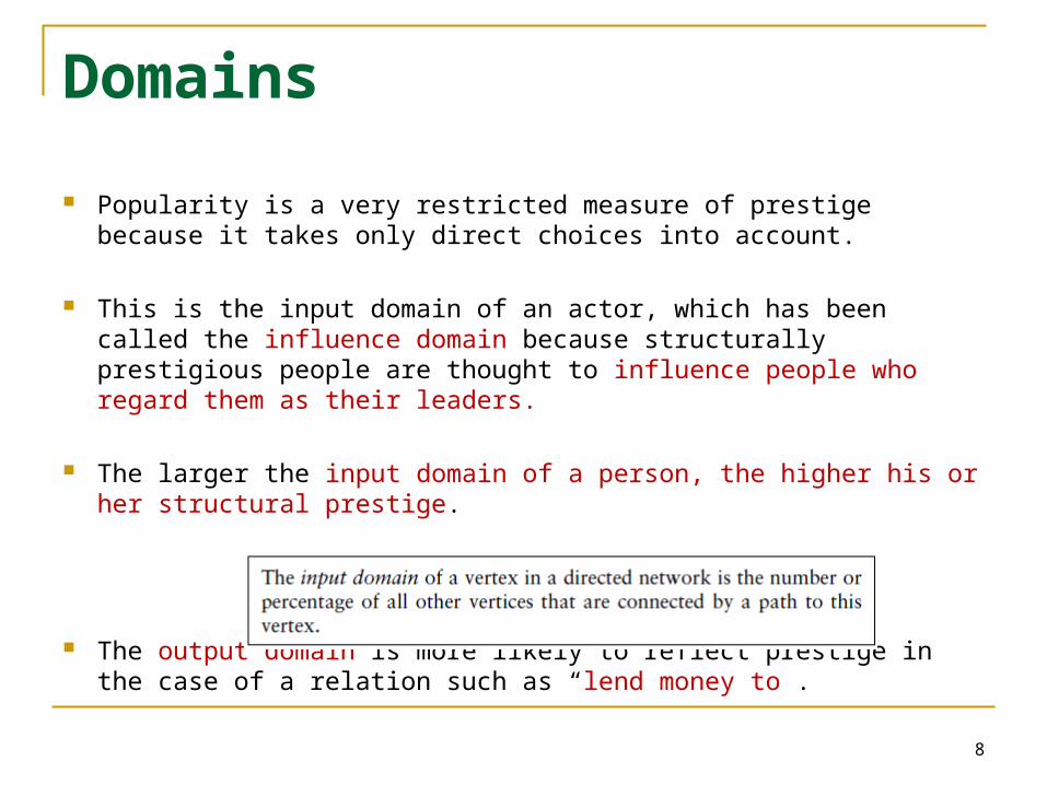
Popularity is a very restricted measure of prestige because it takes only direct choices into account.
This is the input domain of an actor, which has been called the influence domain because structurally prestigious people are thought to influence people who regard them as their leaders.
The larger the input domain of a person, the higher his or her structural prestige.
The output domain is more likely to reflect prestige in the case of a relation such as “lend money to”.
8

Proximity Prestige
Limit the input domain to direct neighbors or to neighbors at maximum distance two on the assumption that nominations by close neighbors are more important than nominations by distant neighbors.
An indirect choice contributes less to prestige if it is mediated by a longer chain of intermediaries.
9

Proximity Prestige
Proximity Prestige: This index of prestige considers all vertices within the input domain of a vertex but it attaches more importance to a nomination if it is expressed by a closer neighbor.
A nomination by a close neighbor contributes more to the proximity prestige of an actor than a nomination by a distant neighbor, but many “distant nominations” may contribute as much as one “close nomination.”
10

Proximity Prestige
To allow direct choices to contribute more to the prestige of a vertex than indirect choices, proximity prestige weights each choice by its path distance to the vertex.
A higher distance yields a lower contribution to the proximity prestige of a vertex, but each choice contributes something.
11
Proximity Prestige
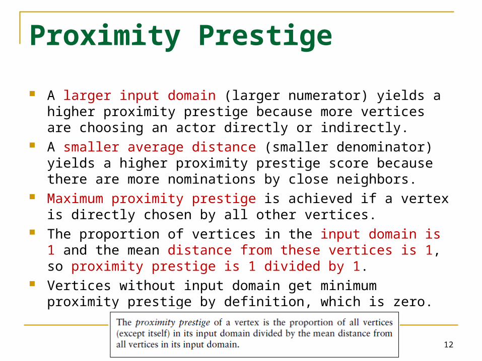
A larger input domain (larger numerator) yields a higher proximity prestige because more vertices are choosing an actor directly or indirectly.
A smaller average distance (smaller denominator) yields a higher proximity prestige score because there are more nominations by close neighbors.
Maximum proximity prestige is achieved if a vertex is directly chosen by all other vertices.
The proportion of vertices in the input domain is 1 and the mean distance from these vertices is 1, so proximity prestige is 1 divided by 1.
Vertices without input domain get minimum proximity prestige by definition, which is zero.
12

Proximity Prestige
All vertices at the extremes of the network (v2, v4, v5, v6,and v10) have empty input domains, hence they have a proximity score of zero.
The input domain of vertex v9 contains vertex v10 only, so its input domain size is 1 out of 9 (.11).
Average distance within the input domain of vertex v9 is one, so the proximity prestige of vertex 9 is .11 divided by 1 = 0.11.
Vertex v1 has a maximal input domain (9 out of 9 =1), Average distance is 2.0, so proximity prestige amounts to 1.00
divided by 2.0, which is .5. Avg.dist. = (4+3+2+1+1+1+2+2+2)/9 = 2
13

Selected Topics in Data Networking
Explore Social Networks: Genealogies and Citations

Introduction
Social communities and intellectual traditions can be defined by a common set of ancestors, by structural relinking (families which intermarry repeatedly), or by long-lasting co-citation of papers. Genealogy Analysis: Pedigree is also important for the
retrospective attribution of prestige to ancestors. Citation analysis: The number of descendants (citations) is used
to assign importance and influence to precursors.
15
Source: https://lonniesmart2k10.wordpress.com/2010/11/23/a-deeper-look-to-your-history-through-genealogy-research/
Source: http://www.mikegrehan.com/?p=22

Genealogy Analysis
Many people are assembling their family trees. Genealogies contain persons as units and two types
of relations among persons: birth and marriage.
A person may belong to two nuclear families: a family in which it is a child and a family in which it is a parent. Child: the family of child or orientation (FAMC) Parent: the family of spouse or procreation (FAMS).
16

Genealogy Analysis
Petrus Gondola’s family contains his wife and eight children and it is identical to the family of orientation of each of his children.
Family codes are translated to arcs between parents and children.
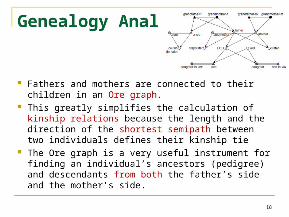
Men are represented by triangles, women by ellipses, marriages by (double) lines, and parent–child ties by arcs. Note that the arcs point from parent to child following the flow of time.
17
Genealogy Analysis
Fathers and mothers are connected to their children in an Ore graph.
This greatly simplifies the calculation of kinship relations because the length and the direction of the shortest semipath between two individuals defines their kinship tie
The Ore graph is a very useful instrument for finding an individual’s ancestors (pedigree) and descendants from both the father’s side and the mother’s side.
18

Genealogy Analysis
Kinship is a fundamental social relation that is extensively studied by anthropologists and historians.
These genealogies, which are usually very large, enable the study of overall patterns of kinship ties which Reflect cultural norms for marriage: who are
allowed to marry?
19
Citation Analysis
Citations make explicit this frame of reference
They are a valuable source of data for the study of scientific development and scientific communities in scientometrics, history, and the sociology of science.
They reveal the impact of articles and their authors on later scientific work and they signal scientific communities or specialties which share knowledge.
20

Citation Analysis
Articles can cite only articles that appeared earlier, so the network is acyclic. Arcs never point back to older articles just as parents cannot be
younger than their children. Out-degree
A citation network contains one relation, whereas genealogical data concern two relations: parenthood and marriage.
Citations are being used to assess the scientific importance of papers, authors, and journals.
Item receiving more citations is deemed more important.
21

Citation Analysis
Citation analysis reveals such cohesive subgroups and it studies their institutional or paradigmatic background. Specialties are cohesive subgroups in the citation network
Weak components identify isolated scientific communities that are not aware of each other or who see no substantial overlap between their research domains
22
Citation Analysis
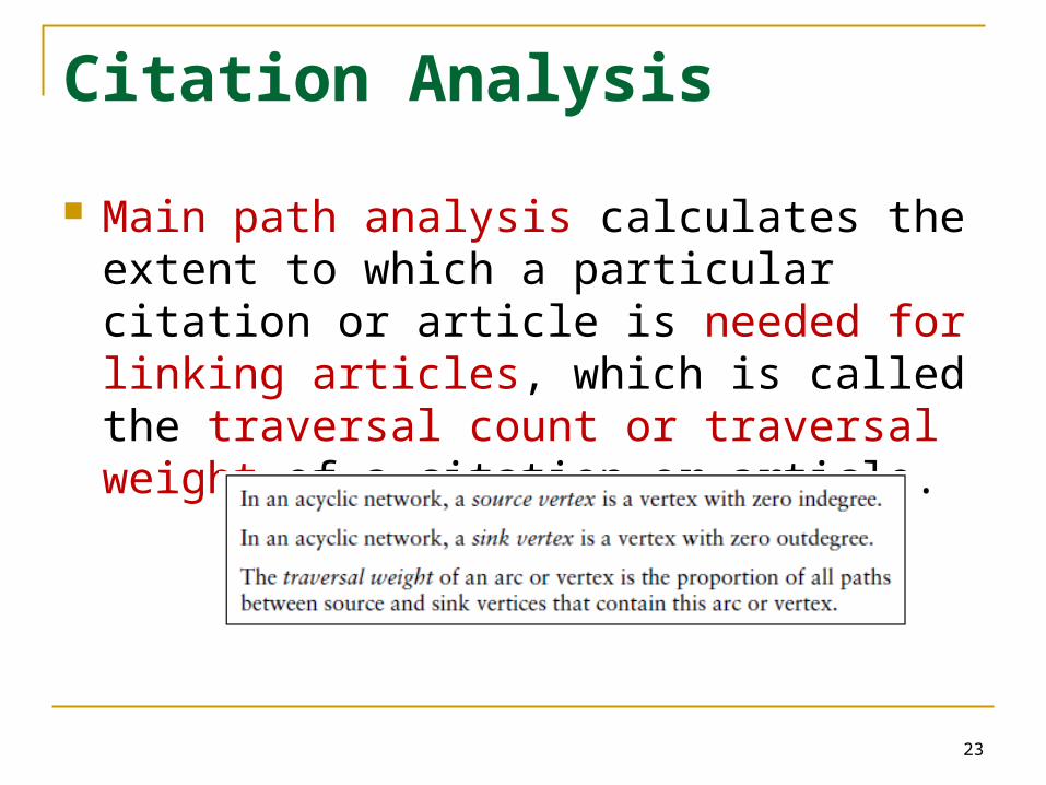
Main path analysis calculates the extent to which a particular citation or article is needed for linking articles, which is called the traversal count or traversal weight of a citation or article.
23

Citation Analysis
There are two sources (v1 and v5) and two sinks (v3 and v4).
There are eight paths from sources to sinks Four paths reach v4 from v1 and three paths from
v5 and one path from v1 to v3
24

Citation Analysis
Traversal Weight (between sources and sinks) Possible paths:
v1:v3, v1=>v3 v1: v4, v1=>v4, v1=>v6=>v2=>v4, v1=>v6=>v4 v5:v3, none v5:v4, v5=>v2=>v4, v5=>v6=>v2=>v4, v5=>v6=>v4
V1: 5/8= 0.625 V5: 3/8= 0.375 V4: 6/8= 0.75 V3: 1/8=0.125
25

Citation Analysis
Main path is the path from a source vertex to a sink vertex with the highest traversal weights on its arcs.
Choosing the source vertex (or vertices) incident with the arc(s) with the highest weight, selecting the arc(s) and the head(s)of the arc(s), and repeating this step until a sink vertex is reached.
26

Citation Analysis
The main paths start with vertex v1 and vertex v5 because both source vertices are incident with an arc carrying a traversal weight of 0.25.
Both arcs point toward vertex v6, which is the next vertex on the main paths.
Then, the paths proceed either to vertex v2 and on to vertex v4 or directly from vertex v6 to vertex v4.
We find several main paths, but they lead to the same sink, so we conclude that the network represents one research tradition.
27
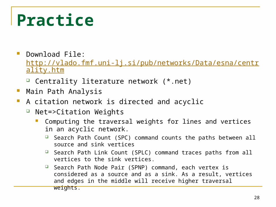
Practice
Download File: http://vlado.fmf.uni-lj.si/pub/networks/Data/esna/centrality.htm Centrality literature network (*.net)
Main Path Analysis A citation network is directed and acyclic
Net=>Citation Weights Computing the traversal weights for lines and vertices in an acyclic
network. Search Path Count (SPC) command counts the paths between all source
and sink vertices Search Path Link Count (SPLC) command traces paths from all vertices to
the sink vertices. Search Path Node Pair (SPNP) command, each vertex is considered as a
source and as a sink. As a result, vertices and edges in the middle will receive higher traversal weights.
28

References
Wouter de Nooy, Andrej Mrvar, and Vladimir Batagelj, Exploratory Social Network Analysis with Pajek, Cambridge
29


