+ All Categories
Home > Documents > Selected Topics in Robust Convex Optimizationnemirovs/PlenaryL_Nemirovski.pdf• In dynamical...

Selected Topics in Robust Convex Optimizationnemirovs/PlenaryL_Nemirovski.pdf• In dynamical...

Date post: 03-Apr-2020
Category:
Upload: others
View: 14 times
Download: 0 times
Share this document with a friend
38
Selected Topics in Robust Convex Optimization Arkadi Nemirovski School of Industrial and Systems Engineering Georgia Institute of Technology Optimization programs with uncertain data and their Robust Counterparts Tractability of Robust Counterparts Robust Optimization and Chance Constraints
Transcript

Selected Topics in Robust ConvexOptimization

Arkadi Nemirovski

School of Industrial and Systems Engineering

Georgia Institute of Technology

• Optimization programs with uncertain data and theirRobust Counterparts

• Tractability of Robust Counterparts• Robust Optimization and Chance Constraints

• Optimization programs with uncertain data and theirRobust Counterparts

• Tractability of Robust Counterparts• Robust Optimization and Chance Constraints

♣ Robust Optimization is a methodology for processing uncer-

tain optimization problems

minx

{f(x, ζ) : F (x, ζ) ∈ K}

• x ∈ Rn is the decision vector

• ζ ∈ Rd is the data (or data perturbation)

• f(x, ζ) : Rn × Rd → R and F (x, ζ) : Rn × Rd → Rm are given

functions, and K ⊂ Rm is a given set.

f(·, ·), F (·, ·),K form the structure of the uncertain problem.

♣ In contrast to Stochastic Programming, RO does not as-

sume stochastic nature of data ζ and uses instead uncertain-

but-bounded uncertainty model: ζ runs through a given (typi-

cally, compact) uncertainty set Z ⊂ Rd.
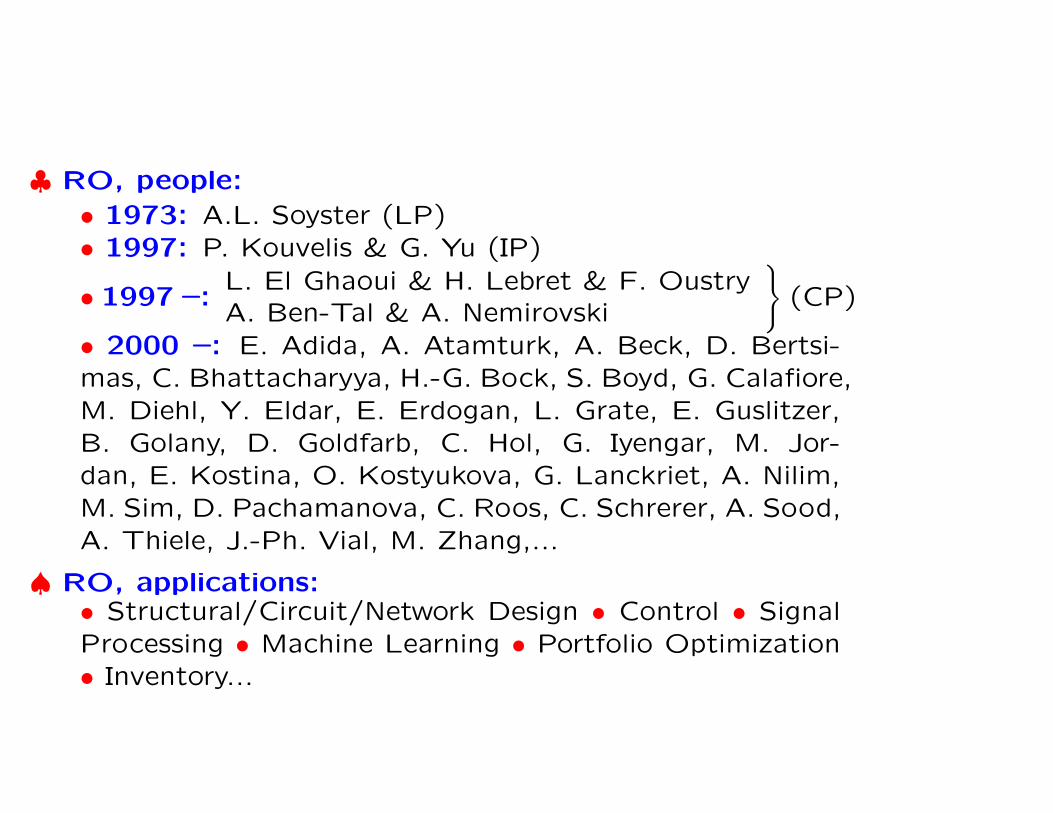
♣ RO, people:

• 1973: A.L. Soyster (LP)

• 1997: P. Kouvelis & G. Yu (IP)

• 1997 –:L. El Ghaoui & H. Lebret & F. OustryA. Ben-Tal & A. Nemirovski

}

(CP)

• 2000 –: E. Adida, A. Atamturk, A. Beck, D. Bertsi-

mas, C. Bhattacharyya, H.-G. Bock, S. Boyd, G. Calafiore,

M. Diehl, Y. Eldar, E. Erdogan, L. Grate, E. Guslitzer,

B. Golany, D. Goldfarb, C. Hol, G. Iyengar, M. Jor-

dan, E. Kostina, O. Kostyukova, G. Lanckriet, A. Nilim,

M. Sim, D. Pachamanova, C. Roos, C. Schrerer, A. Sood,

A. Thiele, J.-Ph. Vial, M. Zhang,...

♠ RO, applications:• Structural/Circuit/Network Design • Control • Signal

Processing • Machine Learning • Portfolio Optimization

• Inventory...

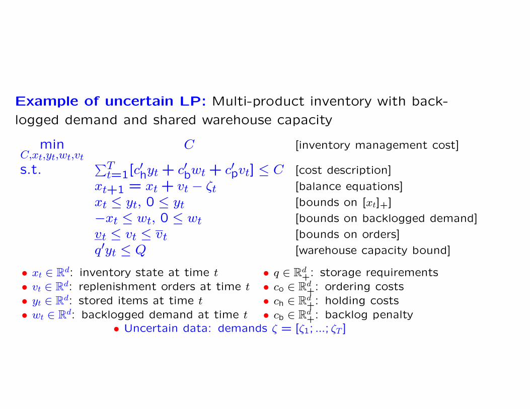
Example of uncertain LP: Multi-product inventory with back-

logged demand and shared warehouse capacity

minC,xt,yt,wt,vt

C [inventory management cost]

s.t.∑T

t=1[c′hyt + c′bwt + c′pvt] ≤ C [cost description]

xt+1 = xt + vt − ζt [balance equations]

xt ≤ yt, 0 ≤ yt [bounds on [xt]+]

−xt ≤ wt, 0 ≤ wt [bounds on backlogged demand]

vt ≤ vt ≤ vt [bounds on orders]

q′yt ≤ Q [warehouse capacity bound]

• xt ∈ Rd: inventory state at time t • q ∈ Rd+: storage requirements

• vt ∈ Rd: replenishment orders at time t • co ∈ Rd+: ordering costs

• yt ∈ Rd: stored items at time t • ch ∈ Rd+: holding costs

• wt ∈ Rd: backlogged demand at time t • cb ∈ Rd+: backlog penalty

• Uncertain data: demands ζ = [ζ1; ...; ζT ]

{

minx

{f(x, ζ) : F (x, ζ) ∈ K} : ζ ∈ Z}

(Unc)

Assume that our “decision environment” is such that

• All decisions xj should be made before ζ “reveals itself”

and thus should be independent of ζ

• The constraints are “hard”: their violations cannot be

tolerated

• We intend to take full care of all data ζ ∈ Z and do not

care what happens when ζ 6∈ Z.

Under these assumptions, seemingly the only meaningful way to

process (Unc) is to solve the Robust Counterpart

mint,x

{t : ∀ζ ∈ Z : f(x, ζ) ≤ t, F (x, ζ) ∈ K} (RC)

of the uncertain problem.

Example: To build the RC of the Inventory problem, we use

balance equations to eliminate the states and pass to the RC of

the resulting inequality constrained problem, thus arriving at

minC,yt,wt,vt

C

s.t.

∑Tt=1[c

′hyt + c′bwt + c′pvt] ≤ C

x1 +∑t−1

τ=1[vτ − ζτ ] ≤ yt, 0 ≤ yt

−x1 − ∑t−1τ=1[xτ − ζτ ] ≤ wt, 0 ≤ wt

vt ≤ vt ≤ vt, q′yt ≤ Q

∀ζ ∈ Z(RC)

Note: When Z is a computationally tractable convex set, the

semi-infinite problem (RC) is computationally tractable. E.g.,

when Z is polyhedral: Z = {ζ : ∃u : Pζ + Qu + r ≥ 0}, RC can

be converted into an explicit LP program of sizes polynomial in

T, d and the sizes of the representation of Z.

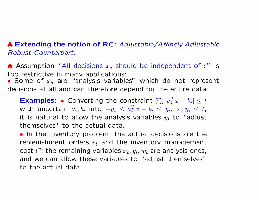
♣ Extending the notion of RC: Adjustable/Affinely Adjustable

Robust Counterpart.

♠ Assumption “All decisions xj should be independent of ζ” is

too restrictive in many applications:• Some of xj are “analysis variables” which do not represent

decisions at all and can therefore depend on the entire data.

Examples: • Converting the constraint∑

i |aTi x − bi| ≤ t

with uncertain ai, bi into −yi ≤ aTi x − bi ≤ yi,

i yi ≤ t,

it is natural to allow the analysis variables yi to “adjust

themselves” to the actual data.

• In the Inventory problem, the actual decisions are the

replenishment orders vt and the inventory management

cost C; the remaining variables xt, yt, wt are analysis ones,

and we can allow these variables to “adjust themselves”

to the actual data.

• In dynamical decision-making, some of the decisions xj should

be made when the actual data becomes partially known and thus

can depend on the corresponding portions of the data

Example: In the Inventory problem with uncertain de-

mand, replenishment orders vt of day t usually can depend

on the actual demands at days 1, ..., t − 1.

♣ To account for adjustability, we allow for every xj to depend

on a prescribed portion Pjζ of ζ: xj = Xj(Pjζ), thus arriving at

Adjustable Robust Counterpart

mint,{Xj(·)}n

j=1

{t : ∀ζ ∈ Z : f(X(ζ), ζ) ≤ t, F (X(ζ), ζ) ∈ K}

[X(ζ) = {Xj(Pjζ)}](ARC)

Note: ARC is infinite-dimensional and thus is typically heavily

computationally intractable. Seemingly the only applicable tech-

nique is Dynamic Programming ⇒“curse of dimensionality”

♣ To overcome, to some extent, intractability of ARC, we re-

strict the decision rules to be affine: Xj(Pjζ) = ξ0j + ξTj Pjζ, thus

arriving at the Affinely Adjustable Robust Counterpart

mint,{ξ0j ,ξj}n

j=1

{t : ∀ζ ∈ Z : f(X(ζ), ζ) ≤ t, F (X(ζ), ζ) ∈ K}

[X(ζ) = {ξ0j + ξTj Pjζ}n

j=1](AARC)

Example: The only “actual decisions” in the Inventory problemare orders vt. Assume that vt can depend on the precedingdemands ζt−1 = [ζ1; ...; ζt−1]. To build the AARC, we• introduce linear decision rules for the orders vt = v0

t + Vtζt−1

• make xt, yt, wt affine functions of ζ:xt = x0t + Xtζ, yt = y0

t +Ytζ, wt = w0

t + Wtζ, thus ending up with

minC,v0

t ,Vt,...,w0t ,Wt

C

s.t.

t≤T [c′h[y0t + Ytζ] + c′b[wt + Wtζ] + c′p[v

0t + Vtζt−1]] ≤ C

x0t+1 + Xt+1ζ = x0

t + Xtζ + v0t + Vtζt−1 − ζt

x0t + Xtζ ≤ y0

t + Ytζ, 0 ≤ y0t + Ytζ

−[x0t + Xtζ] ≤ w0

t + Wtζ, 0 ≤ w0t + Wtζ

vt ≤ v0t + Vtζt−1 ≤ vt, q′[y0

t + Ytζ] ≤ Q

∀ζ ∈ Z

(AARC)Note: The AARC of the Inventory problem is computationallytractable provided that Z is so. E.g., when Z is a polyhedral set,(AARC) is equivalent to an explicit LP program.

Example (continued): Consider single-product Inventory with

N = 10 and a box uncertainty set: (1 − ρ)ζn ≤ ζ ≤ (1 + ρ)ζn.

Here the ARC is well within the grasp of Dynamic Programming.

♣ How large are the gaps in the chain Opt(ARC) ≤ Opt(AARC) ≤Opt(RC) ?

• We built a sample of 768 Inventory problems with uncertainty

of 10% – 50% by picking at random cost coefficients, storage

capacity and nominal demand trajectory ζn and subsequent fil-

tering out problems with infeasible ARC’s.

♠ It turns out that Opt(ARC) = Opt(AARC) in every one of

these 768 problems!

Note: This phenomenon disappears when passing from minimiz-

ing the worst-case inventory management cost to minimizing the

average of this cost.

♠ Opt(RC) was typically essentially worse than Opt(ARC) =

Opt(AARC):

Range of Opt(RC)

Opt(ARC)1 (1,2] (2,10] (10,1000] ∞

Frequency in the sample 38% 23% 14% 11% 15%

♣ In the RO context, affine decision rules not necessarily are

bad!

• Optimization programs with uncertain data and theirRobust Counterparts

• Tractability of Robust Counterparts• Robust Optimization and Chance Constraints

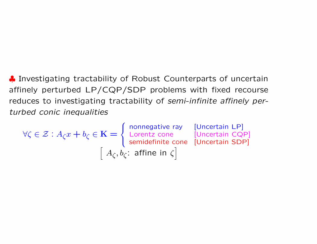
♣ Robust Counterparts of uncertain problem are semi-infinite

programs and thus can be intractable even when all instances of

the uncertain problem are easy to solve.⇒ When Robust Counterparts are computationally tractable?

What to do if it is not the case?

♠ We focus on uncertain affinely perturbed LP/CQP/SDP prob-

lems{

minx

{

cTζ x + dζ : Ai

ζx + biζ ∈ Ki, i = 1, ..., m

}

: ζ ∈ Z}

with fixed recourse:

• cζ, dζ, Aiζ, b

iζ: affine in ζ

• Fixed recourse [automatically valid for the RC]: All coeffi-

cients of the adjustable variables xj (those with Pj 6= 0) are

certain (i.e., independent of ζ).

• Ki: nonnegative rays/Lorentz cones/semidefinite cones (un-

certain LP, CQP, SDP, respectively).

♠ We always assume that Z is given by a strictly feasible semidef-

inite representation

Z = {ζ : ∃u : P(ζ, u) � 0}(P(·): affine in (ζ, u)).

♣ Investigating tractability of Robust Counterparts of uncertain

affinely perturbed LP/CQP/SDP problems with fixed recourse

reduces to investigating tractability of semi-infinite affinely per-

turbed conic inequalities

∀ζ ∈ Z : Aζx + bζ ∈ K =

nonnegative ray [Uncertain LP]Lorentz cone [Uncertain CQP]semidefinite cone [Uncertain SDP]

[

Aζ, bζ: affine in ζ]

♣ Tractability of a semi-infinite affinely perturbed conic inequal-

ity

∀ζ ∈ Z : Aζx + bζ ∈ K

depends on the tradeoff between the geometries of K and Z –

the more complicated is Z, the simpler should be K.

♣ “Trivial case”: Scenario-generated uncertainty set

Theorem. The RC/AARC of an uncertain affinely perturbed

LP/CQP/SDP problem{

minx

{

cTζ x + dζ : Ai

ζx + biζ ∈ Ki, i = 1, ..., m

}

: ζ ∈ Z}

with fixed recourse and with scenario-generated uncertainty set

Z = Conv{ζ1, ..., ζN} is computationally tractable.

♣ “Solvable case”: Uncertain LP

Theorem. The RC/AARC of uncertain affinely perturbed LP

problem{

minx

{

cTζ x + dζ : Ai

ζx + biζ ∈ Ki, i = 1, ..., m

}

: ζ ∈ Z}

[Ki : given by explicit lists of linear inequalities]

with fixed recourse is computationally tractable. With Z given by

a strictly feasible LP/CQP/SDP representation, the RC/AARC

is an explicit LP/CQP/SDP program of sizes polynomial in the

size of instances and the size of the representation of the uncer-

tainty set.

♣ Aside of a number of highly specific particular cases, semi-

infinite conic quadratic/linear matrix inequalities are computa-

tionally intractable. Whenever it is the case, a natural course

of actions in the RO context is to replace an intractable semi-

infinite conic inequality with its safe tractable approximation.

Definition. Consider a semi-infinite conic inequality

∀ζ ∈ Z : Aζx + bζ ∈ K (C)

and let 0 ∈ Z. We embed (C) into the parametric family of

semi-infinite conic inequalities

∀(ζ ∈ ρZ) : Aζx + bζ ∈ K (Cρ)

(ρ ≥ 0: uncertainty level).

A system of convex constraints (Sρ) in variables x and additional

variables u is called a safe tractable approximation of (Cρ) tight

within factor ϑ ≥ 1, if

• [tractability] The constraints in (Sρ) are efficiently computable

• [safety] Whenever x can be extended to a feasible solution of

(Sρ), x is feasible for (Cρ)

• [tightness] Whenever x cannot be extended to a feasible solu-

tion of (Sρ), x is not feasible for (Cϑρ).

♣ Safe tractable approximation of semi-infinite Conic Qu-

adratic Inequality

∀ζ = [ζ`; ζr] ∈ ρZ : ‖Aζ`x − bζ`‖2 ≤ cTζrx − dζr

[

Aζ`, bζ`, cζr, dζr are affine in ζ] (Cρ)

♠ (Cρ) is computationally tractable when:

• [simple ellipsoidal uncertainty] Z is an ellipsoid centered at the

origin

• [side-wise uncertainty with unstructured norm-bounded lhs per-

turbations] Z = Z` ×Zr, Z` = {ζ` ∈ Rp×q : ‖ζ`‖ ≤ 1} and

Aζ`x − bζ` ≡ P (x) + LT (x)ζ`R(x),

where P (x), L(x), R(x) are affine in x and either L(·), or R(·)are constant.

Example: The semi-infinite Least Squares inequality

∀(ζ ∈ Rp×q, ‖ζ‖ ≤ ρ) : ‖

[

[An, bn] + LT ζR]

[x; 1]‖2 ≤ t (Cρ)

admits exact SDP representation

tI − λLTL Anx + bn

λI ρR[x; 1]

[Anx + bn]T ρ[R[x; 1]]T t

� 0 (Sρ)

in variables t, x, λ: (t, x) is feasible for (Cρ) iff it can be extended

to a feasible solution to (Sρ).

∀ζ = [ζ`; ζr] ∈ ρZ : ‖Aζ`x − bζ`‖2 ≤ cTζrx − dζr (Cρ)

♠ (Cρ) admits tight tractable safe approximation when the

uncertainty is side-wise: Z = Z` ×Zr and

• [∩-ellipsoidal lhs perturbation set]

Z` = {ζ` : [ζ`]TQjζ` ≤ 1, 1 ≤ j ≤ M} with Qj � 0,

j Qj � 0

⇒(Cρ) admits an explicit safe SDP approximation tight within

the factor ϑ = O(1)√

lnM .

• [structured norm-bounded lhs perturbations]

Z` = {ζ` = {ζ`j}J

j=1 : ζ`j ∈ R

pj×qj : ‖ζ`j‖ ≤ 1}

Aζ`x − bζ` ≡ P (x) +∑

j LTj (x)ζ`

jRj(x)

where P (x), Lj(x), Rj(x) are affine in x and for every j either

Lj(·), or Rj(·) are constant.

⇒(Cρ) admits an explicit safe SDP approximation tight within

the factor ϑ = π2.

Example: [“Robust Least Squares Antenna/Filter Design”] The

semi-infinite Least Squares inequality

∀(ζ, ‖ζ‖∞ ≤ ρ) : ‖An(I + Diag{ζ})x − bn‖2 ≤ t (Cρ)

with “implementation errors xj 7→ (1 + ζj)xj” admits safe SDP

approximation

t − ∑

j λj [Anx − bn]T

Anx − bn tI ρAnDiag{x}ρ[AnDiag{x}]T Diag{λ1, ..., λn}

� 0 (Sρ)

which is tight within the factor π2.

♣ Safe tractable approximation of semi-infinite Linear Ma-

trix Inequality

∀(ζ ∈ ρZ) : Aζ(x) � 0[

Aζ(x) : bi-affine in x, ζ] (Cρ)

♠ Aside of scenario-generated uncertainty set, the only known

case when (Cρ) admits a tight tractable approximation is the

case of structured norm-bounded uncertainty:

Z = {ζ = {ζj}Mj=1 : ζj ∈ R

pj×pj , ‖ζj‖ ≤ 1, ζj = ξjI, j ∈ J}Aζ(x) = An(x) +

j

[

LTj ζjRj(x) + RT

j (x)ζTj Lj

]

[

An(x),Rj(x) are affine in x]

Theorem. The semi-infinite LMI

∀(

{ζj}Mj=1‖ζj‖ ≤ ρ ∀j, ζj = ξjIpj , j ∈ J

)

:

An(x) +∑

j

[

LTj ζjRj(x) + RT

j (x)ζTj Lj

]

� 0(Cρ)

with structured norm-bounded uncertainty admits a safe tractable

SDP approximation. The tightness factor ϑ of this approxima-

tion depends solely on the largest size of the scalar perturbation

blocks

µ =

{

1, J = ∅maxj∈J pj, J 6= ∅

and does not exceed ϑ(µ), where ϑ(·) is a universal function such

that ϑ(1) = π2, ϑ(2) = 2, ϑ(k) ≤ π

√k. In the case of M = 1 (single

perturbation block), the approximation is exact: ϑ = 1.

Applications in: Robust Structural Design, Lyapunov Stability

Analysis/Synthesis under interval uncertainty, etc.

• Optimization programs with uncertain data and theirRobust Counterparts

• Tractability of Robust Counterparts• Robust Optimization and Chance Constraints

♣ RO does not assume stochastic nature of uncertain data and

uses instead uncertain-but-bounded model of data perturbations.

However: Stochastic nature of uncertainty, if any, can be uti-

lized in the RO framework.

♣ Consider Uncertain LP with stochastic data. The entity of

primary interest here is a randomly perturbed linear constraint

w0(x) +∑d

`=1 ζ`w`(x) ≤ 0[

• x: decision vector • w0(x), ..., wd(x): affine• ζ1, ..., ζd ∈ R: “primitive” random perturbations

]

(C)

♠ A natural way to process (C) is to pass to a chance version

Prob{

w0(x) +∑d

`=1ζ`w`(x) > 0}

≤ ε (Cε)

of the constraint (A. Charnes, W. Cooper, G. Symonds, 1958).

π(w) ≡ Prob{ζw ≡ w0 +∑d

`=1 ζ`w` > 0} ≤ ε (Cε)

♠ There exists significant literature on chance constraints (T.

Badics, D. Dentcheva, A. Dupacova, L. Miller, A. Prekopa, A.

Ruszczynski, B. Vizvari, H. Wagner,...)

However: In general, (Cε) is difficult to process:

• In many cases, the feasible set of a chance constraint is non-

convex;

• Even when convex, the feasible set of (Cε) can be “computa-

tionally intractable”:

When ζ ∼ Uniform([0,1]d), π(w) is quasi-convex (C. Lagoa et al.,

2005). However, unless P=NP, it is impossible to compute π(w)

with accuracy δ > 0 in time polynomial in d, total binary length of

(rational) w and ln(1/δ) [L. Khachiyan, 1989].

π(w) ≡ Prob{ζw ≡ w0 +∑d

`=1 ζ`w` > 0} ≤ ε (Cε)

♣ When (Cε) “as it is” is difficult to process, one can look

for a safe tractable approximation of (Cε) – a computationally

tractable convex set Wε such that

Wε ⊂ {w : π(w) ≤ ε} (∗)♠ A way to build a safe tractable approximation of (Cε):

Take a convex function γ : R → R with lims→−∞

γ(s) = 0,

γ(0) = 1 and set Γ(w) = E {γ(ζw)} .Note: π(w) ≤ Γ(αw) ∀α > 0 and Γ(·) is convex, whence

the set Wε = cl {w : ∃α > 0 : Γ(αw) ≤ ε} is convex and

satisfies (∗).

⇒Whenever Γ(·) is efficiently computable, Wε is a safe tractable

approximation of (Cε).

γ(·) : R → R+, γ(0) = 1 : convex, lims→−∞

γ(s) = 0

⇒ Γ(w) ≥ E

{

γ(

w0 +∑d

`=1 ζ`w`

)}

: convex

⇒ Wε ≡ cl {w : ∃α > 0 : Γ(αw) ≤ ε}⊂{w : Prob{ζw > 0} ≤ ε}Note: Wε is a closed convex cone such that

Wε = {w ∈ Rd+1 : w0 +

∑d

`=1ζ`w` ≤ 0 ∀ζ ∈ Zε}

for an appropriate convex compact set Zε.

⇒The safe approximation w(x) ∈ Wε of the chance constraint

Prob{w0(x) +∑d

`=1 ζ`w`(x) > 0} ≤ ε

is nothing but the Robust Counterpart

∀ζ ∈ Zε : w0(x) + ζ1w1(x) + ... + ζdwd(x) ≤ 0

of the uncertain affinely perturbed linear constraint

w0(x) + ζ1w1(x) + ... + ζdwd(x) ≤ 0

with properly defined perturbation set Zε.

♣ How to choose γ(·)?♠ As far as the conservatism of the upper bound

Prob{ζw > 0} ≤ infα>0

E{γ(ζαw)}[γ(·) ≥ 0 : convex nondecreasing, γ(0) = 1]

is concerned, the best choice of γ(·) is γ(s) = max[1 + s,0].

This choice leads to the famous Conditional Value at Risk safe

approximation

minβ∈R

[

β +1

εE{[ζw − β]+}

]

︸ ︷︷ ︸

CVaRε(w)

≤ 0

of the chance constraint

Prob{ζw > 0} ≤ ε.

However: Typically, CVaRε(·) is difficult to compute...

♣ Ensuring computability: Bernstein approximation [Pin-

ter, 1989; Nem.&Shapiro, 2005]

Observation: Consider a chance constraint

Prob{w0 +∑d

`=1 ζ`w` > 0} ≤ ε (Cε)

and assume that

• ζ1, ..., ζd are independent

• We are smart enough to build efficiently computable

convex bounds Φ`(r) ≥ ln(

E{erζ`})

on the logarithmic

moment-generating functions of ζ`, ` = 1, ..., d.

Choosing γ(s) = es, one can set

Γ(w) = exp{w0 +∑d

`=1 Φ`(w`)}thus arriving at a tractable safe approximation of (Cε).

Example (one of many): Range and mean a priori information

on ζ`. Consider a chance constraint

Prob{w0(x) +∑d

`=1 ζ`w`(x) > 0} ≤ ε

• ζ` ∈ [−1,1]: independent • E{ζ`} ∈ [µ−` , µ+

` ](Cε)

The associated Bernstein approximation of (Cε) is

∀ζ ∈ Zε : w0(x) +∑d

`=1 ζ`w`(x) ≤ 0,

Zε = {ζ :∑d

`=1 φ`(ζ`) ≤ 2 ln(1/ε)}

φ`(s) =

(1 + s) ln(

1+s1+µ−

`

)

+ (1 − s) ln(

1−s1−µ−

`

)

,−1 ≤ s ≤ µ−`

0 , µ−` ≤ s ≤ µ+

`

(1 + s) ln(

1+s1+µ+

`

)

+ (1 − s) ln(

1−s1−µ+

`

)

, µ+` ≤ s ≤ 1

(Br)

∀ζ ∈ Zε : w0(x) +∑d

`=1 ζ`w`(x) ≤ 0,

Zε = {ζ :∑d

`=1 φ`(ζ`) ≤ 2 ln(1/ε)}, φ`(s) = ...︸ ︷︷ ︸

“Entropy uncertainty”, Nem.&Shapiro, 2006

(Br) ⇔ Explicit CP

⇓Prob{w0(x) +

∑d`=1 ζ`w`(x) > 0} ≤ ε (Cε)

• ζ` ∈ [−1,1]: independent • E{ζ`} ∈ [µ−` , µ+

` ]

♠ (Br) can be further safely approximated by

∀ζ ∈ Z+ε : w0(x) +

` ζ`w`(x) ≤ 0

Z+ε = {‖ζ‖∞ ≤ 1}⋂

[

{‖ζ‖2 ≤√

2 ln(1/ε)}+{µ− ≤ ζ ≤ µ+}

]

︸ ︷︷ ︸

“Ball-Box uncertainty”, Ben-Tal & Nem., 2000

(BB) ⇔ Explicit CQP

∀ζ ∈ Z+ε : w0(x) +

` ζ`w`(x) ≤ 0

Z+ε = {‖ζ‖∞ ≤ 1}⋂

[

{‖ζ‖2 ≤√

2 ln(1/ε)}+{µ− ≤ ζ ≤ µ+}

](BB) ⇔ Explicit CQP

⇓∀ζ ∈ Zε : w0(x) +

∑d`=1 ζ`w`(x) ≤ 0,

Zε = {ζ :∑d

`=1 φ`(ζ`) ≤ 2 ln(1/ε)}, φ`(s) = ...(Br) ⇔ Explicit CP

⇓Prob{w0(x) +

∑d`=1 ζ`w`(x) > 0} ≤ ε (Cε)

• ζ` ∈ [−1,1]: independent • E{ζ`} ∈ [µ−` , µ+

` ]

♠ (BB) is further safely approximated by

∀ζ ∈ Z++ε : w0(x) +

` ζ`w`(x) ≤ 0

Z++ε = {‖ζ‖∞ ≤ 1}

⋂[

{‖ζ‖1 ≤√

2d ln(1/ε)}+{µ− ≤ ζ ≤ µ+}

]

︸ ︷︷ ︸

“Budgeted uncertainty”, Bertsimas & Sim, 2003

(Bd) ⇔ Explicit LP

∀ζ ∈ Z : w0(x) +∑d

`=1 ζ`w`(x) ≤ 0 (RC[Z])⇓

Prob{w0(x) +∑d

`=1 ζ`w`(x) > 0} ≤ ε (Cε)

• ζ` ∈ [−1,1]: independent • E{ζ`} ∈ [µ−` , µ+

` ]

d = 64 d = 128 d = 256

Random 2D cross-sections of Entropy (red), Ball-Box (yellow)

and Budgeted (green) uncertainty sets, ε = 0.005, µ±` = 0.

Black: cross-section of the support {‖ζ‖∞ ≤ 1} of ζ.


Recommended