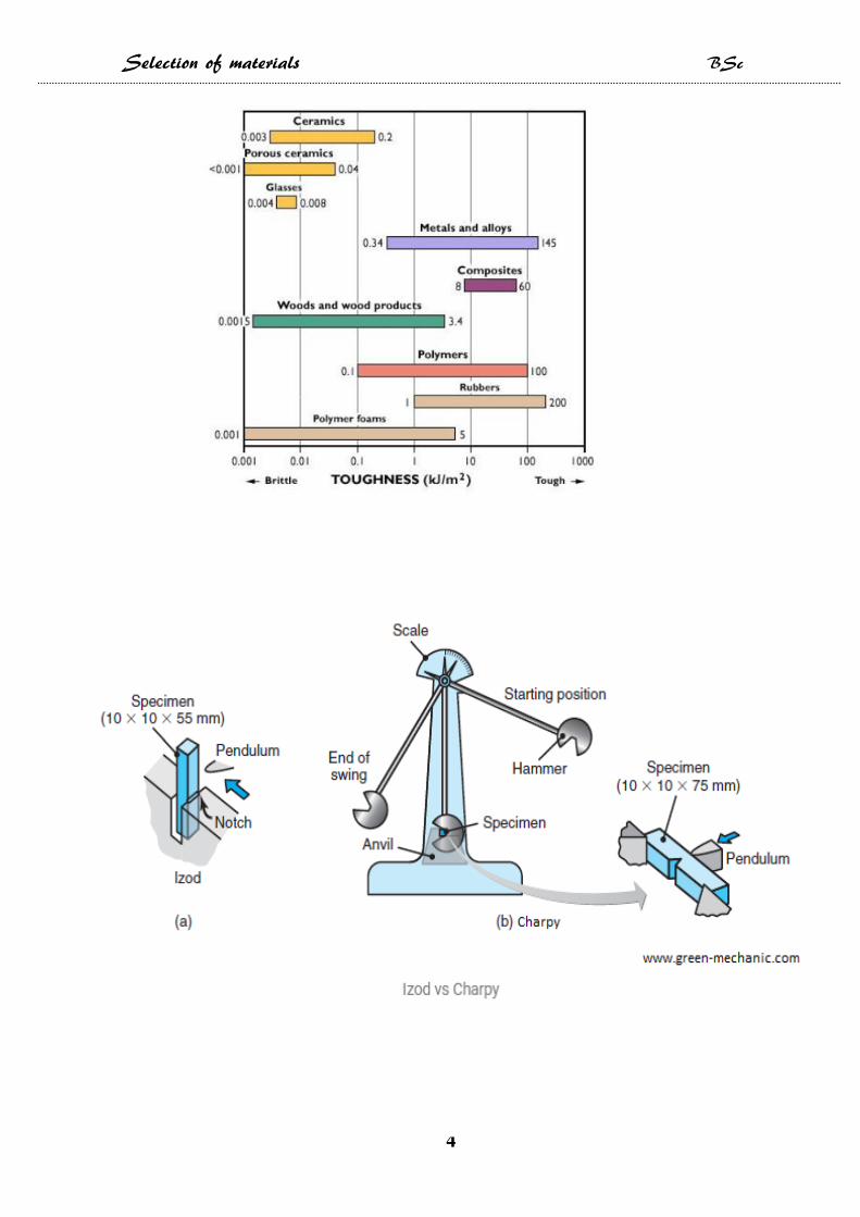
Selection of materials BSc 1 Toughness is the ability of a material to absorb energy and plastically deform without fracturing. One definition of material toughness is the amount of energy per unit volume that a material can absorb before rupturing. It is also defined as a material's resistance to fracture when stressed. Toughness requires a balance of strength and ductility Toughness can be determined by integrating the stress-strain curve. It is the energy of mechanical deformation per unit volume prior to fracture. The explicit mathematical description is:
Transcript
Selection of materials BSc
1
Toughness is the ability of a material to absorb energy and plastically
deform without fracturing. One definition of material toughness is the
amount of energy per unit volume that a material can absorb
before rupturing. It is also defined as a material's resistance
to fracture when stressed.
Toughness requires a balance of strength and ductility
Toughness can be determined by integrating the stress-strain curve. It is
the energy of mechanical deformation per unit volume prior to fracture.
Fracture toughness is an indication of the amount of stress required to
propagate a preexisting flaw. Flaws may appear as cracks, voids,
metallurgical inclusions, weld defects, design discontinuities, or some
combination thereof. Since engineers can never be totally sure that a
material is flaw free, it is common practice to assume that a flaw of some
chosen size will be present in some number of components and use the
linear elastic fracture mechanics (LEFM) approach to
design critical components. A parameter called the stress-
intensity factor (K) is used to determine the fracture
toughness of most materials.
Where( Y) is a dimensionless geometry factor on the order of 1, (σc )
is the stress applied at failure, and (a) is the length of a surface crack
(or one-half the length of an internal crack).
(KIC) are MPa.m1/2.
The fracture toughness (KIC) is the critical
value of the stress intensity factor at a crack tip
needed to produce catastrophic failure under
simple uniaxial loading. The subscript I stands for
Mode I loading (uniaxial), illustrated in figure a
while the subscript C stands for critical. The
fracture toughness is given by:
Selection of materials BSc
6
which provides values for KIC under “plane strain” conditions,
meaning that (Note B=t= thickness) :
, where t is the sample thickness.
Example: Estimate the flaw size responsible for the failure of a turbine
motor made from partially stabilized Aluminum oxide that fractures at a
stress level of 300 MPa .
Selection of materials BSc
7
Solution :
From table, KIC =2.7 MPa.m1/2
------
-------
Selection of materials BSc
8
Viscoelastic materials
Almost, all materials possess viscoelastic properties, and operate differently
in tensile and compression strength and loading styles. Viscoelasticity in
polymer is more sensible than metals. That is, deformation in polymer is not
only a function of applied load, but it also depends on time (loading rate). The
materials which their deformation depends on time, as viscoelastic materials,
have both solid and fluid like behaviors. Linear viscoelasticity is often used
successfully for describing the real behavior in case of small or moderate loads.
The use of thermoplastics in structural applications demands accurate design
data that spans appropriate ranges of stress, strain rate, time and temperature.
In polymeric materials, the primary molecular chains are held together by
weak cohesive forces. These chains are constantly rearranging their
configurations by random thermal motion. The driving force for these motions
is the thermal energy contained in the system .When subjected to an external
stress. rearrangement on a local scale takes place rapidly but that on a larger
scale occur rather slowly. This in turn leads to a wide range of time spans
where changes in mechanical properties are observed. This behavior is termed
viscoelasticity. the amount of crystalinity. cross-linking and chain structure also
affects the overall behavior . Using polymer, instead of metal, is increasingly
being developed. The vast differences between polymer and metal properties
and some disadvantages like polymer’s higher viscoelasticity than metal, which
results in creep and relaxation behavior in polymer, it’s very lower elasticity
modulus and low fracture stress than metal, high thermal expansion coefficient
(which is 10 times more than metals), low dimensional stability.
Viscoelasticity is the study of materials which exhibit features of both elastic
and viscous behavior. Elastic materials deform instantaneously when a load is
applied, and remembers its original conjuration, returning there
Selection of materials BSc
9
instantaneously when the load is removed. A mechanical model representing
this can be seen by observing a spring.
On the other hand, viscous materials do not show such behavior, instead they
exhibit time dependent behavior. While under stress, a viscous body strains at
a constant rate, and when its load is removed, the material fails to return to its
initial conjuration. A mechanical model of a viscous material can be seen by
observing a dash-pot. Viscoelastic materials exhibit the combined
characteristics of both elastic and viscous behavior, resulting in partial
recovery. A mechanical model of viscoelastic behavior can be represented by
various combinations of spring and dash-pot elements in series or parallel.
Figure shows the standard viscoelastic response of polymers undergoing creep
and stress relaxation. By analyzing the creep modulus and relaxation modulus,
further insight may be gained regarding the viscoelastic behavior of polymers.
The Creep behavior of viscoelastic materials
The creep phenomena is defined as a slow continuous deformation over time
at constant load . Creep is an important consideration in the design. However, the
processes of creep can be subdivided and examined into the three of categories
primary creep, tertiary creep and steady state creep . The processes are illustrated
in figure and are explained below:
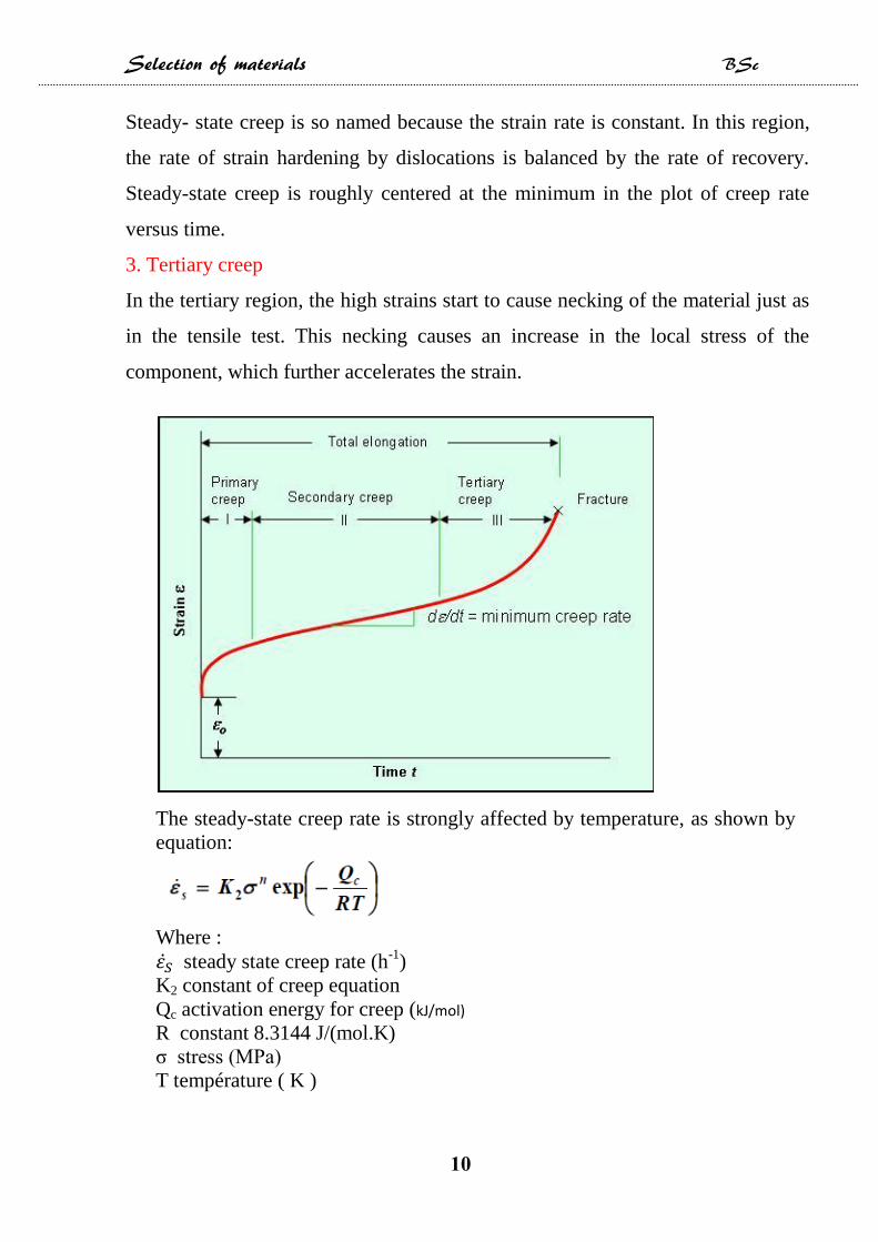
1.Primary creep
During primary creep, the strain rate decreases with time until a constant rate is
reached. And this tends to occur over a short period. Primary creep strain is
usually less than one percent of the sum of the elastic, steady state, and primary
strains. The mechanism in the primary region is the climb of dislocations that are
not pinned in the matrix.
2. Steady state creep
Selection of materials BSc
11
Steady- state creep is so named because the strain rate is constant. In this region,
the rate of strain hardening by dislocations is balanced by the rate of recovery.
Steady-state creep is roughly centered at the minimum in the plot of creep rate
versus time.
3. Tertiary creep
In the tertiary region, the high strains start to cause necking of the material just as
in the tensile test. This necking causes an increase in the local stress of the
component, which further accelerates the strain.
The steady-state creep rate is strongly affected by temperature, as shown by
equation:
Where :
steady state creep rate (h-1
)
K2 constant of creep equation
Qc activation energy for creep (kJ/mol)
R constant 8.3144 J/(mol.K)
σ stress (MPa)
T température ( K )
Selection of materials BSc
11
Example
Steady-state creep data for an alloy at 200ºC yield:
The activation energy for creep is known to be 140 kJ/mol. What is the steady-state creep rate at 250ºC and 48 MPa? Sol :
Now we can subtract these to yield:
Notice that because T1 = T2, the last term cancels out. Substituting in the data that was given:
n = 9.97 K2= 3.27χ10-5 (h-1)
Selection of materials BSc
12
Relation between materials and activation energy
Relation between materials and Creep
The temperature at which materials start to creep depends on their melting
point. As a general rule, it is found that creep starts when
where TM is the melting temperature in kelvin. However, special alloying
procedures can raise the temperature at which creep becomes a problem.
Polymers, too, creep — many of them do so at room temperature.
Selection of materials BSc
13
Selection of materials BSc
14
The Larson-Miller parameter is a means of predicting the lifetime of
material vs. time and temperature
Creep-stress rupture data for high-temperature creep-resistant alloys are often plotted as log stress to rupture versus a combination of log time to rupture and temperature. One of the most common time–temperature parameters used to present this kind of data is the Larson-Miller (L.M.) parameter, which in generalized form is
T = temperature, K tr = stress-rupture time, h C = constant