Self-Inflicted Unemployment Scarring and Stigma * Julien Hugonnier 1,4,5 , Florian Pelgrin 2,6 , and Pascal St-Amour 3,4,6 1 ´ Ecole Polytechnique F´ ed´ erale de Lausanne 2 EDHEC Business School 3 HEC Lausanne, University of Lausanne 4 Swiss Finance Institute 5 CEPR 6 CIRANO August 15, 2019 * We have benefited from very useful discussions with and comments from Rob Alessie, Marnix Amand, Tony Berrada, David Card, Rafael Lalive, Lars Ljungqvist, Fabien Postel-Vinay, Jean-Marc Robin, Bruce Shearer and Nicolas Werquin, as well as from participants at the IZA World Labor 2018 Conference and the Society of Labor Economists 2017 Annual Meeting. Financial support from the Swiss Finance Institute is gratefully acknowledged. The usual disclaimer applies.
Transcript
Self-Inflicted Unemployment Scarring and Stigma∗
Julien Hugonnier1,4,5, Florian Pelgrin2,6, and Pascal St-Amour3,4,6
1Ecole Polytechnique Federale de Lausanne
2EDHEC Business School
3HEC Lausanne, University of Lausanne
4Swiss Finance Institute
5CEPR
6CIRANO
August 15, 2019
∗We have benefited from very useful discussions with and comments from Rob Alessie, Marnix Amand,
Tony Berrada, David Card, Rafael Lalive, Lars Ljungqvist, Fabien Postel-Vinay, Jean-Marc Robin, Bruce
Shearer and Nicolas Werquin, as well as from participants at the IZA World Labor 2018 Conference and
the Society of Labor Economists 2017 Annual Meeting. Financial support from the Swiss Finance
Institute is gratefully acknowledged. The usual disclaimer applies.
Abstract
Long-term scars of unemployment include higher ex-post displacement and lower
re-employment likelihoods, as well as income losses that increase in occurrence and
duration of previous unemployment spells. Human capital explanations assume
that its accumulation is valued by the market, but is impaired by non-employment.
We retain the former assumption, yet relax the latter by considering continuous
investment decisions made by workers across employment statuses, where wages,
as well as likelihood and duration of unemployment spells are capital-dependent.
We calculate analytically the joint optimal investment by the employed and the
unemployed. We structurally estimate the model using NLSY79 data and identify
two dynamically stable steady-state values with a lower one for the unemployed.
Circular dynamics follow whereby human capital optimally falls during unemploy-
ment spells and increases again upon re-employment. Scarring and stigma are thus
self-inflicted, i.e. endogenously induced through decisions made by agents only. A
counter-factual exercise allows to gauge and confirm the importance of employment
risks hedging in total demand for human capital and that of moral hazard issues
in the design of UIB programs. We also show that status-dependent accumulation
technology and capital specificity complement, but are not required for scarring
and stigma.
Keywords— Human capital; Unemployment; Duration dependence; unem-
ployment stigma and scarring; Displacement; Re-employment probability; Simu-
lated Moments Estimation.
JEL classification— J24, J64, J65
1 Introduction
1.1 Motivation and overview
In addition to contemporaneous income losses associated with incomplete and temporary
replacement,1 unemployment (u) imposes long-term costs to workers. On the one hand,
scarring refers to persistent detrimental labor market outcomes, such as earnings decline,2
as well as lower employment (e), re-employment (u → e) and higher displacement (e →
u) probabilities of workers with previous unemployment spells.3 On the other hand,
negative duration dependence (stigma) implies more unfavorable ex-post outcomes the
longer agents are not working.4 Despite being persistent, unemployment scars and stigma
are not permanent, with more distant spells having weaker effects than recent ones.5
Human capital is often invoked as an explanation for unemployment scarring and
stigma. This conjecture relies on two postulates: (i) human capital is valued by employers
1The U.S. weighted average UI replacement rate in 2010-2011 was 0.41 and varied between 0.30(AK, LA) and more than 0.49 (AZ, HI, RI) with median maximal duration of 26 weeks. Source: U.S.Department of Labor.
2Jacobson et al. (2005, Fig. 1) report that pre- vs post-displacement earnings losses are 10% for short-tenured, 23% for medium-tenured and 30% for long-tenured workers. See Kletzer (1998); Arulampalamet al. (2001); Abbott (2008); Quintini and Venn (2013); Carrington and Fallick (2014) for reviews of USand international evidence on post-unemployment income losses. Additional discussion of income scarsis presented in Jacobson et al. (1993); Neal (1995); von Wachter et al. (2009); Farber (2011); Davis andvon Wachter (2011); Fang and Silos (2012); Huckfeldt (2016). Corresponding welfare costs are found tobe substantial by Rogerson and Schindler (2002); Krebs (2007).
3Ruhm (1991a) finds that displacement entails a three times higher risk of future unemployment.Stevens (1997) shows that displacement induces multiple additional displacement, resulting in long-termearnings losses. Krueger et al. (2014, Fig. 3) show that the long-term unemployed (> 26 weeks) have anexit rate to employment less than half that of the very short-term (< 5 weeks). Guvenen et al. (2017)emphasize the persistence of (voluntary and involuntary) non-employment statuses in explaining earningslosses. Fujita and Moscarini (2017) distinguish between recalled and new hires in analyzing e → u → etransitions, showing that recalled workers had more tenure, received offers faster and stayed longer withtheir employer, while experiencing more duration dependence than new hires. See also Nilsen and Reiso(2011); Eliason and Storrie (2006) for Scandinavian and Arulampalam (2001) for British evidence onemployment scarring. Seniority rules determining Last-in-First-Out termination policies are discussedin Kletzer (1998); Medoff and Abraham (1981); Carmichael (1983).
4Kroft et al. (2013) rely on fictitious CV’s sent to prospective employers advertising openings and findthat call-backs were 45% lower for 8-month unemployment spells, compared to 1-month. Similar effectsthrough low call-backs are identified in Eriksson and Rooth (2014) for Swedish data. See also Eubanksand Wiczer (2016); Alvarez et al. (2016); Nekoei and Weber (2015); Huttunen et al. (2011); van denBerg and van Ours (1996); Ruhm (1991b) for discussions of the role of sample composition effects andunobserved heterogeneity in explaining duration dependence.
5See Jacobson et al. (2005); Davis and von Wachter (2011); Carrington and Fallick (2014) fordiscussions.
and (ii) its accumulation is impaired by non-employment. Evidence for capital valuation
include higher wages, lower displacement risk and faster re-employment transitions for
skilled workers.6 Reasons for slower capital accumulation for the unemployed include
not learning-by-doing, faster skills depreciation and less efficient learning technologies
in non-employment, as well as human capital specificity, technological obsolescence, and
unemployment insurance (UI) incentives distortions. The relative depreciation of the
unemployed workers’ capital is sanctioned by employers who rely on observable spell
occurrence and duration as a screening mechanism to identify existence and magnitude
of imperfectly observed human capital losses. Firms are consequently less willing to hire
and pay high wages to, as well as are more inclined to lay off previously unemployed
workers, especially the long-duration ones.
Our main research question is whether these long-term unemployment costs are still
relevant when we retain assumption (i) of valuable capital, but when we abstract from
assumption (ii) of exogenous accumulation wedges across employment statuses. In partic-
ular, we ask whether unemployment scarring and stigma can persist an environment where
measurable human capital (i) is associated with both a lower likelihood and expected
duration of unemployment spells, in addition to higher wages and (ii) can be continuously
adjusted by agents in both employment and unemployment states. Whereas the first
assumption is well justified empirically and in the literature, the second postulate can
be rationalized by invoking workers’ decisions at the extensive (i.e. participation) and
intensive (i.e. effort) margins with respect to on-the-job training, continuing education
and active UI programs.7 To the extent that capital positively affects wages, as well as
reduces unfavorable employment risks and that its accumulation is decided by the agent,
exposure to unemployment scarring and stigma should be minimized by investing more
6See Mincer (1974) for education, tenure and experience gradients of wages. See Neal (1995); Kletzer(1998); Farber (2005, 2011); Riddell and Song (2011); Gomes (2012); Fang and Silos (2012); Quintiniand Venn (2013) for evidence on role of human capital in mitigating exposure to labor market risks,
7Evidence and theoretical rationalization for human capital decision- and cost-sharing in employmentare provided by Becker (1962, 1993); Acemoglu and Pischke (1999); Fu (2011); Marotzke (2014); Krakel(2016) whereas unemployed agents’ participation in active UI policies is reviewed by Heckman et al.(1999); Jacobson et al. (2005).
2
when employed (to prevent displacement), as well as when unemployed (to accelerate
re-employment and counter duration dependence). If the optimal strategy nonetheless
admits long-term unemployment costs, then any residual scarring and stigma must be
optimally self-inflicted by the agent.
To answer this question, we address unemployment scarring and stigma through the
lens of classical Human Capital (HK) investment theory, to which we append endogenous
exposure to employment risks. We rely on four modeling choices. First, we take as
primitive the assumption that human capital induces better wages, as well as lower
displacement risk and faster re-employment transitions for the better-skilled agents.
Second, we internalize both the income and employment risks motives in a HK setup with
Ben-Porath (1967) accumulation featuring stochastic employment states and endogenous
transition densities. Third, a realistic specification of unemployment insurance benefits
provides both the resources and the incentives for investing during unemployment spells.
Finally, we allow for (but do not impose) differences in human capital technology across
employment statuses, as well as for firm- or sector-specific capital losses incurred upon
occurrence of displacement. Abstracting from both in our baseline setup lets us emphasize
scarring dynamics resulting from optimal investment policies, instead of from arbitrary
parametric restrictions, such as less efficient capital accumulation, or faster depreciation
rates for the unemployed. We later reinstate status-dependent technology and capital
specificity to gauge their respective contributions.
We compute interior investment rules for this problem and characterize the wages and
employment dynamics resulting from the optimal choices. Solving this dynamic model
is particularly challenging for two reasons. First, as is the case for Diamond (1982);
Mortensen and Pissarides (1994) (DMP) Search and Matching models – and unlike
standard HK models –, the employment and unemployment value functions are non-
separably intertwined with one another, as the returns to investing when employed depend
on what is selected when unemployed and vice versa. Second and more importantly,
both the displacement and re-employment arrival rates are endogenous functions of
3
the human capital decided by the agent, which enriches the motives for investing, but
significantly complicates the model’s solution. We circumvent this problem through two-
step expansion methods developed in Hugonnier, Pelgrin and St-Amour (2013). We start
by solving analytically a restricted version (referred to as order-0) where the arrival rates
governing displacement and re-employment are exogenously set. We then do an expansion
on this solution (order-1) where the perturbation concerns the key parameter governing
the endogeneity of the arrival rates.
We first show that the order-0 solution yields two separate and constant human capital
growth, such that no steady-state exists. Consequently, the exogenous employment risks
case captures only a subset of the stylized facts on scarring and stigma. To illustrate its
shortcomings, we abstract from ad-hoc depreciation and productivity differences across
employment statuses, as well as from capital specificity in our baseline scenario. A
high capital gradient of income is then sufficient to yield lower investment and growth
for the unemployed than for the employed. Since capital positively affects employment
revenues, the gap in constant growth rates generates positive income wedges that are
increasing in unemployment occurrence and duration, consistent with income scarring
and stigma. However, constant growth rates levels and differentials entail permanent
effects of unemployment, at odds with the persistent, but temporary nature of observed
scarring and stigma. Moreover, because displacement and re-employment intensities are
exogenously set and cannot be adjusted, slower capital growth during unemployment
spells is inconsequential for future employment risks exposure. The restricted model is
thus unable to reproduce employment scarring and stigma observed in the data.
We next reinstate endogenous displacement and re-employment intensities in calculat-
ing the order-1 solutions to assess whether these shortcomings can be addressed. The as-
sociated human capital, employment and income dynamics are significantly more complex
to investigate analytically and we resort to numerical analysis instead. For that purpose,
we structurally estimate the order-1 model using a Simulated Moments Estimation (SME)
to match predicted and observed employment and income dynamics from NLSY79 data.
4
Again abstracting from technological differences and capital specificity, our baseline
results confirm that the optimal human capital dynamics are now fully consistent with
both income and employment scarring and stigma, as well as with their non-permanent
features. This finding rests on two main results. First, investment by the unemployed is
positive, but lower than for the employed. Second, two distinct employed and unemployed
steady-state levels of human capital exist, are both dynamically stable, and with a lower
steady state for the unemployed. Combining the two results entails circular optimal
wages and risks dynamics. Upon unemployment, human capital optimally falls towards
the lower unemployed steady state and increases towards the higher employed steady
state upon re-employment. Since re-employment (resp. displacement) and wages are
recall rates and lower wages and higher displacement upon re-employment (scarring).
Moreover, since human capital falls continuously until either re-employment occurs or the
steady state is reached, duration dependence (stigma) obtains internally. Because scarring
and stigma depend on displacement and re-employment events whose joint likelihood is
human capital-dependent and since the investment in the capital is decided by workers
exclusively, scarring and stigma are self-inflicted in the sense that both arise through an
optimal dynamic strategy of workers, with minimal and realistic assumption on market
valuation of skills, and abstracting from heterogeneous technology across statuses.
We next rely on a counter-factual exercise to assess the various mechanisms at play.
First, since our model innovates from standard human capital theory in that particular
dimension, we gauge the importance of displacement and re-employment risks control in
total demand for human capital. By removing endogenous exposure and adjusting the
parameters to maintain the mean displacement/reemployment rates constant, we show
that the marginal effects of risk exposure adjustment strongly complements any wage
considerations in investment decisions. Second, we also measure the policy effects of UI
generosity and of base income on total investment. Standard search models associate
more generous programs with reduced search efforts and longer unemployment spells
5
(e.g. Chetty, 2008; Daly et al., 2012). We offer an alternative moral hazard explanation
whereby less generous UIB increases the motives for investing, decreasing unemployment
through lower displacement and higher re-employment. Finally, our baseline results
assume employment status independent technologies and no capital specificity. We assess
the importance the these restrictions by re-introducing both in turn. Our results show
that unemployment disadvantages are complementary, but not necessary for self-imposed
scarring and stigma to occur.
This paper contributes to discussions of human capital in labor market dynamics.
We highlight the importance of endogenous employment risks exposure as additional
motivation for investing in one’s own human capital as a complement to the traditional
higher wages argument. These employment risks are widely assumed to be the result
of systemic macro shocks and cannot be insured against through market instruments,
thereby justifying both active macro stabilization and UIB policies. We show instead
that displacement and re-employment risks can be adjusted through agents’ decisions
and that long-term scars can nonetheless obtain optimally through investment choices
made by workers only. Finally, we highlight the strong moral hazard risks in making the
UIB programs more generous. This results in lowering the incentives for investing, with
ensuing higher displacement and lower wages and re-employment.
1.2 Related literature
HK models Our paper is most directly related to the HK literature where agents make
continuous decisions on their human capital accumulation subject to Ben-Porath (1967)
technology. A first strand emphasizes the role of specificity, of capital complementarities
and of market frictions in optimal cost- and decision-sharing by workers and firms (Becker,
1962, 1993; Acemoglu and Pischke, 1999; Fu, 2011; Marotzke, 2014; Krakel, 2016). A
second strand focuses on heterogeneity in human capital production, both in terms
of abilities and in types of acquired capital (Ingram and Neumann, 2006; Cunha and
Heckman, 2007; Heckman, 1976, 2008; Hu and Taber, 2011; Yamaguchi, 2012; Polachek
6
et al., 2015; Jones, 2014; Stantcheva, 2017; Guvenen et al., 2018). A third subset
of HK contributions is primarily concerned with the life cycle of wages and earnings,
notably how pre-employment education, finite employment and life horizons reduces
human capital investment late in life and yields hump-shaped earnings profiles (Heckman,
1976, 2008; Keane and Wolpin, 1997; Huggett et al., 2006, 2011; Cervellati and Sunde,
2013; Hendricks, 2013; Kredler, 2014; Fan et al., 2015). A fourth strand of the HK
literature measures the impact of non-diversifiable depreciation and income shocks to the
accumulation process (Rogerson and Schindler, 2002; Krebs, 2003; Pavoni, 2009; Huggett
et al., 2011).
We follow the classical HK approach in letting capital investment decisions be made
and costs be incurred by agents exclusively. In addition, the model is flexible enough
to allow for differences in abilities or technology, as well as between general and specific
capital. However, we do not emphasize heterogeneity in the primitives as the main
driving force. Rather heterogeneous income and employment outcomes stem exclusively
from optimal investment and idiosyncratic shocks whose distributions are endogenously
determined through the agents’ choices. Moreover, although the HK framework we resort
to is by definition a life cycle model, we do not emphasize its life cycle properties. In
particular, we neither focus on education decisions made prior to labor market entry, nor
do we rely on the earnings profile by age to identify the properties of the human capital
dynamics. Finally, the distribution of human capital shocks found in the literature is
exogenously set and cannot be altered by the agent’s decisions. One exception is Keane
and Wolpin (1997) where agents select between finite alternative distributions on human
capital returns. However, our choices are continuous, rather than among a fixed set of
alternatives (e.g. working, not working) and the shocks we consider are exclusively driven
by changes in employment status whose transition matrix is human capital-dependent.
DMP models Our paper is more indirectly related to the strand of the DMP Search
and Matching models either explictly or implicitly emphasizing human capital (DMP-
7
HK). Explicit DMP-HK literature8 primarily adopts a learning-by-doing perspective
whereby skills reflect work experience that improve match quality and wages and that
accumulate if employed and stagnate or decline during non-employment spells (either
voluntary or not). Human capital accumulation in DMP-HK models is best characterized
as a by-product of workers’ job acceptance decisions and on- and off-the-job search efforts,
rather than as a consequence of explicit investment choices by agents.9 Exposure to
employment risk is also indirectly affected by workers decisions, such as in the case of
endogenous separation, where matches are not consumed in light of insufficient ex-post
quality (Esteban-Pretel and Fujimoto, 2014; Fujita and Moscarini, 2017) or in unemploy-
ment search efforts that are combined with market tightness conditions (Mukoyama et
al., 2018), as well as human capital specificity (Fujita and Moscarini, 2017; Fujita, 2018)
to determine the job arrival rate.
We also draw from the DMP literature with implicit references to human capital.
For example, the match quality in Pissarides (1992) depends on past employment sta-
tus and is higher for previously employed workers, thereby mimicking additional skills
depreciation during unemployment. Recall models such as Fujita and Moscarini (2017)
emphasize dynamics for match productivity that persist as long as a worker does not
find employment outside a given firm, thereby capturing firm-specific human capital that
can be drawn upon when recalled. Kroft et al. (2016) implicitly mimic unemployment
depreciation by directly appending negative duration dependence to model UE transitions
in a search framework. Finally, Job Ladders models (Lise, 2013; Pinheiro and Visschers,
8Examples of DMP settings with explicit human capital considerations include Ljungqvist and Sargent(1998); Shimer and Werning (2006); Pavoni (2009); Yamaguchi (2010); Burdett et al. (2011); Esteban-Pretel and Fujimoto (2014); Bagger et al. (2014); Ortego-Marti (2017); Fujita (2018); Guvenen et al.(2018). Capital depreciation can further be accelerated in “micro-turbulent” periods where workers sufferfrom specific skills obsolescence (Ljungqvist and Sargent, 1998; Kitao et al., 2017).
9Exceptions in DMP-HK setups with explicit investment decisions include Flinn and Mullins (2015)who consider binary schooling choices made prior to market entry and Kitao et al. (2017) who allow fordirect investment at the mid-life (Experienced) phase. Flinn et al. (2017); Fu (2011) analyse joint trainingdecisions by workers/employers, whereas agents decide on job offers that include training opportunities,as well as wages, whereas Lentz and Roys (2015) consider training decisions made by firms exclusively.Guvenen et al. (2018) let workers select accumulation through directional search for firms with differentskills requirements that augment human capital. This literature considers income motives only foraccumulation, with no effects on the distribution of employment risks internalized in workers decisions.
8
2015; Moscarini and Postel-Vinay, 2016; Krolikowski, 2017) emphasize slow resolution
of mismatches between demanded and offered skills to explain wages and employment
risks dynamics. These papers have implicit references to human capital where displaced
workers suffer from jumps to less favorable employment ladders and slowly climb back
up when their capital is replenished following re-employment.
We indirectly borrow from the DMP paradigm in letting agents’ decisions affect
their employment outcomes and from the DMP-HK segment by channeling this influence
through their human capital. We also implicitly assume that match quality is improved
by the latter, resulting in better employment opportunities (wages/risks) for high-capital
agents. Moreover, the circular optimal wage and employment dynamics we uncover share
strong similarities with those obtained under the Job Ladders approaches.
However, several differences with DMP are worth mentioning. First, we abandon the
learning-by-doing perspective by making capital accumulation a product of deliberate
and continuous decisions by agents across both the employment and the unemployment
statuses. Equivalently, whereas DMP models focus on extensive margin adjustments
associated with changes in statuses, we emphasize intensive adjustments where agents can
continuously fine-tune their human capital throughout the employment or unemployment
spells. Second, we depart from DMP in taking a partial-equilibrium and agents-focused
perspective. Unlike the latter, firms act mechanically in our setup, supplying the wage,
displacement and re-employment functions that are taken as primitives and are not
stemming from general equilibrium. Finally, we put forward an idiosyncratic, rather
than systemic stochastic environment where the capital-induced distributions are agent-
specific and do not encompass equilibrium variables such as the market tightness rate.
2 NLSY79 evidence on scarring and stigma
We resort to National Longitudinal Survey of Youth (NLSY79) data to provide prima
facie evidence of scarring and stigma, as well as to compute empirical moments that
9
are relied upon in the Simulated Moments Estimation below. NLSY79 is a widely-used10
panel of 9,964 respondents aged between 14-22 in 1979, and followed up to 2014, providing
longitudinal information on employment statuses and income, as well on socio-economic
variables (see Appendix A for details). Summary statistics in Table 1 shows that our
sample is evenly balanced on gender, composed mainly of white, US citizens, of average
age 32, and living in urban areas. Human capital measures include close to 13 years of
highest completed grade, with 14% of respondents indicating vocational or professional
training. Labor market experience shows that 91% were employed with mean income less
than 17 K$ in real terms.
Table 2 identifies employment scarring and stigma by reporting current employment
probabilities by past statuses (panel a) and by human capital (panels b and c). First,
t−1 unemployment lowers current employment by 26.4% (95.13%-68.73%), whereas t−2
unemployment reduces it by 17.2% (78.25%-95.44%). Duration dependence (stigma)
is apparent as being continuously unemployed in the last two periods reduces current
employment by 38.7% (96.31%-57.58%).
Second, panels b and c show the mitigating effects of human capital on unemployment
level and persistence. Agents with less than high school had 14.3% (97.70%-83.39%) lower
employment rates in general compared with those having college degree. They also faced a
30.9% (89.36%-58.43%) lower employment if previously unemployed, compared with only
a 8.9% (97.96%-89.07%) gap for those with college degrees. Vocational and professional
training also provides some attenuating effects, although of lower magnitude compared to
education. Trained agents had higher employment by 2.7% (95.15%-92.46%), and faced
a past unemployment gap of 24.0% (96.75%-72.77%), compared with 28.1% (94.82%-
66.72%) for untrained respondents.
Table 3 reveals similar scarring and stigma when measured in terms of income.
Declining persistence is visible with t−1 unemployment resulting in 64.7% lower income,
while t−2 spells lower income by 52.2%. Income stigma is also apparent with continuous
10See Guvenen et al. (2018); Lise (2013) and references therein for recent applications.
10
unemployment in the last two periods leading to a 74.2% drop in current revenues.
The mitigating human capital effect on income is less striking compared to that on
employment. Although college graduates earn 61.8% more than those without high
school, the effects of education on the income gap associated with t − 1 unemployment
is relatively constant, ranging between 57.3% and 61.6%. Again, the effect of training
appears more limited.
These statistical findings are confirmed by longitudinal regression analysis. Table 4
shows the marginal effects from panel Probit regressions of current employment statuses,
controlling for socio-demographic characteristics and year fixed effects. The dependent
variables are (1) the unconditional, i.e. Pr(et), (2) re-employment, i.e. Pr(et | ut−1)
and (3) continuing employment, i.e. non-displacement Pr(et | et−1). First, in panel a,
past employment statuses improve current employment, re-employment and continuing
employment. The temporary nature of scarring is apparent with weaker effects associated
with time t− 2 statuses, compared to t− 1. Second, in panel b, human capital measured
either through lagged work experience (i.e. cumulated past statuses up to t−1), education
or training significantly augment current employment, re-employment, and continuing
employment probabilities. Table 5 makes similar findings for current income via panel
GLS, random-effects regressions. Positive gradients are also found for being employed in
the last two periods, with stronger effects for more recent statuses. Again, human capital
proxied by work experience, education, or training improve current, re-employment, and
continuing employment incomes.
Overall, we conclude that the employment and income scarring costs associated with
previous unemployment are significant, as well as compounded by duration (stigma),
and are more important for recent than for distant spells. Human capital augments both
employment and income and is a significant hedge against these scarring and stigma costs.
The next section describes a theoretical model incorporating these elements. Consistent
with Tables 4, and 5, we assume that labor demand values human capital with higher re-
employment, lower displacement probabilities, as well as higher wages. Taking these labor
11
market characteristics as given, we let agents select their investment in human capital
and verify whether the resulting dynamics are consistent with scarring and stigma costs
identified with NLSY79 data.
3 HK Model with Endogenous Employment Risks
Exposure
Overview Consider an economy where agents are characterized by two sources of
heterogeneity: Human capitalHt ∈ R+ and labor market status it ∈ {e, u} (i.e. employed,
unemployed). The former is defined as the publicly measurable set of skills accumulated
by workers over their lifetime. We assume that investment in human capital is decided
by agents and takes place both within (e.g. through experience or voluntary training)
and outside (e.g. through formal and informal education) employment. The pecuniary
(e.g. tuition fees, books, software, . . . ) and indirect (e.g. opportunity cost of time and
effort spent acquiring skills) investment costs are borne by individuals. Human capital
provides no direct utility flows to the agent, but is valued by employers, as reflected
in more favorable conditions with respect to wages, firing and hiring for highly-skilled
agents. Although our perspective is on general human capital, we allow for part of that
capital to be immediately depreciated upon a displacement event in order to reflect firm-
or industry-specific components that have limited value to outside employers.
Labor market statuses are stochastic and the transition matrix between employment
and unemployment spells is agent-specific, in that it depends on the accumulated level of
human capital. Employed agents receive an income that is continuously adjusted to reflect
changes in human capital. Conversely, unemployed agents receive unemployment benefits
that are set at a fraction of the last employment revenue; the benefits are constant for the
duration of the unemployment spell. Risk-neutral agents thus select optimal investment
paths taking into account its joint benefits in terms of income premia and employment
risk adjustments.
12
Employment statuses A person’s time-t labor market status it follows a Poisson
stochastic process. Importantly, the arrival intensity is assumed to be dependent of the
observable human capital level Ht. More specifically, let T i, be the random time of job
displacement from current employment (e → u = i), or re-employment from current
unemployment (u→ e = i), with Poisson arrival intensities λi : R+ → R++ defined as:
λi(Ht) = limτ→0
1
τPr[t < T i < t+ τ | Ht
], i ∈ {e, u}
= λi0 + λi1H−ξit , λi0, λ
i1 ≥ 0; ξi > −1. (1)
Equivalently, the time t probability of remaining employed (e 6→ u = i) or remaining
unemployed (u 6→ e = i) up to t+ s is therefore:
Pt[T i > t+ s
]= exp
[−∫ t+s
t
λi(Hτ )dτ
], i ∈ {e, u}.
Imposing ξu > 0 in (1) entails decreasing and convex work displacement intensities,
Figure 1. An agent can thus reduce his exposure to conditional employment risks by
investing in his human capital which decreases his displacement intensity λu(H), as well
as increases his re-employment intensity λe(H). On the one hand, the parameters λi0
represent unadjustable exposure to displacement and re-employment hazard. On the
other hand, the parameters λi1 capture the endogeneity of the employment risks exposure
and play a key role in the solution method discussed below, with ξi governing the extent
of diminishing returns to investment against employment shocks.
13
Figure 1: Re-employment and Displacement Intensities
λe(H)
λu(H)
H
λi(H) = λi0 + λi1H−ξit
λe0
λu0
Notes: λe(H): re-employment intensity. λu(H): displacement intensity. H: human
capital
Income process The income process Yt = Y (Ht, H, it) ∈ R+ is status- and human-
capital-dependent:
Y (Ht, H, e) = Y e(Ht) = y0 + y1Ht, (2a)
Y (Ht, H, u) = Y u(H) = ηY e(H), (2b)
where η ∈ (0, 1) is the UI replacement rate and where H is the last measurable human
capital level at the beginning of the unemployment spell (i.e. lock-in capital).
Figure 2 shows that employment income Y e(H) increases in human capital which
can be continuously altered through the agent’s investment decisions. Upon job loss
at human capital level H0, unemployment income at point b is a fraction η of the last
employment income Y u(H) = ηY e(H0) and remains fixed throughout the duration of the
unemployment spell. For example, if human capital declines to H1 during unemployment,
UI income remains constant, whereas the income upon re-employment income at point d is
lower than previously, Y e(H1) < Y e(H0). Consistent with passive UI policies, investment
14
Figure 2: Employed and Unemployed Income
Y e(H) = y0 + y1H
Y u(H) = ηY e(H)
H
Y i(H)
H = H0H2
Y e(H0)
y0
H1
Y e(H1)
a
e b
d
c
Notes: Y e(H): Employed income. Y u(H): Unemployed income at replacement rate
η, evaluated at last measurable capital H.
decisions during the unemployment spell thus affect the displacement and re-employment
probabilities, as well as the re-employment wage, but not the UI benefits.11
Note further that the income loss (resp. gain) associated with displacement (resp.
re-employment):
∆Y (H,H) = Y e(H)− Y u(H)
= (1− η)y0 + y1(H − ηH) (3)
is an increasing function of H and can become negative if human capital depreciates
sufficiently during the unemployment spell, i.e. for H < H2 in Figure 2. Indeed, beyond
point e, UIB benefits are more generous than what would be earned upon re-employment,
thereby lowering incentives to invest in order to augment re-employment probability.
11See St-Amour (2015) for an alternative UIB policy with continuous adjustments in Y u(H) = ηY e(H),instead of lock-in capital. The results for this specification are qualitatively similar.
15
Human capital dynamics The law of motion for the agent’s human capitals, dHt =
dHt(It, Ht, it), is status-dependent and is given by:
The accumulation process (4) is in the spirit of the HK literature, (e.g. Ben-Porath,
1967; Heckman, 1976; Huggett et al., 2006; Kredler, 2014) and captures continuous, as
opposed to period-specific (e.g. pre-employment education) investment It decided by the
agent. The Cobb-Douglas gross investment function P iIαt H1−αt dt is monotone increasing
and concave in its arguments. The productivity term P i can be equivalently interpreted
as an ability or as the inverse of an investment price, whereas depreciation δi can be
interpreted as technological obsolescence of acquired skills.
Unlike most models who assume on-the-job training only (i.e. It(it = u) ≡ 0),
or active unemployment training decided by UI planners (e.g. Spinnewijn, 2013), the
agent’s investment decisions span across employment statuses. Differences in productivity
and depreciation capture status-dependent returns to investment. For example, faster
depreciation, and/or lower productivity when unemployed12 can be attained by imposing
δu > δe and P u < P e. Conversely, a lower opportunity cost of time spent on It for
the unemployed obtains through P u > P e. We remain agnostic by not imposing such
restrictions and instead solving the model for any δi, P i combinations.
The literature also puts forward distinctions between general and firm- or industry-
specific human capital, where the latter has a lower outside value (Hamermesh, 1987;
Becker, 1993; Neal, 1995; Ljungqvist and Sargent, 1998; Wasmer, 2006; Decreuse and
Granier, 2013). We can incorporate this feature by defining a transferability share
φ ∈ (0, 1] representing the general capita. In the spirit of Ljungqvist and Sargent (1998),
a newly displaced agent’s capital is thus only valued φHt < Ht to prospective employers
for income and reemployment intensity purposes. This non-stochastic jump can capture
12See Pissarides (1992); Acemoglu (1995); Ljungqvist and Sargent (1998); Pavoni and Violante (2007);Pavoni (2009); Spinnewijn (2013) for discussions of unemployment disadvantages in capital accumulation.
16
firm- or industry-specific capital that is foregone when employment is terminated. Alter-
natively, the loss (1− φ)Ht can also be interpreted as discrimination or branding against
unemployed workers whereby the actual capital is under-estimated by prospective employ-
ers following an unemployment spell. Both the effects on displacement/re-employment
and on firm-specific capital loss are fully internalized in the agent’s investment decisions,
as will be seen below.
Preferences All agents are infinitely-lived13 and select dynamic investment in human
capital It to maximize the expected discounted (at rate ρ) value of net income flow,
taking as given the dynamics for human capital, the distributional assumptions and
income function. More specifically, the value function can be written as:
V (H0, H, i0) = supI
E0
∫ ∞0
e−ρt[Y (Ht, H, it)− It
]dt ≥ 0, (5)
subject to the intensities (1), the income rate (2) and the human capital law of motion (4).
We remain in the HK tradition in assuming risk-neutral preferences in (5), with two
important implications. First, observe that negative net income Yt − It < 0 always
remains feasible and can be achieved by implicit borrowing (at rate r = ρ), as long as the
expected net present value V (H0, H, i0) remains non-negative.14 Second, risk neutrality
implies that any incremental demand for human capital (above that related to higher
income) induced by endogenous displacement and re-employment risks cannot strictly be
justified by self-insurance motives. Rather, this demand stems from a duration service
whereby human capital augments the expected time spent in the employed state (with
associated high income Y e(H)), and reduces that spent in unemployment (with associated
low income Y u(H)). Observe that this duration service comes at no extra cost (aside from
13In the spirit of the Perpetual Youth literature, the model is easily adaptable to finite lives is easilyby assuming Poisson death intensity λm and augmenting discounting at rate ρ + λm over an infinitehorizon (e.g. Blanchard, 1985).
14St-Amour (2015) considers the case where risk-averse agents have no access to borrowing for humancapital investment. The main findings obtained through numerical solutions remain qualitatively similarto the ones of this paper.
17
the increase in marginal price due to convex adjustment costs) and can thus be interpreted
as positive side benefit of investment over and above income considerations.
Letting V e(H), V u(H,H) denote the pair of value functions and invoking the Law
of Iterated Expectations with Poisson distributions allows the agent’s problem (5) to be
written as a joint optimization system:
V e(H0) = supI
∫ ∞0
e−∫ t0 (ρ+λ
u(Hs))ds [Y e(Ht)− It + λu(Ht)Vu(φHt, Ht)] dt, (6a)
V u(H0, H) = supI
∫ ∞0
e−∫ t0 (ρ+λ
e(Hs))ds[Y u(H)− It + λe(Ht)V
e(Ht)]
dt. (6b)
The presence of V u(φH,H) in the employed agent’s problem (6a) highlights the additional
depreciation that is associated with employment-specific capital (1−φ)H that is foregone
upon the displacement event occurring with intensity λu(Ht). The UI income in (6b) is
calculated at locked-in capital H until re-employment occurs with intensity λe(Ht), after
which the agent returns to V e(H). The program (6) features endogenous discounting at
augmented rates ρ+ λi(H) induced by the Poisson distributional assumption.
The corresponding Hamilton-Jacobi-Bellman (HJB) representation of (6) is:
0 = supI− ρV e(H)− λu(H) [V e(H)− V u(φH,H)] + Y e(H)− I
+ V eH(H)
[−δeH + P eIαH1−α] ,
0 = supI− ρV u(H,H)− λe(H)
[V u(H,H)− V e(H)
]+ Y u(H)− I
+ V uH(H,H)
[−δuH + P uIαH1−α] .
18
Calculating the first-order conditions and substituting back into the objective function
reveals that the joint HJB system simplifies to:
0 =− ρV e(H)− λu(H) [V e(H)− V u(φH,H)] + Y e(H) (7a)
− δeHV eH(H) + (1− α)α
α1−αH [P eV e
H(H)]1
1−α ,
0 =− ρV u(H,H)− λe(H)[V u(H,H)− V e(H)
]+ Y u(H) (7b)
− δuHV uH(H,H) + (1− α)α
α1−αH
[P uV u
H(H,H)] 1
1−α .
The bi-variate system of first-order differential equations (7) has no analytical solution
due to the endogeneity and nonlinear functional forms used for the intensity functions (1).
St-Amour (2015) relies on Chebyshev polynomials to calculate numerical solutions to
a similar program. We resort instead to a two-step approximate closed-form solution
method developed in Hugonnier, Pelgrin and St-Amour (2013). First we remove the
endogeneity in the employment intensities by imposing λi1 = 0 in (1). This exogenous
employment risks case yields a closed-form solution (referred to as order-0 solution) for
V i0 (H,H), I i0(H,H). Second, we rewrite the endogenous intensity component as λi1 =
ελi
1, i = e, u for some constants λi
1 and perturbation ε and perform a first-order expansion
of the value functions around the ε = 0 solution:
V e(H, ε) ≈ V e(H, 0) + εV eε (H, 0), (8a)
V u(H,H, ε) ≈ V u(H,H, 0) + εV uε (H,H, 0). (8b)
Once the approximate solution (referred to as order-1) for the value functions is obtained,
any relevant associated variable such as investment and human capital growth is thus
recovered through a similar expansion (see Hugonnier et al., 2013, for details).
Remark 1 (baseline scenario) In order to emphasize capital dynamics resulting from
optimal investment, rather than from technological differences, it will also be useful to
define a baseline scenario of status-independent technologies, and no capital specificity:
19
δi = δ, P i = P, i ∈ {e, u} (9a)
φ = 1. (9b)
Our theoretical results of Section 4 will be obtained for the general case of status-
dependent (δi, P i) and specificity φ ∈ (0, 1], while our simulated results of Sections 5
and 6 will focus on the baseline scenario (9), before reintroducing technological differences
and specificity in Section 7.
4 Optimal human capital investment and growth
We now calculate the optimal investment, starting first with the exogenous displace-
ment and re-employment (order-0), followed by the more general case where both are
endogenous (order-1).
4.1 Exogenous displacement and re-employment (order-0)
Theorem 1 (exogenous employment risks) Let λe1 = λu1 = 0 and assume that the
order-0 transversality and regularity conditions conditions (16) in Appendix C hold. Then:
1. The indirect utility functions of employed and unemployed agents are given as:
V e0 (H) = Ae0 + AehH (10a)
V u0 (H,H) = Au0 + AuhH + AubH (10b)
2. The optimal investment functions are given as:
Ie0(H) = H (P eαAeh)1
1−α (11a)
Iu0 (H) = H (P uαAuh)1
1−α (11b)
20
3. The optimal human capital growth functions are given as:
ge0 = −δe + P e 11−α (αAeh)
α1−α (12a)
gu0 = −δu + P u 11−α (αAuh)
α1−α (12b)
where the parameters (Ae, Au) are given in closed form in Appendix D.
First, the last measurable human capital level before the unemployment spell begins
H is valued under unemployment in (10b), but not for employed agents in (10a). Indeed,
the UIB program sets H = H when unemployment begins, such that the value function
simplifies to a function of H only from the employed agent’s perspective. Second,
the optimal investment in (11) shows that the investment-to-capital ratio is constant.
Consequently, so are the the growth rates (12) such that no steady-state exists at the order
zero. The expressions Aih in the indirect utility (10), investment (11), and growth (12)
functions capture the status-dependent shadow prices, i.e. the Tobin’s marginal-q’s of
human capital, that jointly solve (20). Corollary 1 in Appendix D shows that a sufficiently
high income gradient y1 in (2) results in a lower Tobin’s-q for the unemployed, Auh < Aeh.
For the baseline scenario in (9), it follows from (12) that the growth rate of human
capital is then always lower for the unemployed, i.e. gu0 < ge0. This special case is useful
to illustrate the shortcomings of the exogenous exposure to employment risks solved in
Theorem 1.
Indeed, Figure 3 plots the corresponding optimal evolution of ht = ln(Ht) for agents j, k
with identical initial level at t0, and with both employed up to t1. Whereas agent j is
continuously employed at all periods, agent k becomes unemployed at t1 and has his
human capital grow at lower rate (in red) gu0 < ge0. If re-employed at t2, his human
capital grows at the same rate ge0 as agent j (in blue), but its level is permanently lower
by distance f−c. A second unemployment spell at t3 results in the same lower unemployed
growth rate as at t1, and permanently lower human capital by amount h − e following
re-employment at t4.
21
Figure 3: Permanent scarring and stigma with exogenous employment risks
ht = ln(Ht)
t3
hj,t
hk,t
t2t1 t4t0
ge0
gu0
a
b
c
de
f
g
h
1
1
Notes: Optimal log human capital dynamics (employed: blue; unemployed: red),
exogenous displacement and re-employment case λe1 = λu1 = 0, assuming condition (21)
in Corollary 1 and for baseline scenario (9).
Permanent human capital wedges translate into permanent income wedges in (2), that
are increasing in both occurrence and duration of unemployment spells (see Figure 3).
Constant growth rates differentials predicted by the exogenous employment risks model
thus imply permanent, duration-dependent, income scarring of unemployment, contrary
to observed patterns of persistent, but temporary, and duration-dependent income wedges
(e.g. Jacobson et al., 2005; Davis and von Wachter, 2011; Carrington and Fallick, 2014).
Relaxing the baseline scenario (9) to allow for status-dependent technologies and speci-
ficity will have quantitative, but not qualitative effects; except in the unlikely case where
parameters are such that gu0 = ge0, income scars increase in spell duration and are not
mean-reverting. Moreover, because the order-zero case imposes λi1 = 0 in (1), the human
22
capital wedges in Figure 3 are inconsequential for post-unemployment displacement and
re-employment risks exposure. A second shortcoming of the restricted case is therefore
that unemployment episodes have no impact on the likelihood and duration of future
unemployment spells. To summarize, the exogenous employment risks model case can
generate income scarring and stigma, but fails to account for the non-permanent nature
of these costs, and is unable to generate employment scarring and stigma.
4.2 Endogenous displacement and re-employment (order-1)
We now consider the more general case of endogenous exposure to gauge whether the
shortcomings of the exogenous employment risks exposure model can be addressed.
Theorem 2 (endogenous employment risks) Assume that the order-0 transversality
and regularity conditions conditions (16) in Appendix C hold. Then, up to a first-order
approximation,
1. The indirect utility functions of employed and unemployed agents are given as:
V e(H) =V e0 (H) +Be
uλu1H−ξu +Be
1uλu1H
1−ξu +Beeλ
e1H−ξe
+Be1eλ
e1H
1−ξe ,
(13a)
V u(H,H) =V u0 (H,H) +Bu
uλu1H−ξu +Bu
1uλu1H
1−ξu +Bue λ
e1H−ξe
+Bu1eλ
e1H
1−ξe +BubHλ
e1H−ξe ,
(13b)
2. The optimal investment functions are given as:
Ie(H) =Ie0(H) + Ceuλ
u1H−ξu + Ce
1uλu1H
1−ξu + Ceeλ
e1H−ξe
+ Ce1eλ
e1H
1−ξe ,
(14a)
Iu(H,H) =Iu0 (H) + Cuuλ
u1H−ξu + Cu
1uλu1H
1−ξu + Cue λ
e1H−ξe
+ Cu1eλ
e1H
1−ξe + CubHλ
e1H−ξe .
(14b)
23
3. The optimal human capital growth functions are given as:
ge(H) =ge0 +Deuλ
u1H−1−ξu +De
1uλu1H−ξu +De
eλe1H−1−ξe
+De1eλ
e1H−ξe ,
(15a)
gu(H,H) =gu0 +Duuλ
u1H−1−ξu +Du
1uλu1H−ξu +Du
eλe1H−1−ξe
+Du1eλ
e1H−ξe +Du
bHλe1H−1−ξe .
(15b)
where the order-0 values V e0 (H), V u
0 (H,H), Ie0(H), Iu0 (H,H) and ge0(H), gu0 (H,H) are given
in Theorem 1 and where the parameters (Be, Bu), (Ce, Cu) and (De, Du) are given in
closed form in Appendix E.
When contrasted with Theorem 1, the order-1 results of Theorem 2 show that the
investment shares of human capital I i(H,H)/H are no longer constant. It follows that
neither are the optimal growth functions gi(H,H), such that steady state values H iSS(H)
may exist, contrary to the exogenous employment risks case. Importantly, generalizing
λi1 6= 0 permits feedback effects of changes in H for employment risks exposure. In
addition to income wedges identified for the order-0 case, any gaps in the optimal
dynamics ge(H) − gu(H,H) will be penalized in both displacement and re-employment
intensities, thereby reinstating potential employment scarring and stigma.
5 Simulated human capital dynamics
The investment and growth functions revealed by the order-1 optimal rules in Theorem 2
are much more challenging to describe analytically than their order-0 analogs. We
therefore resort to numerical analysis to identify the dynamics of employment statuses
and income induced by those of the human capital. Again to emphasize optimal evolution
of Ht, rather than parametric choices, we first evaluate the model for the baseline
scenario (9). We will reinstate both status-dependent technology and firm-specific capital
loss in the comparative statics exercise in Section 7.
24
5.1 Simulated Moments Estimation
SME procedure We rely on Simulated Moments Estimation15 to structurally estimate
a large subset of the model’s main parameters corresponding to the displacement and re-
employment intensities parameters (λi, ξi) in (1), the income process (y0, y1) in (2), as
well as the human capital dynamics parameters (δ, α) in (4). The other parameters such
as the UI replacement rate (η) and the discount rate (ρ) are set at standard value. The
productivity parameter (P i) is calibrated relying on thorough search procedure, while the
capital specificity (φ) is set at one in our baseline setup and is varied in the sensitivity
analysis below.
The estimation is implemented so as to match the theoretical moments calculated
from the simulated histories of employment statuses and incomes (ij, Yij ) = {ij,t, Y i
j,t}Tt=1
to their NLSY79 counterparts. The moments to be matched are the unconditional, con-
ditional and joint (i.e. continuation) moments for employment and income. We minimize
the optimally-weighted square distance between observed and predicted moments, where
the estimation is undertaken subject to the three order-0 transversality and regularity
conditions conditions (16) in Appendix C.
Simulation Our model simulation follows the Monte Carlo procedure outlined in Ap-
pendix F. For a given set of structural parameters, conditional on status it = e, u, current
Ht and locked-in capital H t, the optimal investment I i(Ht, H t) from Theorem 2 are
selected, and the Poisson intensities λi(Ht) are determined. The agent’s status and
capital are then updated to (it+1, Ht+1), with special provision – when applicable – for a
share (1−φ) of employment-specific capital being lost upon new displacement events, and
the Poisson intensities are updated as well to λi(Ht+1). The procedure is iterated upon
over j = 1, 2, . . . , 5’000 individuals and for T = 100 periods, with the initial (burn-in)
draws t ∈ [1, 50] discarded for moments calculations.
15See McFadden (1989); Duffie and Singleton (1993); Newey (2001) for theoretical SME considerationsand French (2005); French and Jones (2011); Boyd et al. (2013); Pelgrin and St-Amour (2016) forapplications.
25
5.2 Results
Moments matching and parameters Table 6 reports the observed and theoretical
moments. The unconditional, conditional and joint employment moments in panel (a)
are very well reproduced, whereas those associated with income in panel (b) are less so.
In particular, the employed and unemployed income levels are correctly fitted, but the
effects of past employment histories on income tend to be understated, suggesting other
income factors not accounted for by the model. Notwithstanding these caveats, the overall
SME fit for the joint employment and income moments can be considered as adequate,
which is remarkable considering the spartan assumptions of the model, especially with
the baseline restrictions (9) imposed.
Table 7 presents the estimated SME (standard errors in parentheses) and calibrated
(no std. err.) parameters. The former are all estimated precisely. Importantly, both the
λi1 and ξi parameters in panel a are significantly different from zero at the 1% level, thereby
rejecting the null of the exogenous risks model in Section 4.1 in favor of the endogenous
displacement and re-employment model of Section 4.2. Similarly, y1 is significant in
panel b, consistent with a valuation of human capital in the income function. Finally,
the estimated law of motion (4) parameters are in the habitual range of estimates for
Ben-Porath (1967) technology and indicative of diminishing returns in investment.16
Optimal investment Figure 4 plots the SME-consistent estimates of the optimal
investment in human capital for the employed (in blue, LHS scale) and unemployed (in
red, RHS scale) agents, in function of H and for mid-level H lock-in capital level. First,
we find that investment for unemployed agents is lower for all H and H compared to
employed workers. Second, investment is falling in human capital for the employed, but
is U-shaped for the unemployed due to conflicting income and employment risks effects.
Indeed, on the one hand, increasing H reduces the likelihood of displacement, while
increasing the re-employment probability, thereby reducing the incentives for investment.
16Estimates for α vary between 0.35 and 0.80, whereas δ estimates range between 0.027 and 0.07 (seethe references cited in Polachek et al., 2015, p. 1425).
26
Diminishing returns in adjusting the arrival intensities λi(H) entail that the marginal
effect on employment risk is stronger at low H. One the other hand, an increase in H
raises the employed agent’s revenues Y e(H) – and thus available resources for investing
for the employed – without affecting UI income fixed at lock-in level Y u(H). Moreover,
equation (3) shows that it also raises the income wedge ∆Y (H,H), i.e. the value at risk
in case of unemployment, and potential income gain if re-employed. The income level and
gain both concur to increase investment. Our calibration reveals that the employment
risk effect dominates the income effect for the employed, as well as for the unemployed
with low human capital. At high H however, diminishing returns entail that the income
effect is stronger for the unemployed and investment increases in human capital.
Figure 4: Investment
0 0.0012 0.0075 0.015 0.0191 0.0225 0.03H
0.012
0.014
0.016
0.018
0.02
0.022
0.024
0.026
0.028
0.03
0.032
Ie(H
)
0
0.1
0.2
0.3
0.4
0.5
0.6
0.7
0.8
0.9
1
Iu(H
;H)
#10-3
Notes: Optimal investment functions for the unemployed (Iu(H,H) in red, RHS scale)
and for the employed (Ie(H) in blue, LHS scale).
Third, our calibration entails that Cub , D
ub < 0, indicating that the investment and
growth are both lower for unemployed agents with high lock-in capital, although the net
effect is weak due to two opposing forces. On the one hand, a high lock-in capital raises
UI revenues available for investing. On the other hand, the discussion of (3) revealed
27
that the attractiveness of investing in order to raise the likelihood of re-employment is
reduced due to more generous UIB income for high H. Our results indicate that the two
effects more or less offset one another.
Optimal growth Figure 5 plots the SME-consistent estimates for optimal human
capital dynamics for the employed (blue line, LHS scale) and the unemployed (red line,
RHS scale), where the latter are evaluated at mid-level lock-in capital levels. These results
show that two distinct steady-state levels (i) exist, (ii) are unique given status and H,
(iii) are dynamically stable since the growth functions cross the zero axis with negative
slopes, and (iv) are lower for the unemployed, with HuSS(H) = 0.0012 < 0.0191 = He
SS.
Importantly, a displaced worker in the vicinity of HeSS will optimally choose gu < 0, i.e.
a depletion of his human capital until either the lower steady state HuSS obtains, or he is
re-employed. A re-employed worker in the vicinity of HuSS will optimally choose ge > 0,
i.e. to replenish his human capital until either he reaches the higher steady state HeSS,
or he is displaced again.
Figure 5: Growth
0 0.0012 0.0075 0.015 0.0191 0.0225 0.03H
-1
0
1
2
3
4
5
6
7
ge(H
)
-0.08
-0.06
-0.04
-0.02
0
0.02
0.04
0.06
0.08
0.1
0.12
gu(H
;H)
Notes: Optimal growth functions for the unemployed (gu(H,H) in red, RHS scale)
and for the employed (ge(H) in blue, LHS scale).
28
Simulated trajectories These dynamics are illustrated in Figure 6 which plots a
representative sample of the simulated optimal trajectories for human capital {Hj,t},
where each color corresponds to a different agent j. Consistent with Figure 5, dynamic
paths converge rapidly towards the dynamically stable steady-state level associated with
employment HeSS = 0.0191 (dotted line). Each dip in Hj,t is caused by a job displacement;
once re-employed, the paths converge again towards HeSS. A prolonged unemployment
spell is associated with a constant fall in capital towards the unemployment steady state
HuSS = 0.0012. Since the predicted employment probability Pr(et) = 91.03% is high, most
of the dynamic paths cluster in the vicinity of the employed steady-state value HeSS.
Figure 6: Simulated optimal trajectories
30 40 50 60 70 80 90 100 110 120 130t
0.015
0.016
0.017
0.018
0.019
0.02
0.021
0.022
Ht
Notes: Sample of simulated {Hjt} optimal paths for Monte-Carlo procedure in
Appendix F.
6 Self-inflicted unemployment scars and stigma
Investment The optimal investment dynamics consistent with Figure 4 are plotted in
Figure 7. Consider a long-tenured agent with human capital HeSS. Upon displacement,
29
the agent reduces investment from a to b. Because that level is insufficient to cover
depreciation, capital falls generating leftward movements along the red Iu(H,H) line.
Since investment Iu(H,H) is an increasing of human capital in the vicinity of HeSS, the
fall in H induces further cuts in investment, accelerating to decline in capital. As the
agent approaches the lower steady-state HuSS, the investment function is decreasing in H
and the fall in capital leads to increases in investment, generating rightward movements
long the blue Ie(H) line. Upon re-employment, investment increases to Ie(H) from c to
d, initiating the gradual recovery in capital towards d and steady-state HeSS.
Figure 7: Investment dynamics
Ie(H)
Iu(H,H)
HeSSHu
SS H
I i(H,H)
a
b
d
c
Notes: Ie(H): Optimal human capital investment conditional on employment in (11a).
Iu(H,H): Optimal human capital investment conditional on unemployment in (14b),
for capital H and UIB lock-in capital H.
Human capital Figure 8 plots the optimal phase diagrams of human capital stemming
from Figure 5. These paths are consistent with circular dynamics that are reminiscent of
Carnot cycles in thermo-dynamics. First, our displaced long-tenured worker with steady-
30
state capital HeSS moves from a to b on the optimal human capital growth path. From the
previous analysis, human capital then optimally depletes for the entire duration of the
unemployment spell and moves towards the new lower steady state in c. Once attained,
the capital remains at steady-state HuSS for the duration of the unemployment event.
Upon re-employment, the agent’s capital moves to point d after which capital increases
again back to the former steady-state HeSS.
Figure 8: Circular human capital dynamics
ac
b
d
ge(H)
gu(H, H)
HuSS He
SS H0
Notes: ge(H): Optimal human capital growth conditional on employment in (15a).
gu(H,H): Optimal human capital growth conditional on unemployment in (15b), for
capital H and UIB lock-in capital H.
Income These circular dynamics generate endogenous income scarring and stigma
effects of unemployment, as evidenced in Figure 9. The displaced long-tenured worker
suffers a drop in income from a to b. As human capital is optimally depleted towards
c, the UIB revenues remain unaffected due to the lock-in feature. However, upon re-
employment, the agent’s labor income is now lower at d, with the longer the unem-
ployment spell, the more important the drop in wages upon re-employment. However,
re-employed wages are only temporarily depressed at d and pick back to their former
31
level as human capital increases towards HeSS. The model thus endogenously generates
wage dynamics that are consistent with duration-dependent, but non-permanent income
scarring and stigma effects of unemployment.
Figure 9: Endogenous income scarring and stigma
Y e(H)
Y u(H)
Scar/Stigma
a
bc
d
HuSS He
SS H
Notes: Y e(H): employment income. Y u(H): unemployment income, under dynamics
described in Figure 8.
Employment Unlike the exogenous employment risks of Section 4.1, Figure 10 shows
how the circular human capital dynamics also translate into employment scarring and
stigma. Our long-tenured displaced worker moves from a to b on the re-employment
intensity function λe(H). As human capital optimally falls, so does the recall probability
with intensity moving towards c. Duration dependence endogenously obtains as the
longer the duration spell, the more important is the associated unemployment stigma,
i.e. the fall in λe(H). Upon re-employment, the agent moves to point d on the λu(H)
intensity and is subject to a higher displacement probability due to the optimal fall in
human capital. This last-in-first-out (LIFO) effect persists up to the period where the
former steady state HeSS is attained in point a.
32
Figure 10: Endogenous employment scarring and stigmaλe(H)
λu(H)
Scar/Stigma
a
b
LIFOd
c
HuSS He
SS H
Notes: λe(H): re-employment intensity; λu(H): displacement intensity, under
dynamics described in Figure 8.
7 Understanding the mechanisms
Our results emphasize the key role of endogenous displacement and re-employment risks
exposure in replicating observed income and employment scarring and stigma patterns.
Indeed, the exogenous risks case (λi1 = 0) in Section 4.1 yields constant, status-dependent
growth rates for human capital. Income scarring is duration-dependent, but permanent
rather than temporary, and employment scarring is abstracted from. Conversely, the
endogenous risks case (λi1 6= 0) in Section 4.2 generates more complex dynamics whereby
two distinct human capital steady states exist, are dynamically stable and with a lower
one for the unemployed. Circular dynamics follow with capital optimally falling upon
displacement, and being replenished upon re-employment. This mechanism ensures that
the stylized facts of both income and employment scarring are all correctly replicated,
consistent with our SME findings in Table 7 rejecting the null hypotheses of λi1 = 0 and
ξi = 0.
33
The predicted unemployment scars and stigma can be characterized as self-inflicted,
to the extent that they stem exclusively from optimal human capital dynamics decided by
agents. This key result, as well as the favorable empirical performance are far from trivial.
Indeed, both the likelihood and duration of unemployment spells can be controlled by the
agent and both affect the magnitude of the associated scarring and stigma costs borne by
workers. A reasonable prior could have been that the incidence of these costs would have
been minimized by the agent, yet our results show that this is not the case. Moreover,
the observed patterns are reproduced relying only on simple and empirically motivated
characterization whereby observable human capital is associated with higher wages, lower
displacement and higher re-employment probabilities. Alternative explanations in the HK
literature based on screening practices by employers, or parametric hypotheses, such as
(i) more important depreciation rates, (ii) capital specificity, (iii) less efficient production
technology of human capital, or (iv) learning-by-doing are therefore not essential to
generate scarring and stigma. We now look at some of the model’s key assumptions
to gain further insights on the underlying mechanisms.
Preferences Risk neutrality could well be invoked to justify why remaining exposed to
unemployment scars and stigma is optimal. Indeed, our linear preferences in (5) entail no
utilitarian costs associated with exposure to employment shocks. Moreover, the effects
of risk neutrality could well be compounded by our reliance on first-order approximate
solutions in Theorem 2, and abstracting from more complex risk hedging strategies.
However, several reasons suggest that neutrality is not at stake. First, the approxima-
tion method outlined in (8) concerns the parameters λi1, and not the shape of the V i(H,H)
functions. Indeed, despite linear preferences, the diminishing returns in intensities (1) and
in the Cobb-Douglas technology (4) are sufficient to induce strong curvature of the indirect
utility (13). Moreover, allowing for risk aversion and more flexible numerical solutions
based on high-order Chebyshev polynomials by St-Amour (2015) yields qualitatively
34
similar results. Self-inflicted scarring and stigma are therefore not a by-product of
insufficient utilitarian costs associated with employment risks exposure.
Endogenous employment intensities The health-dependent intensities (1) are a
main innovation to the Human Capital literature and play a key role in our results. We
can assess their marginal contributions to investment, human capital, unemployment,
displacement and re-employment. This exercise is performed by sequentially removing
the re-employment (λe1 = 0) and the displacement (λu1 = 0) endogeneities in (1). Since
the intensities are mechanically lowered, we re-adjust the base intensity so as to maintain
the mean theoretical displacement λu
and re-employment λe
rates. This adjustment is
however not neutral and tends to benefit low human capital agents by providing them
with higher re-employment and lower displacement rates; high human capital agents are
disadvantaged for the opposite reasons (see Figure 11).
Figure 11: Adjusting exogenous intensities
λe(H)
λu(H)
H
λi(H)
λe0 = λe
λu0 = λu
The first two columns of Table 8 reports how the variables of interest are affected by
exogenous employment risks, relative to baseline levels. First, removing the capacity to
accelerate re-employment in column 1 lowers the attractiveness of investing in human
capital and results in a narrowing of the steady-state gaps, as well as a 78% drop
in both investment and capital levels. By construction, the re-employment Pr(e|u) is
unaffected, while displacement Pr(u|e) is increased by 2.74 bps due to the sharp drop in
35
human capital, resulting in a 3.3 bps increase in unemployment Pr(u). Second, exogenous
displacement in column 2 also lowers the incentives to invest with I,H falling by 88%. By
construction the displacement risk Pr(u|e) is unaffected, but re-employment Pr(e|u) falls
by 1.68 bps, leading to a modest increase in unemployment rate. For both cases, the fall
in investment under exogenous employment risks is caused by lower returns, as evidenced
in Figure 11. We conclude that allowing adjustment in exposure to employment risks is
a key driver to human capital investment.
Policy Unemployment benefits and base income affect both the incentives and the
disposable resources for investing in human capital. In Table 8, column 3, we investigate
the effect of less generous unemployment insurance by decreasing the UI replacement rate
η from 0.50 to 0.33 in (2b). The outcome is a 21% increase in investment and capital,
inducing lower displacement and improvements in re-employment and unemployment. In
column 4, we next analyze changes in the base income y0 in (2a) by allowing an increase
in the latter from 0.10 to 0.15. The increase in disposable income leads to 39% increases
in investment and human capital leading to improvements in labor market outcomes.
The reason for these similar effects of less (more) generous UI (base income) policies
on investment and capital can be deduced from (3) which shows that the income loss
associated with unemployment ∆Y (H,H) is a decreasing function of η and is increasing
in base income y0. Less generous UIB and/or higher base income thus both increase the
income gap of unemployment and gains from re-employment, thereby raising the incen-
tives for investing. Our results are thus consistent with strong moral hazard responses
to UIB generosity, whereby both employed and unemployed agents invest less in their
human capital and face higher displacement and lower re-employment probabilities in
more generous regimes. These effects are similar in spirit to Davidson and Woodbury
(1993); Belzil (1995); Ljungqvist and Sargent (1998); Chetty (2008); Daly et al. (2012);
Spinnewijn (2013) who argue that more generous UI benefits (e.g. in Europe) distort
36
incentives away from job search and favor remaining long-term unemployed where skills
are mechanically depreciated.
Status-dependent technology and specificity Our baseline results obtained under
restrictions (9) have thus far abstracted from additional disadvantages of being unem-
ployed, such as lower returns to investment and loss of firm-specific human capital.
Recalling that Theorems 1 and 2 are derived for the general case allows us to explicitly
calculate the effects of such costs.
First, in column 5 we augment the depreciation rate of human capital when unem-
ployed to δu = 0.2108 > δe = 0.0843. Second, in column 6, we introduce depletion
of firm-specific human capital by imposing a 1 − φ = 75% loss on the capital stock
upon displacement. Both comparative statics convey the same message. A faster capital
depreciation rate once unemployed or an immediate cut in capital upon the displace-
ment event both reduce the incentives for investing, lowering both I and H, inducing
a deterioration in labor market outcomes, with increased displacement and reduced re-
employment leading to higher unemployment. We conclude that appending additional
disadvantages on employment amplifies the self-inflicted scarring and stigma.
8 Conclusion
In addition to the contemporaneous drop in income due to incomplete and temporary
UI replacement, unemployment imposes significant long-term scarring and stigma costs
on agents; displacement (re-employment) probabilities are higher (lower), whereas wages
upon re-employment are lower following unemployment spells. Moreover, the duration of
unemployment spells significantly compounds the magnitude of these costs.
Relative human capital loss during non-employment spells has long been suspected
as potential rationale for these costs. Accelerated depreciation during unemployment
associated with screening by employers for imperfectly observed human capital levels have
been invoked as the main drivers for scarring and stigma. This explanation has notably
37
been advocated in DMP models with human capital appended, where a learning-by-doing
perspective minimizes accumulation outside of employment. Traditional HK models allow
for explicit investment by agents, but fail to account for effects on employment risks
exposure.
This paper has taken the alternative approach or endogenizing human capital deci-
sions by employed and unemployed workers alike and by internalizing their exposure to
displacement and re-employment risks. Contrary to others, our model can integrate
or abstract from status-dependent human capital accumulation technology and from
firm- or sector-specific capital depletion upon displacement. For our baseline scenario,
these additional tolls of unemployment are bypassed. It follows that any acquisition and
depletion of human capital and resulting unemployment scarring and stigma are entirely
endogenous, rather than mechanic. The solution of this model is complicated by the
fact that the two value functions (employed and unemployed) are intertwined with one
another and because the model with human capital-dependent arrival rates can be re-
written as one with endogenous discounting across the two statuses. We resorted to
expansion methods to circumvent this problem and obtain, and structurally estimate
analytical approximations of the optimal investing strategies
We first investigated whether and confirmed that the general framework with en-
dogenous intensities is capable of generating unemployment scarring and stigma at the
optima. The two key theoretical elements behind this result are that investment is
positive, but lower when unemployed than when employed and that the model gen-
erates two status-dependent and dynamically stable steady-states for human capital,
with the one for the unemployed always being lower. Changes in employment statuses
thus trigger circular dynamics characterized by endogenous depletion of acquired human
capital when unemployed and accumulation upon re-employment. Since re-employment
(displacement), as well as wages intensities are increasing (decreasing) functions of human
capital, scarification and stigmatisation are internally generated. Because they depend
38
entirely on optimal decisions made by workers instead of by employers, scarring and
stigma are therefore self-inflicted.
To the extent that scarring and stigma both impose substantial costs to workers, that
they depend on accumulated human capital and that the latter can be adjusted by agents,
the optimal strategy could have been to minimize exposure to these risks by investing
more to prevent displacement if employed and in favor of re-employment if unemployed.
However, our results show that this is not the case. The cushioning against downward
income risks offered by UI programs, as well as imperfect replacement rates entails that
moral hazard and low income prevent the unemployed from investing more to avoid long-
term costs. Incorporating incremental tolls of displacement, such as added depreciation
and/or depletion of firm-specific capital for the unemployed is complementary, but not
essential for self-inflicted costs.
References
Abbott, Michael (2008) ‘Worker displacement: A literature review and potential policy
rrsponses.’ In ‘A Festschrift in Honour of David Dodge’ (Bank of Canada) pp. 237–263
Acemoglu, Daron (1995) ‘Public policy in a model of long-term unemployment.’
Economica 62(246), 161 – 178
Acemoglu, Daron, and Jorn-Steffen Pischke (1999) ‘The structure of wages and
investment in general training.’ Journal of Political Economy 107(3), 539 – 572
Alvarez, Fernando E., Katarına Borovickova, and Robert Shimer (2016) ‘Decomposing
duration dependence in a stopping time model.’ NBER Working Paper 22188, National
Bureau of Economic Research, April
Arulampalam, Wiji (2001) ‘Is unemployment really scarring? effects of unemployment
experiences on wages.’ The Economic Journal 111(475), F585–F606
39
Arulampalam, Wiji, Paul Gregg, and Mary Gregory (2001) ‘Unemployment scarring.’
The Economic Journal 111(475), 577 – 584
Bagger, Jesper, Francois Fontaine, Fabien Postel-Vinay, and Jean-Marc Robin (2014)
‘Tenure, experience, human capital, and wages: A tractable equilibrium search model
of wage dynamics.’ American Economic Review 104(6), 1551 – 1596
Becker, Gary S. (1962) ‘Investment in human capital: a theoretical analysis.’ Journal of
Political Economy 70(5), 9 – 49
(1993) Human capital: A theoretical and empirical analysis, with special reference to
education., 3 ed. (Chicago: NBER and the University of Chicago Press)
Belzil, Christian (1995) ‘Unemployment insurance and unemployment over time: An
analysis with event history data.’ The Review of Economics and Statistics 77(1), 113–
126
Ben-Porath, Y. (1967) ‘The production of human capital and the life cycle of earnings.’
Journal of Political Economy 75(4), 352 – 365
Blanchard, Olivier J. (1985) ‘Debt, deficits and finite horizons.’ Journal of Political
Economy 93(2), 223–247
Boyd, Donald, Hamilton Lankford, Susanna Loeb, and James Wyckoff (2013) ‘Analyzing
the determinants of the matching of public school teachers to jobs: Disentangling the
preferences of teachers and employers.’ Journal of Labor Economics 31(1), 83 – 117
Burdett, Kenneth, Carlos Carrillo-Tudela, and Melvyn G. Coles (2011) ‘Human capital
accumulation and labor market equilibrium.’ International Economic Review 52(3), 657
b. Human capital measuresHGC 249 936 12.95 2.4596 0 20Training 181 333 0.1367 0.3435 0 1
c. Employment and incomeEmployment 149 242 0.9103 0.2858 0 1Income 184 317 16 970 18 596 0 156 449
Notes: See Appendix A for NLSY79 data details. Balanced panel of 9 964 individuals
over period 1979-2014 (biennial after 1994). Sample moments are weighted with
frequency weights.
51
Table 2: Current employment probability by previous statuses and by human capital
it−1 status:Unemployed Employed All
All 0.6873 0.9513 0.9298
a. By it−2 status- Unemployed 0.5758 0.8669 0.7825- Employed 0.7716 0.9631 0.9544
b. By education- Less than high school 0.5843 0.8936 0.8339- High school 0.6925 0.9464 0.9251- Some college 0.7836 0.9642 0.9539- College 0.8907 0.9796 0.9770
c. By training- No 0.6672 0.9482 0.9249- Yes 0.7277 0.9675 0.9515
Notes: Current employment probability by previous employment status it−1 ∈ {u, e}.Panel a: by it−2 ∈ {u, e} status. Panel b: by education level from highest grade
completed (HGC). Panel c: By professional/vocational and on-the-job training.
Table 3: Current real annual income by previous statuses and by human capital
it−1 status:Unemployed Employed All
All 5 724 16 220 15 519
a. By it−2 status- Unemployed 4 372 9 037 7 924- Employed 7 086 16 969 16 560
b. By education- Less than high school 3 976 10 329 9 416- High school 5 697 13 883 13 279- Some college 5 808 15 118 14 614- College 10 670 24 997 24 622
c. By training- No 6 590 14 690 14 114- Yes 7 565 17 733 17 248
Notes: Average current real annual income by previous employment status it−1 ∈{u, e}. Panel a: by it−2 ∈ {u, e} status. Panel b: by education level from highest grade
completed (HGC). Panel c: By professional/vocational and on-the-job training.
52
Table 4: Current employment: Marginal effects
(1) (2) (3)All Re-employment Cont. employment
Pr(et) Pr(et|ut−1) Pr(et|et−1)
a. Past employment statusess lag 1 0.0928∗∗∗
(34.79)
s lag 2 0.0420∗∗∗ 0.0582∗∗∗ 0.0362∗∗∗
(15.38) (4.25) (13.04)
b. Human capitalexper lag 1 0.0103∗∗∗ 0.0310∗∗∗ 0.00824∗∗∗
(19.74) (8.49) (17.13)
educ 0.00890∗∗∗ 0.0292∗∗∗ 0.00698∗∗∗
(17.72) (8.97) (15.11)
training 0.0173∗∗∗ 0.0323 0.0156∗∗∗
(5.22) (1.53) (5.10)
Observations 67 629 5 930 61 699
Notes: Marginal effects calculated from panel Probit with year fixed effects and
population-averaged effects. Additional controls for age, age squared, race, gender,
citizen and urban included. Variables s lag j are t − j employment statuses, while
exper lag 1 are cumulated lagged statuses up to time t−1. t-statistics in parentheses.∗ p < 0.05, ∗∗ p < 0.01, ∗∗∗ p < 0.001.
53
Table 5: Current income
(1) (2) (3)Employed Re-employed Cont. employedY (et) Y (et|ut−1) Y (et|et−1)
a. Past employment statusess lag 1 0.0323∗∗∗
(27.76)
s lag 2 0.00814∗∗∗ 0.00844∗∗∗ 0.00985∗∗∗
(8.06) (3.77) (8.80)
b. Human capitalexper lag 1 0.00903∗∗∗ 0.00429∗∗∗ 0.00881∗∗∗
(35.03) (7.54) (32.47)
educ 0.0126∗∗∗ 0.00427∗∗∗ 0.0129∗∗∗
(47.17) (8.89) (46.63)
training 0.00472∗∗∗ 0.00414 0.00482∗∗∗
(6.22) (1.37) (6.19)
Observations 59 086 3 285 55 801
Notes: Estimates from panel GLS with year fixed-effects and population-averaged
effects. Additional controls for age, age squared, race, gender, citizen and urban
included. t-statistics in parentheses. Variables s lag j are t− j employment statuses,
while exper lag 1 are cumulated lagged statuses up to time t − 1. ∗ p < 0.05, ∗∗
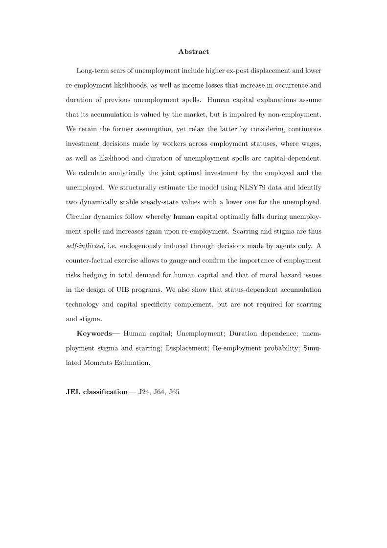
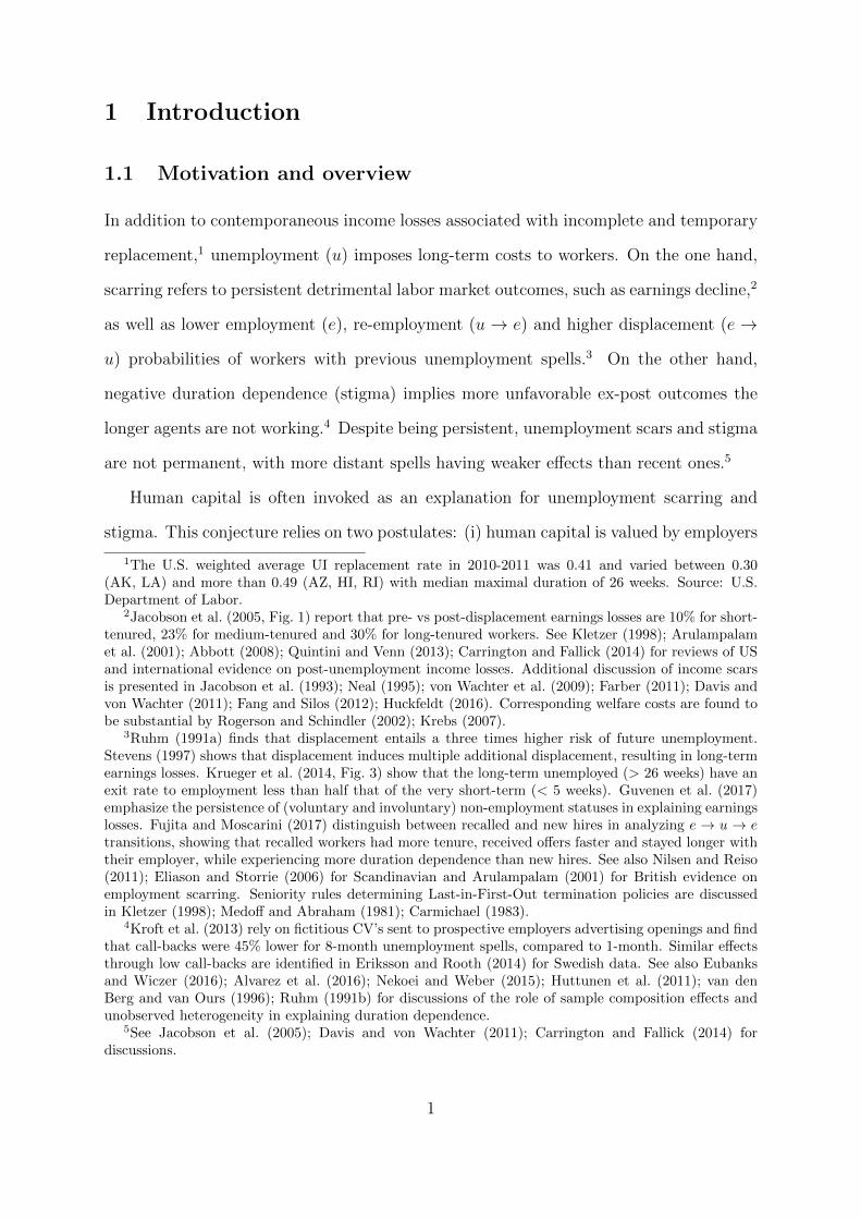
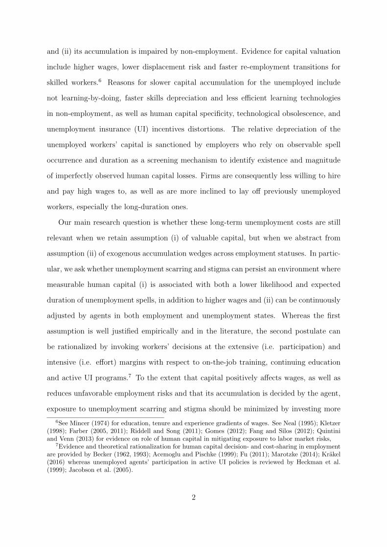
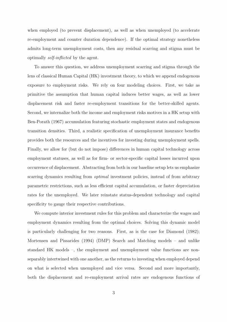
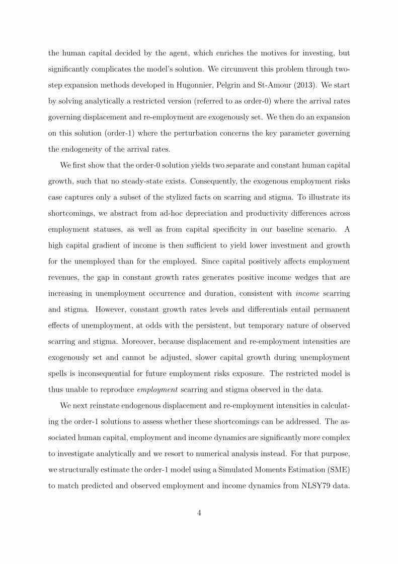
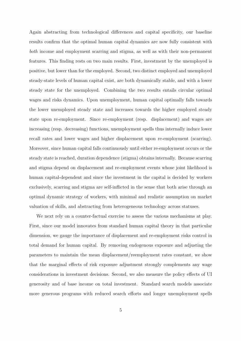
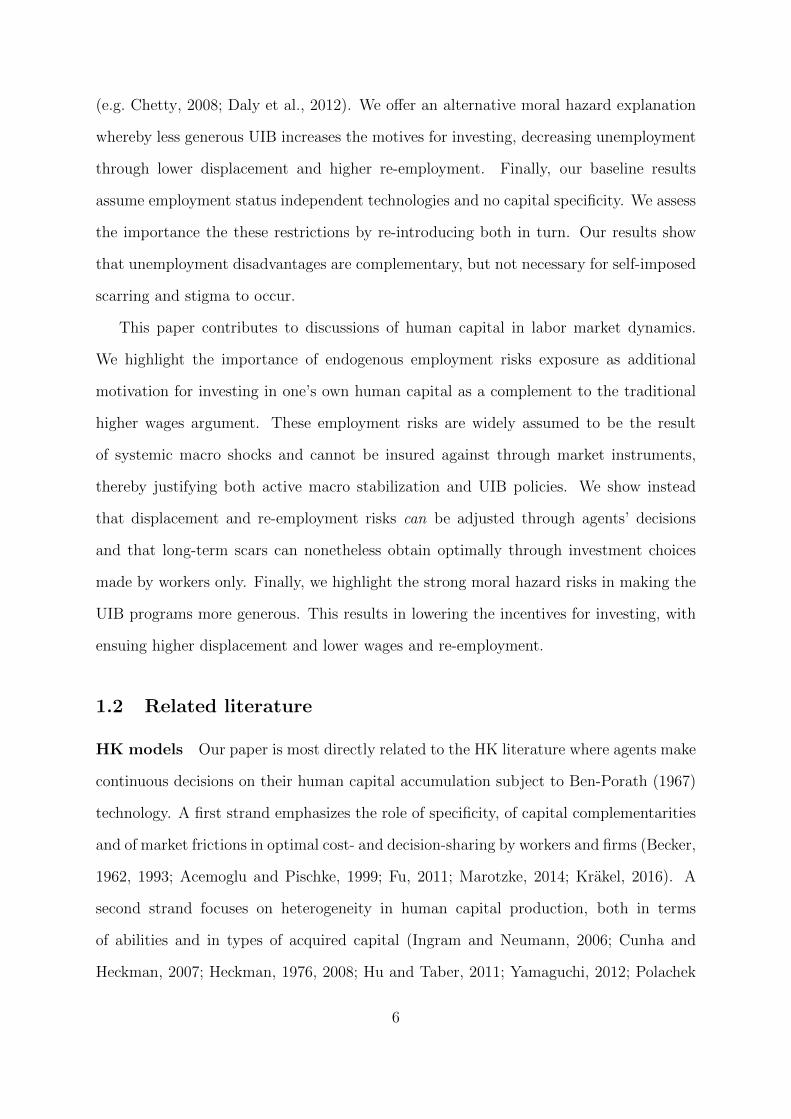
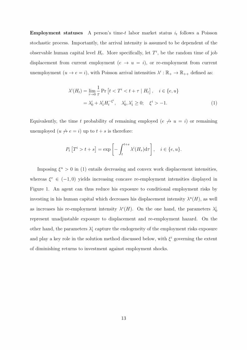
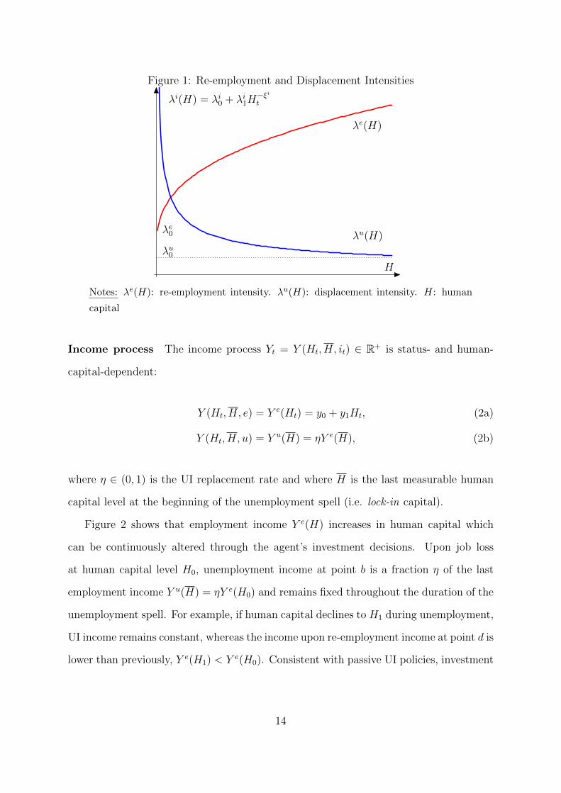
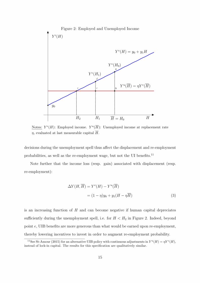
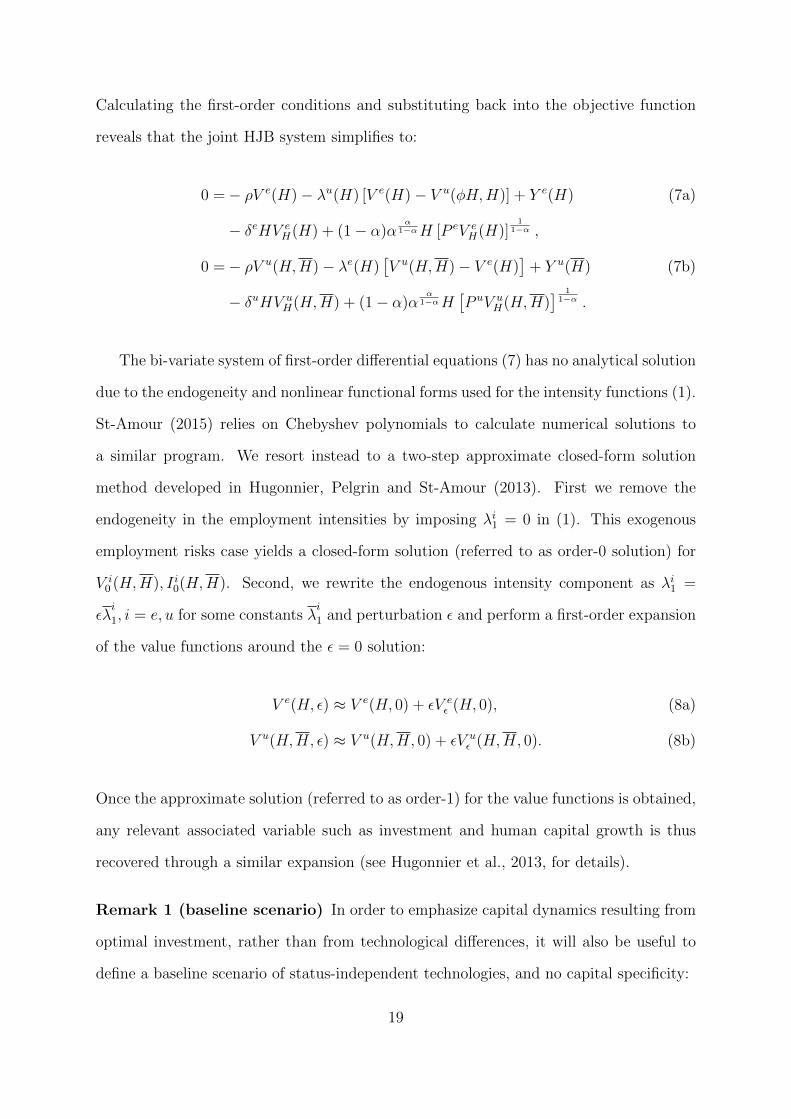

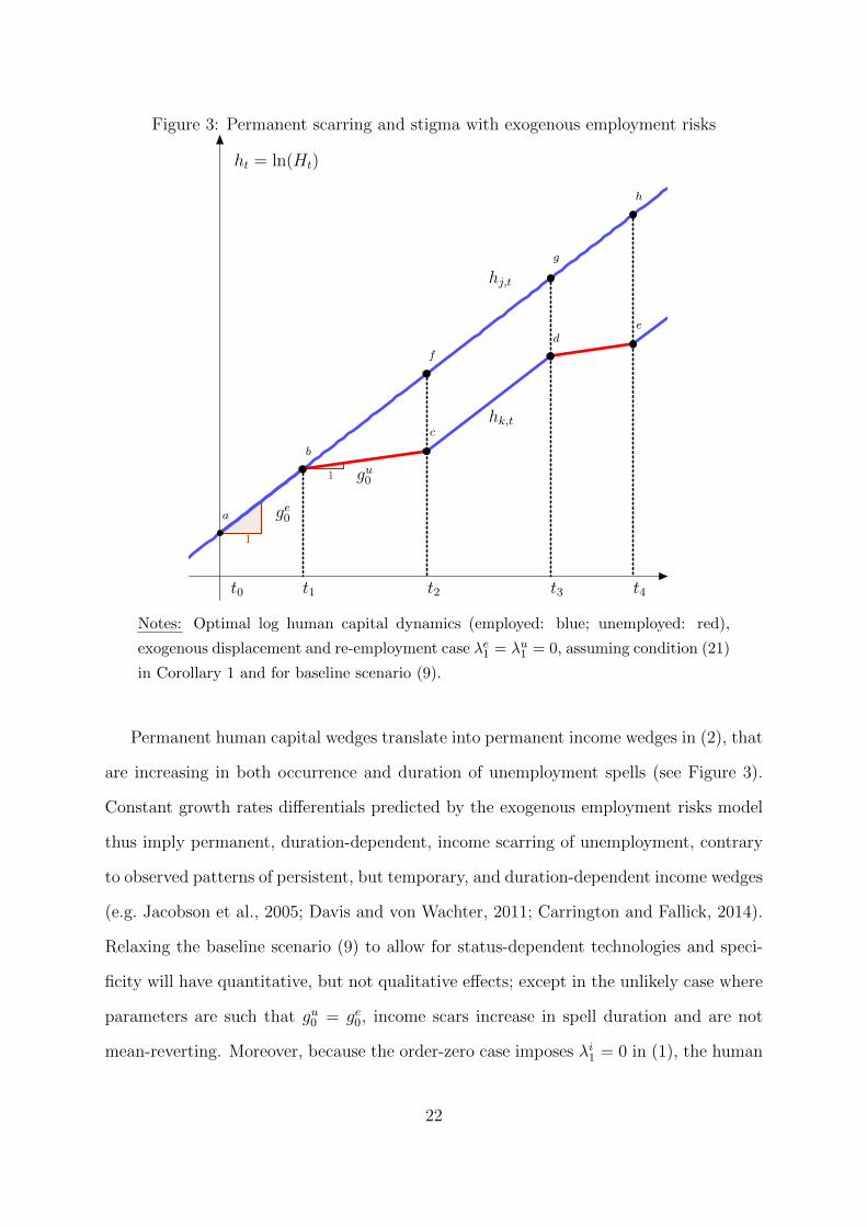
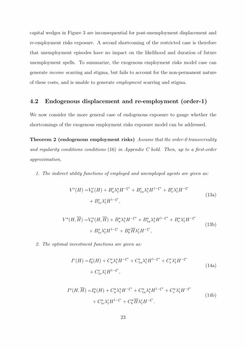
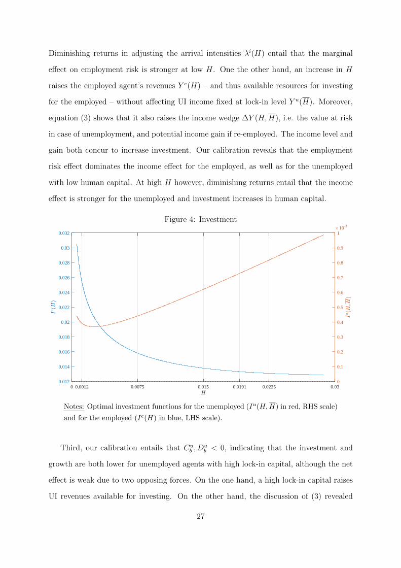
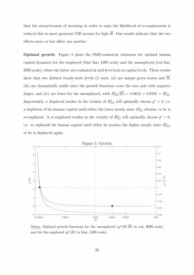
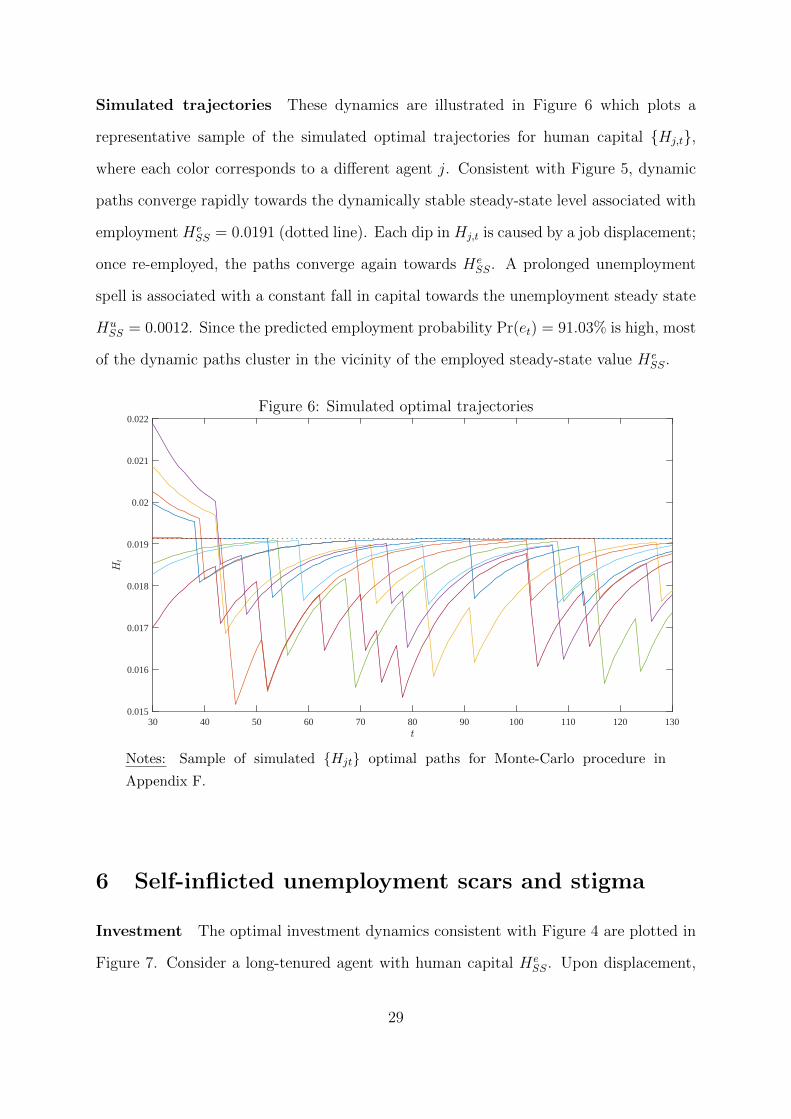
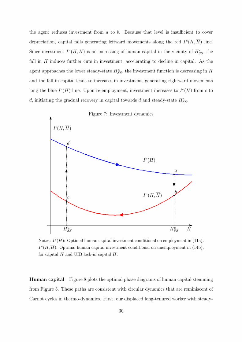
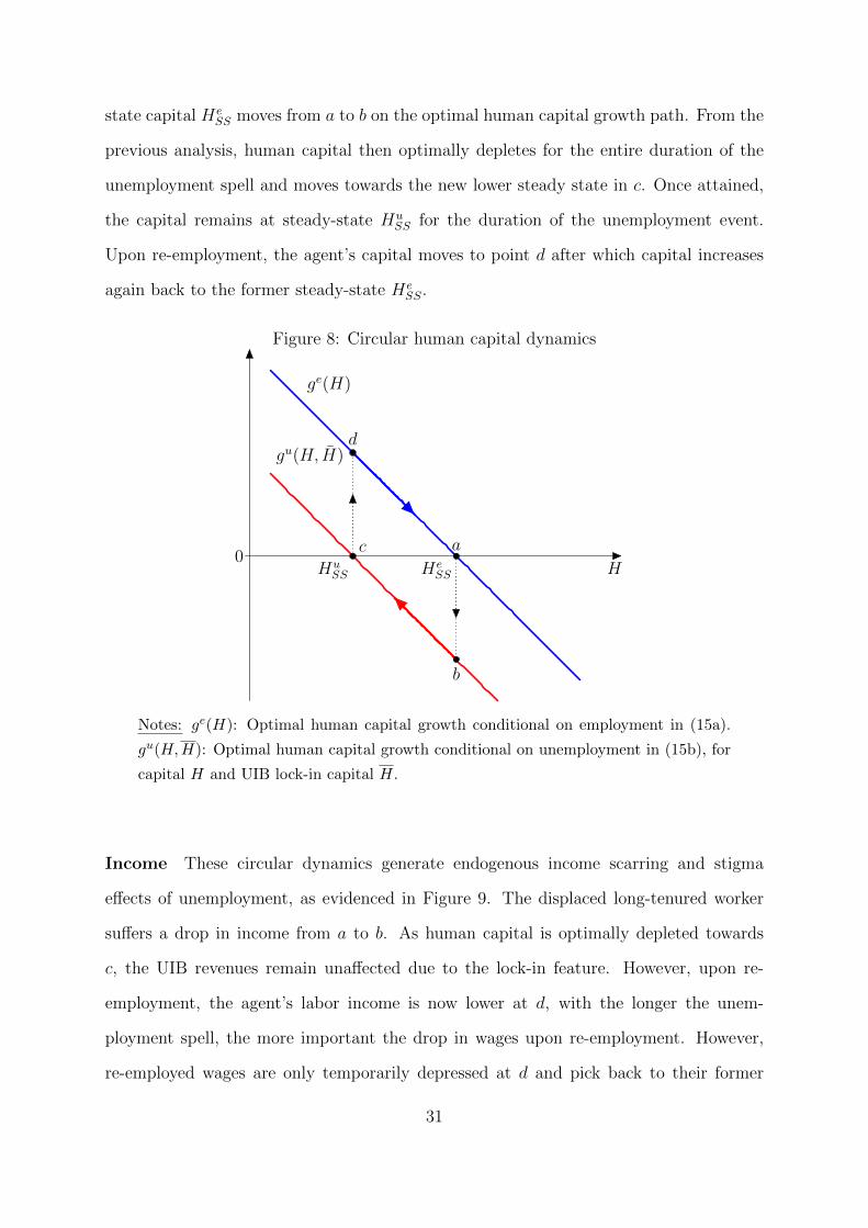
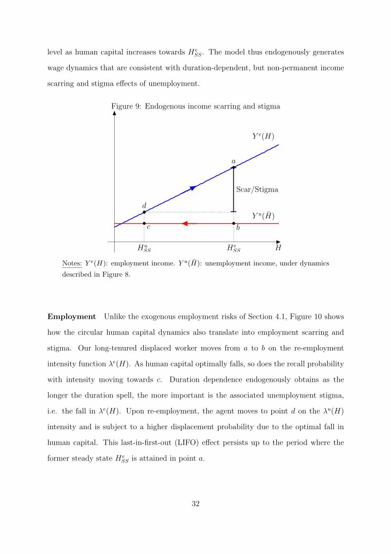
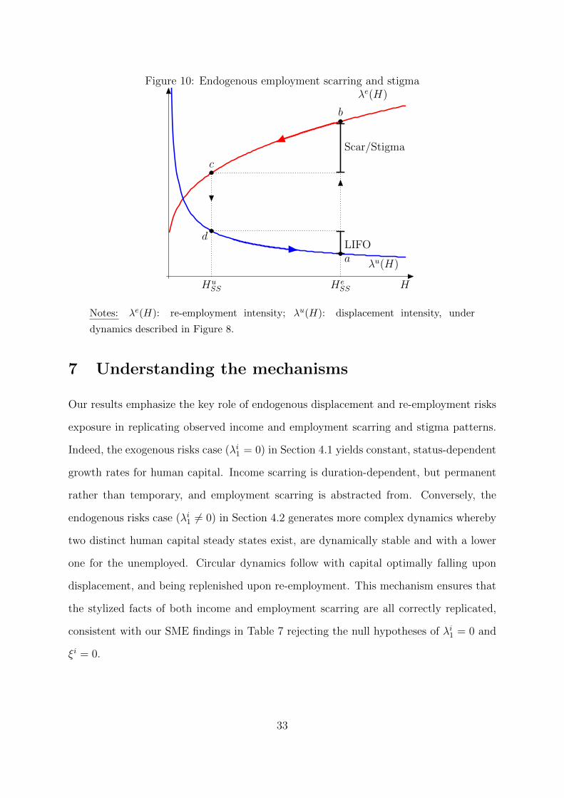
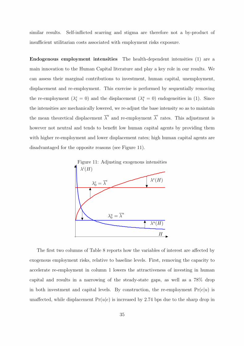
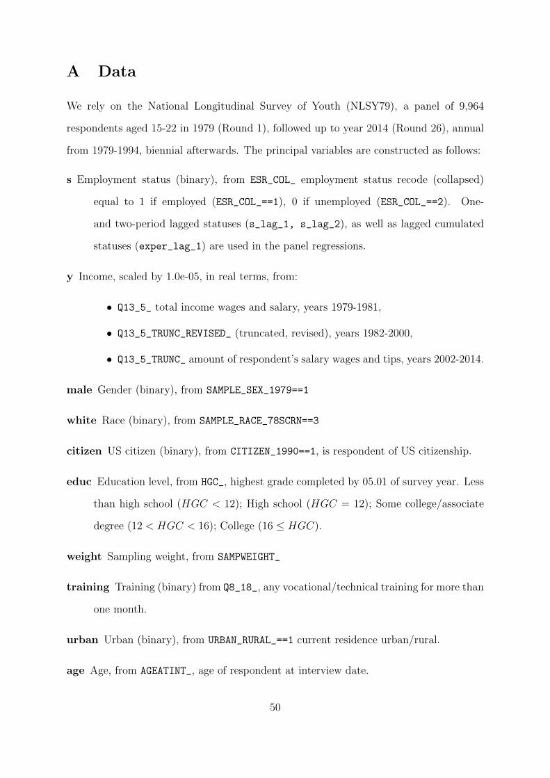
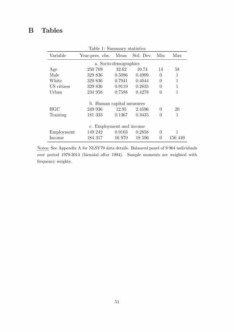
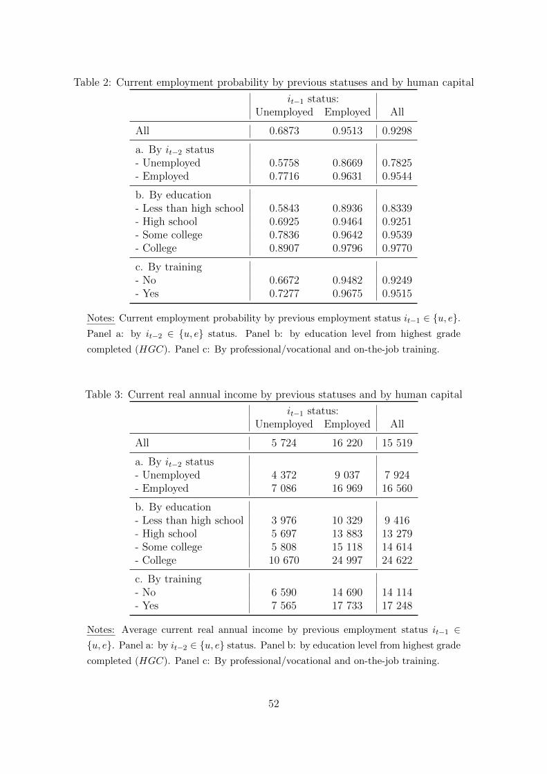
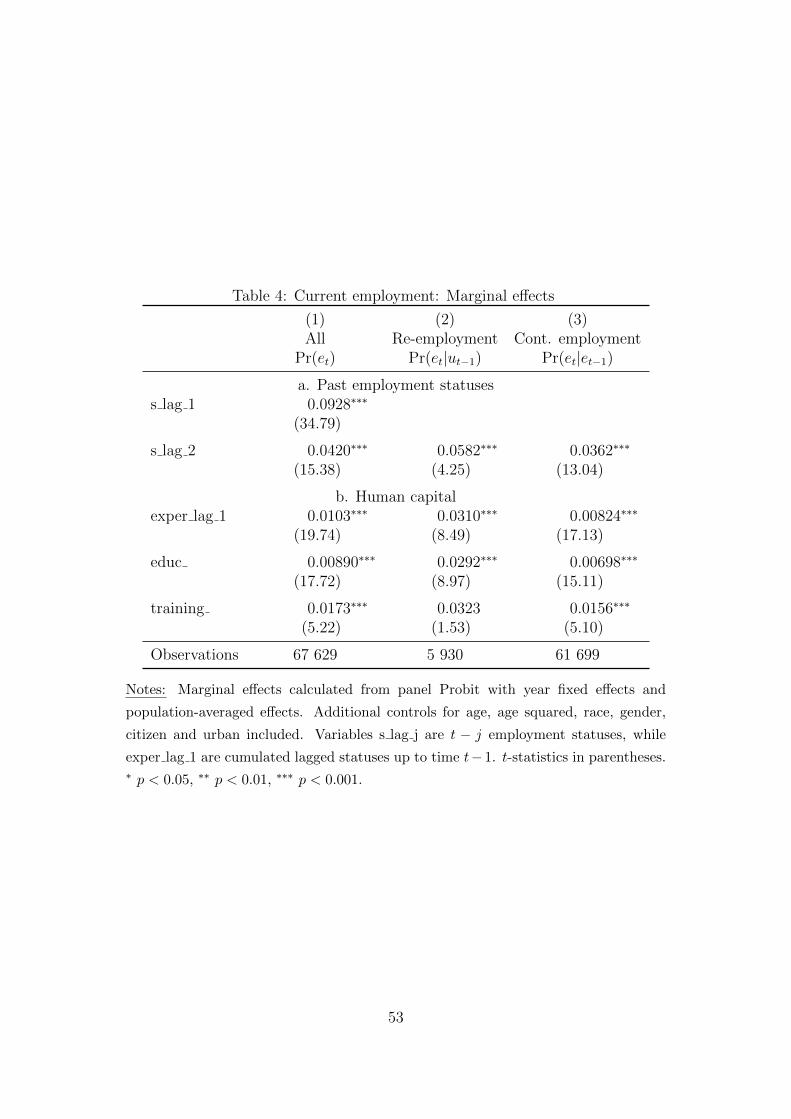
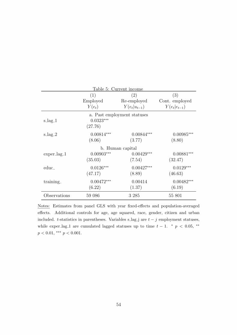
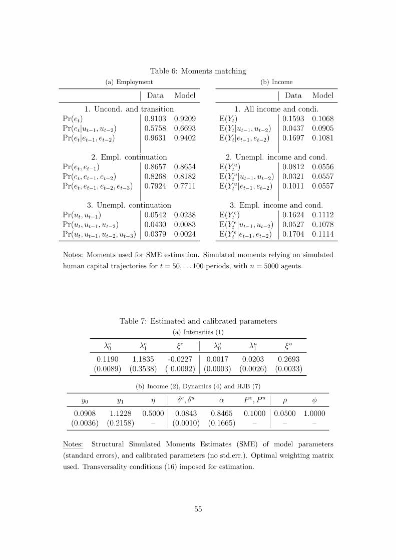
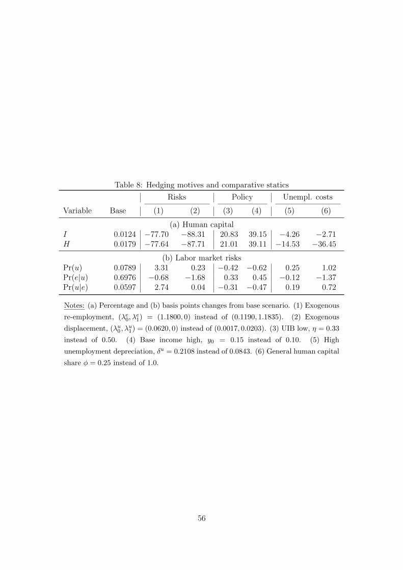
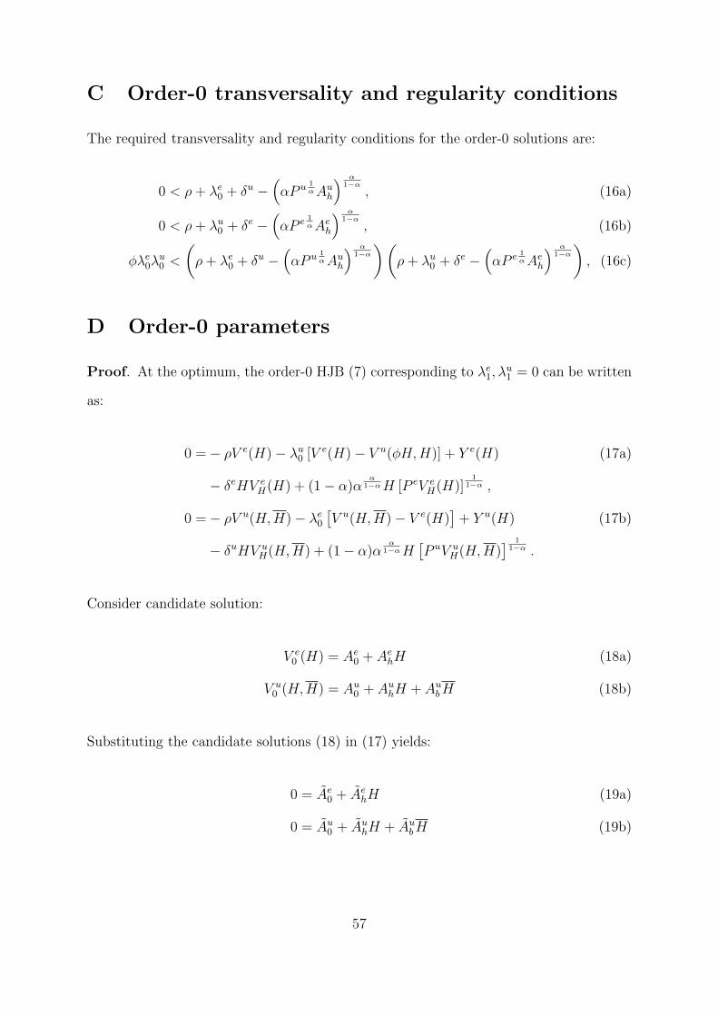
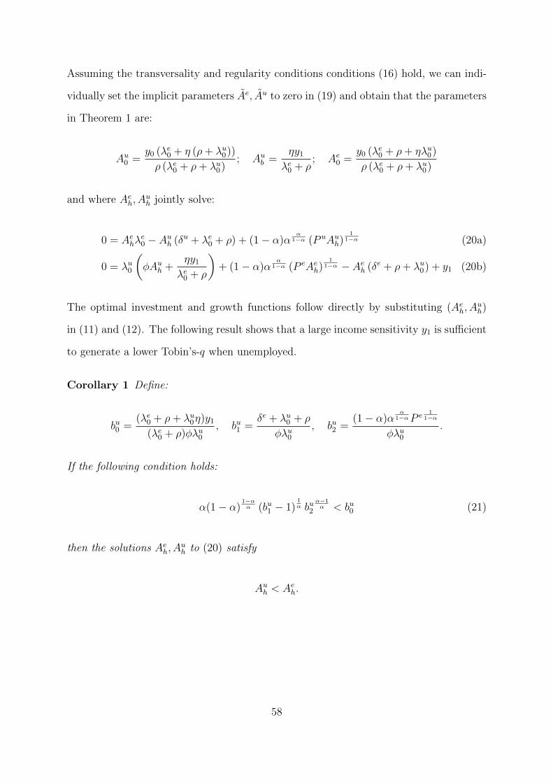
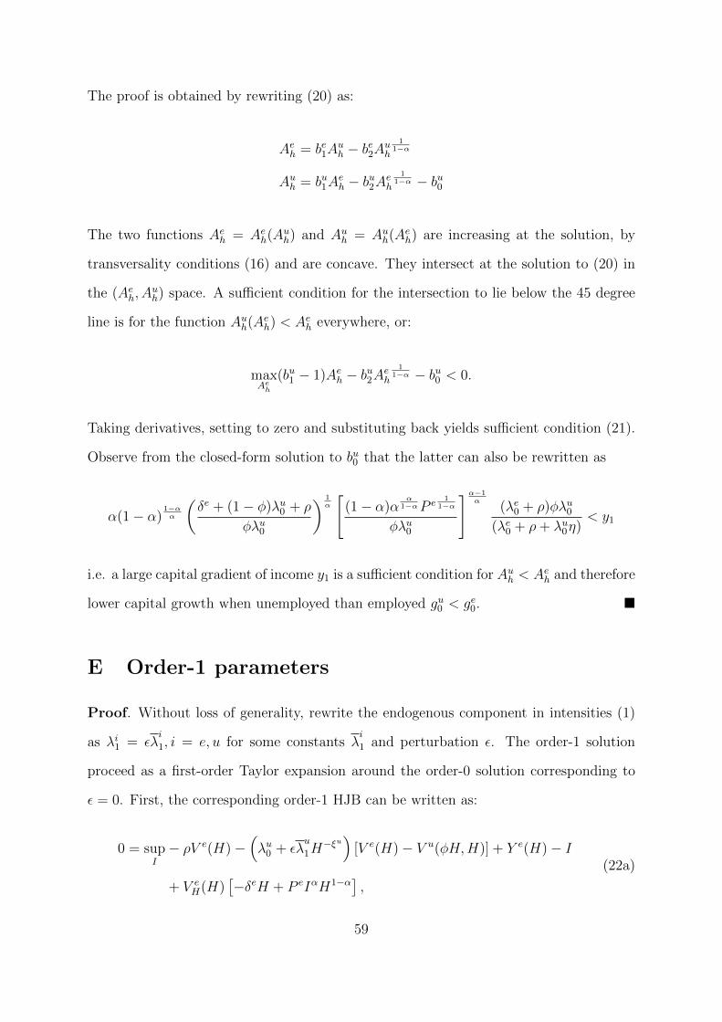
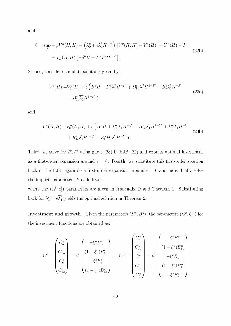
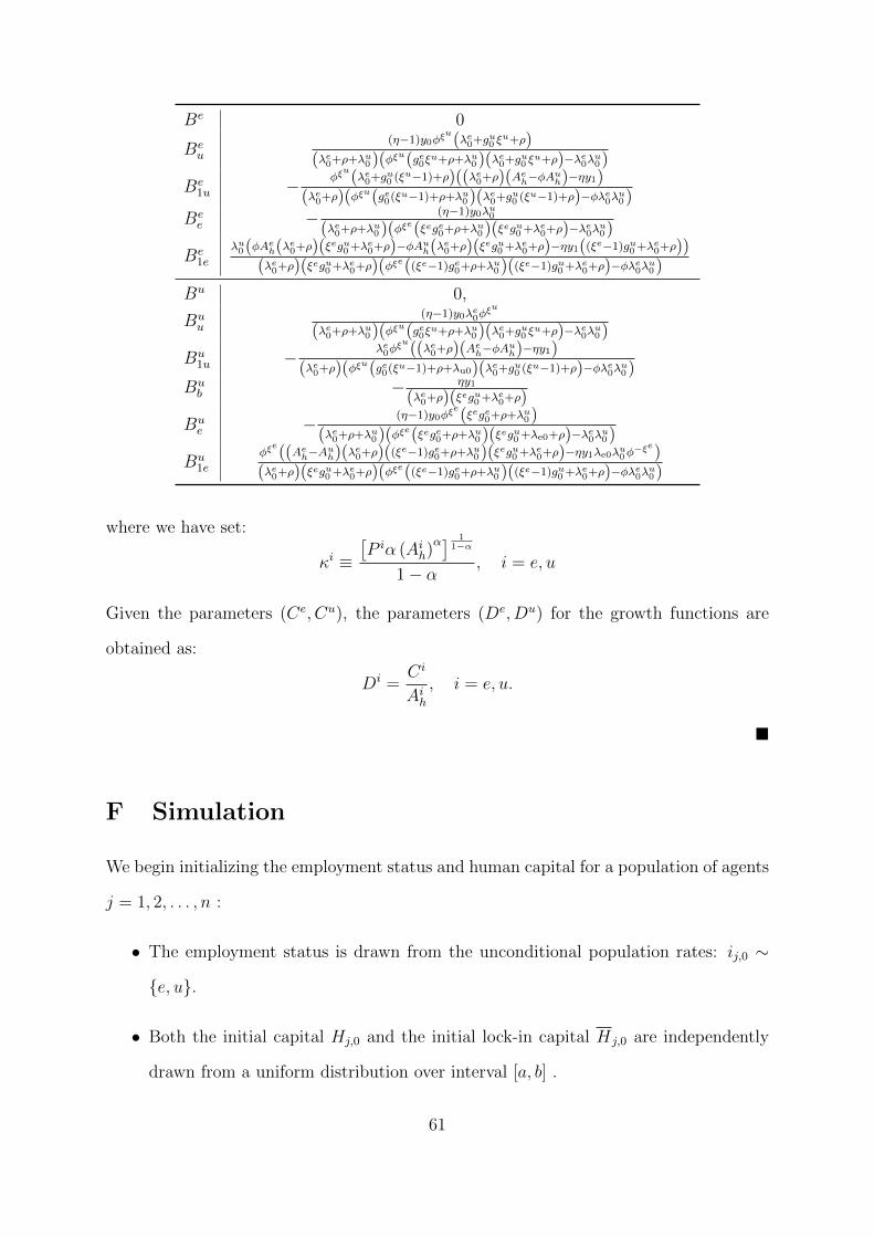
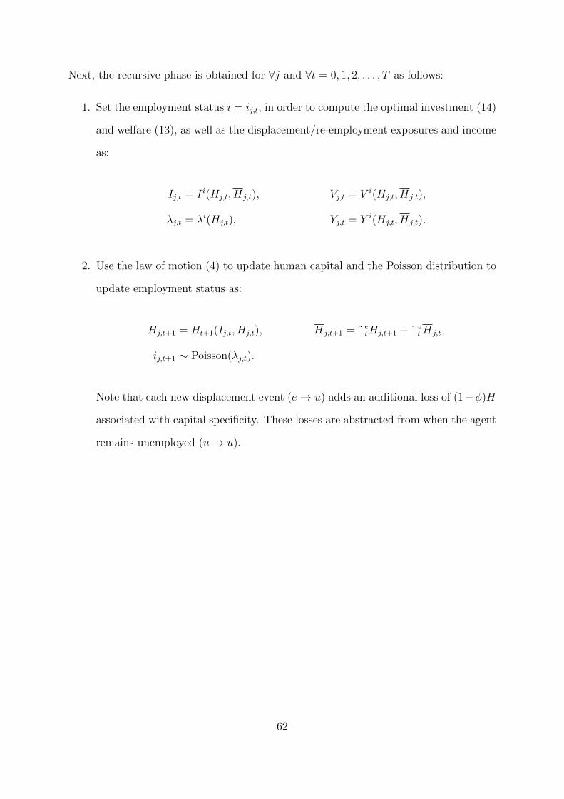


![Monitoring Managers: Does it Matter? [EBRD - Publications] · Monitoring managers: does it matter?* Francesca Cornelli, Zbigniew Kominek and Alexander Ljungqvist Summary We test under](https://static.documents.pub/doc/80x56/5f6cc61f49fb787f9d625a5a/monitoring-managers-does-it-matter-ebrd-publications-monitoring-managers.jpg)


