Self-organization and missing values in SOM and GTM

T. Vatanen a,b,n, M. Osmala a, T. Raiko a, K. Lagus a, M. Sysi-Aho c, M. Orešič d,T. Honkela e, H. Lähdesmäki a

a Aalto University School of Science, Department of Information and Computer Science, P.O. Box 15400, FI-00076 Aalto, Espoo, Finlandb The Broad Institute of MIT and Harvard, 7 Cambridge Center, Cambridge, MA 02142, USAc VTT Technical Research Centre of Finland, Espoo FI-02044, Finlandd Steno Diabetes Center, 2820 Gentofte, Denmarke University of Helsinki, Department of modern languages, P.O. Box 24, FI-00014 Helsinki, Finland

a r t i c l e i n f o

Article history:Received 12 April 2013Received in revised form18 January 2014Accepted 19 February 2014Available online 10 June 2014

Keywords:Self-organizing mapGenerative topographic mappingSelf-organizationMissing dataData visualization

a b s t r a c t

In this paper, we study fundamental properties of the Self-Organizing Map (SOM) and the GenerativeTopographic Mapping (GTM), ramifications of the initialization of the algorithms and properties of thealgorithms in the presence of missing data. We show that the commonly used principal componentanalysis (PCA) initialization of the GTM does not guarantee good learning results with high-dimensionaldata. Initializing the GTM with the SOM is shown to yield improvements in self-organization with threehigh-dimensional data sets: commonly used MNIST and ISOLET data sets and epigenomic ENCODE dataset. We also propose a revision of handling missing data to the batch SOM algorithm called theImputation SOM and show that the new algorithm is more robust in the presence of missing data.We benchmark the performance of the topographic mappings in the missing value imputation task andconclude that there are better methods for this particular task. Finally, we announce a revised version ofthe SOM Toolbox for Matlab with added GTM functionality.

& 2014 Elsevier B.V. All rights reserved.

1. Introduction

Topographic mappings, such as the Self-Organizing Map (SOM)[1,2] and the Generative Topographic Mapping (GTM) [3], areuseful tools in inspecting and visualizing high-dimensional data.The SOM was originally inspired by neuroscientific research oncortical organization, and the algorithm models the basic princi-ples of the organization process at a general level. The SOM hasbeen shown to serve its purpose well, especially when thefaithfulness (precision) of the mapping from a high-dimensionalspace is considered [4]. In practice, the SOM has proved to be arobust approach tested in thousands of different applications[5–7]. The GTM was inspired by the SOM algorithm, whileoperating in the probabilistic framework which provides well-founded regularization and model comparison [3]. In this paper,we show that both methods have their own strengths over theother and the methods may even benefit each other. We

investigate applicability of the methods in high-dimensional,real-life data sets and provide methodological improvements inthe presence of missing data.

Visualization of biological and life science data is an importanttask in the rapidly evolving field of bioinformatics. New kinds ofmeasurement techniques and visualization methods appear at aconstant pace (see, e.g., www.vizbi.org), but many practitionersstill turn to rudimentary methods, such as hierarchical cluster-ing and heatmaps. Recently, [8,9] have used the SOM in order tocluster genome segmentation regions based on different assaysignal characteristics gathered in the Encyclopedia of DNAElements (ENCODE) project. The SOM is particularly well suitedfor many visualization tasks on biological data because of itscomputational simplicity and relatively loose prior assumptionson the data. As we will show, the Gaussian noise model assumedin the GTM is a critical constraint for many high dimensional datasets. Furthermore, a SOM-type mapping has also been adapted toarbitrary data for which the mutual pairwise distances are defined[10] allowing one to compute SOMs only based on pairwisedistance matrices. A comprehensive review of visualization methodsfor large data sets can be found, e.g., in [11].

Missing data are a common problem in many data-dependentfields ranging from social sciences to economics and from politicalresearch to entertainment industry. In fields where conductingsurveys or polls is commonplace, missing data occurs, for instance,

Contents lists available at ScienceDirect

journal homepage: www.elsevier.com/locate/neucom

Neurocomputing

http://dx.doi.org/10.1016/j.neucom.2014.02.0610925-2312/& 2014 Elsevier B.V. All rights reserved.

n Corresponding author at: Aalto University School of Science, Department ofInformation and Computer Science, P.O. Box 15400, FI-00076 Aalto, Espoo, Finland.

E-mail addresses: tommi.vatanen@aalto.fi (T. Vatanen),maria.osmala@aalto.fi (M. Osmala), tapani.raiko@aalto.fi (T. Raiko),krista.lagus@aalto.fi (K. Lagus), marko.sysi-aho@vtt.fi (M. Sysi-Aho),matej.oresic@gmail.com (M. Orešič), timo.honkela@aalto.fi (T. Honkela),harri.lahdesmaki@aalto.fi (H. Lähdesmäki).

Neurocomputing 147 (2015) 60–70

when people refuse to answer to specific questions or some peoplecannot be contacted. In the movie business, predicting customerpreferences is literally a million dollar quest. The Netflix Prize(see, e.g., [12]) was an open competition to devise the bestrecommendation system to predict user ratings for films basedon previous ratings. In the second part of this paper, we present arevision to the batch SOM algorithm, called the Imputation SOM,which is shown to improve the behavior of the SOM algorithm inthe presence of missing data.

This paper is organized as follows. Sections 2 and 3 introducethe SOM and the GTM models, respectively. In Section 4, theproperties of the models are compared in terms of self-organization and convergence. We show that using the SOM forinitializing the GTM may improve the learning results in somecases. Section 5 explains the treatment of missing values inthe GTM and adapts the same principled way into the SOM.Performance of the algorithms is compared in a missing valueimputation task. Finally, the results and possible future work arediscussed in Section 6.

In all the experiments, the SOM Toolbox [13] and Netlab [14]software packages are used. The GTM scripts in Netlab are revisedto handle data with missing values and a sequential trainingalgorithm is contributed. Also, an issue of small probabilities beingrounded to zero due to insufficient floating point precision wassolved. Finally, we announce a revised version of the SOM Toolboxwhich incorporates GTM functionality. An up-to-date version ofthe SOM Toolbox is available at

http://research.ics.aalto.fi/software/somtoolbox

2. Self-organizing map

The self-organizing map (SOM) [2] discovers some underlyingstructure in data using K map units, prototypes or referencevectors fmig. For the prototypes, explicit neighborhood relationshave been defined. The classical sequential SOM algorithm pro-ceeds by processing one data point xðtÞ at a time. Euclidean, or anyother suitable distance measure is used to find the best-matchingunit given by mcðxðtÞÞ ¼ arg mini‖xðtÞ�mi‖. The reference vectorsare then updated using the update rule miðtþ1Þ ¼miðtÞþhciðtÞðxðtÞ�miðtÞÞ, where an explicit neighborhood functionhci ¼ αðtÞ � expf�‖rc�ri‖2=2σ2ðtÞg is used in order to obtain topo-logical mapping. In the neighborhood function, ‖rc�ri‖ is thedistance between the best-matching unit rc and unit i in the array,0oαðtÞo1 is scalar-valued learning-rate factor and σðtÞ is thewidth of the neighborhood kernel.

2.1. Batch SOM

In the Batch SOM, the reference vectors are updated using alldata (or a mini-batch, a part of the data) at once and weightedaccordingly. The batch update rule is

mi ¼∑nhnixn

∑jhni

; ð1Þ

where the index n runs over the data vectors whose best-matchingunits satisfy hni40, that is, all data points up to the range of theneighborhood function are taken into account.

2.2. Quality and size of the SOM

Selecting the size of the array of map units in the SOM is asubtle task. Previously many solutions, such as hierarchical [15]and growing maps [16,17], have been proposed to tackle this issue.The question of the size can be approached from the point of view

of different quality measures. Two most commonly used errormeasures are the quantization error and the topological error [2].The former measures the mean of the reconstruction errors‖x�mc‖ when each data point used in learning is replaced by itsbest-matching unit. The latter measures the proportion of datapoints for which the two nearest map units are not neighborsin the array topology. As the number of map units increases,quantization error decreases and topological error tends toincrease. Hence, there is no straightforward way of choosing thenumber of map units based on the measures above. Topographicpreservation has been studied in detail, e.g., in [18,4,19]. In thiswork, we use an error measure proposed in [20]. This combinederror is a sum of the quantization error and the distance from thebest-matching unit to the second-best-matching unit of each datavector along the shortest path following the neighborhood rela-tions. More formally, using the notation in [20], the distancemetric used is given by

dðxÞ ¼ ‖x�mc‖þ ∑Kc0 ;i �1

k ¼ 0‖mIiðkÞ �mIiðkþ1Þ‖; ð2Þ

where the first term is the quantization error and the second termcomputes the distance between the BMU and the second-best-matching unit along the map grid. Given a training data fxngNn ¼ 1,combined error is given by

EC ¼ ∑N

n ¼ 1dðxnÞ; ð3Þ

where n runs over all the data vectors. We have added this featurein the SOM Toolbox som_quality function and demonstrate itsuse in the experiments.

3. Generative topographic mapping

The Generative Topographic Mapping (GTM) [3,21] is a non-linear latent variable model which was proposed as a probabilisticalternative to the SOM. Loosely speaking, it extends the SOM in asimilar manner as Gaussian mixture model extends k-meansclustering. This is achieved by working in a probabilistic frame-work where data vectors have posterior probabilities given a mapunit. Hence, instead of possessing only one best-matching unit,each data vector contributes to many reference vectors directly.

The GTM can be seen consisting of three parts: (1) discrete setof points in usually one or two-dimensional latent space, (2) non-linear mapping, usually radial basis function (RBF) network,between the latent space and the data space, and (3) a Gaussiannoise model in the data space such that the resulting model is aconstrained mixture of Gaussians. In this paper, latent points fuig,which are arranged in a regular grid, are mapped to the data spaceusing M fixed radial basis functions ϕðuiÞ ¼ fϕjðuiÞg, whereϕjðuiÞ ¼ expf�‖cj�ui‖=σ2g, σ is the width parameter of the RBFs,fcjg are the RBF centers and j¼1,…,M. The number of RBFs, M, is afree parameter which has to be chosen by the experimenter. Theradius of the RBFs is chosen according to σ ¼ dmax=

ffiffiffiffiffiM

p, where dmax

is the maximum distance between two RBF centers (this is atextbook choice for RBF networks; see, e.g. [22]). The nodelocations in latent space, ui, define a corresponding set of refer-ence vectors mi ¼WϕðuiÞ in the data space, where W is a weightmatrix defining the mapping from the latent space to the dataspace. In this work, each reference vector mi serves as a center ofan isotropic Gaussian distribution in the data space

pðxjmiÞ ¼β2π

� �D=2

exp �β2‖mi�x‖2

� �; ð4Þ

where β is the precision or inverse variance. The Gaussiandistribution above also represents a noise model accounting for

T. Vatanen et al. / Neurocomputing 147 (2015) 60–70 61

the fact that the data will not be confined precisely to the lower-dimensional manifold in the data space. More general noisemodels have been proposed [21].

The probability density function of the GTM is obtained bysumming over the Gaussian components yielding

pðxjW ;βÞ ¼ ∑K

i ¼ 1PðmiÞpðxjmiÞ ¼ ∑

K

i ¼ 1

1K

β2π

� �D=2

exp �β2‖mi�x‖2

� �;

ð5Þwhere K is the total number grid points in the latent space, or mapunits in the SOM terminology, and the prior probabilities PðmiÞ aregiven equal probabilities 1/K.

The GTM represents a parametric probability density model,with parameters W and β, and it can be fitted to a data set fxng bymaximum likelihood. The log-likelihood function of the GTM isgiven by

log ðLðW ;βÞÞ ¼ ∑N

n ¼ 1log pðxnjW ;βÞ; ð6Þ

where pðxnjW ;βÞ is given by (5) and independent, identicallydistributed (iid) data is assumed. We solved numerical issues inNetlab GTM implementation [14] by computing log-likelihood asfollows:

log ðLðW ;βÞÞ ¼ logpðxÞmaxþ log ∑N

n ¼ 1expðlogpðxnÞ� logpðxÞmaxÞ

� �;

ð7Þwhere pðxÞmax ¼maxn pðxnjW ;βÞ. In the experiments, negativelog-likelihood-per-sample, given by

EGTM ¼ � log ðLðW ;βÞÞ=N; ð8Þis used as a training error. The error can be minimized using theEM algorithm or alternatively any standard non-linear optimiza-tion technique.

4. Self-organization and convergence

Both the GTM and the batch SOM require careful initializationin order to self-organize [23,24]. For both algorithms, the commonchoice is to initialize according to the plane spanned by the twomain principal components of the data. In the batch SOM, theneighborhood is annealed during the learning which decreases therigidness of the map. The most important advantages of the batchSOM when compared to the classical sequential SOM are quickconvergence and computational simplicity [24].

As we will show, initializing the GTM using PCA does notalways lead to appropriate results. Instead, we propose using thebatch SOM for initializing the GTM. In the SOM initialization, usingfew epochs of ’rough training’ with wide neighborhood willsuffice. Next, W can be determined by minimizing the errorfunction:

Einit ¼12∑i‖WϕðuiÞ�mSOM

i ‖; ð9Þ

where mSOMi are the reference vectors of the initializing SOM. The

initializing SOM can, in turn, be initialized using PCA, which makesthe whole process deterministic.

Differences between the SOM and the GTM, and efficacy of theSOM initialization are demonstrated using several high-dimensional data sets. These data sets were chosen to demon-strate cases where the different initialization methods make adifference to the resulting mapping.

In the first example, we use the ISOLET data set from the UCImachine learning repository [25]. The data contains 7797 spokensamples of the letters of the alphabet. The 617 features are

described in [26] and include, e.g., spectral coefficients, contourfeatures and sonorant features. The data was normalized to havezero mean and unit variance. The class labels, i.e., the letteridentifiers, were not used in training of the maps.

The appropriate model complexity for the GTM, i.e, the numberof RBFs and latent points, can be chosen, e.g., by cross-validatingthe negative log-likelihood. Using cross-validation for the ISOLETdata, a suitable number of RBFs was found to be 400 (20�20) anda suitable number of map units 4004 (77�52). We used the samedata to demonstrate effects of the SOM initialization already in[27]. However, after improving the Netlab GTM functions to tacklenumerical issues (see Eq. (7)), the results obtained are significantlydifferent.

Fig. 1 shows two GTM visualization of the ISOLET data. In Fig. 1(a), PCA initialization was used, whereas in Fig. 1(b) the GTM wasinitialized using the SOM. The map initialized using the SOM hasbetter cluster structure where most of the letters form distinctclusters. Furthermore, similar sounding letters are mapped closeto each other. On the left side of the map, the data is moreambiguous and different letters, such as B, D, E, P, and V, are mixedtogether.

The GTM in Fig. 1(a), initialized with PCA, also has some clusterstructure, but most of the letters are spread over wider areacompared to the Fig. 1(b). However, when comparing to the resultsin [27], where the GTM with PCA initialization was not able tolearn any interesting structure in the ISOLET data, there is asignificant improvement caused by our implementations of

Fig. 1. A GTM of the ISOLET data with 4004 (77�52) map units and 400 (20�20)RBFs initialized using (a) PCA and (b) the SOM. Bootstrapped mean training error,EGTM (8), is (a) 563.1 and (b) 545.8. (a) PCA initialization. (b) SOM initialization.

T. Vatanen et al. / Neurocomputing 147 (2015) 60–7062

standard numerical precision tricks in the GTM algorithms. Evolu-tion of bootstrapped training errors for the both GTMs is shown inFig. 2(a). The GTM with the SOM initialization converges to lowertraining error, EGTM (8). Mean bootstrap estimates (standarddeviations in parentheses) for final training errors are 563.1 (1.4)for PCA initialization and 545.8 (1.3) for SOM initialization.

The MNIST data set (see http://yann.lecun.com/exdb/mnist/)contains 60 000 training samples and 10 000 test instances ofhandwritten digits. We use this separation in order to assessgeneralization of the GTM. Each feature in the data set is a grayscale value of a pixel, between zero and one. Fig. 3 shows theMNIST test instances mapped on GTMs trained using the MNISTtraining data with (a) PCA and (b) the SOM initialization. The mapswere trained using the sequential training algorithm, whichspeeds up the convergence [21]. When mini-batch size of 10 000was used, only five epochs of training was needed for sufficientconvergence. The evolution of bootstrapped training errors isshown in Fig. 2(b). When comparing the resulting GTMs, the sameobservations can be made as for the ISOLET data. Both GTMsshow some cluster structure, but this structure is clearer in theGTM initialized using the SOM. Bootstrapped mean estimates andstandard deviations in parenthesis for test error (8) evaluatedusing test data are �255.0 (1.4) and �249.7 (1.3) for SOM and PCAinitialization, respectively (standard deviations in parentheses).

For third high-dimensional data demonstration we use epige-nomic measurements obtained by the ENCODE consortium [8].The ENCODE data was recently used in [9] in order to train a largeSOM to identify complex relationships in epigenomic measure-ments and other genomic data. The authors computed the RPKM(Reads Per Kilobase per Million reads) values from the signal of 72measurements over six cell lines on 1.5 million genome segments.The resulting data matrix was used to train a SOM of size 30 times45 units. The clusters, revealed by SOM, are associated withgeneral and cell type-specific gene activity, and regulatory regionssuch as promoters and enhancers. The authors show that thedistinct combination of epigenetic signals associated to a particu-lar cluster can be used to find new genomic loci of that particulartype. Here we use ChIP-seq read density profiles of only fivedifferent histone modifications (H3K4me1, H3K4me3, H3K79me2and H3K9ac and H3K27me3) in human chronic myelogenousleukemia (K562) cell line. The goal is to investigate whetherenhancers, promoters and random background regions form dis-tinct clusters in GTM. The 1000 most significant p300 binding sitesdistal to any transcription start site (TSS), and the 1000 mostsignificant DNase I hypersensitivity sites (DHSs) overlapping anyTSS were used as a set of true enhancers and active promoters,respectively. In addition, histone modification signals at 1000

random locations were used as background samples. The randomlocations were sampled from genomic regions having the totalread density signal greater or equal to 10, hence avoiding samplingregions with zero signal. The read density profiles at these siteswere extracted using a 5000 base pair window centered on theregion of interest, and further averaged over every fifth nucleotide.Finally the five histone modification signal profiles were

0 5 10 15 20540

560

580

600

620

640

660

680

700

epoch

train

ing

erro

r

PCA initSOM init

1 2 3 4 5

−260

−250

−240

−230

−220

−210

−200

epoch

train

ing

erro

r

PCA initSOM init

Fig. 2. Bootstrapped means and ranges of training error (8) evolution of GTMs trained using (a) the ISOLET data and (b) the MNIST data. For the MNIST data, sequentialtraining with mini-batch size of 10 000 is used and only five training epochs is needed. In both cases, the GTMs with the SOM initialization converge to smaller training error.(a) ISOLET data. (b) MNIST data.

Fig. 3. The mapping of MNIST validation data on GTMs trained using MNISTtraining data and initialized using (a) PCA and (b) the SOM. Bootstrapped mean testerror, EGTM (8), is (a) �249.7 and (b) �255.0. (a) PCA initialization. (b) SOMinitialization.

T. Vatanen et al. / Neurocomputing 147 (2015) 60–70 63

concatenated to form 5000 dimensional vectors. The data wasnormalized by subtracting the mean and dividing by the standarddeviation.

Fig. 4 shows GTMs trained using the ENCODE data. Thedifference between PCA and the SOM initializations is obvious,even though the difference of the bootstrapped final trainingerrors, EGTM (8) (standard deviation in parentheses), is onlyless than 2%, 4662.3 (53.0) vs. 4463.5 (51.1) for PCA and SOMinitialization, respectively. In Fig. 4(b), different genomic regions,promoters (green), enhancers (red) and background sequences(blue) are clustered in distinct regions of the map. The mixing ofenhancers, promoters and random background clusters mayreflect the fact that not all TSS overlapping DHS or TSS-distalp300-binding sites necessarily are active promoters and enhancers,respectively, and hence do not show promoter or enhancer-specificepigenetic marks. The random background samples may also containactive promoters and enhancers.

5. Missing values

In this section, we discuss the behavior of topographic map-pings in the presence of missing values. We start by showing howmissing values are treated in the GTM and develop the same ideafor the SOM. The section is concluded by an experimental study

where even low-dimensional data sets reveal differences betweenthe studied algorithms.

In all what follows, missing-at-random (MAR) data is assumed.This means that the probability of missingness is independent ofmissing values given the observed data. Even though this assump-tion can be questioned in many real-life scenarios, this is usually areasonable assumption given that only a small proportion of thedata is missing.

5.1. GTM and missing values

The GTM offers a robust framework for dealing with missingvalues, noted already in [3]. As with any method operating in theprobabilistic framework, missing values can be handled by inte-grating them out. If the missing values are MAR, this does notintroduce any bias. Hence, the maximum-likelihood estimation ofthe model parameters θ reduces to maximizing LðθjXobsÞ ¼pðXobsjθÞ, where Xobs denotes the observed data. For the GTM,the likelihood function is given by

LðW ;βjXobsÞ ¼ pðXobsjW ;βÞ ¼Z

pðXobsjXmis;W ;βÞ dXmis; ð10Þ

where Xmis denotes the missing or unobserved data. This integra-tion can be performed analytically for the standard GTM with anisotropic noise model.

The handling of missing data can be incorporated in the EMalgorithm in a straightforward manner. In the E-step, whereposterior probabilities of data vectors given the map units arecalculated, missing values are simply omitted. That is, the distancebetween the map units and a data vector with missing value(s) isevaluated only in the dimensions observed for the correspondingdata vector. In the M-step, the expected values of the missing dataand other sufficient statistics are used. The details of learningthe GTM with missing values using the EM algorithm can be foundin [28].

After the training, there are at least two possibilities to performimputation in the GTM. One may use the expected valuesEðXmisjXobs;W ;βÞ or impute using the maximum-a-posteriori(MAP) estimates pMAPðXmisjXobs;W ;βÞ which takes the missingvalues from the most similar map unit. Additionally, multipleimputations can be conducted by sampling the posterior distribu-tion pðXmisjXobs;W ;βÞ.

5.2. SOM and missing values

The SOM has been used for missing value imputation withmany kinds of data, such as survey data [29,30], socioeconomicdata [31], industrial data [32,33] and climate data [34]. In most ofthe SOM literature, the missing values are treated as was proposedin [31]. The best-matching units for the data vectors with missingvalues are computed by omitting the missing values. This isconsistent with the procedure in the probabilistic setting. Themissing values are ignored also while updating the referencevectors. This approach is implemented in the widely used SOMToolbox [13]. After the training, missing values can be filledaccording to the best-matching units of the corresponding datavectors.

5.2.1. Imputation SOMA novel approach, named the Imputation SOM (impSOM), stems

from the way missing values are treated while using the GTM withan isotropic noise model (see above). The distances between datapoints and reference vectors are evaluated as described above,since this already corresponds to the statistical approach. Whileupdating the reference vectors, instead of ignoring the missing

Fig. 4. GTMs trained using epigenomic data measured by the ENCODE consortiumand initialized using (a) PCA and (b) the SOM. The promoter (green), enhancer (red)and background (blue) samples form semi-consistent clusters. Jitter is addedto make data points distinguishable. (a) PCA initialization. (b) SOM initialization.(For interpretation of the references to color in this figure caption, the reader isreferred to the web version of this paper.)

T. Vatanen et al. / Neurocomputing 147 (2015) 60–7064

data their expected values

x̂ni;mis ¼ E½xn;misjmi� ¼mi ð11Þare used. Above, expectation is used in an informal sense, since theSOM is not a statistical model. This results in an update rule,where the reference vectors are updated according to (1) such thatfor each unobserved component of xn the current value mi is used.Thus, the data with missing values contribute by restraining thereference vectors in the dimensions corresponding to the missingvalues.

5.3. Model selection

This section demonstrates several aspects of model selection.The wine data set from UCI machine learning repository is used. Itcontains 13 chemical properties of 178 wines that come from threedifferent wine regions. The data was normalized to have zeromean and unit variance and 5, 10, 30 and 50% of the values wererandomly removed for validation, resulting in missing-completely-at-random (MCAR) data set.

Selecting the number of map units for the SOM is a subtle task.If the purpose of using the SOM is missing value imputation, onedoes not have the RMS plot of Fig. 5(b) available without firstperforming some kind of validation. Moreover, traditional SOMerror measures, such as quantization and topological error, orcombined error (3) do not give any straightforward way ofdetermining a suitable map size. These difficulties in mind, thenumber of map units was deliberately increased above the numberof data points in both this and the next section. This allowedexperimenting the hypothesis that the excess map units

interpolate the data space allowing more precise imputation(see, e.g., [34,28]).

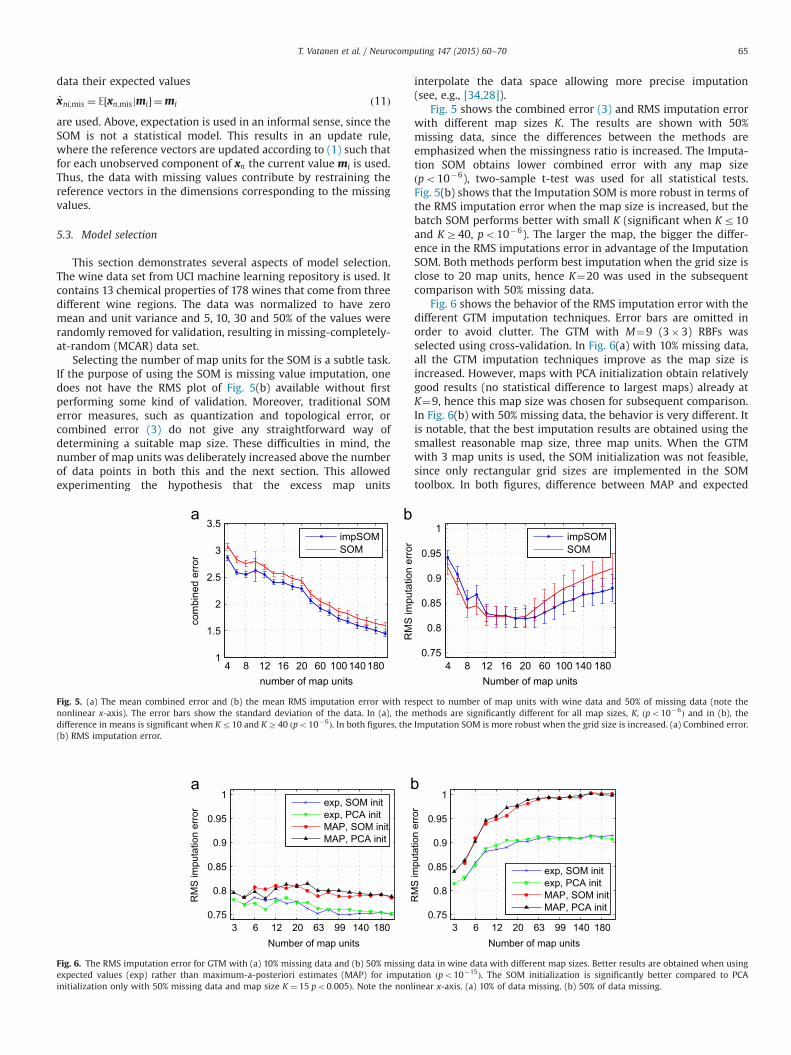
Fig. 5 shows the combined error (3) and RMS imputation errorwith different map sizes K. The results are shown with 50%missing data, since the differences between the methods areemphasized when the missingness ratio is increased. The Imputa-tion SOM obtains lower combined error with any map sizeðpo10�6), two-sample t-test was used for all statistical tests.Fig. 5(b) shows that the Imputation SOM is more robust in terms ofthe RMS imputation error when the map size is increased, but thebatch SOM performs better with small K (significant when Kr10and KZ40, po10�6). The larger the map, the bigger the differ-ence in the RMS imputations error in advantage of the ImputationSOM. Both methods perform best imputation when the grid size isclose to 20 map units, hence K¼20 was used in the subsequentcomparison with 50% missing data.

Fig. 6 shows the behavior of the RMS imputation error with thedifferent GTM imputation techniques. Error bars are omitted inorder to avoid clutter. The GTM with M¼9 (3�3) RBFs wasselected using cross-validation. In Fig. 6(a) with 10% missing data,all the GTM imputation techniques improve as the map size isincreased. However, maps with PCA initialization obtain relativelygood results (no statistical difference to largest maps) already atK¼9, hence this map size was chosen for subsequent comparison.In Fig. 6(b) with 50% missing data, the behavior is very different. Itis notable, that the best imputation results are obtained using thesmallest reasonable map size, three map units. When the GTMwith 3 map units is used, the SOM initialization was not feasible,since only rectangular grid sizes are implemented in the SOMtoolbox. In both figures, difference between MAP and expected

4 8 12 16 20 60 100 140 1801

1.5

2

2.5

3

3.5

number of map units

com

bine

d er

ror

impSOMSOM

4 8 12 16 20 60 100 140 1800.75

0.8

0.85

0.9

0.95

1

Number of map units

RM

S im

puta

tion

erro

r impSOMSOM

Fig. 5. (a) The mean combined error and (b) the mean RMS imputation error with respect to number of map units with wine data and 50% of missing data (note thenonlinear x-axis). The error bars show the standard deviation of the data. In (a), the methods are significantly different for all map sizes, K, ðpo10�6Þ and in (b), thedifference in means is significant when Kr10 and KZ40 ðpo10�6Þ. In both figures, the Imputation SOM is more robust when the grid size is increased. (a) Combined error.(b) RMS imputation error.

3 6 12 20 63 99 140 1800.75

0.8

0.85

0.9

0.95

1

Number of map units

RM

S im

puta

tion

erro

r exp, SOM initexp, PCA initMAP, SOM initMAP, PCA init

3 6 12 20 63 99 140 1800.75

0.8

0.85

0.9

0.95

1

Number of map units

RM

S im

puta

tion

erro

r

exp, SOM initexp, PCA initMAP, SOM initMAP, PCA init

Fig. 6. The RMS imputation error for GTM with (a) 10% missing data and (b) 50% missing data in wine data with different map sizes. Better results are obtained when usingexpected values (exp) rather than maximum-a-posteriori estimates (MAP) for imputation ðpo10�15Þ. The SOM initialization is significantly better compared to PCAinitialization only with 50% missing data and map size K ¼ 15 po0:005Þ. Note the nonlinear x-axis. (a) 10% of data missing. (b) 50% of data missing.

T. Vatanen et al. / Neurocomputing 147 (2015) 60–70 65

value imputation is significant for all K ðpo10�15Þ. In Fig. 6(b),there is still some evidence supporting the initialization with theSOM reference vector; when K¼15, the RMS imputation error isslightly better using the SOM initialization ðpo0:005Þ.

Table 1 summarizes the results of the experiments with thewine data set. One hundred randomly generated data sets witheach missingness ratio were imputed using all the methods.For each missingness ratio, the smallest map size whose result

was not statistically significantly worse than the best RMS impu-tation error, was chosen. The resulting map sizes were 63 (5%), 63(10%), 40 (20%), 40 (30%), 20 (50%) map units for the SOM and 99(5%), 99 (10%, SOM init), 9 (10%, PCA init), 4 (30%), 3 (50%, PCA init),4 (50%, SOM init) map units for the GTM. Topographic mappingsare compared with naive mean imputation and Variational Baye-sian PCA (VBPCA) [35], which can be used as a generic black boximputation even with extremely sparse data. Comparison with theVBPCA is used to evaluate the general usability of topographicmappings in missing value imputation tasks. VBPCA can performautomatic relevance detection (ARD), hence no model selection isneeded. We emphasize that more than two principal componentsare used in VBPCA. The mean result and its standard deviation inparentheses for each method and missingness ratio are listed. Thebest result(s) for each missingness ratio are in bold face.

The SOM methods and GTM with expectation imputationperform similarly except for 30% missingness ratio, when thedifference between the SOM methods and all GTM methods isstatistically significant ðpo0:01Þ. The GTM using the expectedvalues for imputation performs better compared to the MAPestimation of the missing values ðpo10�4Þ. The differencebetween VBPCA and the topographic methods is statisticallysignificant except for the 50% missingness ratio.

We also present the visualizations provided by these methodswhen operating with 50% missing data in the Figs. 7 and 8. Thegray-scale coloring behind the SOM Figs. 7(a) and (b) showU-Matrices of the maps. The three colors—blue, green and red—represent wines from three different wine regions, and the size ofthe colored markers in the SOMs is proportional to the number ofdata vectors mapped to the corresponding map unit.

For both SOMs in Fig. 7, the RMS imputation errors arerelatively close: 0.812 for the batch SOM and 0.803 for the

Table 1The means and the standard deviations (in parentheses) of the RMS imputationerrors for different imputation methods obtained by imputing a hundred data setswith randomly generated missing data and four missingness proportions using thewine data set. The best results for each missingness proportion is in bold face(including the results which do not differ from the best statistically significantly).SOM methods perform better compared to all GTM methods ðpo0:01Þ, whenmissingness proportion is 30%. (n) GTM expectation imputation performs bettercompared to MAP imputation for all missingness proportions (two last rows).

Method 5% 10% 30% 50%Missing Missing Missing Missing

Mean imputation 1.01 (0.06) 1.01 (0.05) 1.01 (0.03) 1.01 (0.02)

VBPCA 0.71 (0.06) 0.72 (0.04) 0.77 (0.03) 0.82 (0.02)

SOM 0.74 (0.07) 0.75 (0.05) 0.78n (0.03) 0.83 (0.02)ImpSOM 0.75 (0.07) 0.75 (0.05) 0.78n (0.03) 0.82 (0.02)

GTM exp, SOM init 0.75 (0.07) 0.75 (0.06) 0.79 (0.03) 0.82 (0.02)GTM exp, PCA init 0.75 (0.08) 0.76 (0.06) 0.79 (0.03) 0.82 (0.02)GTM MAP, SOM init 0.78 (0.07) 0.78 (0.06) 0.82 (0.03) 0.86 (0.03)GTM MAP, PCA init 0.79 (0.08) 0.80 (0.06) 0.82 (0.03) 0.84 (0.02)

Fig. 7. Clustering of the wine data set with 50% missing data using (a) the batch SOM and (b) the Imputation SOM. A SOM with 21(7�3) map was used. The size of thecolored markers is proportional to the number of data vectors mapped to the corresponding map unit. (a) SOM. (b) impSOM. (For interpretation of the references to color inthis figure caption, the reader is referred to the web version of this paper.)

T. Vatanen et al. / Neurocomputing 147 (2015) 60–7066

Imputation SOM. There are only minor differences between themaps produced by the batch SOM and the Imputation SOM.

According to the validation, an optimal number of map unitsfor the GTM with 50% missingness ratio equals 3, hence theresulting visualization, shown in Fig. 8(a), differs from the onesobtained using the SOM. Gaussian jitter is added to distinguishpoints in the figure. The latent points ui are assigned such thatthey form an equilateral triangle in the latent space; a configura-tion resembling the array of the hexagonal SOM. In the visualiza-tions, the distances between the units are proportional to theirdistances in the original data space, that is, dðui;ujÞpdðmi;mjÞ.The resulting RMS imputation error is 0.808. It is notable, that theGTM is able to provide results comparable with the SOM, withonly 3 map units. However, this is understandable since the dataactually consists of three different clusters, wines from threedistinct regions. Fig. 8(b) shows a GTM visualization using 20(5�4) map units. In this example, the RMS imputation errorequals 0.798, which is slightly lower compared to the GTM withthree map units. The same realization of missing values was used

in both figures. Furthermore, for this data the GTM with both PCAand the SOM initialization resulted in similar clustering. Onepossible explanation to this is, that the data lies close to the linearmanifold spanned by the two principal components which makeslearning the GTM model from the PCA initialization a feasible task.

To conclude this section, there seems to be small pieces ofevidence—more robust imputation with increased grid size andlower combined error—supporting the Imputation SOM over thebatch SOM. Regarding the GTM imputation, using the expectationof missing values proved to be the superior over the MAPestimates. This is natural, since using the MAP estimates discardinformation and is rarely a wise choice when dealing with multi-modal distributions.

5.4. ISOLET data

Finally, the methods are compared using the ISOLET dataintroduced in Section 4. Fig. 9 illustrates differences betweenthe Imputation SOM and the batch SOM. The values are based

Fig. 8. Clustering of the wine data set with 50% missing data using the GTMwith (a) 3, and (b) 20 (5�4) map units. Gaussian jitter is added in (a). (a) 3 map units. (b) 20 mapunits. (For interpretation of the references to color in this figure caption, the reader is referred to the web version of this paper.)

0 2000 4000 6000 800012

14

16

18

20

22

50 %

10 %

Number of map units

com

bine

d er

ror

impSOMSOM

0 2000 4000 6000 8000

0.65

0.7

0.75

0.8

50 %

10 %

Number of map units

RM

S im

puta

tion

erro

r impSOMSOM

Fig. 9. A comparison between the batch SOM and Imputation SOM algorithms with 10% (dashed line) and 50% (solid line) of MAR missing values in ISOLET data. Errors arecomputed using left-out validation data in 10-fold cross-validation and error bars show the standard deviation of results. (a) Combined error. (b) RMS imputation error.

T. Vatanen et al. / Neurocomputing 147 (2015) 60–70 67

on 10-fold cross-validation, where both error measures are eval-uated using left-out validation data, and the means and standarddeviations (error bars) over validation folds are shown. Differencesin combined error (3) increase when the map size is grown. Thehigher the proportion of missing data, the larger the difference interms of the combined error. Differences are highly significant(po10�5 for all K) when missingness proportion is 30% or 50% butis not significant ðp40:05Þ when 10% or 5% missing data is used.

There are significant differences error between the SOMmethods, with respect to RMS imputation error, only whenmissingness proportion is 50%. In that case, the batch SOMperforms significantly ðpo10�3Þ better imputation with smallmap sizes, when Kr1000, but the difference turns in favor of theImputation SOM when KZ7000.

Table 2 summarizes the results of the experiments with theISOLET data set. Ten randomly generated data sets with eachmissingness ratio were imputed using the SOM methods, VBPCAand mean imputation. For each missingness ratio, the smallestSOM map size, whose result was not statistically significantlyworse than the best RMS imputation error, was chosen. Theresulting map sizes were K¼8000 for all SOMs except the batchSOM with 50% missing data, in which case K¼4000. For all GTMs,the best map size was K¼3500. The results are reported on datanormalized to zero mean and unit variance.

The results with ISOLET data reveal more substantial differ-ences between the methods compared to the results in Table 1with the low-dimensional wine data. The GTM is excluded fromthe table, since we did not manage to thoroughly validate GTMparameters (K and M) for all missingness ratios, due to increasingcomputational burden when increasing the number of RBFs, M.However, the best results we obtained using the GTM withM¼400 (20�20) RBF centers were significantly worse than theSOM results in Table 2. For the GTM with SOM initialization thelowest obtained RMS imputation errors were greater than 0.7 andwith PCA initialization over 0.8. Differences between the SOMmethods are statistically significant with 30 and 50% missing data,but in practice the differences are negligible compared to thedifferences to VBPCA and the GTM. The best results were obtainedusing VBPCA, which determines the number of components byARD and more than two components (latent dimensions) wereused. This suggests that topographic mappings are not particularlysuitable for missing value imputation and it might be beneficial toimpute the data with any robust imputation method before theSOM or the GTM visualization.

6. Conclusions and discussion

In this paper, we have studied convergence properties of theSOM and the GTM and their behavior in the presence of missingdata. We also showed that initializing the GTM with the SOM maybe beneficial in some cases where the GTM with the conventional

PCA initialization fails to fit the data. This was demonstrated usingthe ISOLET, MNIST and ENCODE data sets. The initialization seemsto have very little effect with the wine data set, the data withlowest dimensionality used in our experiments.

We have also proposed a novel way of treating missingvalues in the SOM training called the Imputation SOM andshowed that this revision makes the SOM more robust in termsof the combined error (3) when missing values are present.The difference between the batch SOM and the Imputation SOMis emphasized when the map size is increased. However, when themain goal is to impute missing data, more well-founded ways,such as multiple imputation by chained equations (MICE) [36,37] orVBPCA, ought to be considered. In MICE, which is widely used inmissing value imputation tasks, each variable with missing data ischaracterized by a separate conditional linear model. In the case,where one aims at visualizing the data, one option (not investi-gated here) would be to first impute the data using anothermethod, and use the SOM or the GTM for the visualization taskafterwards. It was also shown that if the GTM is used for missingvalue imputation, expected values rather than MAP estimatesof missing values ought to be used. In the light of the imputationresults, it seems that the SOM initialization of the GTM improvesthe learning, but the GTM performs worse in terms of RMS impu-tation error compared to the SOM when using high-dimensionalISOLET data set.

Our experiments were not suitable for comparing the CPU timeconsumed by SOM and GTM since the GTM algorithm used in ourexperiments was not implemented having computational effi-ciency in mind. However, it is claimed in [3] that for bothalgorithms, the dominant computational cost arises from theevaluation of the Euclidean distances between data points andreference vectors. This was verified to be true for GTMs withrelative small number of RBFs ðMo100Þ using the Matlab Profiler,which measures where a program spends computational time.However, when the number of RBFs is increased, which was thecase in ISOLET imputation experiments in Section 5.4, the compu-tational cost becomes greater compared to the SOM.

In the future, it might be interesting to study whether the self-organization of the GTM benefits from sequential training. In ourinitial experiments, we have found that mini-batch training speedsup the convergence, as proposed by [21]. Additionally, theimprovements developed to enhance the self-organization of thebatch SOM may be applied for the GTM, as well. The number ofRBFs, M, roughly corresponds to the width of the neighborhoodfunction in the SOM. The smaller M, i.e. less RBFs, the more rigidthe mapping. Thus, the effect of annealed neighborhood may beachieved by increasing the number of RBFs during the learning. Itis also possible to use regularization, as was shown in [28], inorder to control the rigidness of the GTM.

References

[1] T. Kohonen, Self-organized formation of topologically correct feature maps,Biol. Cybern. 43 (1982) 59–69.

[2] T. Kohonen, Self-Organizing Maps, 3rd Edition, Springer-Verlag, Inc., New York,Secaucus, NJ, USA, 2001.

[3] C.M. Bishop, M. Svensén, C.K.I. Williams, GTM: the generative topographicmapping, Neural Comput. 10 (1) (1998) 215–234.

[4] J. Venna, S. Kaski, Local multidimensional scaling, Neural Netw. 19 (6–7)(2006) 889–899.

[5] S. Kaski, J. Kangas, T. Kohonen, Bibliography of self-organizing map (SOM)papers: 1981–1997, Neural Comput. Surv. 1 (3&4) (1998) 1–176.

[6] M. Oja, S. Kaski, T. Kohonen, Bibliography of self-organizing map (SOM)papers: 1998–2001 addendum, Neural Comput. Surv. 3 (1) (2003) 1–156.

[7] M. Pöllä, T. Honkela, T. Kohonen, Bibliography of Self-Organizing Map (SOM)Papers: 2002–2005 Addendum, Technical Report TKK-ICS-R23, Helsinki Uni-versity of Technology, 2009.

[8] An integrated encyclopedia of DNA elements in the human genome, Nature489 (7414) (2012) 57–74. URL http://dx.doi.org/10.1038/nature11247.

Table 2The means and the standard deviations (in parentheses) of the RMS imputationerrors for different imputation methods obtained by imputing 10 data sets withrandomly generated missing data and four missingness proportions using theISOLET data set. Differences between the SOM methods are significant with 30 and50% missing data (n). The VBPCA obtains the best result for each missingness ratio.

Method 5% 10% 30% 50%Missing Missing Missing Missing

Mean imputation 1.00 (0.03) 1.00 (0.02) 1.00 (0.01) 1.000 (0.01)VBPCA 0.42 (0.001) 0.42 (0.001) 0.44 (0.001) 0.47 (0.0003)SOM 0.64 (0.002) 0.64 (0.001) 0.652n (0.001) 0.669n (0.001)ImpSOM 0.64 (0.002) 0.64 (0.001) 0.654n (0.001) 0.665n (0.001)

T. Vatanen et al. / Neurocomputing 147 (2015) 60–7068

[9] A. Mortazavi, S. Pepke, C. Jansen, G.K. Marinov, J. Ernst, M. Kellis, R.C. Hardison,R.M. Myers, B.J. Wold, Integrating and mining the chromatin landscape of cell-type specificity using self-organizing maps, Genome Res. 23 (12) (2013)2136–2148, http://dx.doi.org/10.1101/gr.158261.113.

[10] T. Kohonen, P. Somervuo, How to make large self-organizing maps fornonvectorial data, Neural Netw. 15 (2002) 945–952.

[11] B. Hammer, A. Gisbrecht, A. Schulz, How to visualize large data sets?, in: P.A. Estévez, J.C. Príncipe, P. Zegers (Eds.), Advances in Self-Organizing Maps ofAdvances in Intelligent Systems and Computing, vol. 198, Springer, Berlin,Heidelberg, 2013, pp. 1–12.

[12] Y. Koren, The BellKor Solution to the Netflix Grand Prize, 2009.[13] J. Vesanto, J. Himberg, E. Alhoniemi, J. Parhankangas, Self-organizing map in

matlab: the SOM toolbox, in: The Matlab DSP Conference, 2000, pp. 35–40.[14] NETLAB: Algorithms for Pattern Recognition, Springer-Verlag New York, Inc.,

New York, NY, USA, 2002.[15] P. Koikkalainen, E. Oja, Self-organizing hierarchical feature maps, in: IJCNN,

vol. 2, 1990, pp. 279–285.[16] B. Fritzke, Growing cell structures—a self-organizing network for unsuper-

vised and supervised learning, Neural Netw. 7 (9) (1994) 1441–1460.[17] M. Dittenbach, D. Merkl, A. Rauber, The growing hierarchical self-organizing

map, in: IJCNN, 2000, pp. 15–19.[18] T. Villmann, R. Der, J.M. Herrmann, T. Martinetz, Topology preservation in self-

organizing feature maps: exact definition and measurement, IEEE Trans.Neural Netw. 8 (2) (1997) 256–266.

[19] L. Zhang, E. Merényi, Weighted differential topographic function: a refinementof topographic function, in: ESANN, 2006, pp. 13–18.

[20] S. Kaski, K. Lagus, Comparing self-organizing maps, in: Artificial Neural Networks(ICANN) 1996, vol. 1112, Springer, Berlin/Heidelberg, 1996, pp. 809–814.

[21] C.M. Bishop, C.K.I. Williams, Developments of the generative topographicmapping, Neurocomputing 21 (1998) 203–224.

[22] S. Haykin, Neural Networks and Learning Machines, 3rd Edition, Prentice Hall,Upper Saddle River, New Jersey, USA, 2008.

[23] K. Kiviluoto, E. Oja, S-Map: A network with a simple self-organization algo-rithm for generative topographic mappings, in: Advances in Neural Informa-tion Processing Systems, Morgan Kaufmann Publishers, San Francisco, CA,USA, 1998, pp. 549–555.

[24] J.-C. Fort, P. Letrémy, M. Cottrell, Advantages and drawbacks of the BatchKohonen algorithm, in: ESANN, 2002, pp. 223–230.

[25] A. Frank, A. Asuncion, UCI Machine Learning Repository, 2010. URL ⟨http://archive.ics.uci.edu/ml⟩.

[26] M.A. Fanty, R.A. Cole, Spoken letter recognition, in: NIPS, 1990, pp. 220–226.[27] T. Vatanen, I. Nieminen, T. Honkela, T. Raiko, K. Lagus, Controlling self-organization

and handling missing values in SOM and GTM, in: P.A. Estévez, J.C. Príncipe,P. Zegers (Eds.), Advances in Self-Organizing Maps of Advances in IntelligentSystems and Computing, vol. 198, Springer, Berlin, Heidelberg, 2013, pp. 55–64.

[28] T. Vatanen, Missing Value Imputation Using Subspace Methods with Applica-tions on Survey Data, Master's thesis, Aalto University, Espoo, Finland, 2012.URL ⟨http://users.ics.tkk.fi/tvatanen/online-papers/mthesis_vatanen.pdf⟩.

[29] F. Fessant, S. Midenet, Self-organising map for data imputation and correctionin surveys, Neural Comput. Appl. 10 (4) (2002) 300–310.

[30] S. Wang, Application of self-organising maps for data mining with incompletedata sets, Neural Comput. Appl. 12 (2003) 42–48.

[31] M. Cottrell, P. Letrémy, Missing values: processing with the Kohonen algo-rithm, in: Applied Stochastic Models and Data Analysis, 2005, pp. 489–496.

[32] R. Rustum, A.J. Adeloye, Replacing outliers and missing values from activatedsludge data using Kohonen self-organizing map, J. Environ. Eng. 133 (9) (2007)909–916.

[33] P. Merlin, A. Sorjamaa, B. Maillet, A. Lendasse, X-SOM and L-SOM: a doubleclassification approach for missing value imputation, Neurocomputing 73 (7–9)(2010) 1103–1108.

[34] A. Sorjamaa, Methodologies for Time Series Prediction and Missing Value Imputa-tion (Ph.D. thesis), Aalto University School of Science and Technology, Espoo,Finland, 2010.

[35] A. Ilin, T. Raiko, Practical approaches to principal component analysis in thepresence of missing values, J. Mach. Learn. Res. 99 (2010) 1957–2000.

[36] S. van Buuren, H.C. Boshuizen, D.L. Knook, Multiple imputation of missingblood pressure covariates in survival analysis, Stat. Med. 18 (1999) 681–694.

[37] S. van Buuren, K. Groothuis-Oudshoorn, MICE: multivariate imputation bychained equations in R, J. Stat. Softw. 45 (3) (2011) 1–67.

Tommi Vatanen is a Ph.D. student at Aalto University,Finland. He received his M.Sc. in bioinformation tech-nology in 2012 from Aalto University School of Elec-trical Engineering. He is also affiliated with BroadInstitute of MIT and Harvard in Cambridge, USA, wherehe is currently conducting research on human gutmicrobiome as a visiting graduate student.

Maria Osmala received the M.Sc. degree in bioinforma-tion technology from Aalto University School ofElectrical Engineering, Finland, in 2011. She is currentlya doctoral student in Department of Informationand Computer Science, Aalto University School ofScience, Espoo, Finland. Her research interests includeChIP-seq data analysis in epigenetics studies, regula-tory sequence prediction in human genome and datafusion in bioinformatics and computational systemsbiology.

Tapani Raiko received his D.Sc. degree in ComputerScience in 2006 from Helsinki University of Technology.He is an Assistant Professor (tenure track) and anAcademy Research Fellow at Aalto University Schoolof Science. His research focus is deep learning.

Krista lagus is a senior researcher, group leader, andPh.D. with experience in starting and leading researchand new innovation-oriented activities. She has writtenover 70 scientific publications. Developed jointly twosuccessful language technology methods and sofwareapplications, namely Websom and Morfessor. Started,planned and led EIT ICT Labs Wellbeing InnovationCamp 2010 and 2012.

Marko Sysi-Aho is a principal scientist and team leaderof the Biosystems modelling team at the Technicalresearch centre of Finland (VTT). He completed his Ph.D. in Computational Sciences at Aalto University in2005. His current research focus is on medical applica-tions of biosystems modelling, mainly related to devel-opment of methods for analysis and integration ofmetabolomics data with other data including environ-mental and life style factors.

Matej Orešič holds a PhD in biophysics from CornellUniversity. Since 2014 he is Principal Investigator atSteno Diabetes Center (Gentofte, Denmark), where heleads a Department of Systems Medicine. He is also anaffiliated group leader at the Turku Centre for Biotech-nology (Turku, Finland) and a principal investigator inthe Academy of Finland Centre of Excellence in Mole-cular Systems Immunology and Physiology Research.His main research areas are metabolomics applicationsin biomedical research and integrative bioinformatics.He is particularly interested in the identification ofdisease vulnerabilities associated with different meta-bolic phenotypes and the underlying mechanisms link-

ing these vulnerabilities with the development of specific disorders or theirco-morbidities, with specific focus on obesity and diabetes and their co-morbid-ities. He has also initiated the popular MZmine open source project, leading topopular software for metabolomics data processing. Prior to joining Steno DiabetesCenter, Dr. Orešič was research professor at VTT Technical Research Centre ofFinland (Espoo, Finland), head of computational biology and modeling at BeyondGenomics, Inc. (Waltham/MA) and bioinformatician at LION Bioscience Research inCambridge/MA.

T. Vatanen et al. / Neurocomputing 147 (2015) 60–70 69

Timo Honkela, Ph.D., is professor at the Department ofModern Languages at University of Helsinki. He hasconducted research on several areas related to knowl-edge engineering, cognitive modeling and natural lan-guage processing. This includes a central role in thedevelopment of the Websom method for visual infor-mation retrieval and text mining based on the Kohonenself-organizing map algorithm. Honkela is a formerlong-term chairman of the Finnish Artificial Intelli-gence Society.

Harri Lähdesmäki received the M.Sc. and D.Sc. degreesfrom Tampere University of Technology in 2001 and2005, respectively. Between 09/2002 and 03/2003, hewas a visiting researcher at the Cancer GenomicsLaboratory, The University of Texas M.D. AndersonCancer Center, and from 2005 to 2007 he worked as apostdoctoral fellow at the Institute for Systems Biology,Seattle, WA, USA. From 2007 to 2008, he worked as anAssistant Professor in the Department of Signal Proces-sing at Tampere University of Technology, Finland,followed by a pro term Professor position in HelsinkiUniversity of Technology until 2012. In autumn 2012 hewas appointed to Assistant Professor (tenure track) and

Academy Research Follow positions in the Department of Information andComputer Science at Aalto University School of Science (formerly known asHelsinki University of Technology). He is also an affiliated group leader at theTurku Center for Biotechnology, University of Turku. His research interests includecomputational and systems biology, regulatory genomics, statistical modeling andmachine learning, with applications to immunology, stem cell and T1D.

T. Vatanen et al. / Neurocomputing 147 (2015) 60–7070