SELLING ONLINE VERSUS LIVE - IDEI

SELLING ONLINE VERSUS LIVE

EIICHIRO KAZUMORI AND JOHN MCMILLAN

Abstract. Any seller choosing between auctioning online and livefaces a tradeoff: lower transaction costs online against more rentsleft with the bidders. We model this tradeoff, and apply the theoryto auctions of art. The crucial variable in determining whether theseller does better online is not the expected price but the extent ofvaluation uncertainty.

Online auction sales topped $50 billion in 2001. Cut flowers, seafood,classic cars, jewelry, coins, antiques, and art are now auctioned onlineas well as in traditional live sales. In what follows we model the seller’schoice of sale venue, online versus live, and apply the theory to auctionsof art, where prices and valuation uncertainties are the biggest of all.Are there limits to what can be sold online? Industry wisdom says

the internet is not suitable for selling highly valuable items, becausepotential buyers will resist bidding large sums for goods they havenot seen. Counterexamples exist, however. The town of Bridgeville,California was auctioned on eBay for $1.8 million. According to a newsreport, “Most of the 249 bidders made their offers based solely on digitalphotographs and descriptions of the town on a Web site.”1 A Ferrarisold on eBay Motors for $330,000; a 1909 baseball card sold on eBayfor $1.3 million; and an original of the Declaration of Independencesold on Sothebys.com for $8.1 million.There are two main differences between online and live auctions.

First, less information is available for bidders in online auctions. In alive auction, bidders inspect the item at the preview exhibition and (inthe case of art auctions) can ask questions of the auction-house expertspresent. In an online auction, bidders get only what information isposted on a web page. The fuzziness of pictures on a computer screenmeans an online bidder’s information is limited.

Date: January 11, 2003.Key words and phrases. auctions, electronic commerce.We acknowledge research support from the Center for Electronic Business and

Commerce at Stanford University Graduate School of Business and from a Stanforddissertation fellowship, and research assistance from Yee Man Chan, Brian Poi, andHa Quach.

1San Jose Mercury News, December 28 2002, p. 1A.1

2 EIICHIRO KAZUMORI AND JOHN MCMILLAN

Second, transaction costs are higher in live auctions. Online, theseller’s costs are those of running a web site. In live auctions, theauctioneer pays the costs of mounting the pre-sale exhibition and inrunning the theatrical performance that makes up a live auction. Theseller must wait until a suitable auction is scheduled, bringing costs ofdelay. Bidders have negligible transaction costs online, whereas to bidlive they incur travel and other participation costs.In the auctions of tuna at Tokyo’s Tsukiji market, where a single fish

goes for up to $15,000, buyers spend half an hour examining the tuna toassess their suitability for sashimi and sushi. This adds up to hundredsof person-hours of transaction costs in these live auctions. In onlineseafood auctions in Europe, by contrast, the auctioneer uses a letter-grade system to stipulate the freshness of the fish, economizing on thebidders’ time, possibly at the cost of inferior information. When Dutchflower auctions went online, prices fell–arguably because the internetbidders found it hard to assess the flowers’ quality.2

Any seller choosing between auctioning online and live, then, facesa tradeoff. On the one hand, the costs to the seller and the biddersof participating are lower online. On the other hand, online bidders,worrying more about the winner’s curse, bid lower. We will model thetradeoff of lower transaction costs online against more rents left withthe bidders.The internet has made markets more efficient by making it easier for

buyers to learn what is available where for how much. The loweringof these search frictions has made pricing more competitive, as vari-ous empirical studies have found (Baye, Morgan, and Scholten, 2001,Brown and Goolsbee, 2002, Brynjolfsson and Smith, 2000, Clay, Kr-ishnan, and Wolff, 2001, Ellison and Ellison, 2001). There is one set offrictions that the internet has not reduced, however: those of verifyingquality. Such frictions mean, we will argue, that online prices tend tobe less competitive.The winning bidder does better in an online auction than in a live

one, in our model, despite being more uncertain about the artwork’svalue (because competitors also bid lower). The gains can be mutual:in certain cases the seller, too, does better online.What are the limits of online auctions? The common belief among

online sellers seems to be that it is the item’s expected price that de-termines whether selling online works better for the seller; high-value

2On the Tsukiji fish auctions, see McMillan (2002, p. 65); on the online Euro-pean fish auctions, www.pefa.com/pefaportal/en/index.htm; on the Dutch flowerauctions, Koppius, Van Heck, and Wolters (2002).

ONLINE VERSUS LIVE 3

items should be sold live. Our theory suggests, to the contrary, thatthe crucial variable is not the expected price but the extent of valua-tion uncertainty. Valuable items can be successfully auctioned onlineif their variance of value is low.

1. Art Auctions

In 2000, Sotheby’s revamped its time-honored auction mechanism,when it started selling online via Sothebys.com. Any online seller ofheterogeneous goods faces questions of quality. The success of eBay, forexample, is in part due to its seller-reputation mechanism, reassuringbidders by tracking previous buyers’ experiences (Baron, 2001, Houserand Wooders, 2000, Lucking-Reiley, Bryan, Prasad, and Reeves, 2000,McDonald and Slawson, 2000, Resnick and Zeckhauser, 2001). Morethan anything else that is sold online, art is prone to vast uncertaintiesabout authenticity and merit. Art therefore tests the scope of onlinesales.Sotheby’s live auctions have four steps: consignment, cataloguing,

exhibition, and sale. After a prospective seller contacts Sotheby’s, itsexperts check the item’s authenticity and appraise its value. The ownerthen consigns the item to Sotheby’s, which puts it in an upcoming auc-tion. Sotheby’s auctions have a theme, such as “20th Century Worksof Art” or “Egyptian, Classical, and Western Asiatic Antiques,” sothe sale waits until there is an auction that it fits. The auction cat-alogue, available about one month ahead of the auction, contains adescription of the item, its history, reference notes, and an upper- andlower-bound estimated selling price. A few days before the auction,Sotheby’s mounts an exhibition of the items to be sold. The exhibi-tion is open the public and Sotheby’s specialists are on hand to answerquestions.3 Finally there is the auction itself, run with open ascendingbidding. Any major sale is a social event for the glitterati. Space in theauction room is scarce so it is rationed (Watson, 1992, p. 11), desirableseats being assigned to clients who have spent heavily in the past.Sotheby’s online auctions have a checkered history. Sothebys.com

began operations in January 2000 as a joint venture between Sotheby’s

3It is a case of buyer beware. A catalogue states, “Neither we nor the Con-signor make any warranties or representations of the correctness of the catalogue orother description of physical condition size, quantity, rarity, importance, medium,provenance, exhibitions, literature or historical relevance of the property and nostatement anywhere, whether oral or written, shall be deemed such a warranty orrepresentation. Prospective bidders should inspect the property before bidding todetermine its condition, size or whether or not it has been repaired or restored”(Sotheby’s, 1988).


and Amazon.com. This alliance was dissolved after nine months. (Theend came five days after Sotheby’s pleaded guilty to colluding withChristie’s to fix fees in their live auctions.) Sotheby’s operated theonline auctions its own from October 2000 to June 2002. During thistime it sold goods worth over $100 million in a period when the artmarket in general was depressed, but lost money because of the website’s high set-up costs.4 Then Sotheby’s formed a joint venture witheBay. The joint venture replaced eBay Premiere, eBay’s own site forhigh-end auctions, while Sotheby’s online business moved to eBay’sweb site, allowing Sotheby’s to cut staff and expenditures in its onlinedivision.The online auctions differ from the live auctions in several respects.

First, Sotheby’s is the consignor in only a fraction of Sothebys.comauctions. It has formed partnerships with about 5,000 “internet asso-ciates,” independent dealers who offer goods for sale at Sothebys.com.The associates authenticate their own goods and make their own ap-praisals. Second, rather than large auction events with specific themesat discrete times, miscellaneous items are continuously on offer via theweb site. (At any time the site lists around 13,000 items for sale.)Third, there is no printed catalogue and no exhibition; the descrip-tions are solely online. Fourth, the auction is run by eBay’s rules; inparticular, each auction has a fixed end-time (and so there is the possi-bility of last-second bidding, analyzed in eBay auctions by Bajari andHortacsu, 2002, and Ockenfels and Roth, 2002). Unlike eBay’s regu-lar auctions but like Sotheby’s live auctions, however, the online artauctions come with expert appraisals.Sotheby’s main cost of running online auctions is in producing the

web-site descriptions. This costs no more, presumably, than print-ing the catalogue for a live auction. The other live-auction costs areavoided. For bidders, participation is easier online. The live bidders’transaction costs go beyond travel and other pecuniary costs. Sotheby’sLondon and New York salerooms have an elitist ambiance, said to bedaunting to newcomers. “This world has been too intimidating and rar-ified,” said Sotheby’s president Diana D. Brooks when Sothebys.comwas starting up. “We want our site to be a friendly place to the po-tentially millions of people who’ve never bought art before.”5

An online bidder sees pictures of the item for sale, a paragraph ofbiography of the artist, a statement of the work’s condition, and a

4Sotheby’s incurred costs of $60 million in the first two years of its online oper-ation, mostly in set-up costs (Wall Street Journal, January 31, 2002, p. B4).

5Economist, January 27, 2000.


lower and upper estimate. Figures 1 and 2 exemplifiy how much–orhow little–information the bidders get. (To see more such examples,go to www.sothebys.com and click on a few of the items for sale.)The owner of a piece of art has a choice, then between selling it in a

live auction and online. Is the internet right for selling art? Sotheby’s

move to online auctions was greeted skeptically. Christie’s, Sotheby’srival in the global art-market duopoly, has deliberately stayed awayfrom online auctions. An unconvinced art dealer remarked, “What wesell is something that needs to be looked at and discussed.” The chiefexecutive of the US traditional art auctioneer Butterfields, Geoff Iddi-son, said, “Buyers expect to touch the works of art in person.”6 Nextwe develop a model that both sharpens and modifies the observationthat buyers prefer to see the art before bidding.

2. The Model and Equilibrium

The decision makers: The seller is defined by a unit endowment ofan asset with zero valuation and risk neutral preferences. A bidderi is defined by a scalar signal xi and risk-neutral preferences with anexpost payoff function s − p where s is the common value, and p isthe payment. (Risk aversion would reinforce the argument.) Definex = (x1, ..., xn). The seller and the bidders share a common prior on sand x.We model an online auction as a standard ascending auction—that is,

frictionless—and a live auction as having endogeneous entry of biddersand in which the seller and the buyers incur transaction costs.The decision process: First, nature decides a realization of s. Neither

the seller nor the bidders learns the realization of s. Second, the sellerdecides whether to sell the asset in online market or in offline market.Third, if the seller decides to sell the asset in online market. Then:

• The seller reveals information on the asset on the webpage. Theseller reveals information truthfully because of its guarantee7

and eBay’s feedback rating system.• Bidder i obtains the signal xoni from the distribution F on.• Bidders compete in an ascending auction. The seller put thereserve price ron ∈ R.

6The first quote is from a London oriental art dealer, Giuseppe Eskenazi: Econ-omist, January 27, 2000. Iddison quote: San Jose Mercury News, Aug. 2, 2002.7"Each seller guarantees that the authorship, period, culture or origin of the lot

is as set out in the Guaranteed sections of the View item page in the descriptionof the lot." and this guarantee is valid for three years for the bidder who purchasesthe asset. http://pages.sothebys.ebay.com/help/rulesandsafety/guarantee.html


Fourth, if the seller decides to sell the asset in a live auction:• The seller pays a cost cs ∈ (0, C) to hold a live auction.• The seller provides information on the asset in the auction cat-alogue. The information revelation is truthful8.

• Each potential bidder decides sequentially9 whether to enter theauction. At the time of the choice, each potential bidder readsthe catalogue. Each bidder learns the number of bidders whohave already entered the auction10

• If potential bidder i decides to enter, bidder i pays cost cb ∈(0, C) for some C ∈ R++. In an actual auction process, thebidders have to arrange the visit to the preview in New Yorkbefore inspecting the asset.

• Each bidder attends the preview and estimates the signal xoffi

from the distribution F off . Bidders learn the signal after theentry decision.

• Bidders compete in an ascending auction with a reserve priceroff .

The distributional assumptions: Each of Xoffi and Xon

i belongs to amean-dispersion family with a mean zero base random variable Z witha distribution function FZ and continuously differentiable density fZ

and with mean and dispersion parameters (µ, σoff ) and (µ, σon). (Forexample, if X is normal, the base random variable is N(0, 1).) Theassumption implies

F on(x) = FZ(x− µ

σon), F off(x) = FZ(

x− µ

σoff)

Intuitively, a member of mean—dispersion family is obtained by a shiftin mean µ and dispersion σ of the base distribution. Many distribu-tions, such as Gaussian, Poisson, uniform, lognormal, and extremumvalue distribution, satisfies this condition.

8An offline auction catalogue states, " We guarantee the authenticity of Author-ship of each lots contained in this catalogue... ’Authorship’, locations the identityof the creator, the period, culture, source of origin of property, as the case may be,as set forth in the Bold Type Heading of such catalogue entry."(Sotheby’s (1988))9Levin and Smith (1994) modelled simultaneous entry. There are no essential

differences between two formulations since both analysis are driven by bidder’s zeroprofit conditions. Other models include French and McCormick (1984), Hausch andLi (1993), McAfee, Quan, and Vincent (2002), and Ye (2001).10This information which might be available from the conversations with

Sotheby’s specialists when the potential bidders try to arrange a visit to the preview.


The signal (Xj1 , ...,X

jN ), j =on, off is independent. Further, we

assume the sensitivity of expected value to signal does not vary exces-sively with the level of the signal: that is, S and Xj, j =on, off aresuch that there exists m > 0,M <∞ such that for all x,

(2.1) m ≤ ∂

∂xiE[s|X = x] ≤M

(Recall affiliation already implies that E[s|X = x] is nondecreasingin each arguments.) For example, if m = M, a $1 increase in thesignal will increase the bidder’s expected value by the same amountregardless of the level of the signal. We assume both of Xoff

i , andXon

i satisfy increasing the hazard rate condition11.

Note that, if Yi,n is the ith highest realization out of n iid samples,then,

E(Y offi,n ) = µoff + σoffE(Y z

i,n), E(Yoni,n ) = µon + σonE(Y z

i,n).

For example, see David (1981, p. 129).The crucial parameter in our model, k, represents the extent to which

bidders are better informed about the asset’s value in a live auctionthan an online one. The live auction, we assume, provides a moreprecise signal: σoff = kσon for some 0 < k < 1. Here k measures thelower dispersion in live auctions compared with online; k = 0 impliescomplete elimination of dispersion and k = 1 implies zero reduction ofdispersion.The first result identifies the equilibrium of the model.Lemma 1: In online markets without reserve prices, each bidder’s

ex ante payoff is,

πonB =

ZHon(xi, N)(1− F on(xi))dxi

where

Hon(xi) ≡ZX−i

∂vi(x, x−i)∂x

|x=xif(x−i|xj ≤ xi, j 6= i)dx−i,

vi(x) = E[s|X = x].

The seller’s ex ante pected payoff is

πonS = Es−N

ZHon(xi, N)(1− F on(xi))dxi.

11The hazard rate of the random variable x is h(x) = f(x)/(1− F (x)).


In a live auction, the seller sets the reserve price equal to zero, andeach bidder’s ex ante payoff is zero. The seller’s expected payoff is

πoffS = Es− noffcb − cs

= Es− noffZ

Hoff (xi, noff)(1− F off (xi))dxi − cs.

where the number of bidders noff is determined endogenously byZHoff(xi, n

off )(1− F off(xi))dx = cb.

Recall the concept of marginal revenue introduced by Bulow andRoberts (1989) and Bulow and Klemperer (1996). In our setting, it is

MRi(xi) =−1f(xi)

d

dxi[vi(xi,x−i)(1− F (xi))].

We here suppress dependence on n unless needed. By our assump-tion, a bidder’s marginal revenue is monotone increasing in own signal.Thus the seller sells the asset to the bidder with the highest signal.Since we assume independent signals, the revenue equivalence theorem(Bulow and Klemperer (1996)) holds, so our results for online auctionsapply not only for ascending auctions, but also other standard auctionformats such as first price auctions and second price auctions.In a live auction, the number of bidders is determined so that the

ex ante profit is equal to zero. Otherwise, potential bidders will keepentering in the auction, and since bidder’s expected profit is strictly de-creasing in the number of bidders, the number of bidders is determined(ignoring integer constraints) by the zero profit condition.The tradeoff between online and live auctions is as follows. In a live

auction, the number of bidders, noff , can be less than the number ofbidders in an online auction, N . This will imply less competition. Onthe other hand, in the live auction, the information available to thebidders, Xoff , is more precise than in the online auction, Xon.Next, we provide three comparative-statics results on payoffs. These

results serve as a preliminary for the analysis in the next section andare of some theoretical interest by themselves. We first examine onlineauctions (i.e., standard auctions) in terms of dispersion parameters.Proposition 1: In an online auction, for any σ1 and σ2 such that

σ1 ≤ (m/M)σ2, the bidder’s expected profit is lower and the seller’sexpected profit is higher in an auction with σ1.An intuition is as follows: as σ falls, the bidders have a more precise

estimate of the asset, so they bid more aggressively. As a result, the


seller’s expected profit rises and the bidder’s expected profit decreases.A more quantitative intuition is that, the bidder’s expected profit iss function of the difference between the expected value of the highestsignal and the second highest signal. This difference is, by the formula(EY1,n − EY2,n) = σ(EZ1,n − EZ2,n), monotone decreasing in σ.This approach will provide a quantitative estimate of the change in

the expected profit as a function of dispersion. In contrast, previousresults such as Milgrom and Weber (1982b), Persico (1999), and Atheyand Levin (2001) are order-based.Next, we examine online auctions in terms of mean parameters.Proposition 2: In an online auction, the seller’s expected profit

and the bidder’s expected profit are independent of µ.An intuition is that bidder’s expected profit is determined by the

relative competition with other bidders. As a result, the mean shiftcommon to all bidders will not affect in the bidder’s payoff. Thus, theseller benefits totally from the increase in the mean parameter.Next, we examine live auctions (that is, auctions with endogenous

entry).Proposition 3: In a live auction, for any σ1 and σ2 such that

σ1 ≤ (m/M)σ2, the number of bidders will be monotone increasing andthe seller’s profit will be monotone decreasing in σ. The number ofbidders and the seller’s expected profit are independent of µ.The argument for the dispersion parameter is straightforward: when

the signal is less accurate, bidders bid more aggressively, so a bidder’s exante profit increases. Anticipating this, more bidders enter the auction.The added bidders do not, however, increase the seller’s revenue: thezero-profit condition means the seller’s payoff is equal to the value ofthe asset minus the bidder’s entry costs. The argument for the meanparameter is similar. Since the bidder’s ex ante expected payoff isindependent of the mean parameter, so is the number of bidders.

3. Live versus Online

Our main result shows that the choice between selling live and onlinemarkets depends upon three paramaters: µ, the item’s expected value,σ, the estimate variance, and k, the extent to which this variance islower live than online.Proposition 4: There exists k∗ < 1 such that for all k ≤ k∗, there

exist σ∗, µ∗ such that for all σ ≥ σ∗ and µ ≥ µ∗, the seller’s expectedprofit from selling live is higher than that from selling online.For an asset with a given mean and variance, therefore, an online

auction generates a higher return for the seller if k is close enough


to one, meaning the online bidders’ information is not too far inferiorto the live bidders’ information. The intuition is that, if the assethas high valuation risk, then the benefit from information revelationis higher in a live auction. Further, in this case, the difference in thenumber of bidders between the live and the online auction is smaller.Thus the seller prefers the live auction. Another way of saying thisis that the transaction cost is lower relative to the value of the asset.In a live auction, the seller has to pay not only her own transactioncosts but also, indirectly, the bidders’ participation costs (French andMcCormick, 1984; McAfee and McMillan, 1987). If the expected pricefrom a live auction does not cover these transaction costs, then theseller will not sell live.It is the nature of the item for sale that determines k : there is more

to be learned from seeing, say, an oil painting live rather than on acomputer screen reproduction than, say, a print. Thus the useful inter-pretation of Proposition 4 is that, for categories of assets with a given kparameter, online sales are justified for assets whose mean and varianceof value are not too high. High-value items can be sold online if k isclose enough to one.To see the role of the parameter k, consider how art differs from

financial assets. In the sale of a piece of art, the preview reduces thevaluation risk (k < 1). By contrast, staring at a 10,000 yen note willnot tell you anything about the risk of holding yen. As a result, thereis no merit in trading financial assets live, given the transaction costssaving from online trading.The force of the parameter k suggests that the limits of online auc-

tions differ for different categories of assets. The reproduction on acomputer screen of an oil painting, for example, loses much of thequality of the picture: the texture of the oil paint and the subtleties ofthe colors. For oil paintings therefore, k is likely to be close to zero,so online bidders would bid cautiously to avoid the winner’s curse, andlive auctions would tend to yield better returns for the seller. Withassets like coins and stamps, arguably, something closer to full infor-mation could be conveyed to online bidders, so k is close to one andthe limits of online auctions are reached later; an expensive asset witha small valuation risk can be successfully sold online if its k is not farbelow one. An example is the auction of an original of the Declarationof Independence for a record $8.14 million at Sothebys.com in 2000: aprinted document arguably has a k close to one.We now provide two simple numerical examples to explain our argu-

ment. Suppose the seller has an asset and wonders whether to sell it


online or liv. There are three bidders interested in the asset and eachbidder values the asset as an mean common value model

Pxi/3.

Example 1 : The seller estimates that the bidders will have signalsdistributed uniformly on [2,000, 18,000], based on the information theseller provides in the Internet. Alternatively, the seller could hold alive auction. In the live auction, the bidders need to pay $100 toattend the preview. The seller expects that information will be 75%more accurate in the sense that bidders will have signals distributeduniformly on [8,000, 12,000]. Should the seller hold a live auction ?Solution: First, we compute the seller and bidder profit from live

auctions. Consider a symmetric equilibrium where each bidder dropsout at the price equal to be value of the asset given the signal of thebidders who have already dropped out, and assuming all other remain-ing bidders having the same signal with that bidder. In expectation,bidder 1 has the signal $14,000, bidder 2 has $10,000, and bidder 3 has$6,000. Bidder 3 will drop out at $6000 (this simplification is not with-out loss of generality due to the linear structure of the model.) Bidder 3will drop out at $6,000. Bidder 2 will drop out at (6,000+10,000*2)/3= $8,667. The seller’s expected price is $8,666 and bidder’s ex anteexpected profit is (10,000-8,667)/3 = $433.Second, we compute the profits from a live auction. Suppose all

three bidders choose to enter the auction. In expectation, bidder1 has the signal of $11,000, bidder 2 $10,000, and bidder 3 $9,000.Bidder 3 should drop out at $9,000. Then bidder 2 drops out at(9,000+10,000*2)/3 = $9,666 dollars. The seller’s revenue is $9,666.The bidder’s ex ante expected payoff is 334/3 = $111. Given that,each of three bidders will enter the auction, since the ex ante expectedprofit of $111 is higher than the entry cost of $100.Third, we compute the seller’s decision. In an online auction, the

expected price is $8,667. In a live auction, the expected price is 9,667-100 = $9,556. Thus the seller will hold a live auction.Example 2 : The seller estimates that the bidder will have signals

distributed uniformly on [9,200, 10,800], based on the information onthe Internet. The seller can reduce the dispersion 75% to [9,800, 10,200]in a live auction. Should the seller hold a live auction?Solution: First, we compute the equilibrium payoffs. On average,

bidder 1 will have $10400, bidder 2 $10000 and bidder 3 $9600. Bidder 2will drop out at (9,600+20,000)/3 = $9,867. Thus the seller’s expectedprice is $9,867 and the bidder’s ex ante profit is 133/3 = $43.Second, we compute payoffs from a live auction [9,800, 10,200]. On

average, bidder 1 has $10,100, bidder 2 $10,000 and bidder 3 $9,900.Bidder 3 will drop out at (9,900+10,000*2)/3 = $9,966. The seller’s


expected price is $9,966 and the ex ante profit of the bidder is 34/3=$11. Given this profit, the third bidder will not enter. Then willtwo bidders enter? The price is $9,933, and the expected profit of eachbidder is 67/2 = $34. Thus the second bidder will not enter. Onlyone bidder will enter, and may bid a price of ε (depending on theformulation of bargaining between the seller and the bidder).Third, we derive the seller’s choice. The seller’s price from the online

auction is $9.867 and from the live auction. Thus the seller sellsonline.These examples show that dispersion of the estimates has a major

effect on the seller’s profit in common-value auctions. If the dispersionis large, the seller may hold a live auction, even given the participationcosts. If the dispersion is small, it may not pay to hold a live auction.Finally we look at differences in sale rates (that is, the percentage of

items that pass the reserve price and are sold):Proposition 5: The sale rate is higher in live auctions than in

online auctions.The intuition is that, in an online auction, since it is a standard

ascending auction, the seller sets nontrivial reserve price to increasethe sale price, thus creating a positive probability of no sale. In a liveauction, by contrast, since the seller’s profit is equal to social welfare netof transaction costs, the seller sets a zero reserve price and always sellsthe asset. (We could modify the model to generate the more realisticresult that the sale rate is less than 100 percent in live auctions bysupposing the seller has a positive value for the item unsold. The seller’svalue might, for example, be given as a draw from the distributionF offminus, perhaps, some constant to represent the seller’s need forliquidity. In such a model the sale rate would be less than 100 percentlive, but still lower online because of the reserve-price effect.)An alternative explanation is about the cost of resale. Holding an-

other auction is costly for offline auctions but costless for online mar-kets. As a result, the seller should be eager to trade the asset more ina live auction.Can a seller design an auction to combine the benefits of live and on-

line auctions? An alternative auction form, in between live and onlineauctions, is offered by both Sotheby’s and Christie’s: in live auctions,bidders may participate from a distance, by telephone, fax, or internet.The auction-house web sites offer the catalogues for live auctions andallow advance bids, which an auction-house employee will submit dur-ing the course of the live auction. There is even a provision in some liveauctions for real-time online bidding. Christie’s offers live streamingvideos, so that people can bid in live auctions from their computers.


From the seller’s point of view, however, this in-between alternativeoffers none of the saving in transaction costs of true online bidding.Even from a bidder’s point of view, our analysis implies, this is strictlyinferior. Bidders would do better participating either directly in alive auction or in a true online auction. Distant bidders, who havenot incurred the transaction costs entailed in seeing the piece of artfor themselves, are competing against the live bidders, who have seenit. Less-informed bidders, in common-value auctions in general, arehandicapped when competing against better-informed ones, and end upwith little or no net gain (Engelbrecht-Wiggans, Milgrom, and Weber,1983). When the artwork is of high value, they will be outbid by thebetter-informed live bidders; when it is of low value, they might win theauction but overpay. Online bidders in a live auction are in a no-winsituation. They can overcome this disadvantage by either inspectingthe item themselves at the presale exhibition or hiring an agent to dothe inspection; but this means incurring the same transaction costs asthe live bidders.

4. Art Auction Data

We now examine data from online and live art auctions in light of ourtheory. We collected data from the Sotheby’s and eBay websites usingPerl programs. The live-auction data are from Sotheby’s New Yorksales between June 1 and June 30, 2002 (representing 1,890 auctioneditems, with 1,213 successful sales and a total of $23,572,639 raised).The online auctions are transactions on the Sotheby’s site on eBaybetween June 26 and July 23, 2002 (representing 1,300 auctioned items,with 517 successful sales and a total of $68,2845 raised).Prices are much lower online than live. The mean selling price in

the live auctions is $18,801 and in the online auctions $1,483. Thehighest live-auction price in our sample is a George Graham timepiece,at $1,219,500; the highest online price is a Frank Lloyd Wright copperweed holder (that is, a vase) at $83,750. The lowest live-auction priceis a Cartier watch, at $358; the lowest online price is a drawing by aBritish artist, Nicole Hornby, at $11.50. Histograms of sales prices aregiven in Chart 1. Notice how skewed the distributions are: in bothonline and live auctions the vast majority of items sold are of relativelylow value.The types of items auctioned are compared in Table 1. For the live

auctions, this categorization is based on the auction titles. For theonline auctions, we use eBay’s categorization.


Live OnlineJewelry 635 73Paintings and sculpture 621 113Clocks and watches 562 41Antiques and furniture 286 233Books, prints 283 37Silver and ceramics 0 259Photos, stamps, coins 0 272Collectibles 0 356

Table1: Number of auctions by category

A higher percentage of successful sales in live auctions than on-line is predicted by our theory. The data are in accord with this. Over-all, the sale rate is 64.1% in live auctions and 39.7% in online markets.Table 2 shows the breakdown of sale rates by category. These salerates are roughly consistent with data from elsewhere. For example,eBay’s online art auctions in 2000 (in the Great Collections auctions,eBay’s predecessor to its Sotheby’s joint venture), the sale rate was 48%(Tully, 2000). At Christies London live auctions in 1995 and 1996, thesale rate was in the 70% to 80% range for paintings of various kinds,61% for photographs, 88% for clocks, and 86% for jewelry (Ashenfelterand Graddy, 2003).

Live OnlinePaintings & prints 83% 44%Watches & clocks 82% 63%

Jewelry 54% n.a.Furniture n.a. 66%Coins n.a. 80%Silver n.a. 80%Books 57% n.a.

Table2: Sale rates compared (n.a. means no dataavailable)

In auctions run under eBay’s rules, because of the fixed end-time, bidders usually submit bids very close to the closing time (Rothand Ockenfels, 2002). In our online-auction data, the mean timing ofa bid is made 78% through the period of auction; the median is atthe 96% point, and the 75th percentile is at the 99.7% point. In other


words, half of the bids, typically, are placed during the last 4% of thetime of the auction, and 25% in the last 0.3 percent of the auctionperiod. (See Chart 2.) Last-minute bidding, therefore, is prevalentnot only in lower-value eBay auctions but also in the art and antiquesauctions on Sothebys.com.Are the auctioneer’s presale estimates done honestly or strategically?

The existing evidence for live auctions is mixed. Ashenfelter (1989)found that auction houses are generally truthful, in that the meanof the high and low estimate is well correlated with the winning bid.Beggs and Graddy (1997) and Bauwens and Ginsburgh (2000), how-ever, found a tendency to systematically underestimate for some kindsof goods and overestimate for others. Mei and Moses (2002) offered evi-dence that estimates are strategically manipulated, expensive paintingsshowing an upward bias.The main result of our theory is that the decision to sell online rather

than live reflects the dispersion of bidder value estimates but not theirmean. It also reflects the extent to which the dispersion is reduced ifthe bidders can see the item live. We run a simple regression to testthis proposition. We use the auctioneer’s presale announcement of highand low price estimates to get a measure of the mean and dispersion.We take the mean of these two numbers to represent the mean of theestimate distribution, and the difference between them to represent thedispersion. Histograms of estimate means and dispersions, online andlive, are given in Charts 3 and 4.The highest mean estimate in our live auction data is a Pierre Fred-

erich Ingold timepiece, at $375,000 (it was sold); the highest in ouronline data is a Marilyn Monroe wedding gown, at $60,000 (unsold).The lowest mean estimate in our live auctions is a 1995 Cartier watch,at $600 (sold); the lowest in our online data is a Lee Tanner photographof John Coltrane, at $15 (unsold).The highest estimate dispersion in live auctions is the same Ingold

timepiece, at $250,000; the highest online also is the same item, theMarilyn Monroe wedding gown, at $20,000. The lowest estimate dis-persion in the live auctions is a Fouga wristwatch, at $100 (sold); online,the lowest is the same Tanner photograph, at $10.These cases suggest that the pre-auction estimate dispersion does

indeed reflect the degree of valuation uncertainty. A watch or photo isnot unique, so the history of prices of identical or similar items can beused to assess its value. Moreover, its value can be reasonably judgedfrom a written description plus a web-page reproduction. The value ofa deceased actress’s wedding dress, by contrast is harder to assess. It isunique, so its future resale value is highly uncertain. Moreover, it may


be hard to judge its quality from a web-page photograph: is it still ina good condition? Seeing it live may give a bidder significantly moreprecise information.These cases further suggest, as we would expect, that items with a

higher value show a higher dispersion of value estimates. This is thecase in our data. The correlation between the mean of the high and lowestimates and their difference is 0.9. The result of a probit regressionof the choice of online or live auction regressed on both mean anddispersion of estimates is given in Table 3. Despite the strong positivecorrelation between the two independent varioable, each is significantlydifferent from zero. Both the mean and the dispersion of estmatesmatter. Items with a high variance of value or a high mean value arelikely to be sold live rather than online.

Off Coefficient Standard Error z P>|z|EstAvg 0.0000686 0.0000135 5.09 0EstDiff 0.0000336 0.00000461 7.3 0Const -0.493068 0.0325403 -15.15 0

Obs 3180LR 1207.75

Prob>chi2 0PseudoR2 0.2801

Table3: Regression of online vs. liveauction

5. Simulation

In this section, we start the estimation of transaction costs and in-formation revelation by formulating qualitative response models.

5.1. A qualitative response model. We consider the decision of theseller regarding whether to sell the asset in online auctions or in liveauctions. We assume that the seller’s utility associated with the choiceof the auction is the expected profit πoffS and πonS plus an additive errorterm off and on. The data is the upper and the lower bound of theestimate x = [x, x]. The parameters we are interested in are transactioncosts cs and cb, and efficiency improvement k. Let θ = (c, k). Let Uoff

and Uon be the seller’s expected utility: Uoff = πoffS (x, θ) + off andUon = πonS (x) +

on.The basic assumption is that the seller sells the asset in a live auction

if Uoff ≥ Uon. Thus defining Off = 1 if the seller sells the asset in alive auction, we have


P (Off = 1) = P (Uoff ≥ Uon) = F (πoffS (x, x)− πonS (x, x, θ))

where F is the distribution function of off − on. The log likelihoodfunction is

logL =nXi=1

Offi logF (πonS (x)− πoffS (x, θ))

+nXi=1

(1−Offi) log(1− F (πonS (x)− πoffS (x, θ))).

The maximum likelihood estimatorˆ

θ is defined by ∂ logL∂θ|θ=

ˆθ= 0.

5.2. A simulation. The following simulation is based on very roughassumptions.First, in this draft, we use a very simple parametrization. Z=uniform

[−0.5, 0.5], X = µ+ σZ, ui(s, x) =P

xi/n where n is the number ofbidders.Second, compute the functional form of the discrete choice model

give above. In online auction12, since H(w,m) = F (w)n−1,

πB =1

n(EY1,n −EY2,n) =

σ

n(EY Z

1,n −EY Z2,n) =

σ

n(n+ 1)

πS = µ− nπB = µ− σ

(n+ 1).

Note the simple comparative statics result: the seller’s expected payoffis decreasing in the dispersion and increasing in the number of bidders.Given the smoothness, the consistency and asymptotic normality ofmaximum likelihood estimator is standard (Amemiya (1985), Section9.2.2.) The number of bidders is determined by kσ/n(n + 1) = cb.For simplicity, we approximate13 the solution of this equation by n =(kσ/cb)

0.5 to make a model linear in parameters. We set the number ofbidders in the online market be 2. Note 1860/1300=1.43 was an meannumber of bidders for online auctions. Thus we obtain

12We do not consider reserve prices in this estimation and simulation. It is easyto compute Bulow and Klemperer (1996) bounds.13The next version of the draft will give estimateion based on analytical solution

of this equation. Meanwhile, for reasonably large k, the differences between thesolution of x2 = k and x2 + x = k is small, for k = 10, the solution is 3.16228 and2.70156.


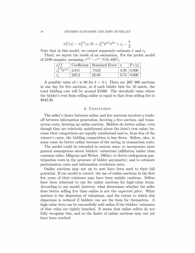
πonS (x)− πoffS (x, θ) = c0.5b k0.5σ0.5 + cs − σ

3.

Note that in this model, we cannot separately estimate k and cb.Third, we report the result of an estimation. For the probit model

of 3190 samples, assuming off − on˜N(0, 4002),off Coefficient Standard Error z P>|z|c1/2b k1/2 3.011 .7443 4.05 0.000cs 222.2 22.80 9.74 0.000

A possible value of c is 90 for k = 0.1. There are 200~300 auctionsin one day for live auctions, so if each bidder bids for 10 assets, thetotal bidding cost will be around $1000. The threshold value wherethe bidder’s rent from selling online is equal to that from selling live is$942.30.

6. Conclusion

The seller’s choice between online and live auctions involves a trade-off between information generation, favoring a live auction, and trans-action costs, favoring an online auction. Bidders do better online, eventhough they are relatively uninformed about the item’s true value, be-cause their competitors are equally uninformed and so, from fear of thewinner’s curse, the bidding competition is less fierce. Sellers, also, insome cases do better online because of the saving in transaction costs.The model could be extended in various ways: to incorporate more

general assumptions about bidders’ valuations (affiliation rather thancommon value: Milgrom and Weber, 1962a); to derive endogenous par-ticipation costs in the presence of bidder asymmetry; and to estimateparticipation costs and information revelation rates.Online auctions may not up to now have been used to their full

potential. If our model is correct, the use of online auctions in the firstfew years of their existence may have been unduly cautious. Sellershave been reluctant to opt for online auctions for high-value items.According to our model, however, what determines whether the sellerdoes better selling live than online is not the expected price. Whatmatters is the dispersion of valuations, and the extent to which thisdispersion is reduced if bidders can see the item for themselves. Ahigh-value item can be successfully sold online if the bidders’ estimatesof that value are tightly bunched. It seems that online sellers do notfully recognize this, and so the limits of online auctions may not yethave been reached.


References

[1] Ashenfelter, Orley (1989), How Auctions Work for Wine and Arts, Journal ofEconomic Perspectives 3(3).

[2] Athey, Susan (2000), Investment and Information Value for a Risk AverseFirm, preprint, Stanford.

[3] Athey, Susan and Philip A. Haile (2002), Identification of Standard AuctionModels, forthcoming, Econometrica.

[4] Athey, Susan and Jonathan Levin (2000), The Value of Information in Mono-tone Decision Problem, preprint, Stanford.

[5] Bajari, Patrick and Ali Hortacsu (2002), The Winner’s Curse, Reserve Pricesand Endogenous Entry: Empirical Insights from eBay Auctions, forthcoming,Rand Journal of Economics.

[6] Bajari, Patrick and Ali Hortacsu (2002), Cyberspace Auctions and PricingIssue: A Review of Empirical Findings, preprint, Chicago GSB.

[7] Barber, Brad M., and Terrance Odean (2000), Online Investors: Do the SlowDies First ?, forthcoming, Review of Financial Studies.

[8] Barber, Brad M., and Terrance Odean (2001), The Internet and the Investor,Journal of Economics Perspectives.

[9] Baron, David, Private Ordering on the Internet: The eBay Community ofTraders, preprint, Stanford GSB.

[10] Baye, Michael, John Morgan, and Patrick Scholten (2001), Price Dispersionin the Small and Large: Evidence from an Internet Price Comparison Site,preprint, UCB Haas.

[11] Beggs, A. and K. Graddy (1997): Declining Values and the Afternoon Effect:Evidence from Art Auctions. Rand Journal of Economics, 28, 544-65

[12] Brown, Jerry and Austan Goolsbee (2000), Does the Internet Makes MarketsMore Competitive ? Evidence from the Life Insurance Industry, Journal ofPolitical Economy 110 (3), 2002, 481-507

[13] Brynjolfsson, E., and Smith, M. (2000) Frictionless Commerce? A Comparisonof Internet and Conventional Retailers, Management Science, Vol. 46, No. 4

[14] Bulow, Jeremy and Paul Klemperer (1996), Auction versus Negotiations,American Economic Review 86(1), 180-93.

[15] Bulow, Jeremy and John Roberts (1988), The Simple Economics of OptimalAuctions, Journal of Political Economy.

[16] Carlton, Dennis and Judith A. Chevalier (2001), Free Riding and Sales Strate-gies for the Internet, Journal of Industrial Economics.

[17] Choi, James, David Laibson, and Andres Metrick, How Does the InternetAffect Trading, Evidence from Investor Behavior in 401(k) Plans, forthcoming,Journal of Financial Economics.

[18] David, Herbert (1981), Order Statistics, Wiley.[19] Ellison, Glenn, and Ellison, Sara F., Search, Obfuscation, and Price Elasticities

on the Internet, preprint, MIT, 2001.[20] Engelbrecht-Wiggans, Richard, Paul R. Milgrom, and Robert J. Weber, Com-

petitive Bidding and Proprietary Information, Journal of Mathematical Eco-nomics 11, 1983, 161-69.

[21] Forrester Research, eMarketplaces Will Lead US BusinesseCommerce to $2.7 Trillion in 2004, According to Forrester,http://www.forrester.com/ER/Press/Release/0,1769,243,FF.html


[22] French, Kenneth and Robert E. McCormick (1984), Sealed Bids, Sunk Costs,and the Process of Competition, Journal of Business 57(4), 417-441.

[23] Goolsbee, Austan (2000), Competition in the Computer Industry: Online ver-sus Retail, preprint, Chicago GSB.

[24] Goolsbee, Austan and Judith Chevalier (2002), Measuring Prices and PriceCompetition Online: Amazon and Barnes and Noble, preprint, Chicago GSB.

[25] Hallowell, Roger (2001), Sothebys.com, Harvard Business School 9-800-387.[26] Hasker Kevin, Raul Gonzalez and Robin Sickles (2001), An Analysis of Strate-

gic Behavior and Consumer Surplus in eBay Auctions, preprint, Rice.[27] Hausch, D.B., and L. Li (1993), A Common Value Auction Model with En-

dogenous Entry and Information Acquisition, Economic Theory 3(2), 315-334.[28] Herrmann, Frank (1980), Sotheby’s: Portrait of an Auction House, Chatto and

Windus.[29] Jackson, Matthew (2002), Efficiency and Information Aggregation in Auctions

with Costly Information, preprint, Caltech.[30] Koppius, Otto, Van Heck, Eric, and Wolters, Matthijs, “The Importance of

Product Representation Online: Empirical Results and Implications for Elec-tronic Markets,” unpublished, Erasmus University, Rotterdam, 2002

[31] Lacey, Robert (1998), Sotheby’s - Bidding for Class, Little, Brown and Com-pany.

[32] Levin, Dan and James Smith (1994), Equilibrium in Auctions with Entry,American Economic Review.

[33] McAfee, Preston and John McMillan (1987), Auctions with Entry, EconomicLetters 23, 343-47.

[34] McAfee, Preston, Daniel Quan, and Daniel Vincent (2001), How to Set Mini-mum Acceptable Bids, with An Application to Real Estate Auctions, preprint,Maryland.

[35] Milgrom, Paul (1981a), Good News and Bad News: Representation Theoremand Applications, Bell Journal of Economics.

[36] Milgrom, Paul (1981b), Rational Expectations, Information Acquisition, andCompetitive Bidding, Econometrica 49(4), 921-943.

[37] Milgrom. Paul (1991), Comparing Optima: Do Simplifying Assumptions AffectConclusions ?, Journal of Political Economy 102(2), 607-615.

[38] Milgrom, Paul and Ilya Segal (2002), Envelope Theorem for Arbitrary ChoiceSets, Econometrica.

[39] Milgrom, Paul and Robert J. Weber (1982a), A Theory of Auctions and Com-petitive Bidding, Econometrica 50(5), 1089-1122.

[40] Milgrom, Paul and Robert J. Weber (1982b), The Value of Information in aSealed-Bid Auction, Journal of Mathematical Economics 10, 105-114.

[41] Myerson, Roger (1982), Optimal Auction Design, Mathematics of OperationsResearch.

[42] Sandmo, Agnar (1971), On the Theory of the Competitive Firm under PriceUncertainty, American Economic Review, 61, 65-73.

[43] Shaked, Moshe and J. George Shanthikumar (1994), Stochastic Orders andTheir Applications, Academic Press.

[44] Sotheby’s (1988), Contemporary Prints: New York, Saturday, November 5,1988, Sotheby’s.


[45] Tully, Judd (2000), Upmarket eBay and Cyber Sotheby’s: Bidding on fine-art auction Web sites is taking an increasingly larger slice of the auction pie,http://www.cigaraficionado.com

[46] Watson, Peter, From Manet to Matisse: The Rise of the Modern Art Market,New York, Random House, 1992

[47] Wilson, Robert (1998), Sequential Equilibria of Asymmetric Ascending Auc-tions: the Case of Log-normal Distributions, Economic Theory.

[48] Ye, Lixin (2001), Optimal Auctions with Endogenous Entry, preprint, OhioState

7. Appendix: Proofs of the Propositions

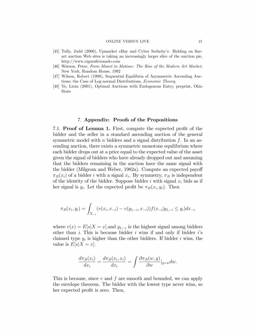
7.1. Proof of Lemma 1. First, compute the expected profit of thebidder and the seller in a standard ascending auction of the generalsymmetric model with n bidders and a signal distribution f . In an as-cending auction, there exists a symmetric monotone equilibrium whereeach bidder drops out at a price equal to the expected value of the assetgiven the signal of bidders who have already dropped out and assumingthat the bidders remaining in the auction have the same signal withthe bidder (Milgrom and Weber, 1982a). Compute an expected payoffπB(xi) of a bidder i with a signal xi. By symmetry, πB is independentof the identity of the bidder. Suppose bidder i with signal xi bids as ifher signal is yi. Let the expected profit be πB(xi, yi). Then

πB(xi, yi) =

ZX−i(v(xi, x−i)− v(y1,−i, x−i))f(x−i|y1,−i ≤ yi)dx−i

where v(x) = E[s|X = x].and y1,−i is the highest signal among biddersother than i. This is because bidder i wins if and only if bidder i’sclaimed type yi is higher than the other bidders. If bidder i wins, thevalue is E[s|X = x].

dπB(xi)

dxi=

dπB(xi, xi)

dxi=

Z∂πB(w, y)

∂w|y=wdw.

This is because, since v and f are smooth and bounded, we can applythe envelope theorem. The bidder with the lowest type never wins, soher expected profit is zero. Then,


πB(xi) =

Z xi

−∞

ZX−i

∂vi(w, x−i)∂w

f(x−i|y1,−i ≤ w)dx−idw

=

Z xi

−∞H(w, n)dw

(where H(w, n) ∼=ZX−i

∂vi(w, x−i)∂w

f(x−i|y1,−i ≤ w)dx−i.)

Then the bidder’s ex ante payoff is:

πB =

Z Z xi

−∞H(w, n)dwf(xi)dxi

= {Z xi

−∞H(w, n)dwF (xi) }+∞−∞ −

ZHi(xi, n)F (xi)dxi

=

ZH(w, n)dw −

ZHi(xi, n)F (xi)dxi

=

ZH(xi, n)dxi −

ZHi(xi, n)F (xi)dxi

=

ZH(xi, n)(1− F (xi))dxi.

The first line is by taking the expectation of πB(xi) and changing theorder of integration. The second line is by integration by parts. Thethird line is by integration by parts using the formula

Rab = [ab]−R a0b

with a =RH(w)dxi and b = F (x). The seller’s ex ante profit is the

difference between the item’s expected value and the bidders’ expectedprofits:

πS = Es− nπB

Second, we compute expected profits in an online auction without areserve price. From the previous formula, but with N bidders,

πonB =


πonS = Es−N


The number of bidders in the live auction is determined by the zero-profit condition (with bidders entering until profits are competed away,ignoring the integer constraint):


πoffB =

ZHoff (xi, n

off)(1− F off (xi))dxi = cb

The seller’s ex ante expected live-auction profit is

πoffS = Es− noffcb − cs

= Es− noffZ

Hoff (xi, noff)(1− F off (xi))dxi − cs.

7.2. Proof of Proposition 1. First, we claim that it is suffice to showthat bidder’s expected profit is lower in an auction with σ1 than onewith σ2. This is because the seller’s expected profit is the differencebetween the value of the asset and the bidders’ expected profit. (Bythe assumption of absolute common value, the value of the asset isindependent of σ.)Second, we compute the lower and upper bound of the bidder’s ex-

pected profit. Recall from Lemma 1, the bidder’s expected profit is

πB =

ZH(xi, n)(1− F on(xi))dxi.

Thus, from the definition of H and the assumption (*), πB is bounded:

m

ZF (xi)

n−1(1− F (xi))dxi ≤ πB ≤M

ZF (xi)

n−1(1− F on(xi))dxi.

The distributions and densities of the order statistics are (David, 1981):

F1,n(x) = F (x)n

F2,n(x) = F (x)n + nF (x)n−1(1− F (x))

f2,n(x) = n(n− 1)(1− F (x))F (x)n−1f(x)

and therefore a bidder’s expected profit can be written as:


ZF (xi)

n−1(1− F (xi))dxi = (1/n)

Zn(F (xi)

n−1 − F (xi)n)dxi

= (1/n)

Z(F2,n(xi)− F1,n(xi))dxi

= (1/n)

Zxi(f1,n(xi)− f(x2,n(xi))dxi

=1

n(EY1,n −EY2,n)

=σ

n(EZ1,n −EZ2,n).

where the third equality uses integration by parts, the fouth is bydefinition, and the last comes from the properties of mean-dispersionfamilies (where Z is the base random variable as defined above).Third, we show that the bidder’s profit is lower in auctions with

dispersion parameter σ1. The upper bound of the bidder’s profit froman auction with dispersion parameter σ1 is σ1M/n(EZ1,n−EZ2,n). Thelower bound is σ2m/n(EZ1,n − EZ2.n). Thus the bidder’s profit froman auction with σ1 is lower if

σ1M/n(EZ1,n −EZ2,n) ≤ σ2m/n(EZ1,n − EZ2.n)

which implies

(7.1) σ1 < (m/M)σ2.

7.3. Proof of Proposition 2. From Lemma 1, the bidder’s ex antepayoff is 1

n(EY1,n − EY2,n) =

σn(EZ1,n − EZ2,n), which is independent

of µ.

7.4. Proof of Proposition 3. First, we claim πB is monotone de-creasing in n. The seller’s profit is the highest marginal revenue amongbidders. Then the addition of one bidder weakly increases the seller’sprofit. This implies that the total surplus for the bidders decreases.Thus the bidder’s ex ante profit decreases.Second, we claim that n is monotone increasing in σ.The number

of bidders n is determined by the zero profit condition: πB(n, σ) = c.From the previous discussion, πB(n, σ) is monotone increasing in σ andmonotone decreasing in n. Thus n is monotone increasing in σ.Third, we claim that the seller’s expected profit is monotone de-

creasing in σ. From Lemma 1, the seller’s expected payoff is the valueof the asset minus the total payment of entry costs. By the absolute


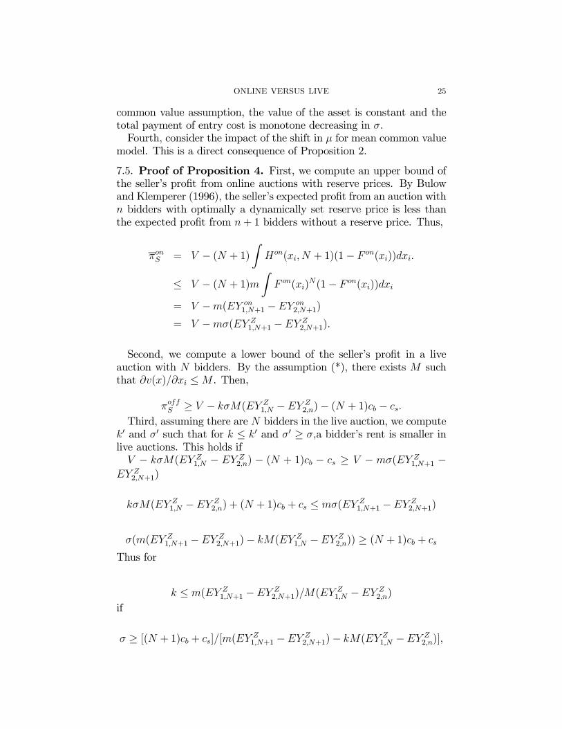
common value assumption, the value of the asset is constant and thetotal payment of entry cost is monotone decreasing in σ.Fourth, consider the impact of the shift in µ for mean common value

model. This is a direct consequence of Proposition 2.

7.5. Proof of Proposition 4. First, we compute an upper bound ofthe seller’s profit from online auctions with reserve prices. By Bulowand Klemperer (1996), the seller’s expected profit from an auction withn bidders with optimally a dynamically set reserve price is less thanthe expected profit from n+ 1 bidders without a reserve price. Thus,

πonS = V − (N + 1)

ZHon(xi, N + 1)(1− F on(xi))dxi.

≤ V − (N + 1)m

ZF on(xi)

N(1− F on(xi))dxi

= V −m(EY on1,N+1 −EY on

2,N+1)

= V −mσ(EY Z1,N+1 −EY Z

2,N+1).

Second, we compute a lower bound of the seller’s profit in a liveauction with N bidders. By the assumption (*), there exists M suchthat ∂v(x)/∂xi ≤M . Then,

πoffS ≥ V − kσM(EY Z1,N − EY Z

2,n)− (N + 1)cb − cs.

Third, assuming there are N bidders in the live auction, we computek0 and σ0 such that for k ≤ k0 and σ0 ≥ σ,a bidder’s rent is smaller inlive auctions. This holds ifV − kσM(EY Z

1,N − EY Z2,n) − (N + 1)cb − cs ≥ V − mσ(EY Z

1,N+1 −EY Z

2,N+1)

kσM(EY Z1,N −EY Z

2,n) + (N + 1)cb + cs ≤ mσ(EY Z1,N+1 −EY Z

2,N+1)

σ(m(EY Z1,N+1 −EY Z

2,N+1)− kM(EY Z1,N −EY Z

2,n)) ≥ (N + 1)cb + cs

Thus for

k ≤ m(EY Z1,N+1 −EY Z

2,N+1)/M(EYZ1,N −EY Z

2,n)

if

σ ≥ [(N + 1)cb + cs]/[m(EYZ1,N+1 −EY Z


2,n)],


the seller’s payoff is higher in live auctions.Fourth, we compute the conditions where there will be at least N

bidders in the live auction. This occurs if the bidder’s ex ante payoffwith N bidders is higher than the entry cost:πoffB ≥ m

RF on(xi)

N(1−F on(xi))dxi =mNkσ(EY Z

1,N+1−EY Z2,N+1) ≥

cb, That is,

σ ≥ Ncbmk(EY Z

1,N+1 −EY Z2,N+1)

Fifth, we compute the condition when both conditions are satisfied.For each k which satisfies k ≤ m(EY Z

1,N+1 − EY Z2,N+1)/M(EY

Z1,N −

EY Z2,n), there exists

σ ≥ max[ Ncbmk(EY Z

1,N+1 −EY Z2,N+1)

,(N + 1)cb + cs

m(EY Z1,N+1 −EY Z


2,n)]

where the seller’s profit is higher in a live auction. And if µ is highenough so that expected value of the allocation V (µ) is higher thancbN + cs,the seller will get a positive profit.

7.6. Proof of Proposition 5. First, compute the reserve price in anonline auction. In online auctions, by lemma 2 of Bulow and Klemperer(1996), the seller’s take-it-or-leave-it price is the price which makesmarginal revenue equal to zero. Thus, if the bidder with the highestmarginal revenue is less than zero, the seller does not trade.Second, compute the reserve price in a live auction. If the zero profit

condition is binding, the seller’s expected profit is equal to the expectedsocial surplus, thus the seller, who has the value zero for the asset, doesnot trade. If zero profit condition is not binding, then each bidder’smarginal revenue is strictly higher than that in an online auction, thusthe probability of exclusion is strictly lower.

California Institute of Technology and Stanford UniversityE-mail address: [email protected]

Current address: Stanford Graduate School of Business

Date post:	03-Feb-2022
Category:	Documents
Upload:	others
View:	1 times
Download:	0 times

SELLING ONLINE VERSUS LIVE - IDEI

Documents