Seminar Pavi

8/3/2019 Seminar Pavi

http://slidepdf.com/reader/full/seminar-pavi 1/30

MDPF For Search Applications In Mobile Adhoc Networks

Chapter 1

INTRODUCTION

In a Mobile Ad Hoc Network (MANET), mobile devices (nodes) may be spread over a large area

where access to external data is achieved through one or more access points(APs). However, not

all nodes have a direct link with these APs. Instead, they rely on other nodes that act as routers to

reach them. In certain situations, the APs may be located at the extremities of the MANET,

where reaching them could be costly in terms of delay, power consumption, and bandwidth

utilization. Additionally, the access point may connect to a costly resource (e.g., a satellite link),

or an external network that is susceptible to intrusion. For such reasons and others that concern

data availability and response time, MANET applications should check for the existence of the

desired data inside the network before attempting to connect to the external data source. An

example would be a node that is searching for data that have been requested before by other

nodes and are now cached and available to the rest of the nodes. Another example is where there

is a group of nodes that have data which may be of interest to other nodes and are willing to

share them. These scenarios and others suggest that efficient data search techniques be developed

for allowing mobile nodes to find the desired data if it exists in the MANET quickly and with

minimum power consumption. Given how ad hoc wireless networks work, searching

performance relies on the efficiency of employed routing strategies. Actually, one of the biggest

challenges in MANETS lies in the creation of efficient routing techniques [5].

Routing protocols are responsible for finding an efficient path between any two nodes in

the network that wish to communicate, and for routing data messages along this path. The path

must be chosen so that network throughput is maximized and message delay and other

undesirable events are minimized. Two main types of routing protocols exist: source routing and

destination routing. Destination routing itself is classified into two types: distance-vector routing,used in the RIP Internet protocol [11], and link-state routing, used in the OSPF Internet protocol

[12]. Relevant to our work are the Destination-Sequenced Distance Vector (DSDV) and the Ad

hoc On-demand Distance Vector (AODV) protocols, which are distance-vector routing protocols

designed for MANET environments. With such protocols, a node maintains a routing table and a

distance vector. The table contains the neighbor along the shortest path to each destination in the

Dept Of C.S.E, A.P.S.C.E 2010-11 Page 1




network, while the vector has the distance (number of hops) of this path. In high mobility

scenarios, the paths from sources to destinations will become nonoptimal (i.e., not the shortest

paths) until the routing tables are updated. With DSDV, each node periodically updates its

shortest paths by sending its distance vector to its neighbors to inform them about possible

distance changes to destinations in the network, while with AODV, a node computes/updates the

shortest path to a destination only when it needs to communicate with it (i.e., on demand).

Our proposed Minimum Distance Packet Forwarding (MDPF) algorithm is based on the

same basic concept employed by distance-vector routing protocols in that it forwards the search

message to the nearest node that potentially stores the desired data item. Actually, MDPF maybe

regarded as a high-level routing protocol operating on top of a distance-vector routing protocol,

and thus, together they form a two-layer protocol that works to minimize the response time of a

search application by following the consecutive shortest paths. The given analysis focuses on

providing confidence intervals for the mean distance to reach the node with the desired data and

the distance to traverse all the search nodes. Moreover, it will be demonstrated that MDPF

distributes the average load caused by search traffic among the visited nodes nearly uniformly in

spite of their possibly nonuniform caching capacities.

The rest of this paper is organized as follows: Section 2 describes the proposed approach

and illustrates it using an example application. Section 3 derives expressions for the system

parameters plus key performance measures and presents the analysis results. Section 4 presents

the simulations done using the ns2 software. Section 5 provides a short survey of related work,

while finally, Section 6 ends the paper with concluding remarks and ideas for future work.





Chapter 2

FRAMEWORK OVERVIEW

The idea behind MDPF is to use routing table information for visiting nodes in the order of

shortest distance (hop counts). As implied, this requires valid routing information, which could

be handled through a proactive routing protocol such as the DSDV protocol or an on-demand

reactive routing protocol, like AODV. We make the assumption that the set of nodes that hold

the search information is known to all nodes in the wireless network, and we refer to these nodes

as the search nodes, or SNs. We emphasize though that a requesting node which is interested in a

particular data item does not usually know which specific SN holds the location of the data item,

and therefore, it must search for it in the SNs.

2.1 Basic Operation

According to MDPF, the client uses the information in the routing tables to send its request

to the nearest SN. If an SN does not have the requested data, it also uses MDPF and forwards the

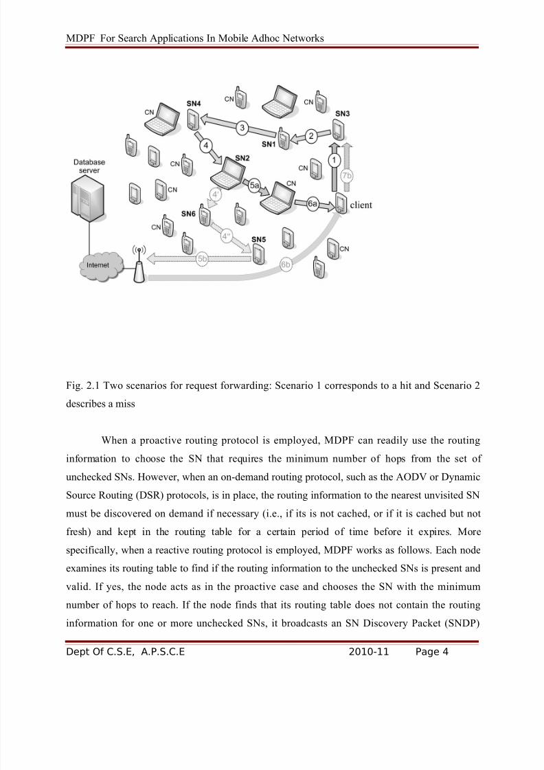
request to the nearest unvisited SN. Fig. 1 shows two example scenarios. Nodes request database

data, which may be cached in any of the caching nodes (CNs). The search nodes (SNs) cache

previously submitted requests (queries), and for each such query, an SN maintains a reference to

the result that resides on a CN. In the first scenario, the client submits its request to the nearest

SN (SN3), which does not have a matching query. The request is then forwarded in accordance

with MDPF through SN1 and SN4 before it arrives to SN2, where a match is found. Using the

reference that is stored along with the cached query, the request of the client is forwarded to the

CN that stores the result. This CN sends the result to the client whose address is found in the

forwarded packet. In the second scenario, no match is found in the SNs, and so, the last visited

SN (SN5) forwards the request to the data server via the access point. The server retrieves the

result and sends it directly to the client, which, in turn, asks SN3 (being its nearest SN) to cache

the query. It is noted that the node at which the client requested the data item that was retrieved

from the outside data server becomes a CN for this particular item.





Fig. 2.1 Two scenarios for request forwarding: Scenario 1 corresponds to a hit and Scenario 2

describes a miss

When a proactive routing protocol is employed, MDPF can readily use the routing

information to choose the SN that requires the minimum number of hops from the set of

unchecked SNs. However, when an on-demand routing protocol, such as the AODV or Dynamic

Source Routing (DSR) protocols, is in place, the routing information to the nearest unvisited SN

must be discovered on demand if necessary (i.e., if its is not cached, or if it is cached but not

fresh) and kept in the routing table for a certain period of time before it expires. More

specifically, when a reactive routing protocol is employed, MDPF works as follows. Each node

examines its routing table to find if the routing information to the unchecked SNs is present and

valid. If yes, the node acts as in the proactive case and chooses the SN with the minimum

number of hops to reach. If the node finds that its routing table does not contain the routing

information for one or more unchecked SNs, it broadcasts an SN Discovery Packet (SNDP)





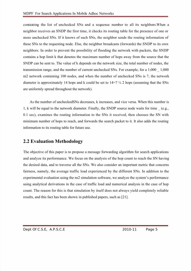
containing the list of unchecked SNs and a sequence number to all its neighbors.When a

neighbor receives an SNDP the first time, it checks its routing table for the presence of one or

more unchecked SNs. If it knows of such SNs, the neighbor sends the routing information of

these SNs to the requesting node. Else, the neighbor broadcasts (forwards) the SNDP to its own

neighbors. In order to prevent the possibility of flooding the network with packets, the SNDP

contains a hop limit k that denotes the maximum number of hops away from the source that the

SNDP can be sent to. The value of k depends on the network size, the total number of nodes, the

transmission range, and the number of current unchecked SNs. For example, for a 1;000 _ 1;000

m2 network containing 100 nodes, and when the number of unchecked SNs is 7, the network

diameter is approximately 14 hops and k could be set to 14=7 ¼ 2 hops (assuming that the SNs

are uniformly spread throughout the network).

As the number of uncheckedSNs decreases, k increases, and vice versa. When this number is

1, k will be equal to the network diameter. Finally, the SNDP source node waits for time _ (e.g.,

0.1 sec), examines the routing information to the SNs it received, then chooses the SN with

minimum number of hops to reach, and forwards the search packet to it. It also adds the routing

information to its routing table for future use.

2.2 Evaluation Methodology

The objective of this paper is to propose a message forwarding algorithm for search applications

and analyze its performance. We focus on the analysis of the hop count to reach the SN having

the desired data, and to traverse all the SNs. We also consider an important metric that concerns

fairness, namely, the average traffic load experienced by the different SNs. In addition to the

experimental evaluation using the ns2 simulation software, we analyze the system’s performance

using analytical derivations in the case of traffic load and numerical analysis in the case of hop

count. The reason for this is that simulation by itself does not always yield completely reliable

results, and this fact has been shown in published papers, such as [21].





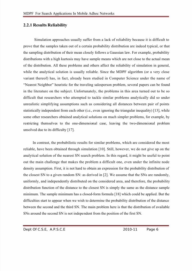
2.2.1 Results Reliability

Simulation approaches usually suffer from a lack of reliability because it is difficult to

prove that the samples taken out of a certain probability distribution are indeed typical, or thatthe sampling distribution of their mean closely follows a Gaussian law. For example, probability

distributions with a high kurtosis may have sample means which are not close to the actual mean

of the distribution. All these problems and others affect the reliability of simulation in general,

while the analytical solution is usually reliable. Since the MDPF algorithm (or a very close

variant thereof) has, in fact, already been studied in Computer Science under the name of

“Nearest Neighbor” heuristic for the traveling salesperson problem, several papers can be found

in the literature on the subject. Unfortunately, the problems in this area turned out to be so

difficult that researchers who attempted to tackle similar problems analytically did so under

unrealistic simplifying assumptions such as considering all distances between pair of points

statistically independent from each other (i.e., even ignoring the triangular inequality) [13], while

some other researchers obtained analytical solutions on much simpler problems, for example, by

restricting themselves to the one-dimensional case, leaving the two-dimensional problem

unsolved due to its difficulty [17].

In contrast, the probabilistic results for similar problems, which are considered the most

reliable, have been obtained through simulation [10]. Still, however, we do not give up on the

analytical solution of the nearest SN search problem. In this regard, it might be useful to point

out the main challenge that makes the problem a difficult one, even under the infinite node

density assumption. First, it is not hard to obtain an expression for the probability distribution of

the closest SN to a given random SN: as derived in [2]. We assume that the SNs are randomly,

uniformly, and independently distributed on the considered area, and therefore, the probability

distribution function of the distance to the closest SN is simply the same as the distance sample

minimum. The sample minimum has a closed-form formula [18] which could be applied. But the

difficulties start to appear when we wish to determine the probability distribution of the distance

between the second and the third SN. The main problem here is that the distribution of available

SNs around the second SN is not independent from the position of the first SN.





Indeed, since the second SN was the closest one to the first, it means that the second SN is on the

boundary of a disk centered at the first SN which is empty of any SN. As one reaches the third,

fourth, and nth SN, the empty area becomes an ever more complicated union of disks, making it

difficult to obtain a provably accurate analysis.

2.2.2 Implemented Methodology

To avoid the lack of reliability often associated with results obtained through simulations,

we will derive confidence intervals for the obtained results. For the numerical analysis, we will

be able to obtain results at the 0.0001 confidence level (meaning a probability inferior to

1/10,000 of being wrong), while maintaining an acceptable precision (between 10 and 30

percent). For the experimental evaluation, we will follow the lead of Andrel and Yasinsac [1]

and derive a sample size necessary to obtain a 90 percent confidence in the computed averages.

The next section describes two methods for implementing the numerical analysis for the hop

count measure, followed by a section that treats the analytical derivation of the average load

experienced by the SNs. Finally, a third section is dedicated to presenting the results of the

experimental evaluation.





Chapter 3

HOP COUNT ANALYSIS

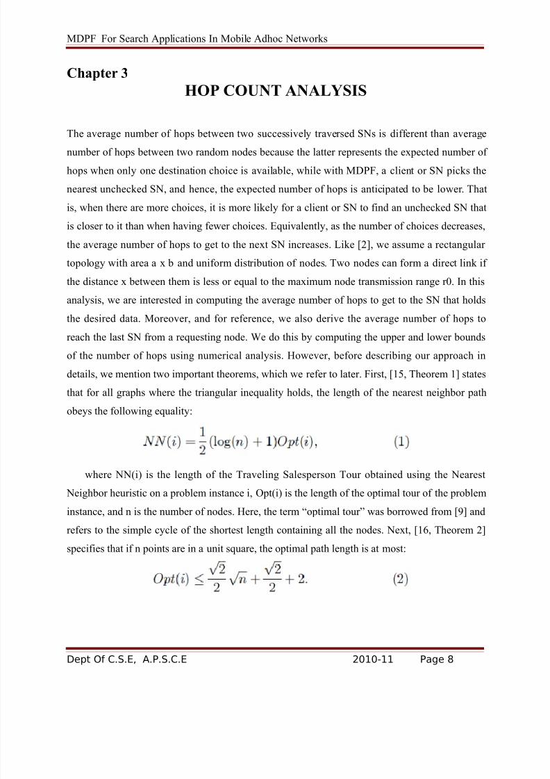
The average number of hops between two successively traversed SNs is different than averagenumber of hops between two random nodes because the latter represents the expected number of

hops when only one destination choice is available, while with MDPF, a client or SN picks the

nearest unchecked SN, and hence, the expected number of hops is anticipated to be lower. That

is, when there are more choices, it is more likely for a client or SN to find an unchecked SN that

is closer to it than when having fewer choices. Equivalently, as the number of choices decreases,

the average number of hops to get to the next SN increases. Like [2], we assume a rectangular

topology with area a x b and uniform distribution of nodes. Two nodes can form a direct link if

the distance x between them is less or equal to the maximum node transmission range r0. In this

analysis, we are interested in computing the average number of hops to get to the SN that holds

the desired data. Moreover, and for reference, we also derive the average number of hops to

reach the last SN from a requesting node. We do this by computing the upper and lower bounds

of the number of hops using numerical analysis. However, before describing our approach in

details, we mention two important theorems, which we refer to later. First, [15, Theorem 1] states

that for all graphs where the triangular inequality holds, the length of the nearest neighbor path

obeys the following equality:

where NN(i) is the length of the Traveling Salesperson Tour obtained using the Nearest

Neighbor heuristic on a problem instance i, Opt(i) is the length of the optimal tour of the problem

instance, and n is the number of nodes. Here, the term “optimal tour” was borrowed from [9] and

refers to the simple cycle of the shortest length containing all the nodes. Next, [16, Theorem 2]

specifies that if n points are in a unit square, the optimal path length is at most:





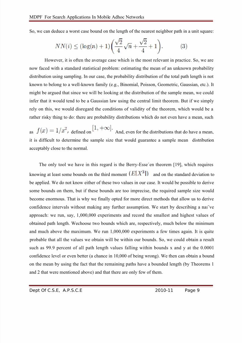
So, we can deduce a worst case bound on the length of the nearest neighbor path in a unit square:

However, it is often the average case which is the most relevant in practice. So, we are

now faced with a standard statistical problem: estimating the mean of an unknown probability

distribution using sampling. In our case, the probability distribution of the total path length is not

known to belong to a well-known family (e.g., Binomial, Poisson, Geometric, Gaussian, etc.). It

might be argued that since we will be looking at the distribution of the sample mean, we could

infer that it would tend to be a Gaussian law using the central limit theorem. But if we simply

rely on this, we would disregard the conditions of validity of the theorem, which would be a

rather risky thing to do: there are probability distributions which do not even have a mean, such

as defined on And, even for the distributions that do have a mean,

it is difficult to determine the sample size that would guarantee a sample mean distribution

acceptably close to the normal.

The only tool we have in this regard is the Berry-Esse´en theorem [19], which requires

knowing at least some bounds on the third moment and on the standard deviation to

be applied. We do not know either of these two values in our case. It would be possible to derive

some bounds on them, but if these bounds are too imprecise, the required sample size would

become enormous. That is why we finally opted for more direct methods that allow us to derive

confidence intervals without making any further assumption. We start by describing a naı¨ve

approach: we run, say, 1,000,000 experiments and record the smallest and highest values of

obtained path length. Wechoose two bounds which are, respectively, much below the minimum

and much above the maximum. We run 1,000,000 experiments a few times again. It is quite

probable that all the values we obtain will be within our bounds. So, we could obtain a result

such as 99.9 percent of all path length values falling within bounds x and y at the 0.0001

confidence level or even better (a chance in 10,000 of being wrong). We then can obtain a bound

on the mean by using the fact that the remaining paths have a bounded length (by Theorems 1

and 2 that were mentioned above) and that there are only few of them.





The main problem with this approach is that in spite of the very high confidence level it

guarantees, the bounds obtained are far too imprecise, since, in fact, all what we will have

established is a weaker form of the following statement: “We’re pretty sure that the mean must

be between the shortest path and the longest path we ever obtained.” This is why it was

necessary to come up with methods that trade off the confidence level for precision. In our work,

we obtained our confidence intervals using two methods, which can be combined or used

independently.

3.1 Method 1 for Computing the Confidence Intervals

If we call B the worst case path length, then to obtain a confidence interval for the mean, we

proceed as follows:1. Divide the interval [0, B] into n intervals b1; b2; . . . bn which need not all have the same size.

2. Run m experiments and record how often the path length falls within each interval.

3. Note that the function which maps the event that the path length falls within the ith interval is

a binomial random variable, since it has exactly two outcomes: either the path length falls within

the interval or it does not.

4. Estimate the parameter p, the proportion of the binomial distributions associated with each of

these n intervals, and obtain a confidence interval ci for each of these parameters using the

observed proportions during our experiments. We denote by li the lower extremity of the ith

confidence interval and ui its upper extremity. Clearly, our level of confidence, as guaranteed by

the Clopper Pearson method [6], that a given one of these intervals contains the actual value of

these parameters is not the same as our level of confidence that all these intervals contain their

corresponding parameters at the same time. The Clopper-Pearson method does not apply to the

latter situation, but we will see later how to deduce the level of confidence for the entire set of

intervals {b1; b2; . . . bn} from the level of confidence of the individual intervals. For the time

being we just assume that we are highly confident that all the parameters pi fall within their

computed confidence intervals. We let mi be the left extremity of bi and Mi its right extremity,

and let be the probability density function of the path length x.





We then have

Since we can make Mi × mi as small as we want, and since we can make li-ui arbitrarily

small provided that we can make the sample size arbitrarily large, we now have a method, which,

in principle, can yield results as precise as we want. But, in fact, the sample size would become

prohibitively large if the precision we require is too great.Aproblem remains: how are we going

to determine the confidence level of our estimation? We recall that a given procedure yields a

level of confidence α if the actual parameter falls within the confidence interval with a

probability of 1 -α.We now letA1 and A2 be two events with respective probabilities of 1 –α and

1 -β. We can write:

Therefore, the confidence level for the entire set ointervals is the sum of the confidence levels for

each interval. As expected, our confidence decreases as the number of interval decreases. Thus, it

appears that this is one possible method to trade confidence for precision.





3.2 Method 2 for Computing the Confidence Intervals

Our second method is based on the theorem that the sample mean is an unbiased estimator of

the mean, meaning that the probability distribution of the sample mean and the sampled

probability distribution have the same expectation. This theorem holds for all probability

distributions which have a finite mean. The motivation behind the use of the sample mean is that

as a consequence of the Central Limit Theorem, the sample means usually tend to be much more

tightly grouped than the sample values and this phenomenon increases with sample size.

While this is the reason why the confidence intervals we have obtained through this method

are relatively narrow, we do not rely on this fact to derive them. So, we proceed as follows:

1. First, decide the total number of experiments that we are going to perform, say N.2. Choose two numbers n1 and n2 such that n1× n2= N. The value of n1 will be the size of a

single sample and n2 will be the number of samples.

3. We run the N experiments, considering them to be n2 samples of n1 size each. We compute

the mean of each of the n2 samples. We get the smallest mean and the largest mean. We then

choose two bounds which are, respectively, say 5 percent smaller than the smallest mean and 5

percent larger than the largest mean.

4. We run the N experiments again. Hopefully, all the means will be within the bounds chosen in

step 3. If not, we keep widening the interval until all means are within it for several more runs of

the N experiments.

5. We are now able to obtain a good lower bound on the proportion of path lengths that lie within

the interval, with a high-level confidence, using the same basic principles as the Clopper Pearson

method.

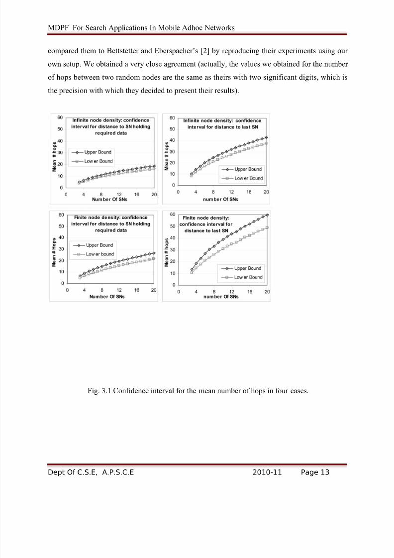
3.3 Confidence Intervals Computation Results

Using the two above methods, we obtained the confidence intervals for the path lengths, as

shown in Fig. 2. For each of these intervals, we are 99.9 percent sure that the mean falls within

them. In the infinite node density case, the sample size was 10,000, while for the finite density

case, the sample size was 3,000. All the corresponding bounds on the original distribution mean

are the 0.001 confidence level. To test the correctness and reproducibility of our results, we





compared them to Bettstetter and Eberspacher’s [2] by reproducing their experiments using our

own setup. We obtained a very close agreement (actually, the values we obtained for the number

of hops between two random nodes are the same as theirs with two significant digits, which is

the precision with which they decided to present their results).

Fig. 3.1 Confidence interval for the mean number of hops in four cases.





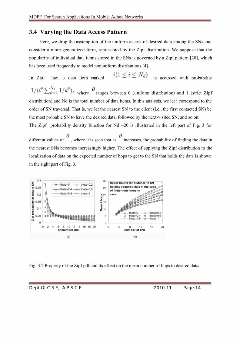
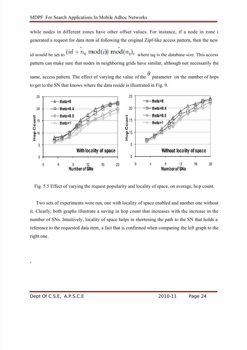
3.4 Varying the Data Access Pattern

Here, we drop the assumption of the uniform access of desired data among the SNs and

consider a more generalized form, represented by the Zipf distribution. We suppose that the

popularity of individual data items stored in the SNs is governed by a Zipf pattern [20], whichhas been used frequently to model nonuniform distributions [4].

In Zipf law, a data item ranked is accessed with probability

where ranges between 0 (uniform distribution) and 1 (strict Zipf

distribution) and Nd is the total number of data items. In this analysis, we let i correspond to the

order of SN traversal. That is, we let the nearest SN to the client (i.e., the first contacted SN) be

the most probable SN to have the desired data, followed by the next-visited SN, and so on.The Zipf probability density function for Nd =20 is illustrated in the left part of Fig. 3 for

different values of , where it is seen that as increases, the probability of finding the data in

the nearest SNs becomes increasingly higher. The effect of applying the Zipf distribution to the

localization of data on the expected number of hops to get to the SN that holds the data is shown

in the right part of Fig. 3.

Fig. 3.2 Property of the Zipf pdf and its effect on the mean number of hops to desired data.





Chapter 4

AVERAGE SEARCH NODE LOAD

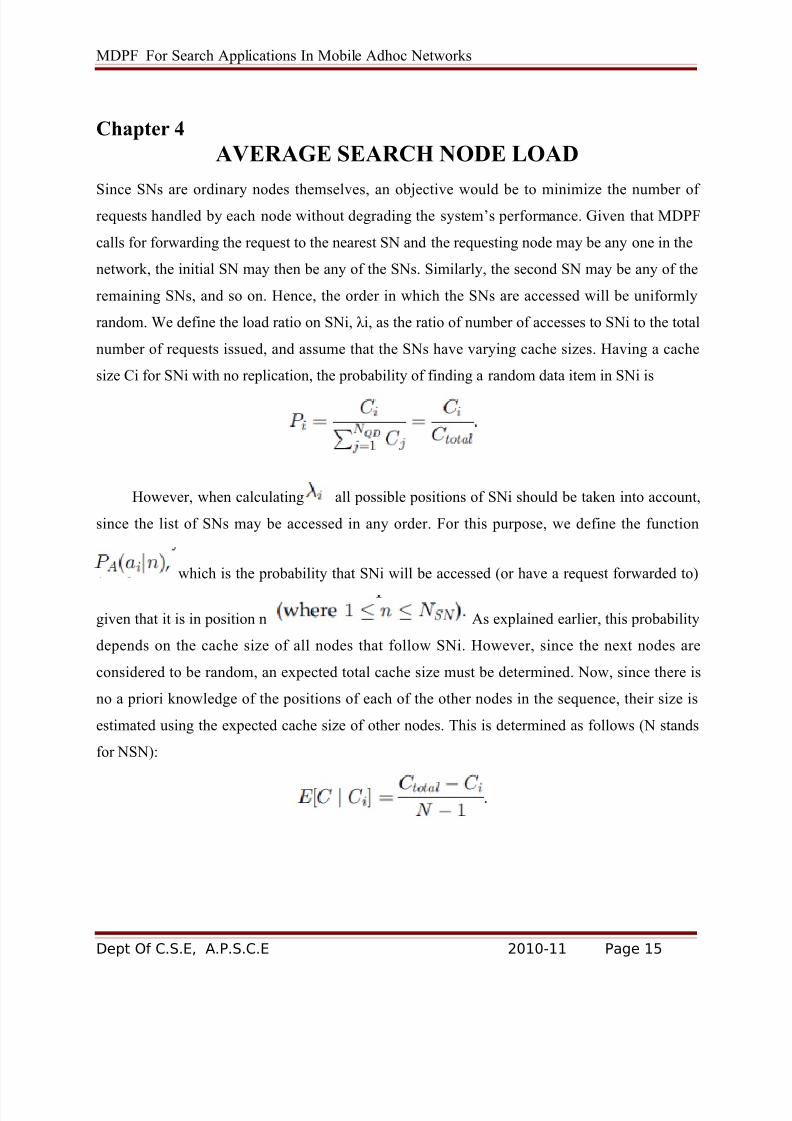
Since SNs are ordinary nodes themselves, an objective would be to minimize the number of requests handled by each node without degrading the system’s performance. Given that MDPF

calls for forwarding the request to the nearest SN and the requesting node may be any one in the

network, the initial SN may then be any of the SNs. Similarly, the second SN may be any of the

remaining SNs, and so on. Hence, the order in which the SNs are accessed will be uniformly

random. We define the load ratio on SNi, λi, as the ratio of number of accesses to SNi to the total

number of requests issued, and assume that the SNs have varying cache sizes. Having a cache

size Ci for SNi with no replication, the probability of finding a random data item in SNi is

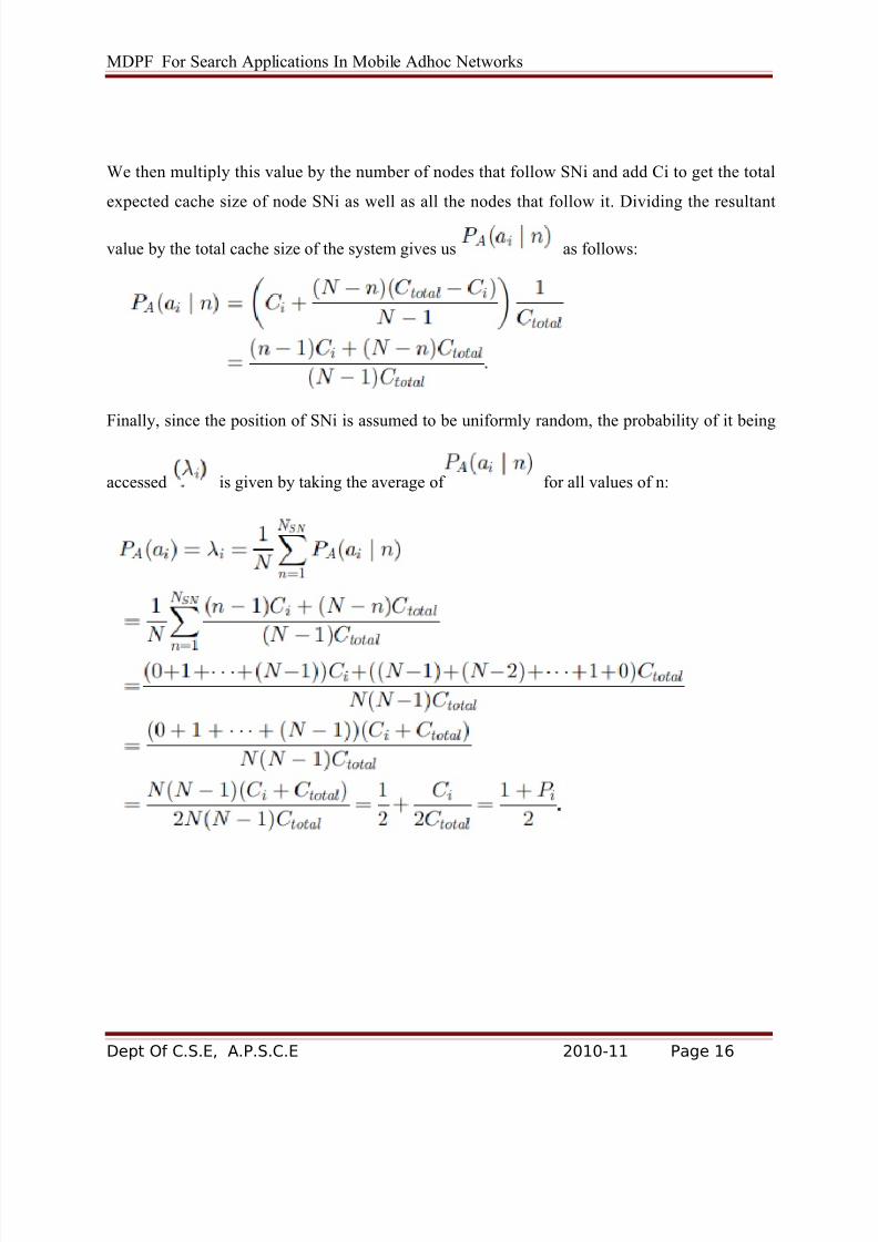
However, when calculating all possible positions of SNi should be taken into account,

since the list of SNs may be accessed in any order. For this purpose, we define the function

which is the probability that SNi will be accessed (or have a request forwarded to)

given that it is in position n As explained earlier, this probability

depends on the cache size of all nodes that follow SNi. However, since the next nodes are

considered to be random, an expected total cache size must be determined. Now, since there is

no a priori knowledge of the positions of each of the other nodes in the sequence, their size is

estimated using the expected cache size of other nodes. This is determined as follows (N stands

for NSN):





We then multiply this value by the number of nodes that follow SNi and add Ci to get the total

expected cache size of node SNi as well as all the nodes that follow it. Dividing the resultant

value by the total cache size of the system gives us as follows:

Finally, since the position of SNi is assumed to be uniformly random, the probability of it being

accessed is given by taking the average of for all values of n:





Fig. 4.1 Fraction of load per SN for two different storage capacity cases.

The expression in (11) is plotted in Fig. 4, where one SN has twice the cache size with

respect to the others, which, in turn, have the same size. The curves illustrate the load trends for

the SN with double the capacity and any of the other SNs, as the number of SNs increases. As

shown, the load starts high, especially for the double-capacity SN, and then, decreases toward a

lower bound. The curves illustrate that beyond a certain number of SNs, the benefit in terms of

lessening the load becomes insignificant, and also show that the lower limit of the load per SN is

0.5 when having a large number of SNs.





Chapter 5

EXPERIMENTAL EVALUATION

To experimentally evaluate MDPF, we implemented it and two other techniques to which we

compare it using the ns2 network simulation software. The other techniques are the Random

Packet Forwarding (RPF) and Minimal Spanning Tree Forwarding (MSTF) which we describe in

the section after next. This section presents the results and illustrates their significance.

5.1 NS2 Simulations Setup

We implemented MDPF, RPF, and MSTF on top of the proactive DSDV and the reactive

AODV routing protocols. In the simulated mobile ad hoc network, the wireless bandwidth and

the transmission range were set to 2 Mb/s and 100 m, respectively, while the topography size

was set to 750×750 m2. The network had 100 nodes randomly distributed in the topography and

their movement followed the Random Way Point movement model supported by ns2. The

default values of the minimum and maximum node velocity (Vmin and Vmax) were both set to 2

m/s and the node pause time to 100 seconds. Each node sends a request packet for a random data

item every 10 seconds. There are 10,000 data items that were disseminated uniformly across all

nodes at the beginning of the simulation.

For each data item, the nearest SN to the node holding the item is chosen to store the query

for that item along with the address of that node. To determine the hop count sample size that

would give a particular confidence level in the sample mean, we followed the procedure

described in [1]. Finding the sample size is not straightforward, especially in MANET

environments where there is considerable variation between “short” paths and “long” ones,

particularly in large to very large networks. Also, the number of short paths compared to that of

long ones depends on the distribution of nodes in the network and on the routing protocol used

and how it chooses the routing path between two nodes. Specifically, we used the procedure

explained in [1] to compute the number of simulation runs required for achieving at least a 90

percent confidence level in the presented results.





5.2 Description of Alternative Search Techniques

In RPF, the next SN to forward the search packet is chosen randomly from the list of

unchecked SNs, while in MSTF, the packet traverses the SN nodes which are connected via a

constructed minimal spanning tree (MST).The selected SN will then create an MST and send it to all SNs by unicast or multicast (the

simulations used multicast). Using this approach, a client can send its request to any of the SNs

(the nearest SN if the routing information is available). Then, the request is forwarded between

the SNs in accordance with the MST. Each SN that receives a request searches for its answer

(response) in its cache. If it finds the answer, it replies to the requester, else it sends the request

to the next unvisited SN along an MST edge (a list of visited SNs is included in the request

packet and updated at each visited SN). If an SN finds no SN along an MST edge to forward the

request to (for example, SN6 in Fig. 5), it sends the request to an unvisited SN along ordinary

routing paths.

Fig. 5.1 A sample MST connecting the SNs and a request traversing the SNs.

In the example of Fig. 5, a request is sent to SN1, then to SN2, SN4, SN5, and SN6 along the

edges of the MST. At SN6, the request needs to be forwarded to a next unvisited SN along the

MST. However, such SN doesn’t exist. Hence, SN6 will forward the request to one of the

remaining unvisited SNs (SN3 and SN7) along routing paths available from the routing protocol.

If such paths don’t exist, SN6 will send the request along the reverse path it came from (i.e, to





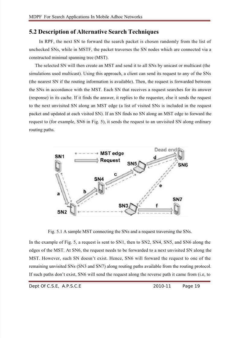
SN5, SN4, then SN2) until the request reaches an SN that has a path to one of the remaining

unvisited SNs. Note that the reverse path can be determined by the order of visited SNs in the

request packet. In MSTF, even though an MST builds a tree that links all its nodes with the least

number of total hops hMST , the total number of hops traversed by the packet, however, could be

greater than hMST due to the aforementioned condition, and as illustrated in the example of Fig.

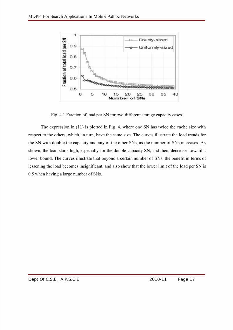
5. However, we will illustrate later in this section that MSTF might produce better average

search times when the time to search for the data item at an SN is significantly high.

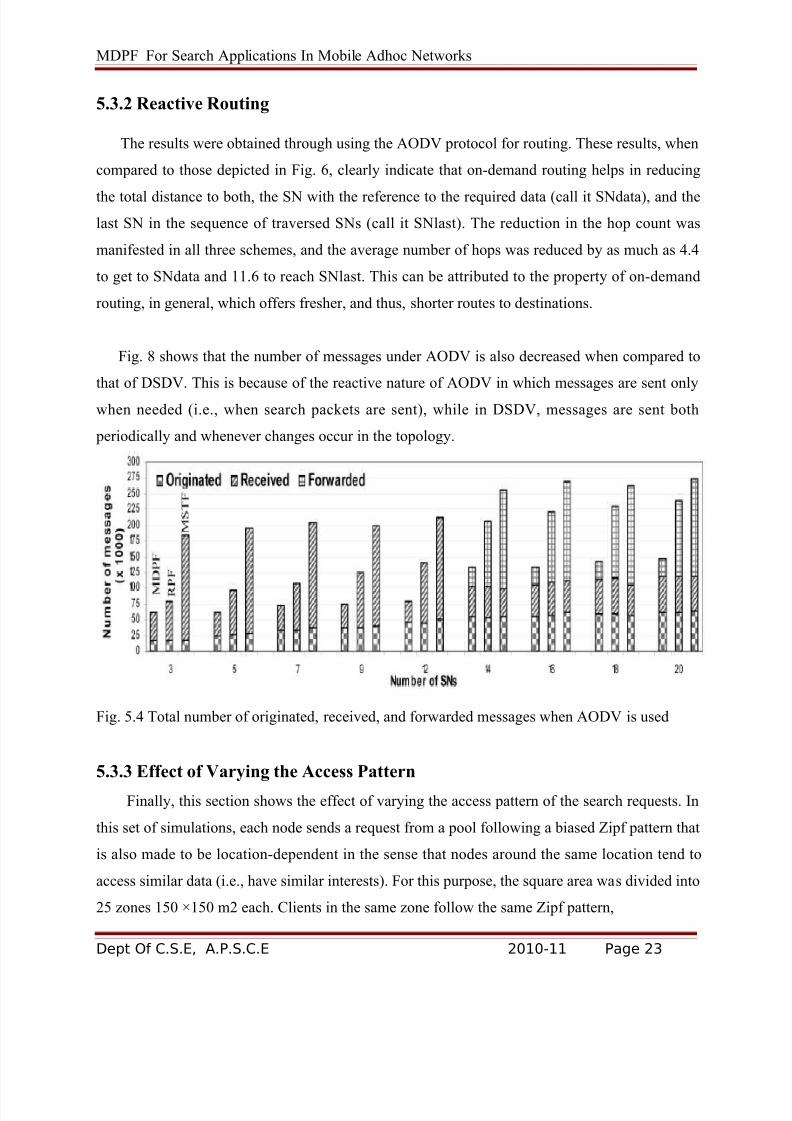
5.3 Results

To be consistent with the results presented in Section 3.5, we computed the lower and upper

bounds of the mean hop count for each scenario, in addition to the average taken over all sample

values. As was described above, each experiment comprised at least 27,000 points. To compute

the bounds, we used a procedure that is similar in principle to Method 2 (see Section 3.1.2) by

dividing the sample space into 54 groups, each consisting of about 500 samples. For each group,

the average value was computed, and then, the lower and upper bounds were taken as the lowest

and highest means, respectively, across all groups. In addition to the bounds, the overall average

was taken over all 27,000 points.

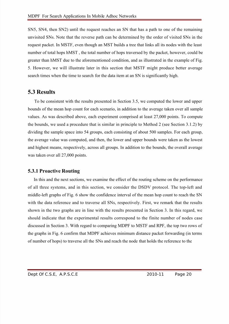
5.3.1 Proactive Routing

In this and the next sections, we examine the effect of the routing scheme on the performance

of all three systems, and in this section, we consider the DSDV protocol. The top-left and

middle-left graphs of Fig. 6 show the confidence interval of the mean hop count to reach the SN

with the data reference and to traverse all SNs, respectively. First, we remark that the results

shown in the two graphs are in line with the results presented in Section 3. In this regard, we

should indicate that the experimental results correspond to the finite number of nodes case

discussed in Section 3. With regard to comparing MDPF to MSTF and RPF, the top two rows of the graphs in Fig. 6 confirm that MDPF achieves minimum distance packet forwarding (in terms

of number of hops) to traverse all the SNs and reach the node that holds the reference to the





Fig. 5.2 Mean number of hops and total search times when DSDV routing is used.





requested data item. On the other hand, when considering the local search time (Tls) at each SN,

MSTF will take less total time when Tls is greater than 10 milliseconds, as illustrated in the

bottom graph of Fig. 6. This is because the savings in the cumulative forwarding time become

outweighed by the much larger total search time. Note that the forwarding time in the three

systems was set to 5 milliseconds, which is the average communication time between two nodes.

Finally, Fig. 7 shows the total number of messages generated during the simulation time by

the three systems for different numbers of SNs. It is noticed that MDPF generates the least

number of messages (requests, replies, and control packets), because the nearest SN is always

chosen. Furthermore, the number of messages successfully reaching their destinations is higher

in MDPF than that in RPF, which is why the number of received messages for MDPF is higher

than that of RPF. Finally, MSTF generates a large number of control messages (MST and routing

table messages) that are sent periodically, which is why the number of originated, received, and

forwarded messages is much greater in MSTF.

Fig. 5.3 Total number of originated, received, and forwarded messages when DSDV is used.





5.3.2 Reactive Routing

The results were obtained through using the AODV protocol for routing. These results, when

compared to those depicted in Fig. 6, clearly indicate that on-demand routing helps in reducing

the total distance to both, the SN with the reference to the required data (call it SNdata), and the

last SN in the sequence of traversed SNs (call it SNlast). The reduction in the hop count was

manifested in all three schemes, and the average number of hops was reduced by as much as 4.4

to get to SNdata and 11.6 to reach SNlast. This can be attributed to the property of on-demand

routing, in general, which offers fresher, and thus, shorter routes to destinations.

Fig. 8 shows that the number of messages under AODV is also decreased when compared to

that of DSDV. This is because of the reactive nature of AODV in which messages are sent only

when needed (i.e., when search packets are sent), while in DSDV, messages are sent both

periodically and whenever changes occur in the topology.

Fig. 5.4 Total number of originated, received, and forwarded messages when AODV is used

5.3.3 Effect of Varying the Access Pattern

Finally, this section shows the effect of varying the access pattern of the search requests. In

this set of simulations, each node sends a request from a pool following a biased Zipf pattern that

is also made to be location-dependent in the sense that nodes around the same location tend to

access similar data (i.e., have similar interests). For this purpose, the square area was divided into

25 zones 150 ×150 m2 each. Clients in the same zone follow the same Zipf pattern,





while nodes in different zones have other offset values. For instance, if a node in zone i

generated a request for data item id following the original Zipf-like access pattern, then the new

id would be set to where nq is the database size. This access

pattern can make sure that nodes in neighboring grids have similar, although not necessarily the

same, access pattern. The effect of varying the value of the parameter on the number of hops

to get to the SN that knows where the data reside is illustrated in Fig. 9.

Fig. 5.5 Effect of varying the request popularity and locality of space, on average, hop count.

Two sets of experiments were run, one with locality of space enabled and another one without

it. Clearly, both graphs illustrate a saving in hop count that increases with the increase in the

number of SNs. Intuitively, locality of space helps in shortening the path to the SN that holds a

reference to the requested data item, a fact that is confirmed when comparing the left graph to the

right one.

.





Chapter 6

RELATED WORK

Several works have tackled the problem of traversing a certain set of nodes in a network

according to some given criteria. We begin with Espes and Mammeri who propose in [7] an

adaptive expansion search method, in which nodes in the network determine their locations using

a Global Positioning System (GPS). The route request packet is sent only to nodes within a

certain triangle whose vertex is S (source node), height SD+ and angle (where SD is the

distance between source and destination nodes, while and are the dynamically changing

parameters).

Each source node sends a route request with starting values of and to nodes lying within

the search triangle, and then, sends another route request with new (greater) values after a certain

timeout (hence expanding the search triangle), and so on. The reported results show that the

proposed system always returns a valid route after a given number of attempts. An approach to

using Dynamic Hash Tables (DHTs) in distributed applications within MANETs was proposed

in [14].

The approach includes two methods: The first usesDHTs on top of an MANET routing

protocol, and hence, it requires provisions for communication and control messages exchange

between the DHT algorithm and the routing protocol. The second method integrates the DHT

into the routing protocol itself such that the next destination for each message is obtained from

the DHT (for maximum efficiency), while the routing path of the message is obtained from the

routing protocol. The authors do not describe in details how a DHT can generally be integrated

into a particular routing protocol (for example, how different DHTs can be incorporated into

different types of routing protocols, like proactive, reactive, and geographic ones).





Instead, they concentrate on Ekta, which is a protocol they implemented that integrates the Pastry

DHT into the DSR protocol. The authors also present an application which uses Ekta for

discovering resources in an MANET, like a specific application on a node or a given type of

nodes.

The main difference between such an approach and MDPF is that MDPF is a general

algorithm that is weakly coupled to the underlying routing protocol, in that it only uses its

services to find the path to the next unvisited search node. On the other hand, there is a strong

coupling between the DHT approach and the routing algorithm. For instance, the approach

requires defining the way how a specific DHT is integrated into a specific routing protocol.

The work in [8] seeks to maintain consistency of service provider information that is cached

at different points within the wireless network. Toward this goal, the approach calls for

integrating service discovery functionality with on-demand routing. This is basically achieved by

including the information about the required service in a header that is attached to the routing

packet (for example, the RREQ message in AODV).

If a route to the destination SP is not known, the packet is broadcasted to the network until

an intermediate node knows the required route or knows the route to an alternate service provider

that provides the same service type, or until it reaches the SP itself. The reply packet follows the

reverse path taken by the request packet (using a technique similar to the “gratuitous” flag in

AODV). Given that the sought service bindings may be cached at multiple intermediate nodes,

the proposed approach evaluates experimentally the trade-off between forwarding a packet to the

nearest (measured in hops) Service Provider (SP) and sending it to the SP with the most up to

date (i.e., the freshest) information.





6.1 MOBILE AD HOC NETWORK (MANET) CHARACTERSTICS:

“A "mobile ad hoc network" (MANET) is an autonomous system of mobile routers (and

associated hosts) connected by wireless links–the union of which form an arbitrary graph. The

routers are free to move randomly and organize themselves arbitrarily; thus, the network’s

wireless topology may change rapidly and unpredictably.

Such a network may operate in a stand alone fashion, or may be connected to the larger

Internet.” The fundamental difference between fixed networks and MANET is that the

computers in a MANET are mobile. Due to the mobility of these nodes, there are some

characteristics that are only applicable to MANET. Some of the key characteristics are described

below :

1. Dynamic Network Topologies: Nodes are free to move arbitrarily, meaning that the

network topology, which is typically multi-hop, may change randomly and rapidly at

unpredictable times.

2. Bandwidth constrained links: Wireless links have significantly lower capacity than

their hardwired counterparts. They are also less reliable due to the nature of signal

propagation.

3. Energy constrained operation: Devices in a mobile network may rely on batteries or

other exhaustible means as their power source. For these nodes, the conservation and

efficient use of energy may be the most important system design criteria. The MANET

characteristics described above imply different assumptions for routing algorithms as the

routing protocol must be able to adapt to rapid changes in the network topology. They

also present different optimization parameters such as bandwidth overhead and energy

usage.





Chapter 7

CONCLUSION

This paper described a data search algorithm for use in mobile ad hoc networks. The technique,

which we called MDPF, minimizes the total distance (hop count) taken by the search packet to

traverse the set of mobile search nodes while using local routing information found on the nodes.

This was proven through reliably obtained performance results that were compared to those of

two other search techniques, namely, RPF and MSTF. The proposed algorithm which the paper

analyzes and evaluates its performance may be regarded as being specific to MANETs since it

accounts for their different dynamic aspects.

This does not remove the fact that the carried analysis is valid for other types of networks.

Although the search method itself is not 100 percent original, but the approach is justified by the

need to have provably reliable estimates. The value of this approach is that the only assumption

that was used to derive the confidence intervals is the fact that the employed pseudorandom

generator is agood one, while other statistical approaches assume that the sample size used by the

simulation is sufficient to make the difference between the sample mean distribution and the

normal distribution negligible, with absolutely no evidence to back up this assumption.





REFERENCES

[1] T. Andrel and A. Yasinsac, “On Credibility of Manet Simulations,” Computer, vol. 39, no. 7,

pp. 48-54, July 2006.

[2] C. Bettstetter and J. Eberspacher, “Hop Distances in Homogeneous Ad Hoc Networks,” Proc.

IEEE Vehicular Technology Conf., vol. 4, pp. 2286-2290, 2003.

[3] L. Breslau, P. Cao, L. Fan, G. Phillips, and S. Shenker, “Web Caching and Zipf-Like

Distributions: Evidence and Implications,” Proc. IEEE INFOCOM, pp. 126-134, 1999. [5] J.

Broch, D. Maltz, D. Johnson, Y. Hu, and J. Jetcheva, “A Performance Comparison of Multi-Hop

Wireless Ad Hoc Network Routing Protocols Source,” Proc. Fourth Ann. ACM/IEEE Int’l Conf.

Mobile Computing Networking, pp. 85-97, 1998.

[4] C. Clopper and E. Pearson, “The Use of Confidence or Fiducial Limits Illustrated in the Case

of the Binomial,” Biometrika, vol. 26, pp. 404-413, 1934.

[5] D. Espes and Z. Mammeri, “Adaptive Expanding Search Methods to Improve AODV

Protocol,” Proc. 16th IST Mobile Wireless Comm. Summit, pp. 1-5, July 2007.

[6] M. Garey and D. Johnson, Computers and Intractability: A Guide to the Theory of NP-

Completeness. W.H. Freeman Publisher, 1979.

[7] H. Pucha, S.M. Das, and Y.C. Hu, “Ekta: An Efficient DHT Substrate for Distributed

Applications in Mobile Ad Hoc Networks,” Proc. Sixth IEEE Workshop Mobile Computing

Systems Applications (WMCSA ’04), Dec. 2004.

[8] S. Vural and E. Ekici, “Analysis of Hop-Distance Relationship in Spatially Random Sensor

Networks,” Proc. Sixth ACM Int’l Symp. Mobile Ad Hoc Networking Computing, pp. 320-331,

2005.





[9] Wikipedia, http://en.wikipedia.org/wiki/Order_statistic, 2009.

[10] G. Zipf, Human Behavior and the Principle of Least Effort. Addison- Wesley, 1949.

Date post:	06-Apr-2018
Category:	Documents
Upload:	sridhar-kulkarni
View:	228 times
Download:	0 times

Seminar Pavi

Documents