Sensitivity of GNSS radio occultation data to horizontal variability in the troposphere Ulrich Foelsche * , Gottfried Kirchengast Institute for Geophysics, Astrophysics, and Meteorology (IGAM), University of Graz, Universit€ atsplatz 5, A-8010 Graz, Austria Abstract We addressed the sensitivity of Global Navigation Satellite System (GNSS) radio occultation (RO) measurements to atmospheric horizontal variability based on realistically simulated data. Retrieved parameters from refractivity via pressure, and geopotential height to dry temperature were investigated. The errors in a realistic horizontally variable atmosphere relative to errors in a spherically symmetric atmosphere were quantified based on an ensemble of 60 occultation events. These events have been simulated using ray tracing through a representative European Centre for Medium-Range Weather Forecasts (ECMWF) T213L50 analysis field with and without horizontal variability, respectively. Below 7 km height biases and standard deviations of all parameters under spherical symmetry are significantly smaller than corresponding errors in a realistic atmosphere with horizontal variability. The relevance of the geometry of reference profiles was assessed in this context as well. A significant part of the total error below 7 km can be attributed to adopting reference profiles vertically at mean tangent point locations instead of extracting them along actual 3D tangent point trajectories. The sensitivity of retrieval products to the angle-of-incidence of occultation rays relative to the boresight direction of the receiving antenna was analyzed for three different azimuth sectors (0–10°, 20–30°, 40–50°) with 20 events in each sector. Below about 7 km, most errors were found to increase with increasing angle of incidence. Dry temperature biases between 7 and 20 km exhibit no relevant increase with increasing angle of incidence, which is favorable regarding the climate monitoring utility of the data. Ó 2004 Elsevier Ltd. All rights reserved. Keywords: Remote sensing; Atmospheric propagation; Inverse theory; Pressure, density, and temperature 1. Introduction A detailed description of the Global Navigation Sa- tellite System (GNSS) radio occultation (RO) technique and estimates of errors in the troposphere caused by horizontal variation can be found in Kursinski et al. (1997). Ahmad and Tyler (1999) performed an analytical approach to the errors introduced by refractivity gra- dients. The simulation study by Healy (2001) focused on bending angle and impact parameter errors caused by horizontal refractivity gradients in the troposphere. 1.1. Study objectives We investigated the sensitivity of atmospheric profiles retrieved from Global Navigation Satellite System (GNSS) RO data to atmospheric horizontal variability in a twofold manner: first, the errors in a (realistic) horizontally variable atmosphere are compared with errors in a spherically symmetric atmosphere, based on an ensemble of 60 occultation events (using an Euro- pean Centre for Medium-Range Weather Forecasts, ECMWF, T213L50 analysis field with and without horizontal variability). The difference incurred by either assuming the ‘‘true’’ profile vertically at a mean event location (the common practice) or more precisely along the estimated 3D tangent point trajectory traced out during the event was assessed in this context as well. Second, the sensitivity of retrieval products to the angle- of-incidence of occultation rays relative to the boresight direction of the receiving antenna (aligned with the LEO orbit plane) was analyzed based on ensembles of events (from the same ECMWF analysis field) for three dif- ferent angle-of-incidence classes (±10°, ±20° to ±30°, ±40° to ±50°). This provided important insights into how much the climate monitoring utility of GNSS occultation data depends on occultation event geometry. * Corresponding author. Tel.: +43-316-380-8590; fax: +43-316-380- 9825. E-mail address: [email protected](U. Foelsche). 1474-7065/$ - see front matter Ó 2004 Elsevier Ltd. All rights reserved. doi:10.1016/j.pce.2004.01.007 Physics and Chemistry of the Earth 29 (2004) 225–240 www.elsevier.com/locate/pce
Transcript
Physics and Chemistry of the Earth 29 (2004) 225–240
www.elsevier.com/locate/pce
Sensitivity of GNSS radio occultation data to horizontalvariability in the troposphere
Ulrich Foelsche *, Gottfried Kirchengast
Institute for Geophysics, Astrophysics, and Meteorology (IGAM), University of Graz, Universit€atsplatz 5, A-8010 Graz, Austria
Abstract
We addressed the sensitivity of Global Navigation Satellite System (GNSS) radio occultation (RO) measurements to atmospheric
horizontal variability based on realistically simulated data. Retrieved parameters from refractivity via pressure, and geopotential
height to dry temperature were investigated. The errors in a realistic horizontally variable atmosphere relative to errors in a
spherically symmetric atmosphere were quantified based on an ensemble of 60 occultation events. These events have been simulated
using ray tracing through a representative European Centre for Medium-Range Weather Forecasts (ECMWF) T213L50 analysis
field with and without horizontal variability, respectively. Below �7 km height biases and standard deviations of all parameters
under spherical symmetry are significantly smaller than corresponding errors in a realistic atmosphere with horizontal variability.
The relevance of the geometry of reference profiles was assessed in this context as well. A significant part of the total error below �7
km can be attributed to adopting reference profiles vertically at mean tangent point locations instead of extracting them along actual
3D tangent point trajectories. The sensitivity of retrieval products to the angle-of-incidence of occultation rays relative to the
boresight direction of the receiving antenna was analyzed for three different azimuth sectors (0–10�, 20–30�, 40–50�) with 20 events
in each sector. Below about 7 km, most errors were found to increase with increasing angle of incidence. Dry temperature biases
between 7 and 20 km exhibit no relevant increase with increasing angle of incidence, which is favorable regarding the climate
monitoring utility of the data.
� 2004 Elsevier Ltd. All rights reserved.
Keywords: Remote sensing; Atmospheric propagation; Inverse theory; Pressure, density, and temperature
1. Introduction
A detailed description of the Global Navigation Sa-
tellite System (GNSS) radio occultation (RO) technique
and estimates of errors in the troposphere caused by
horizontal variation can be found in Kursinski et al.
(1997). Ahmad and Tyler (1999) performed an analytical
approach to the errors introduced by refractivity gra-
dients. The simulation study by Healy (2001) focused on
bending angle and impact parameter errors caused byhorizontal refractivity gradients in the troposphere.
1.1. Study objectives
We investigated the sensitivity of atmospheric profiles
U. Foelsche, G. Kirchengast / Physics and Chemistry of the Earth 29 (2004) 225–240 227
generate realistic atmospheric phase delays. The hori-
zontal resolution (T213) corresponds to 320 times 640
points in latitude and longitude, respectively, and thus
furnishes several grid points within the typical hori-
zontal resolution of an occultation event of �300 km(e.g., Kursinski et al., 1997). This dense sampling is
important to have a sufficient representation of hori-
zontal variability errors in occultation measurements. In
the vertical, 50 levels (L50, hybrid pressure coordinates)
extend from the surface to 0.1 hPa, being most closely
spaced in the troposphere, which represents good ver-
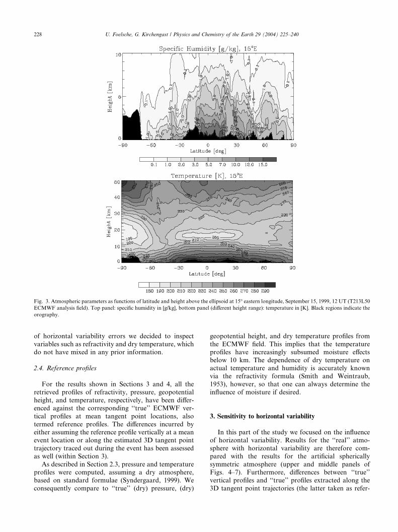
tical sampling. In order to illustrate the resolution of the
T213L50 field utilized, slices of specific humidity andtemperature are displayed in Fig. 3.
The MSIS climatological model (Hedin, 1991) was
used, with a smooth transition from the ECMWF
analysis field upwards, above the vertical domain of that
field. As we focused on the troposphere, we made the
reasonable assumption that ionospheric residual errors
can be neglected (Steiner et al., 1999). Forward model-
ing was therefore employed without ionosphere, whichcorresponds to considerable savings in computational
expenses.
We performed high-precision 3D ray tracing with
sub-millimetric accuracy and a sampling rate of 10 Hz
for all forward modeled events through the ECMWF
analysis. In order to be able to compare the ensemble
of measurements subjected to horizontal variability
with one without horizontal variability, two separate
ensembles of 60 events were forward modeled: one
with employing the analysis field with its 3D structure
as is, the other with artificially enforcing sphericalsymmetry for all events. The latter case was obtained
by applying the atmospheric profile at the mean tangent
point of an occultation event over the entire domain
probed.
As in the real atmosphere, occultation events over
oceans at low latitudes occasionally failed to penetrate
the lowest �4 km of the troposphere. In the present
simulations, the reason is that the ray tracer encounterssuper-refractive structures, which it cannot ‘‘overcome’’.
All 60 events included in the final ensemble and used for
computing the statistical results reached to a minimum
height of �2 km or closer to the surface. The retrieval
processing (Section 2.3) led, for individual events, to a
further increase of the minimum height reached.
2.3. Observation system modeling and retrieval processing
Realistic errors (including error sources like orbit
uncertainties, receiver noise, local multipath errors and
clock errors) have been superimposed on the obtained
simulated phase measurements. For this realistic
receiving system simulation, we reflected (conserva-
tively) the specifications and error characteristics of the
GRAS instrument (e.g., GRAS-SAG, 1998).Regarding retrieval processing, we applied a geo-
metric optics bending angle retrieval scheme, more
specifically, the ‘‘enhanced bending angle retrieval’’
algorithm of EGOPS. The core of this algorithm,
transforming phase delays to bending angles, is the
algorithm described by Syndergaard (1999), which was
enhanced to include inverse covariance weighted statis-
tical optimization (with prior best-fit a priori profilesearch) as described by Gobiet and Kirchengast (2002).
Since Forward Modeling has been performed without
ionosphere, ionospheric correction could be omitted.
Refractivity profiles have been computed using a
standard Abel transform retrieval employing the
EGOPS-internal algorithm of Syndergaard (1999).
Profiles of total atmospheric pressure and temperature,
respectively, have been obtained using a standard dry airretrieval algorithm as again developed by Syndergaard
(1999). Geopotential height profiles where obtained by
converting geometrical heights z of pressure levels via
the standard relation dZ ¼ ðgðz;uÞ=g0Þdz (e.g., Salby,
1996) to geopotential heights Z, where gðz;uÞ invokes
the international gravity formula (e.g., Kahle, 1984) and
g0 ¼ 9:80665 ms�2 is the standard acceleration of gra-
vity. We did not undertake to separately analyze tem-perature and humidity, since for this baseline analysis
Fig. 3. Atmospheric parameters as functions of latitude and height above the ellipsoid at 15� eastern longitude, September 15, 1999, 12 UT (T213L50
ECMWF analysis field). Top panel: specific humidity in [g/kg], bottom panel (different height range): temperature in [K]. Black regions indicate the
orography.
228 U. Foelsche, G. Kirchengast / Physics and Chemistry of the Earth 29 (2004) 225–240
of horizontal variability errors we decided to inspect
variables such as refractivity and dry temperature, which
do not have mixed in any prior information.
2.4. Reference profiles
For the results shown in Sections 3 and 4, all the
retrieved profiles of refractivity, pressure, geopotential
height, and temperature, respectively, have been differ-
enced against the corresponding ‘‘true’’ ECMWF ver-
tical profiles at mean tangent point locations, also
termed reference profiles. The differences incurred byeither assuming the reference profile vertically at a mean
event location or along the estimated 3D tangent point
trajectory traced out during the event has been assessed
as well (within Section 3).
As described in Section 2.3, pressure and temperature
profiles were computed, assuming a dry atmosphere,
based on standard formulae (Syndergaard, 1999). We
consequently compare to ‘‘true’’ (dry) pressure, (dry)
geopotential height, and dry temperature profiles from
the ECMWF field. This implies that the temperature
profiles have increasingly subsumed moisture effects
below 10 km. The dependence of dry temperature onactual temperature and humidity is accurately known
via the refractivity formula (Smith and Weintraub,
1953), however, so that one can always determine the
influence of moisture if desired.
3. Sensitivity to horizontal variability
In this part of the study we focused on the influence
of horizontal variability. Results for the ‘‘real’’ atmo-
sphere with horizontal variability are therefore com-
pared with the results for the artificial spherically
symmetric atmosphere (upper and middle panels of
Figs. 4–7). Furthermore, differences between ‘‘true’’
vertical profiles and ‘‘true’’ profiles extracted along the
3D tangent point trajectories (the latter taken as refer-
Fig. 4. Refractivity error statistics for the ensemble of all 60 occultation events in all sectors. Top panel: atmosphere with horizontal variability;
middle panel: atmosphere with spherical symmetry applied; bottom panel: vertical profile at mean tangent point minus profile along 3D tangent point
trajectory.
U. Foelsche, G. Kirchengast / Physics and Chemistry of the Earth 29 (2004) 225–240 229
ence) are shown (bottom panels of Figs. 4–7). The re-
sults for the full ensemble of 60 events are illustrated in
all panels. The gradual decrease in the number of events
towards lower tropospheric levels (small left-hand-side
Fig. 5. Pressure error statistics for the ensemble of all 60 occultation events in all sectors. Top panel: atmosphere with horizontal variability; middle
panel: atmosphere with spherical symmetry applied; bottom panel: vertical profile at mean tangent point minus profile along 3D tangent point
trajectory.
230 U. Foelsche, G. Kirchengast / Physics and Chemistry of the Earth 29 (2004) 225–240
subpanels) is due to the different minimum heights
reached by individual events.
Differencing of retrieved profiles with co-located
reference profiles allows computation of the total bias
errors and standard deviations in the parameters
under investigation. The exponential decrease of refrac-
tivity and pressure with height inhibits the visual
representation of absolute errors. Errors in refractivity
Fig. 6. Geopotential height error statistics for the ensemble of all 60 occultation events in all sectors. Top panel: atmosphere with horizontal
variability; middle panel: atmosphere with spherical symmetry applied; bottom panel: vertical profile at mean tangent point minus profile along 3D
tangent point trajectory.
U. Foelsche, G. Kirchengast / Physics and Chemistry of the Earth 29 (2004) 225–240 231
(Fig. 4) and pressure (Fig. 5) are thus shown as rel-
ative errors in units [%], while geopotential height(Fig. 6) and dry temperature errors (Fig. 7) are dis-
played in units [gpm] and [K], respectively. All sta-
tistics are shown between 1 km and 20 km above
(ellipsoidal) surface; dashed vertical lines mark rela-tive errors of 0.5% and absolute errors of 10 gpm and
1 K, respectively.
Fig. 7. Temperature error statistics for the ensemble of all 60 occultation events in all sectors. Top panel: atmosphere with horizontal variability;
middle panel: atmosphere with spherical symmetry applied; bottom panel: vertical profile at mean tangent point minus profile along 3D tangent point
trajectory.
232 U. Foelsche, G. Kirchengast / Physics and Chemistry of the Earth 29 (2004) 225–240
3.1. Refractivity errors
Fig. 4 illustrates that refractivity errors in a hori-zontally variable atmosphere increase considerably
below a height of about 7 km (top panel). In the
spherically symmetric atmosphere (middle panel), the
increase in refractivity error is significantly less pro-
nounced. Above 7 km, the error profiles are quitesmooth. There is a small negative bias of about
0.1%, standard deviations under horizontal variability
U. Foelsche, G. Kirchengast / Physics and Chemistry of the Earth 29 (2004) 225–240 233
(spherical symmetry) increase from �0.2% (<0.1%) at
20 km to �0.4% (�0.1%) at 7 km.
Below 7 km there is considerable structure in the
error profiles. In the spherically symmetric atmosphere,
standard deviations reach maximum values of 0.7% at
heights around 1.5 km, with a maximum (negative) bias
of 0.3%. In the realistic atmosphere, standard deviationsreach a maximum value of 1.8% at 1.8 km height, the
bias slightly exceeds 0.5% around 2.5 km and below 1.7
km.
3.2. Dependence on the geometry of reference profiles
According to Fig. 4 (bottom panel), differences be-
tween ‘‘true’’ vertical profiles at mean tangent pointlocations and ‘‘true’’ ones along actual 3D tangent point
trajectories are very small in the lower stratosphere,
since the EGOPS mean location estimate is designed to
fit best around 15 km. Below 7 km, however, the dif-
ferences are of a magnitude comparable to the errors
estimated under horizontal variability (top panel). This
implies that the geometrical mis-alignment of the actual
tangent point trajectory with the mean-vertical con-tributes as a major source to horizontal variability error.
Additional visual evidence for this is that the bias below
7 km in the lower panel appears roughly mirror-
symmetric relative to the one in the upper panel. This
occurs since the geometrical mis-alignment is a main
bias source in both cases so that a clearly visible effect
left is the change in sign due to the upper panel using the
mean-vertical profile as reference while the lower paneluses the along-trajectory one.
This finding applies also to the other parameters
(Figs. 5–7) and indicates the importance of utilizing
tropospheric RO profiles not just vertically but as good
as possible consistent with the actual tangent point
trajectory (or, more generally, occultation plane move-
ment). Overall, the results show that the performance in
the realistic horizontally variable troposphere is mark-edly improved if measured against the actual tangent
point trajectory.
3.3. Pressure errors
The pressure errors (Fig. 5) display a similar behavior
as the refractivity errors, though the smaller-vertical-
scale variations are less pronounced due to the hydro-static integration.
In the spherical symmetry case, all relative errors
increase with decreasing height (bias from 0.1% to
0.2%, standard deviation from 0.2% to 0.34%). In the
realistic atmosphere with horizontal variability, stan-
dard deviations are smallest around 13 km height
(0.2%), below they increase up to �0.5% around 1.3
km height, where the negative bias also has its maxi-mum value of �0.2%.
3.4. Geopotential height errors
Errors in the geopotential height of pressure surfaces
are shown in Fig. 6 as function of pressure height zp (a
convenient pressure coordinate defined as zp ¼ �7 � lnp [hPa]/1013.25), which is closely aligned with height z).Mirroring the pressure errors (see, e.g., Syndergaard,1999, on the relation between pressure and geopotential
height), positive biases in geopotential height corre-
spond to negative biases in pressure (cf. Figs. 5 and 6).
In the realistic atmosphere, biases are <5 gpm above
about 7 km, exceed 10 gpm below about 3 km, and
reach a maximum of �13 gpm at �1.3 km pressure
height (corresponding to a pressure error of �0.2%).
Standard deviations are <15 gpm above about 5 km andreach �33 gpm at lowest levels. In the spherically sym-
metric atmosphere, the bias above about 7 km is largely
the same as in the realistic case, but remains <8 gpm
lower down (compared to �13 gpm with horizontal
variability); the standard deviation reaches �20 gpm
(instead of �33 gpm) at lowest levels.
3.5. Temperature errors
The dry temperature errors are depicted in Fig. 7. In
the scenario with horizontal variability, all errors below
7 km are larger than the corresponding errors under
spherical symmetry. A positive bias of �1 K is reached
around 2.6, 1.5, and 1.2 km, respectively, where stan-
dard deviations of about 4 K are encountered.
Under spherical symmetry, the maximum bias is 0.4K at 1.2 km, standard deviations remain smaller than
1.2 K. Between 7 and 20 km there is essentially no
temperature bias in both scenarios (i.e., always smaller
than 0.1 K).
4. Sensitivity to the angle-of-incidence
In this part of the study, the sensitivity of retrieval
products to the angle-of-incidence of occultation rays
relative to the boresight direction of the receiving an-
tenna (aligned with the LEO orbit plane) is analyzed.
Error analyses have been performed for each azimuth
sector (ensembles of 20 events), for every atmospheric
parameter under study. Occultation events in the 0–10�sector are associated with almost co-planar GNSS andLEO satellites, which should lead to the most-vertical
and best-quality occultation events.
Errors in refractivity and pressure, respectively, are––
as in Section 3––displayed as relative values in units [%],
geopotential height and dry temperature errors as
absolute values in units [gpm] and [K], respectively. All
statistics are shown between 1 and 20 km above the
(ellipsoidal) surface; the dashed vertical lines indicate
234 U. Foelsche, G. Kirchengast / Physics and Chemistry of the Earth 29 (2004) 225–240
relative errors of 0.5% and absolute errors of 10 gpm
and 1 K, respectively.
Each of the following figures, Figs. 8–11, shows the
results for sector 1 in the top panel, for sector 2 in the
Fig. 8. Refractivity error statistics for occultation events in sector 1 (top p
middle panel, and for sector 3 in the bottom panel,
respectively (the three sectors are defined as described in
Section 2.1). Refractivity errors are shown in Fig. 8,
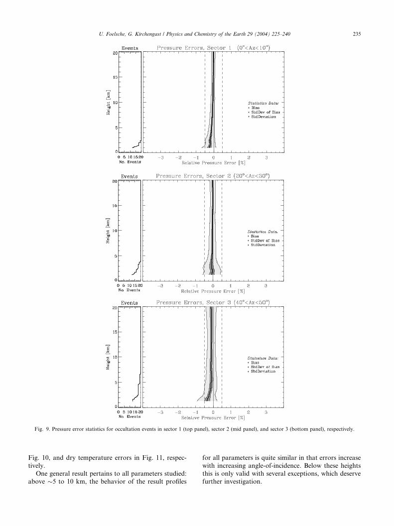
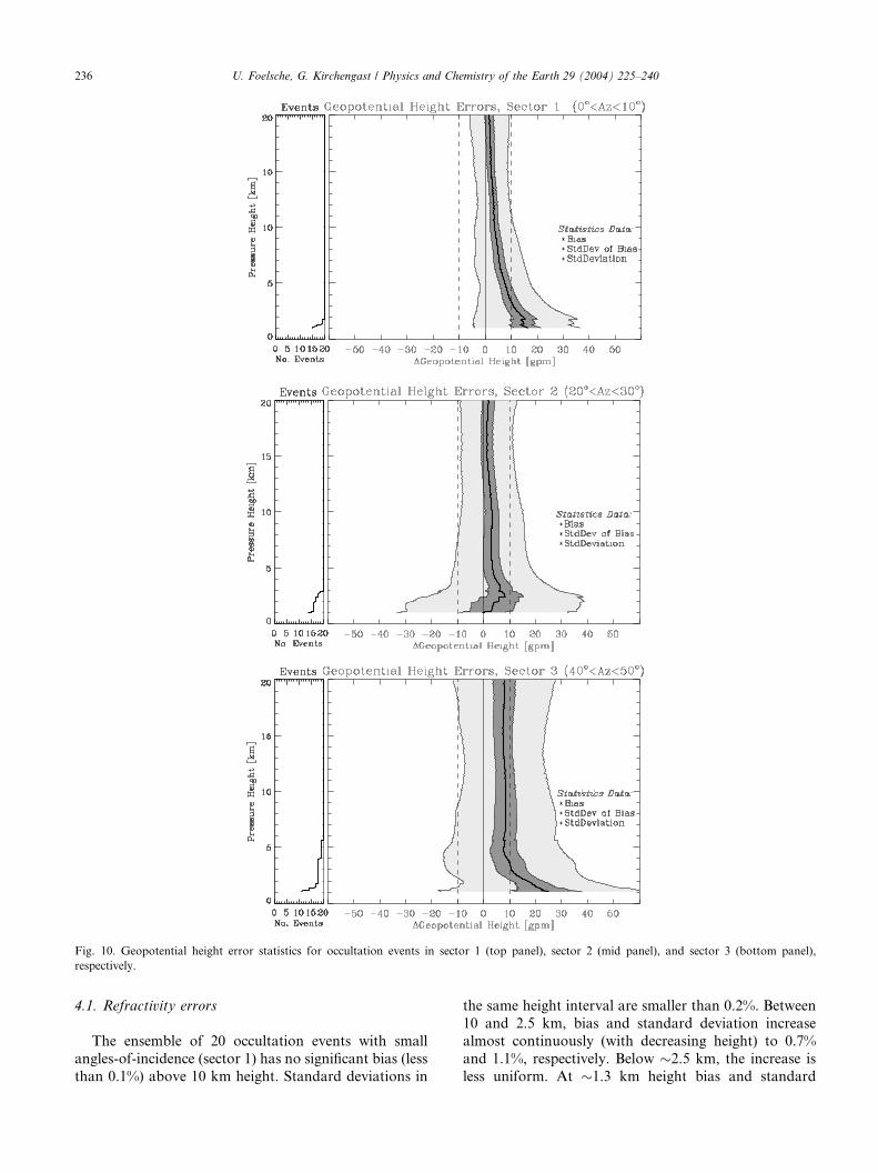
pressure errors in Fig. 9, geopotential height errors in