Sensitivity of the climate system to small

perturbations of external forcing

V.P. Dymnikov, E.M. Volodin, V.Ya. Galin, A.S. Gritsoun, A.V. Glazunov, N.A. Diansky, V.N. Lykosov

Institute of Numerical Mathematics RAS, Moscow

• The climate system - the system consisting of atmosphere, hydrosphere, cryosphere, land and biota.

• The climate - the ensemble of states the climate system passes through during a sufficiently long time interval.

• Characteristics of the climate system as a physical object:

• quasi-two-dimensionality

• impossibility of purposeful physical experiments

The central direction of the climate sensitivity studies:

mathematical modeling

Problems:

1. The identification of models by sensitivity.

2. Is it possible to determine the sensitivity of the climate

system to small external forcing using single trajectory?

The climate model sensitivity to the increasing of CO2

CMIP - Coupled Model Intercomparison Project

http://www-pcmdi.llnl.gov/cmip

CMIP collects output from global coupled ocean-atmosphere general circulation models (about 30 coupled GCMs). Among other usage, such models are employed both to detect anthropogenic effects in the climate record of the past century and to project future climatic changes due to human production of greenhouse gases and aerosols.

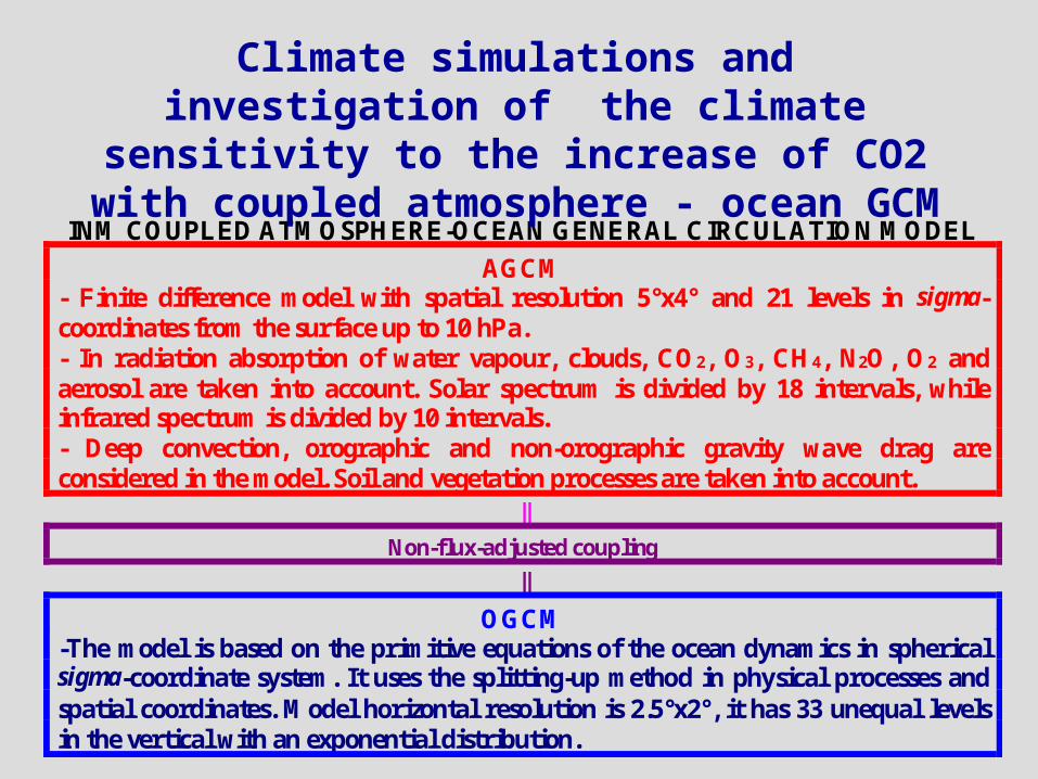
INM COUPLED ATMOSPHERE-OCEAN GENERAL CIRCULATION MODEL

AGCM- Finite difference model with spatial resolution 5°x4° and 21 levels in sigma-coordinates from the surface up to 10 hPa.- In radiation absorption of water vapour, clouds, CO2, O3, CH4, N2O, O2 andaerosol are taken into account. Solar spectrum is divided by 18 intervals, whileinfrared spectrum is divided by 10 intervals.- Deep convection, orographic and non-orographic gravity wave drag areconsidered in the model. Soil and vegetation processes are taken into account.

||

Non-flux-adjusted coupling

||

OGCM-The model is based on the primitive equations of the ocean dynamics in sphericalsigma-coordinate system. It uses the splitting-up method in physical processes andspatial coordinates. Model horizontal resolution is 2.5°x2°, it has 33 unequal levelsin the vertical with an exponential distribution.

Climate simulations and investigation of the climate sensitivity to the increase of CO2 with

coupled atmosphere - ocean GCM

Response to the increasing of CO2CMIP models (averaged)

INM model

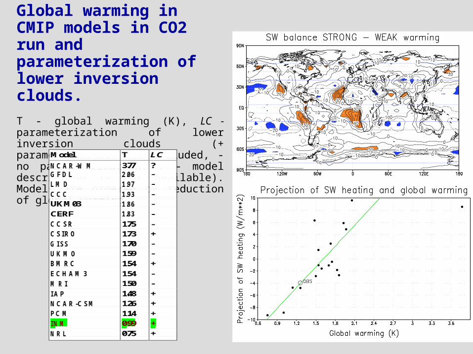
Global warming in CMIP models in CO2 run and parameterization of lower inversion clouds.

T - global warming (K), LC - parameterization of lower inversion clouds (+ parameterization was included, - no parameterization, ? - model description is not available). Models are ordered by reduction of global warming.

1. Formulation of model equations

2. Proof of the existence and uniqueness theorems

3. Attractor existence theorem, dimension estimate

4. Stability of the attractor (as set) and measure on it

5. Finite-dimensional approximations and correspondent

convergence theorems

),,( tuFdtdu

Mathematical theory of climate

Mathematical theory of climate(sensitivity)

6. Construction of the response operator for measure and its moments

(“optimal perturbation”, inverse problems,….)

7. Methods of approximation for

8. Numerical experiments

fMu

M

Response operator for 1st moment (linear theory)

Linear model for the low-frequency variability of the original system:

( A is stable, is white noise in time)

Perturbed system

)(tAudtdu

ftuAdtud

)(

)(t

Stationary response

For covariance matrix we have

and response operator M could be obtained as

fMfAu

uuu

1

)0()exp()( CAC

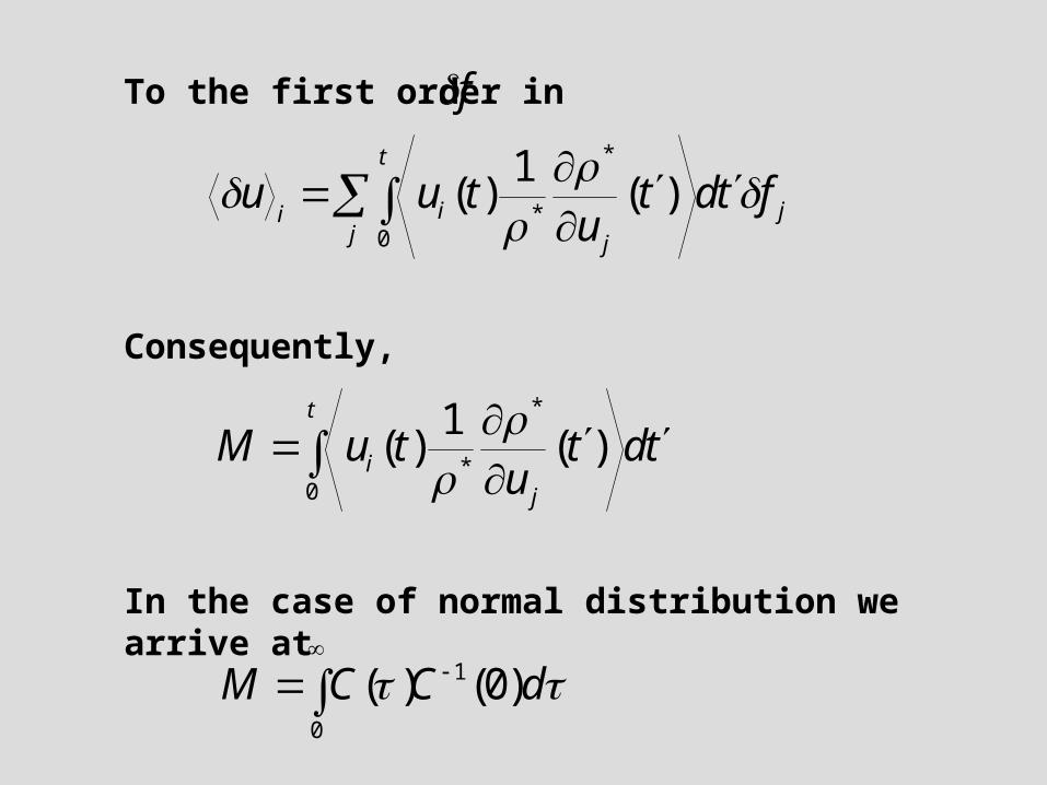
dCCM )0()( 1

0

Response operator for 1st moment (nonlinear theory)

Nonlinear model for system dynamics:

( is the white noise in time)

Perturbed system

)()( tuBdtdu

ftuBdtud

)()(

)(t

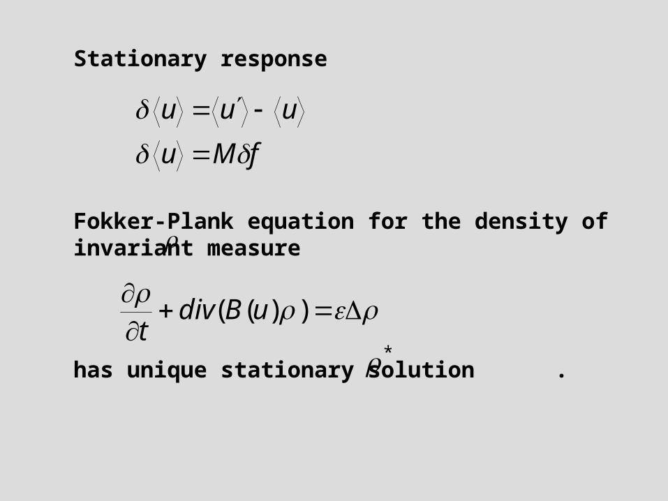
Stationary response

Fokker-Plank equation for the density of invariant measure

has unique stationary solution .

fMu

uuu

))(( uBdivt

*

To the first order in

Consequently,

In the case of normal distribution we arrive at

jj

t

j

iiftdt

utuu

0

*

*)(

1)(

tdtu

tuMt

j

i

0

*

*)(

1)(

dCCM )0()( 1

0

f

CCM0 (E.J.Pitcher et.al., J.Atmos.Sci., (1982), v.40., p.580)

1) 9 levels in -coordiante

2) prognostic variables: horizontal velocity divergence, vertical component of the relative

vorticity, temperature, relative humidity, surface pressure

3) Parameterizations of convection, condensation, latent and explicit heat fluxes, radiation,

vertical and horizontal diffusion

4) Galerkin method for space approximation. Basis functions - spherical harmonics, R15

truncation. Phase space dimension - 18352

Numerical experiments

Construction of the approximate response operator (A.S.Gritsoun,G.Branstator, V.P.Dymnikov, R.J.Numer.Analysis&M.Model, (2002), v.17,p. 399)

CCM0 (right) and M-operator (left) responses to the “sinusoidal” heating anomaly at (60E, 00N). First row – at σ=0.336, second row - at σ=0.811

Reconstruction of the CCM0 response to the sinusoidal heating anomaly

336811336T

811T

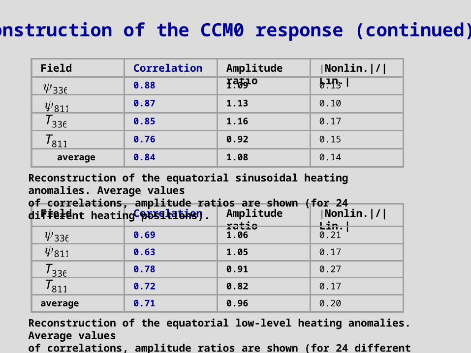
Field Correlation Amplitude ratio |Nonlin.|/|Lin.|

0.88 1.09 0.13

0.87 1.13 0.10

0.85 1.16 0.17

0.76 0.92 0.15

average 0.84 1.08 0.14

336811

336T

811T

Field Correlation Amplitude ratio |Nonlin.|/|Lin.|

0.69 1.06 0.21

0.63 1.05 0.17

0.78 0.91 0.27

0.72 0.82 0.17

average 0.71 0.96 0.20

Reconstruction of the equatorial low-level heating anomalies. Average valuesof correlations, amplitude ratios are shown (for 24 different heating positions).

Reconstruction of the equatorial sinusoidal heating anomalies. Average valuesof correlations, amplitude ratios are shown (for 24 different heating positions).

Reconstruction of the CCM0 response (continued)

Reconstruction of the low-level heating anomalies using

the inverse response operator

Real heating anomalies at σ=0.991 ( in K/day) are shown on the left, reconstructedones - on the right. Positions of the anomalies are (30E,40N) and (45E,40N).

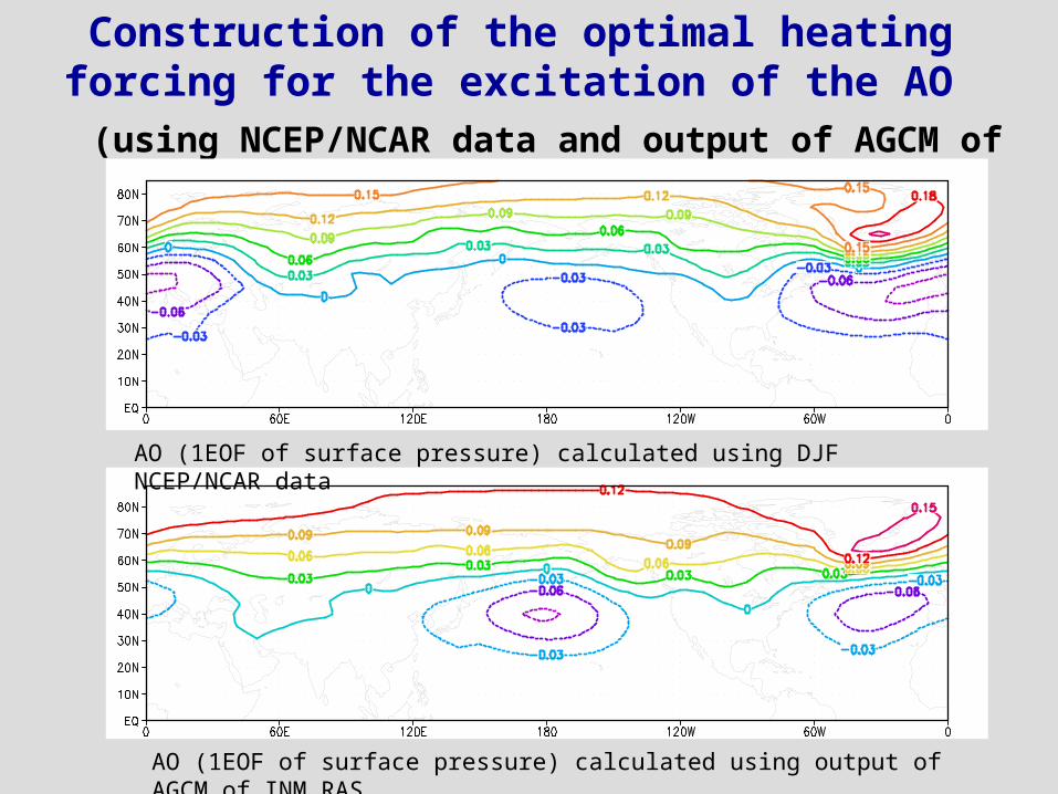
Construction of the optimal heating forcing for the excitation of the AO

(using NCEP/NCAR data and output of AGCM of INM RAS)

AO (1EOF of surface pressure) calculated using DJF NCEP/NCAR data

AO (1EOF of surface pressure) calculated using output of AGCM of INM RAS

Procedure for the construction of the approximate response operator is analogues to (A.S.Gritsoun, G.Branstator, V.P.Dymnikov, R.J.Numer. Analysis&M.Model, (2002), v.17,p. 399)

Optimal perturbation for AO (1EOF of PS)calculated using NCEP/NCAR reanalysis data(zonal average)

Optimal perturbation for AO (1EOF of PS)calculated using output of AGCM of INM RAS(zonal average)

Global warming in CMIP models in CO2 run and parameterization of lower inversion clouds.

T - global warming (K), LC - parameterization of lower inversion clouds (+ parameterization was included, - no parameterization, ? - model description is not available). Models are ordered by reduction of global warming.

Acknowledgments

Our studies are supported by:

• Russian Ministry for Industry, Sciences and Technology

•Russian Academy of Sciences

• Russian Foundation for Basic Research

• INTAS