Sensor Network for Real-time In-situ Seismic Tomography

Lei Shi, Wen-Zhan Song, Fan Dong and Goutham KamathGeorgia State University, Atlanta, Georgia, U.S.A.

Keywords: Sensor Networks, Design, In-network Processing and Seismic Tomography.

Abstract: Most existing seismic exploration or volcano monitoring systems employ expensive broadband seismometeras instrumentation. At present raw seismic data are typically collected at central observatories for post process-ing. With a high-fidelity sampling, it is virtually impossible to collect raw, real-time data from a large-scaledense sensor network due to severe limitations of energy and bandwidth at current, battery-powered sensornodes. At some most threatening and active volcanoes, only tens of nodes are maintained. With a smallnetwork and post processing mechanism, existing system do not yet have the capability to recover physicaldynamics with sufficient resolution in real-time. This limits our ability to understand earthquake zone or vol-cano dynamics. To obtain the seismic tomography in real-time and high resolution, a new sensor networksystem for real-time in-situ seismic tomography computation is proposed in this paper. The design of the sen-sor network consists of hardware, sensing and data processing components for automatic arrivaltime pickingand tomography computation. This system design is evaluated both in lab environment for 3D tomographywith real seismic data set and in outdoor field test for 2D surface tomography.

1 INTRODUCTION

In present, most existing seismic exploration or vol-cano monitoring systems use expensive broadbandseismometer and collect raw seismic data for postprocessing. Seismic sampling rates for seismic ex-ploration are usually in the range of 16-24 bit at 50-200Hz. Collecting all the raw data in real-time froma large-scale dense sensor network is virtually impos-sible due to severe limitations of energy and band-width at current, battery-powered sensor nodes. Asa result, at some most threatening, active volcanoes,fewer than 20 nodes (Song et al., 2009) are thus main-tained. With such a small network and post process-ing mechanism, existing system do not yet have thecapability to recover physical dynamics with suffi-cient resolution in real-time. This limits our abilityto understand earthquake zone or volcano dynamicsand physical processes under ground or inside vol-cano conduit systems. Substantial scientific discov-eries on the geology and physics of earthquake zoneand active volcanism would be imminent if the seis-mic tomography inversion could be in real-time andthe resolution could be increased by an order of mag-nitude or more. This requires a large-scale networkwith automatic in-network processing and computa-tion capability.

To date, the sensor network technology has ma-

tured to the point where it is possible to deploy andmaintain a large-scale network for volcano monitor-ing and utilize the computing power of each node forsignal processing to avoid raw seismic data collectionand support tomography inversion in real-time. Themethods commonly used today in the procedure ofseismic tomography computation cannot be directlyemployed under field circumstances proposed herebecause they rely on expensive broadband stationsand post processing, also require massive amountsof raw seismic data collected on a central process-ing unit. Thus, real-time seismic tomography of highresolution requires a new mechanism with respectto low-cost energy efficient system design and in-network information processing. Then it is possible todeploy a large-scale network for long-term and com-pute the tomography in real-time. To clearly addressthe challenges in this paper, we first give a short de-scription on the background knowledge of seismic to-mography based on traveltime principle.

The first-arrival traveltime tomography uses P-wave first arrival times at sensor nodes to derive theinternal velocity structure of the subsurface. The ba-sic workflow of traveltime tomography illustrated inFigure 1 involves four steps: (a) P-wave Arrival TimePicking. Once an earthquake event happens, the sen-sor nodes that detect seismic disturbances record thesignals. The P-wave arrival times need to be extracted

118Shi, L., Song, W-Z., Dong, F. and Kamath, G.Sensor Network for Real-time In-situ Seismic Tomography.DOI: 10.5220/0005897501180128In Proceedings of the International Conference on Internet of Things and Big Data (IoTBD 2016), pages 118-128ISBN: 978-989-758-183-0Copyright c© 2016 by SCITEPRESS – Science and Technology Publications, Lda. All rights reserved

Event Location Ray Tracing Tomography Inversion

Sensor Node

Seismic Rays

Estimated Magma Area

Blocks on Ray PathMagma

Estimated Event Location

Earthquake Event

(b) (c) (d)

P-wave Arrival Time Picking

P-wave

(a)

Figure 1: Workflow of first-arrival traveltime tomography.

from the raw seismic data; (b) Event Location. TheP-wave arrival times and locations of sensor nodesare used to estimate the event hypocenter and origintime in the volcanic edifice; (c) Ray Tracing. Follow-ing each event, seismic rays propagate to nodes andpass through anomalous media. These rays are per-turbed and thus register anomalous residuals. Giventhe source locations of the seismic events and currentvelocity model, ray tracing is to find the ray pathsfrom the event hypocenters to the nodes; (d) Tomog-raphy Inversion. The traced ray paths, in turn, areused to image a tomography model of the velocitystructure. As shown in Figure 1 the volcano is parti-tioned into small blocks and the seismic tomographyproblem can be formulated as a large and sparse ma-trix inversion problem.

In traditional seismology, the raw seismic data iscollected for manual analysis including P-wave ar-rival time picking on the seismograms. Then cen-tralized methods will process the data and computeseismic tomography. Keep in mind that our goal isto design a system which can deliver tomography inreal-time over a large-scale senor network by utilizingthe limited communication ability in the network andthe computation power on the sensor node. To reachthis goal, no raw seismic data should be transmittedover the network, which requires a light weighted al-gorithm that can accurately pick the P-wave arrivaltime on the sensor nodes locally inside the network.

This paper presents a sensor network system forreal-time in-situ seismic tomography computation.The design of the sensor network consists of hard-ware, sensing, data processing, algorithm for auto-matic arrivaltime picking and so on. This system de-sign is evaluated both in lab environment for 3D to-mography with real seismic data set (previous deploy-ment on San Andreas Fault (SAF) in Parkfield) and inoutdoor field test for 2D surface tomography.

The rest of the paper is organized as follows. Sec-tion 2 shows the system architecture and discusses thesystem design in details. In section 3, we evaluate thesignal quality compared with a industry level com-mercial data logger for seismology and validate thearrival time picking algorithm with both field test andreal seismic data set. Section 4 describes the eval-

uation of the system both in lab environment and inoutdoor field test. Section 5 discusses related work.Section 6 concludes this paper and outlines the futurework.

2 SYSTEM DESIGN

In this section, we give the overview of our system ar-chitecture and the details of both hardware and soft-ware design. According to the motivation and require-ment of the system design discussed above, the spe-cific goals of the sensor network system design is asfollowing:• Synchronized Sampling. The event location and

travel-time tomography requires the P-wave ar-rival time of earthquake events. The P-wave ar-rival time analysis is based on the temporal andspacial correlation of the recorded signals on sta-tions. So all stations need to perform synchro-nized sampling and timestamp the record withprecise UTC time. The synchronization accuracyshould be less than the time interval of sampling(e.g. 20 millisecond for 50Hz sampling rate).

• Long-term Robust Deployment. To get accurateevent location and high resolution seismic tomog-raphy, the more data recorded the better result canbe potentially delivered. Since the earthquake ac-tivities are unpredictable, the long-term robust de-ployment is necessary to get enough data. Also,due to the harsh weather conditions for remote de-ployment, a low-cost energy efficient station withrenewable energy and weatherproof capacity is re-quired.

• P-wave Arrival Time Picking. As we discussed insection 1, this sensor network system will send thearrival time back instead of all raw seismic data.The system must be able to continuously moni-tor the signal, detect and pick arrival time in real-time.

• Online Monitoring and Configuration. To mon-itor the status of the network, perform the real-time signal processing and in-situ computation,the sensor network should be able to respond to

Sensor Network for Real-time In-situ Seismic Tomography

119

external control from the base station for statusreport or node configuration. The command andcontrol needs to be delivered reliably in real-time.

• Distributed Computation Extension. This systemis not limited to be a in-situ signal processingand data collection framework. In the future, thesystem can be used for more complicated seis-mic analysis that may include cross correlation ofsignals between stations, distributed computationand so on. Those tasks will require more compu-tation power on each sensor node. An extensionfor adding a computation unit is required to makethis system more extensive and general.

2.1 System Architecture

Our system consists of several components. Figure 2shows the architecture of the sensor network systemdesign. First, the sensor nodes with seismometers andRF modules form a mesh network. Each sensor con-tinuously records the signal, once an event happened,the sensor will detect it and pick the P-wave arrivaltime from the signals. Then the arrival time alongwith the station coordinates is delivered to the basestation. The base station is a computer that equippedwith RF module, it runs various tools to process thereceived data, compute the tomography, visualize theresult, monitor the network status and configure thesensor nodes. This system can deliver either 3D to-mography through event location, ray tracing and in-version, or 2D surface tomography with Eikonal to-mography method (Lin et al., 2009).

Base Station

EventLocation

RayTracing

3DTomography

TomographyGUI

EikonalTomography

Monitoring & Configuration

GUI

Arrival times

Status andResponds

Command andRequest

Sensor nodes each equipped withseismometer and RF module

Figure 2: Sensor Network System Architecture.

2.2 Hardware Design

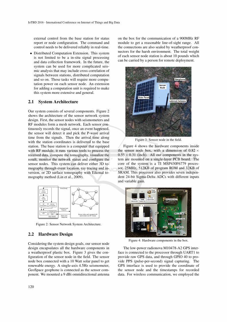
Considering the system design goals, our sensor nodedesign encapsulates all the hardware components ina weatherproof plastic box. Figure 3 gives the con-figuration of the sensor node in the field. The sensornode box connected with a 10 Watt solar panel to getrenewable energy. A single-axis 4.5Hz seismometer,GeoSpace geophone is connected as the sensor com-ponent. We mounted a 9 dBi omnidirectional antenna

on the box for the communication of a 900MHz RFmodule to get a reasonable line-of-sight range. Allthe connections are also sealed by weatherproof con-nectors for the harsh environment. The total weightof each sensor node station is about 10 pounds whichcan be carried by a person for remote deployment.

Figure 3: Sensor node in the field.

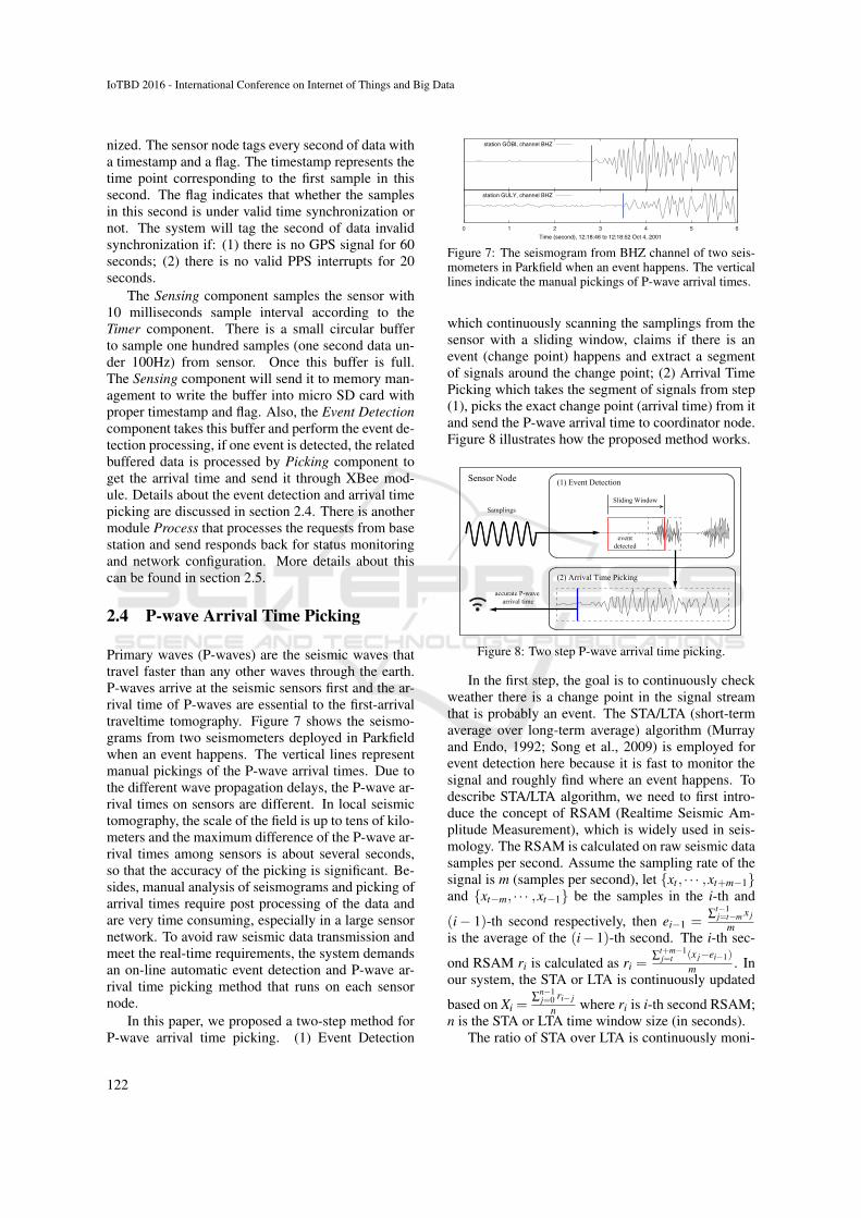
Figure 4 shows the hardware components insidethe sensor node box, with a dimension of 0.82×0.55× 0.31 (inch). All our components in the sys-tem are mounted on a single-layer PCB board. Thecore of the system is a TI MSP430F6779 proces-sor, 25MHz, 512KB of program ROM and 32KB ofSRAM. This processor also provides seven indepen-dent 24-bit Sigma-Delta ADCs with different inputsand variable gain.

Figure 4: Hardware components in the box.

The low-power radionova M10478-A2 GPS inter-face is connected to the processor through UART1 toprovide raw GPS data, and through GPIO 40 to pro-vide PPS (pulse-per-second) signal capturing. TheGPS interface is used to provide the coordinate ofthe sensor node and the timestamps for recordeddata. For wireless communication, we employed the

IoTBD 2016 - International Conference on Internet of Things and Big Data

120

XBee-PRO 900HP module to provide a low-power,low maintenance, long outdoor range and self orga-nized wireless network. XBee module takes advan-tage of the DigiMesh networking protocol. It can runon dense network operation and support for sleepingrouters for energy efficient. Besides, various point-to-multipoint configurations are available for the net-work. The MSP430 is connected to XBee usingUART2 with 9600 baud that provides 960 Kbps datarate.

MSP430F6779

UART1 GPIO40 UART2

GPS

TX RX PPS

XBee

TX RX

RX TX

External antenna

Sensor

CH3 CH2 CH1

ADC0 ADC1 ADC2

RX TX

micro SD card BeagleBone Black

SPI0 GPIO68 SPI1 GPI

O72

GPI

O70

SOM

I

SIM

O

SCLK

SPIS

C

SOM

I

SIM

O

SCLK

SPIS

C

EN

Figure 5: The main hardware components connection.

Since the sensor network is designed to sense thesignal, pick and send the P-wave arrival timestampback without transmitting the raw seismic data. Allthe raw data is stored in a micro SD card for otherpost analysis required by seismologists. We use theDM3D-SF connector and connect the processor withmemory card through SPI0 for SPI communicationand clock, and through GPIO 68 for SPI card selectpin. The node sensor connector is designed to con-nect up to three channels of seismometer. The nodecan connect either to a single-axis or a tri-axis geo-phone. Both geophones are passive instruments andthe ground motion can generate voltage which is dig-itized by the ADC module in MSP430.

For the distributed computation extension require-ment, one BeagleBone Black (BBB) module is con-nected with the expansion connector to the boardthrough its SPI0 interface. We use the SPI1 onMSP430 for SPI communication and clock, the GPIO72 for SPI card select pin and the GPIO 70 as thepower switch for BBB. The main hardware compo-nents connection relationships are shown in Figure 5.

2.3 Sensing and Data Processing

Aim to achieve the system design goals, based on ourhardware design, we give the description of the soft-ware design for sensing and data processing on thesensor node in this section. Figure 6 illustrates theframework of the sensing and data processing com-ponents on the sensor node.

Sensing

Memory Management

SD Card

GPSParse

EventDetection

Timer

GPS Valid

Raw Data

Sensor XBee RTCGPS

Read Write

Buffer full

Picking

Picking Buffer

Process PPS

Arrvial times

RequestResponds

Figure 6: Sensing and Data Processing Framework.

Since the accurate event location and high-resolution tomography are depend on precise timingby utilizing the temporal and spacial correlation ofrecorded signals across stations. The first goal of oursystem design is synchronized sampling and preciseUTC time timestamp for the recorded data. Our col-laborators from seismology requires 100Hz samplingrate on our open nodes. Notice that, the synchronizedsampling is based on time synchronization but not thesame. Synchronized sampling does not only meansthat all sensor nodes in the network has the same sam-ple interval but also sample at the same time point.

In the hardware design, each sensor node employsa low-cost GPS receiver that provides UTC time in-formation and PPS signal. The GPS system time fromGPS signal has an accuracy within 50ns referencedto UTC time, it can be used for time synchroniza-tion. The problem is that decoding and processingof the GPS message can generate delays and degradethe synchronization accuracy. Instead, we use PPSsignals to synchronize the RTC. To achieve the syn-chronized sampling, we designed a Timer componentto maintain RTC with millisecond resolution. Thenwhen the system catches the first valid PPS interrupt,the timer is reset and keep counting on milliseconds.When next valid PPS interrupt is captured, if the timeris not in exact thousand milliseconds, the timer will bereset and the RTC will be synchronized properly.

Notice that, the GPS signal can disappear or thePPS signal can not fire properly. If the time periodwithout GPS signal or valid PPS signals is long, thesampling across sensor nodes might not be synchro-

Sensor Network for Real-time In-situ Seismic Tomography

121

nized. The sensor node tags every second of data witha timestamp and a flag. The timestamp represents thetime point corresponding to the first sample in thissecond. The flag indicates that whether the samplesin this second is under valid time synchronization ornot. The system will tag the second of data invalidsynchronization if: (1) there is no GPS signal for 60seconds; (2) there is no valid PPS interrupts for 20seconds.

The Sensing component samples the sensor with10 milliseconds sample interval according to theTimer component. There is a small circular bufferto sample one hundred samples (one second data un-der 100Hz) from sensor. Once this buffer is full.The Sensing component will send it to memory man-agement to write the buffer into micro SD card withproper timestamp and flag. Also, the Event Detectioncomponent takes this buffer and perform the event de-tection processing, if one event is detected, the relatedbuffered data is processed by Picking component toget the arrival time and send it through XBee mod-ule. Details about the event detection and arrival timepicking are discussed in section 2.4. There is anothermodule Process that processes the requests from basestation and send responds back for status monitoringand network configuration. More details about thiscan be found in section 2.5.

2.4 P-wave Arrival Time Picking

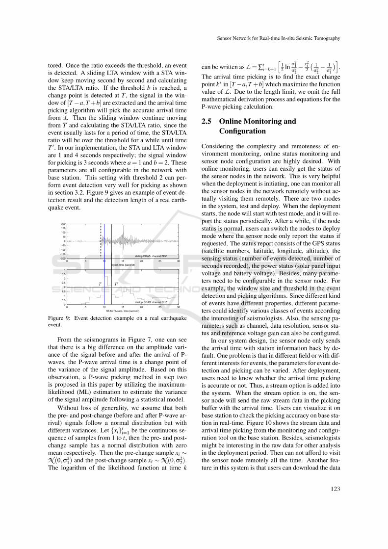
Primary waves (P-waves) are the seismic waves thattravel faster than any other waves through the earth.P-waves arrive at the seismic sensors first and the ar-rival time of P-waves are essential to the first-arrivaltraveltime tomography. Figure 7 shows the seismo-grams from two seismometers deployed in Parkfieldwhen an event happens. The vertical lines representmanual pickings of the P-wave arrival times. Due tothe different wave propagation delays, the P-wave ar-rival times on sensors are different. In local seismictomography, the scale of the field is up to tens of kilo-meters and the maximum difference of the P-wave ar-rival times among sensors is about several seconds,so that the accuracy of the picking is significant. Be-sides, manual analysis of seismograms and picking ofarrival times require post processing of the data andare very time consuming, especially in a large sensornetwork. To avoid raw seismic data transmission andmeet the real-time requirements, the system demandsan on-line automatic event detection and P-wave ar-rival time picking method that runs on each sensornode.

In this paper, we proposed a two-step method forP-wave arrival time picking. (1) Event Detection

station GOBI, channel BHZ

0 1 2 3 4 5 6Time (second), 12:18:46 to 12:18:52 Oct 4, 2001

station GULY, channel BHZ

Figure 7: The seismogram from BHZ channel of two seis-mometers in Parkfield when an event happens. The verticallines indicate the manual pickings of P-wave arrival times.

which continuously scanning the samplings from thesensor with a sliding window, claims if there is anevent (change point) happens and extract a segmentof signals around the change point; (2) Arrival TimePicking which takes the segment of signals from step(1), picks the exact change point (arrival time) from itand send the P-wave arrival time to coordinator node.Figure 8 illustrates how the proposed method works.

(1) Event DetectionSensor Node

Sliding Window

(2) Arrival Time Picking

eventdetected

accurate P-wave arrival time

Samplings

Figure 8: Two step P-wave arrival time picking.

In the first step, the goal is to continuously checkweather there is a change point in the signal streamthat is probably an event. The STA/LTA (short-termaverage over long-term average) algorithm (Murrayand Endo, 1992; Song et al., 2009) is employed forevent detection here because it is fast to monitor thesignal and roughly find where an event happens. Todescribe STA/LTA algorithm, we need to first intro-duce the concept of RSAM (Realtime Seismic Am-plitude Measurement), which is widely used in seis-mology. The RSAM is calculated on raw seismic datasamples per second. Assume the sampling rate of thesignal is m (samples per second), let {xt , · · · ,xt+m−1}and {xt−m, · · · ,xt−1} be the samples in the i-th and

(i− 1)-th second respectively, then ei−1 =∑t−1

j=t−m x j

mis the average of the (i− 1)-th second. The i-th sec-

ond RSAM ri is calculated as ri =∑t+m−1

j=t (x j−ei−1)

m . Inour system, the STA or LTA is continuously updated

based on Xi =∑n−1

j=0 ri− j

n where ri is i-th second RSAM;n is the STA or LTA time window size (in seconds).

The ratio of STA over LTA is continuously moni-

IoTBD 2016 - International Conference on Internet of Things and Big Data

122

tored. Once the ratio exceeds the threshold, an eventis detected. A sliding LTA window with a STA win-dow keep moving second by second and calculatingthe STA/LTA ratio. If the threshold b is reached, achange point is detected at T , the signal in the win-dow of [T−a,T +b] are extracted and the arrival timepicking algorithm will pick the accurate arrival timefrom it. Then the sliding window continue movingfrom T and calculating the STA/LTA ratio, since theevent usually lasts for a period of time, the STA/LTAratio will be over the threshold for a while until timeT ′. In our implementation, the STA and LTA windoware 1 and 4 seconds respectively; the signal windowfor picking is 3 seconds where a = 1 and b = 2. Theseparameters are all configurable in the network withbase station. This setting with threshold 2 can per-form event detection very well for picking as shownin section 3.2. Figure 9 gives an example of event de-tection result and the detection length of a real earth-quake event.

-200-150-100-50

0 50

100 150 200

0 5 10 15 20 25 30Signal, time (second)

station CGAS, channel BHZ

0 0.5

1 1.5

2 2.5

3 3.5

4

0 5 10 15 20 25 30STA/LTA ratio, time (second)

station CGAS, channel BHZ

T T’

Figure 9: Event detection example on a real earthquakeevent.

From the seismograms in Figure 7, one can seethat there is a big difference on the amplitude vari-ance of the signal before and after the arrival of P-waves, the P-wave arrival time is a change point ofthe variance of the signal amplitude. Based on thisobservation, a P-wave picking method in step twois proposed in this paper by utilizing the maximum-likelihood (ML) estimation to estimate the varianceof the signal amplitude following a statistical model.

Without loss of generality, we assume that boththe pre- and post-change (before and after P-wave ar-rival) signals follow a normal distribution but withdifferent variances. Let {xi}t

i=1 be the continuous se-quence of samples from 1 to t, then the pre- and post-change sample has a normal distribution with zeromean respectively. Then the pre-change sample xi ∼N (0,σ2

1) and the post-change sample xi ∼ N (0,σ22).

The logarithm of the likelihood function at time k

can be written as L =∑ti=k+1

[12 ln σ2

1σ2

2− x2

i2

( 1σ2

2− 1

σ21

)].

The arrival time picking is to find the exact changepoint k∗ in [T−a,T +b] which maximize the functionvalue of L . Due to the length limit, we omit the fullmathematical derivation process and equations for theP-wave picking calculation.

2.5 Online Monitoring andConfiguration

Considering the complexity and remoteness of en-vironment monitoring, online status monitoring andsensor node configuration are highly desired. Withonline monitoring, users can easily get the status ofthe sensor nodes in the network. This is very helpfulwhen the deployment is initiating, one can monitor allthe sensor nodes in the network remotely without ac-tually visiting them remotely. There are two modesin the system, test and deploy. When the deploymentstarts, the node will start with test mode, and it will re-port the status periodically. After a while, if the nodestatus is normal, users can switch the nodes to deploymode where the sensor node only report the status ifrequested. The status report consists of the GPS status(satellite numbers, latitude, longitude, altitude), thesensing status (number of events detected, number ofseconds recorded), the power status (solar panel inputvoltage and battery voltage). Besides, many parame-ters need to be configurable in the sensor node. Forexample, the window size and threshold in the eventdetection and picking algorithms. Since different kindof events have different properties, different parame-ters could identify various classes of events accordingthe interesting of seismologists. Also, the sensing pa-rameters such as channel, data resolution, sensor sta-tus and reference voltage gain can also be configured.

In our system design, the sensor node only sendsthe arrival time with station information back by de-fault. One problem is that in different field or with dif-ferent interests for events, the parameters for event de-tection and picking can be varied. After deployment,users need to know whether the arrival time pickingis accurate or not. Thus, a stream option is added intothe system. When the stream option is on, the sen-sor node will send the raw stream data in the pickingbuffer with the arrival time. Users can visualize it onbase station to check the picking accuracy on base sta-tion in real-time. Figure 10 shows the stream data andarrival time picking from the monitoring and configu-ration tool on the base station. Besides, seismologistsmight be interesting in the raw data for other analysisin the deployment period. Then can not afford to visitthe sensor node remotely all the time. Another fea-ture in this system is that users can download the data

Sensor Network for Real-time In-situ Seismic Tomography

123

from a any node by specifying the start and end timepoint.

Figure 10: Stream data with arrival time picking.

3 DATA QUALITY AND PICKINGACCURACY

Before the field deployment and end-to-end tomog-raphy computation test of the system, we conductedseveral tests to verify the quality of recorded data withthe sensor node and the accuracy of the arrival timepicking mechanism.

3.1 Data Quality

The scientific value of the data is the final and mostimportant measurement of the sensor network sys-tem. The first test here is to see weather this systemcan provide scientifically meaningful data to seismol-ogists. Since it is not easy to find a place to recordearthquake events and it might take long time to val-idate. With the suggestion from seismologists, weconduct a hammer shock test that is commonly usedby the experts for preliminary. This test is to use ahammer to hit on the ground to generate seismic wavepropagation. The signal from a hammer shock is notso different from an earthquake except the energy issmaller.

Figure 11: SigmaBox configuration.

To validate the data quality, the test is conductedto compare the data recorded by our sensor node and

a current state of the art commercial seismic acquisi-tion system called SigmaBox. The SigmaBox is de-signed by iSeis Corporation1, shown in Figure 11. Inthe test, 7 sensor nodes and 4 SigmaBox are deployed.Four sensor nodes are placed with SigmaBoxes sideby side to compare the recorded data quality, see Fig-ure 12. The distance between each pair of nodes is 10meters. We used the hammer to hit the ground nearthe SigmaBox 70 and sensor node 18 for 20 times. InFigure 13, we can see the recorded data for a hammershock event by our sensor node and SigmaBox. TheSNR is similar between two data record and the seis-mologist were satisfied with the data quality overall.

Figure 12: SigmaBox and sensor node deployment.

-2

0

2

X 10

+5

-2

-1

0

1

2

X 10

-3

1350.0 1350.2 1350.4 1350.6 1350.8 1351.0 1351.2 1351.4 1351.6 1351.8 1352.0

Node 09

Node 69

Figure 13: Waveform of a hammer shock event on sensornode 09 and SigmaBox 69.

0

2

4

6

8

10

X 10

+3

0

1

2

3

4

X 10

-5

0 10 20 30 40 50

Node 09

Node 69

Figure 14: Spectrum of the hammer shock event on sensornode 09 and SigmaBox 69.

The spectrum of the waveform in Figure 13 is

1http://www.iseis.com

IoTBD 2016 - International Conference on Internet of Things and Big Data

124

shown in Figure 14. We can see that the spectrum dis-tribution is similar between two signals. This furthervalidate the data quality of our sensor node. Noticethat the SigmaBox costs about $3K, while the sensornode costs less than $1K.

3.2 P-wave Arrival Time PickingAccuracy

The example in Figure 13 shows the arrival time pick-ing of our algorithm on sensor node and SigmaBoxsensed data. Notice that the sampling rate ofSigmaBox was 500Hz in the test. In the example, thetime difference between two pickings is 6 millisec-ond, which is smaller than the sampling interval ofour sensor node. The average time difference of allpair of pickings in this test is 4.2 millisecond. Thistest shows that the algorithm can deliver similar ar-rival time result on different node. But it only meansthat the recorded data quality from two kinds of nodesis similar to perform detection and picking algorithm.To validate the accuracy of the picking algorithm, thealgorithm should perform on the real data set withmanual pickings from experts as the reference.

Figure 15: Audio to sensor channel adapter.

We used a real data set obtained from seismolo-gists. This data set was recorded from a previous de-ployment on San Andreas Fault (SAF) at Parkfield.The deployment is from Jan 1, 2000 to Dec 31, 2002with 61 stations. The data set has been cut into shortwaveforms that contain events with the manual pick-ings. Then the problem is that how can we send thewaveforms to sensor node for validation. We madean adapter from audio input to channel 0 as shownin Figure 15. Then waveforms were converted intoaudio wave and can be sent to the sensor node by anyaudio player on a computer, cellphone or tablet. Thereare totally 4478 arrival times picked by the algorithmfrom the data set. About 91% picking errors of ouralgorithm are within 0.2 seconds. The mean valueand the standard deviation of the difference between

our pickings and manual pickings are 0.043 and 0.23.This is comparable with some recent method in seis-mology literature (Zhang et al., 2003).

4 SYSTEM EVALUATION

In this section, we conduct two experiments to eval-uate the sensor network system for both 3D and 2Dsurface tomography.

4.1 Parkfield 3D Tomography

From the discussion of previous section, we use anadapter to send the waveform from computer to oursensor nodes simulating the sampling process. Thesensor node then process the data, picked the arrivaltimes and send to a base station set in the lab. Afterthe base station received some arrival times, it shouldcompute the event location. Notice that this computa-tion is an online process, because in real deployment,one can not predict when and how many arrival timescan be received since the earthquake activity is notpredictable.

8 10 12 14 16 18 20

2022

2426

2830

xo

yo

2

3

4

5

6

7

●

●

●

●

●

●

●

●

●

●

●

●

●

●

●

●

●

●

●

●

●

●

●

●

●

●

●

●

●

●

●

●

●

●

●

●

●

●

●

●

●

●

●

●

●

●

●

●

●

●

●

●

●

●

●

●

●

●

●

●

●

●

●

●

●

●

●

●

●

●

●

●

●

●

●●

●

●

●●

●

●

●

●

●

●

●

●

●

●

●

●

●

●●

●

●

●

●

●

●

●

●

●

●

●

●

●

●

●

●

●

●

●

●

●●

●

●

●

●

●

●

●

●

●

●

●

●

●

●

●

●

●

●

●

●

●

●

●

●

●

●

●

●

●●

●

●●

●

●●

●

●

●

●

●

●

●

●

●

●

●

●

●

●

●

●

●

●

●

●

●

●

●

●

●

●

●

●

●

●

●

●

●

●

●

●

●

●

●

●●

●

●

●

●●●

●

●

●●

●

●

●

●

●

●

●

●

●

●

●●

●●

●

●

●

●

●

●

●

●

●

●

●

●

●

●

●●

●

●

●

●

●

●

●●●

●●

●

●

●

●

●

●

●

●

●

●

●

●

●

●

●

●

●

●

●

●

●

8 9 10 11 12 13 14 15 16 17 18 19 20

2021

2223

2425

2627

2829

30

Model: vp1Layer 12 of 72 layers along Z

Resolution: 120x160

(a) Vp at depth = 2km

8 10 12 14 16 18 20

2022

2426

2830

xo

yo

2

3

4

5

6

7

●

●

●

●

●

●

●

●

●

●

●

●

●

●

●

●

●

●

●

●

●

●

●

●

●

●

●

●

●

●

●

●

●

●

●

●

●

●

●

●

●

●

●

●

●

●

●

●

●

●

●

●

●

●

●

●

●

●

●

●

●

●

●

●

●

●

●

●

●

●

●

●

●

●

●●

●

●

●●

●

●

●

●

●

●

●

●

●

●

●

●

●

●●

●

●

●

●

●

●

●

●

●

●

●

●

●

●

●

●

●

●

●

●

●●

●

●

●

●

●

●

●

●

●

●

●

●

●

●

●

●

●

●

●

●

●

●

●

●

●

●

●

●

●●

●

●●

●

●●

●

●

●

●

●

●

●

●

●

●

●

●

●

●

●

●

●

●

●

●

●

●

●

●

●

●

●

●

●

●

●

●

●

●

●

●

●

●

●

●●

●

●

●

●●●

●

●

●●

●

●

●

●

●

●

●

●

●

●

●●

●●

●

●

●

●

●

●

●

●

●

●

●

●

●

●

●●

●

●

●

●

●

●

●●●

●●

●

●

●

●

●

●

●

●

●

●

●

●

●

●

●

●

●

●

●

●

●

8 9 10 11 12 13 14 15 16 17 18 19 20

2021

2223

2425

2627

2829

30

Model: vp1Layer 20 of 72 layers along Z

Resolution: 120x160

(b) Vp at depth = 4kmFigure 16: Horizontal slices of the P-wave velocity atdepths of 2, 4 km. The fault is located around X=13.5km.

The base station only receives the arrival timesfrom the sensor nodes and has the knowledge thatwhich picking is from which node. In all of thesepickings, there might be false alarms or some smalland remote event is only detected by few sensornodes. As we known, to estimate an event locationand origin time, at least four pickings from differentsensor nodes are required, the event detected only byone or two nodes is impossible to be located. Also,more pickings from different sensor nodes for oneevent usually lead to a better estimation. Thus thereare two steps in event location, (1) Event Identifica-tion where the base station identifies how many eventsexisting in a series of arrival times received and whichpickings belong to the same event; (2) Location Esti-mation which uses Geiger’s method to estimate theevent location from the arrival times of that event.

Sensor Network for Real-time In-situ Seismic Tomography

125

After identified the events and computed the eventlocations, base station will do ray tracing based on theevent information and the station coordinates receivedwith the arrival times, followed by the 3D tomographyinversion.

Figure 16 shows the tomography result from thebase station. It is easy to see that the velocity modelis different on different side of SAF. The dots in thetomography indicate the event locations estimated onbase station. A scientific fact is that the events of-ten happen around the fault which is verified by ourresult. We can see that the fault feature is easy to getfrom the tomography result. This result is comparablewith the previous research on the Parkfield tomogra-phy (Zhang et al., 2009).

4.2 Hammer Shock Field Test

To verify the sensor network system in outdoor field,we conduct a field test and created the event withhammer shock on the ground to generate the surfacewave. In this case, we can control the location of theevent source and it is easy to verify if the recordeddata is meaningful, the arrival time pickings is correctand the 2D surface tomography result is validated.

Figure 17: Hammer shock test deployment.

In the previous discussion, the hammer shock testhas already been used for data quality and arrival timepicking validation. From that test, we found thaton the soil ground, the hammer shock can generatewaves propagated up to around 30 meters, depends onhow hard the hammer hit the ground. Thus, 25 sen-sor nodes are deployed on a 20×20 meter area with 5meter space between the adjacent sensor nodes. Fig-ure 17 shows the deployment of 25 sensor nodes. Inthe area we deployed, the upper half of it covered bywet soil under the tree while the other half is coveredby drier soil under the sunshine in day time. The rea-son we choose this area is that we would like to seethe difference from Eikonal tomography based on theproperty of the different acoustic wave propagationspeed in wet and dry soil.

After the deployment done, the base station mon-itored the status of all sensor nodes and told us whenall nodes stared working normally. Then we created

38 49 27 33 24

19 08 11 48 32

07 36 15 17 04

13 45 29 50 20

26 42 05 16 22

5 m

Figure 18: Deployment map of sensor nodes.

5 hammer shocks (events) beside each station, totally125 events were created. The deployment map of thesensor nodes is shown in Figure 18.

Finally, after all hammer shocks done, the basestation received more than 2000 arrival times andcomputed the 2D surface tomography with Eikonaltomography method. Before showing the tomogra-phy result, we take a closer look at one seismic eventrecorded by the sensor network and the arrival timespicked out of this event.

62.50 62.55 62.60 62.65 62.70 62.75 62.80 62.85 62.90 62.95 63.00 63.05 63.10 63.15 63.20 63.25 63.30 63.35 63.40 63.45 63.50

38

08

49

11

27

33

24

32

04

17

20

50

22

Figure 19: Hammer shock event captured.

The hammer shock event captured in Figure 19was generated by hit beside node 24, which located onthe upper right corner in the deployment map. Fromthe recorded signal and picked arrival times shown inFigure 19, node 24 got the earliest arrival time andthe further nodes got the relatively delayed arrivals,which shows the wave propagation in the deployedarea. Within such a small area, this further verified thesynchronized sampling accuracy of our sensor net-work system.

In this test, the base station received totally 2012arrival times picked on the sensor nodes. Some events

IoTBD 2016 - International Conference on Internet of Things and Big Data

126

are not picked on some nodes. The reason is that thesensor node can not get good event signal, it dependson how hard the hammer hit the ground and how farthe sensor node is from the event location.

km/s

Figure 20: 2D surface wave tomography.

Out of 2012 arrival times, the base station iden-tified 96 events with 1905 arrival times. Figure 20shows the 2D surface wave tomography delivered bythe base station. According to the research on acous-tic wave propagation in soil (Oelze et al., 2002), theimpedance mismatch from the water to air is muchgreater than the water to soil frame. Thus, more satu-rated the soil is, slower the acoustic wave propagatesin it. As we discussed above, the upper side of thedeployed area contains more water in the soil. Thisobservation is shown in the final tomography result.

5 RELATED WORK

Static tomography inversion for 3D structure, appliedto volcanoes and oil field explorations, has been ex-plored since the late 1970’s (Iyer and Dawson, 1993;Vesnaver et al., 2003; Lees, 2007). In volcano ap-plications, tomography inversion used passive seis-mic data from networks consisting of tens of nodes,at most. The development and application to volca-noes include Mount St. Helens (Lees, 1992; Leesand Crosson, 1989; Waite and Moranb, 2009), Mt.Rainier (Moran et al., 1999), Kliuchevskoi, Kam-chatka, Russia (Lees et al., 2007), and Unzen Vol-cano, Japan (Ohmi and Lees, 1995). At the Cosogeothermal field, California, researchers have madesignificant contributions to seismic imaging by coor-dinating tomography inversions of velocity (Wu andLees, 1999), anisotropy (Lees and Wu, 1999), atten-uation (Wu and Lees, 1996) and porosity (Lees andWu, 2000).

Sensor network has been deployed for monitoringin many different areas. In (Cerpa et al., 2001), thesensor network was deployed to collect dense envi-ronmental and ecological data about populations ofrare species and their habitats. Another sensor sys-tem was used by the researchers to monitor the habi-tat of the Leach’s Storm Petrel at Great Duck Is-land (Szewczyk et al., 2004). The Zebranet (Juanget al., 2002) project uses sensor network nodes at-tached to zebras to monitortheir movements via GPS.It is composed of multiple mobile nodes and a basestation with occasional radio contact. The sensor net-work was also used to monitor the bridge health (Kimet al., 2006; Chebrolu et al., 2008) and weather con-dition as well (Hartung et al., 2006).

For volcano monitoring, The first volcanic mon-itoring work using WSN was developed in July2004 (Werner-Allen et al., 2006), by a group ofresearchers from the Universities of Harvard, NewHampshire, North Carolina, and the Geophysical In-stitute of the National Polytechnic School at Reventa-dor in Ecuador. Data collection was performed withcontinuous monitoring during 19 days.

In 2008, a smart solution was proposed for collect-ing reliable information aiming to improve the collec-tion of real-time information. The sensor network wasdeployed on Mount St. Helens (Song et al., 2009) forvolcano hazard monitoring and run for months.

6 CONCLUSION

In this paper we presented a sensor network systemthat performs in-situ signal processing and obtained3D or 2D surface tomography in real-time. The hard-ware and software design of the system focused ondelivering a low-cost, energy efficient and reliablesystem to monitor and image the earthquake zone oractive volcano. Several tests and experiments wereconducted to show: (1) the recorded data quality issimilar to current commercial industry level product;(2) the system can deliver the validated tomographyresult. This sensor network system marks the collabo-ration between geophysicists and computer scientiststhat provided opportunities to introduce new technol-ogy for geophysical monitoring. The design and pre-sented here has broader implication beyond tomogra-phy inversion and can be extended to oil and naturalgas exploration.

Our future plan is to deploy a larger scale sensornetwork on a real volcano for a long-term run, andfurther verify the correctness, the efficiency and therobustness of the system. Another plan in the futureinvolves the development of distributed algorithm to

Sensor Network for Real-time In-situ Seismic Tomography

127

compute the tomography in a fully distributed mannerwithout a base station by utilizing the extension of thecomputation unit in the sensor node.

REFERENCES

Cerpa, A., Elson, J., Estrin, D., Girod, L., Hamilton, M.,and Zhao, J. (2001). Habitat Monitoring: ApplicationDriver for Wireless Communications Technology. In1st ACM SIGCOMM Workshop on data communica-tion in Latin America and the Caribbean.

Chebrolu, K., Raman, B., Mishra, N., Valiveti, P. K., andKumar, R. (2008). BriMon: A Sensor Network Sys-tem for Railway Bridge Monitoring. In The 6th An-nual International Conference on Mobile Systems, Ap-plications and Services (MobiSys).

Hartung, C., Han, R., Seielstad, C., and Holbrook, S.(2006). FireWxNet: A Multi-Tiered Portable WirelessSystem for Monitoring Weather Conditions in Wild-land Fire Environments. In The 4th International Con-ference on Mobile Systems, Applications, and Services(MobiSys 2006).

Iyer, H. M. and Dawson, P. B. (1993). Imaging volcanoesusing teleseismic tomography. Chapman and Hall.

Juang, P., Oki, H., Wang, Y., Martonosi, M., Peh, L., andRubenstein, D. (2002). Energy Efficient Computingfor Wildlife Tracking: Design Tradeoffs and EarlyExperiences with ZebraNet. Proc. 10th internationalconference on Architectural support for programminglanguages and operating systems.

Kim, S., Pakzad, S., Culler, D., Demmel, J., Fenves, G.,Glaser, S., and Turon, M. (2006). Wireless sensor net-works for structural health monitoring. In Proc. 4thACM conference on Embedded networked sensor sys-tems (SenSys).

Lees, J. M. (1992). The magma system of Mount St. He-lens: non-linear high-resolution P-wave tomography.Journal of Volcanology and Geothermal Research,53:103–116.

Lees, J. M. (2007). Seismic tomography of magmatic sys-tems. Journal of Volcanology and Geothermal Re-search, 167(1-4):37–56.

Lees, J. M. and Crosson, R. S. (1989). Tomographic In-version for Three-Dimensional Velocity Structure atMount St. Helens Using Earthquake Data. Journal ofGeophysical Research, 94(B5):5716–5728.

Lees, J. M., Symons, N., Chubarova, O., Gorelchik, V.,and Ozerov, A. (2007). Tomographic images of kli-uchevskoi volcano p-wave velocity. AGU Monograph,172:293–302.

Lees, J. M. and Wu, H. (1999). P wave anisotropy,stress, and crack distribution at Coso geothermalfield, California. Journal of Geophysical Research,104(B8):17955–17973.

Lees, J. M. and Wu, H. (2000). Poisson’s ratio and poros-ity at Coso geothermal area, California. Journal ofVolcanology and Geothermal Research, 95(1-4):157–173.

Lin, F.-C., Ritzwoller, M. H., and Snieder, R. (2009).Eikonal tomography: surface wave tomography byphase front tracking across a regional broad-bandseismic array. Geophysical Journal International,177(3):1091–1110.

Moran, S. C., Lees, J. M., and Malone, S. D. (1999). P wavecrustal velocity structure in the greater Mount Rainierarea from local earthquake tomography. Journal ofGeophysical Research, 104(B5):10775–10786.

Murray, T. L. and Endo, E. T. (1992). A real-time seismic-amplitude measurement system (rsam). volume 1966of USGS Bulletin, pages 5–10.

Oelze, M. L., O’Brien, W. D., and Darmody, R. G. (2002).Measurement of attenuation and speed of sound insoils. Soil Science Society of America Journal,66(3):788–796.

Ohmi, S. and Lees, J. M. (1995). Three-dimensional P- andS-wave velocity structure below Unzen volcano. Jour-nal of Volcanology and Geothermal Research, 65(1-2):1–26.

Song, W.-Z., Huang, R., Xu, M., Ma, A., Shirazi, B., andLahusen, R. (2009). Air-dropped Sensor Network forReal-time High-fidelity Volcano Monitoring. In The7th Annual International Conference on Mobile Sys-tems, Applications and Services (MobiSys).

Szewczyk, R., Polastre, J., Mainwaring, A., Anderson, J.,and Culler, D. (2004). Analysis of a Large ScaleHabitat Monitoring Application. In Proc. 2nd ACMConference on Embedded Networked Sensor Systems(SenSys).

Vesnaver, A. L., Accaino, F., Bohm, G., Madrussani, G.,Pajchel, J., Rossi, G., and Moro, G. D. (2003). Time-lapse tomography. Geophysics, 68(3):815–823.

Waite, G. P. and Moranb, S. C. (2009). VP Structure ofMount St. Helens, Washington, USA, imaged with lo-cal earthquake tomography. Journal of Volcanologyand Geothermal Research, 182(1-2):113–122.

Werner-Allen, G., Lorincz, K., Johnson, J., Lees, J., andWelsh, M. (2006). Fidelity and Yield in a VolcanoMonitoring Sensor Network. In Proc. 7th USENIXSymposium on Operating Systems Design and Imple-mentation (OSDI).

Wu, H. and Lees, J. M. (1996). Attenuation structure ofCoso geothermal area, California, from wave pulsewidths. Bulletin of the Seismological Society of Amer-ica, 86(5):1574–1590.

Wu, H. and Lees, J. M. (1999). Three-dimensional P andS wave velocity structures of the Coso GeothermalArea, California, from microseismic travel time data.Journal of Geophysical Research, 104(B6):13217–13233.

Zhang, H., Thurber, C., and Bedrosian, P. (2009). Jointinversion for Vp, Vs, and Vp/Vs at SAFOD, Park-field, California. Geochem. Geophys. Geosyst.,10(11):Q11002+.

Zhang, H., Thurber, C., and Rowe, C. (2003). Auto-matic P-Wave Arrival Detection and Picking withMultiscale Wavelet Analysis for Single-ComponentRecordings. Bulletin of the Seismological Society ofAmerica, 93(5):1904–1912.

IoTBD 2016 - International Conference on Internet of Things and Big Data

128