Sequence-Based Localizationin Wireless Sensor Networks

Kiran Yedavalli and Bhaskar Krishnamachari

Abstract—We introduce a novel sequence-based localization technique for wireless sensor networks. We show that the localization

space can be divided into distinct regions that can each be uniquely identified by sequences that represent the ranking of distances

from the reference nodes to that region. For n reference nodes in the localization space, combinatorially, OðnnÞ sequences are

possible, but we show that, due to geometric constraints, the actual number of feasible location sequences is much lower: only Oðn4Þ.Using these location sequences, we develop a localization technique that is robust to random errors due to the multipath and

shadowing effects of wireless channels. Through extensive systematic simulations and a representative set of real mote experiments,

we show that our lightweight localization technique provides comparable or better accuracy than other state-of-the-art radio signal

strength-based localization techniques over a range of wireless channel and node deployment conditions.

Index Terms—Wireless sensor networks, localization, location sequence, arrangement of lines.

Ç

1 INTRODUCTION

ACCURATE localization is an essential part of manywireless sensor network applications. Over the years,

many researchers have proposed many different solutionsfor this problem (for example, [1], [2], [3], [4], [5], [6], [7], [8],[9], [10], and [11]). In these techniques, there is a trade-offbetween the accuracy of localization and the complexity ofimplementation. For instance, least squares estimationtechniques (see [1]) require accurate radio frequency (RF)channel parameters such as the radio path loss exponent.Fingerprinting-based techniques (such as [8]) requireextensive preconfiguration studies that depend on thefeatures of the localization space. Other techniques requirespecialized hardware (see [5]) or a complex configurationprocedure (see [11]). On the other extreme, really simpletechniques such as computing the centroid of nearbybeacons (see [7]) provide low accuracy. In this paper, wepresent a novel sequence-based RF localization techniquethat is lightweight, works with any hardware, and providesaccurate localization without requiring accurate channelparameters or any preconfiguration.

At the heart of our proposed technique is the division ofa 2D localization space into distinct regions by theperpendicular bisectors of lines joining pairs of referencenodes (nodes with known locations). We show that eachdistinct region formed in this manner can be uniquelyidentified by a location sequence that represents the distanceranks of reference nodes to that region. We present analgorithm to construct the location sequence table that mapsall these feasible location sequences to the corresponding

regions by using the locations of the reference nodes. Thistable is used to localize an unknown node (that is, the nodewhose location has to be determined) as follows.

The unknown node first determines its own locationsequence based on the measured strength of signalsbetween itself and the reference nodes. It then searchesthrough the location sequence table to determine the“nearest” feasible sequence to its own measured sequence.The centroid of the corresponding region is taken to be itslocation.

In this paper, we focus only on RF-signal-based localiza-tion since radios are used for the essential task ofcommunication and are therefore freely available on alldevices in a wireless network. Ideally, the measureddistance order of the reference nodes should be identicalto the distance order based on true euclidean distances.However, this is not true in the real world, as the RF signalsare subjected to multipath fading and noise. These nonidealeffects corrupt the location sequence measured by theunknown node. For n reference nodes in the localizationspace, the possible number of combinations of distance ranksequences is OðnnÞ. However, we prove in this paper thatthe actual number of feasible location sequences is muchlower due to geometric constraints, that is, only Oðn4Þ. Thelower dimensionality of the sequence table enables thecorrection of errors in the measured sequence. This is one ofthe reasons that our proposed sequence-based localization(SBL) technique performs well despite channel errors.

The rest of the paper is organized as follows: Weformally define location sequences in Section 2 and describethe procedure of localization using them in Section 3. In thesame section, we derive the maximum number of feasiblelocation sequences, illustrate the construction of the locationsequence table, discuss the effect of RF channel nonideal-ities on unknown node location sequences, and describemetrics to measure the “distance” between sequences. InSection 4, we describe localization procedures for twodifferent application scenarios and show their robustness toRF channel random errors through examples. In Section 5,we present an exhaustive systematic performance study of

IEEE TRANSACTIONS ON MOBILE COMPUTING, VOL. 7, NO. 1, JANUARY 2008 1

. K. Yedavalli is with Cisco Systems Inc., 170 West Tasman Drive, San Jose,CA 95134. E-mail: kyedaval@cisco.com.

. B. Krishnamachari is with the Department of Electrical EngineeringSystems, University of Southern California, 3740 McClintock Avenue,EEB 300, Los Angeles, CA 90089. E-mail: bkrishna@usc.edu.

Manuscript received 21 Feb. 2006; revised 17 Apr. 2007; accepted 24 Apr.2007; published online 14 May 2007.For information on obtaining reprints of this article, please send e-mail to:tmc@computer.org, and reference IEEECS Log Number TMC-0054-0206.Digital Object Identifier no. 10.1109/TMC.2007.1076.

1536-1233/08/$25.00 � 2008 IEEE Published by the IEEE CS, CASS, ComSoc, IES, & SPS

our localization technique, in addition to conducting acomparative study with state-of-the-art localization techni-ques. We present the evaluation of our technique in realmote experiments in Section 6 and discuss related work inSection 7. We conclude and discuss our future work inSection 8.

2 LOCATION SEQUENCES

In this section, we define location sequences and illustrate

them through examples.Assume that a 2D localization space consists of

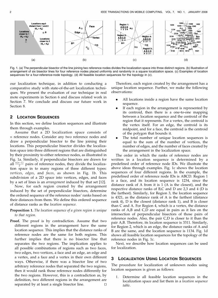
n reference nodes. Consider any two reference nodes anddraw a perpendicular bisector to the line joining theirlocations. This perpendicular bisector divides the localiza-tion space into three different regions that are distinguishedby their proximity to either reference nodes, as illustrated inFig. 1a. Similarly, if perpendicular bisectors are drawn forall nðn�1Þ

2 pairs of reference nodes, they divide the localiza-tion space in to many regions of three different types:vertices, edges, and faces, as shown in Fig. 1b. Thissubdivision of a 2D space into vertices, edges, and facesby a set of lines is an arrangement induced by that set [12].

Now, for each region created by the arrangementinduced by the set of perpendicular bisectors, determinethe ordered sequence of the reference nodes’ ranks based ontheir distances from them. We define this ordered sequenceof distance ranks as the location sequence.

Proposition 1. The location sequence of a given region is unique

to that region.

Proof. The proof is by contradiction. Assume that twodifferent regions in the arrangement have the samelocation sequence. This implies that the distance ranks ofreference nodes are the same for both regions. Thisfurther implies that there is no bisector line thatseparates the two regions. The implication applies toall possible combinations of regions such as two faces,two edges, two vertices, a face and an edge, an edge anda vertex, and a face and a vertex in their own differentways. Otherwise, if there was a bisector line of twoarbitrary reference nodes that separated the two regions,then it would rank those reference nodes differently forthe two regions. However, this is a contradiction as, bydefinition, two different regions in the arrangement areseparated by at least a single bisector line. tu

Therefore, each region created by the arrangement has aunique location sequence. Further, we make the followingobservations:

. All locations inside a region have the same locationsequence.

. If each region in the arrangement is represented byits centroid, then there is a one-to-one mappingbetween a location sequence and the centroid of theregion that it represents. For a vertex, the centroid isthe vertex itself. For an edge, the centroid is itsmidpoint, and for a face, the centroid is the centroidof the polygon that bounds it.

. The total number of unique location sequences isequal to the sum of the number of vertices, thenumber of edges, and the number of faces created bythe arrangement in the localization space.

The order in which the ranks of reference nodes arewritten in a location sequence is determined by apredefined order of reference node IDs. We illustrate theabove ideas through examples. Fig. 1c shows the locationsequences of four different regions. In the example, thepredefined order of reference node IDs is ABCD. Region 1is a face, and its location sequence is 1234, since thedistance rank of A from it is 1 (A is the closest), and therespective distance ranks of B,C and D are 2,3 and 4 (D isthe farthest). Similarly, for Region 3, the location sequenceis 4321, as the distance rank of A is the farthest (distancerank 4), D is the closest (distance rank 1), and B is closerthan C and A. For Region 4, which is a vertex, the distanceranks of A,B and C,D are equal in pairs as it lies on theintersection of perpendicular bisectors of those pairs ofreference nodes. Also, the pair C,D is closer to it than thepair A,B. Therefore, its location sequence is 3311. Similarly,for Region 2, which is an edge, the distance ranks of A andB are the same, and the location sequence is 1134. Fig. 1dshows all feasible location sequences for the topology of thereference nodes in Fig. 1c.

Next, we describe how location sequences can be usedfor localization.

3 LOCALIZATION USING LOCATION SEQUENCES

The procedure for localization of unknown nodes usinglocation sequences is given as follows:

1. Determine all feasible location sequences in thelocalization space and list them in a location sequencetable.

2 IEEE TRANSACTIONS ON MOBILE COMPUTING, VOL. 7, NO. 1, JANUARY 2008

Fig. 1. (a) The perpendicular bisector of the line joining two reference nodes divides the localization space into three distinct regions. (b) Illustration ofarrangement of six bisector lines for four reference nodes placed uniformly and randomly in a square localization space. (c) Examples of locationsequences for a four-reference-node topology. (d) All feasible location sequences for the topology in (c).

2. Determine the location sequence of the unknownnode location by using received signal strength (RSS)measurements of localization packets exchangedbetween itself and the reference nodes. The RSS-based location sequence will be a corrupted versionof the original location sequence.

3. Search in the location sequence table for the“nearest” location sequence to the unknown nodelocation sequence. The centroid mapped to by thatsequence is the location estimate of the unknownnode.

The above procedure opens itself to the followingquestions: How many feasible location sequences are therein a 2D localization space? How can we get them? How dorandom errors in RSS measurements affect the unknownnode location sequence? What is the meaning of “nearest”location sequence and how do we measure distancesbetween location sequences?

In the rest of this section, we answer the above questions.We begin by determining the maximum number of feasiblelocation sequences in the localization space.

3.1 Maximum Number of Location Sequences

For n reference nodes in the localization space, the numberof possible combination sequences of distance ranks isOðnnÞ. However, we show that the actual number of feasiblelocation sequences is much lower, which is in the order ofOðn4Þ at worst.

As stated previously, the number of feasible locationsequences is equal to the sum of the number of vertices,edges, and faces created by the arrangement induced by theperpendicular bisectors of reference nodes. Therefore, itsupper bound can be obtained by determining the maximumnumber of such vertices, edges, and faces, given thelocations of the reference nodes. In [12], the authors showthat the maximum number of vertices, edges, and faces foran arrangement induced by n lines is nðn�1Þ

2 , n2, andn2

2 þ n2 þ 1, respectively. Using these results, for nðn�1Þ

2perpendicular bisectors of n reference nodes,

1. the number of vertices is at most n4

8 � n3

4 � n2

8 þ n4 ,

2. the number of edges is at most n4

4 � n3

2 þ n2

4 , and3. the number of faces is at most n4

8 � n3

4 þ 3n2

8 � n4 þ 1.

Owing to the properties of perpendicular bisectors, it is

possible to derive tighter upper bounds on the number of

vertices, edges, and faces.

Theorem 1. Let L be the set of bisector lines for n reference nodes

jLj ¼ nðn�1Þ2 . Let AðLÞ be the arrangement induced by L.

Then,

1. the number of vertices of AðLÞ is at most n4

8 �7n3

12 þ 7n2

8 � 5n12 ,

2. the number of edges of AðLÞ is at most n4

4 � n3 þ7n2

4 � n, and3. the number of faces of AðLÞ is at most n4

8 � 5n3

12 þ7n2

8 � 7n12 þ 1.

Proof. We make use of the property that the perpendicular

bisectors of the sides of a triangle intersect at a single

point. Assume that ði� 1Þ reference nodes have already

been added, implying that the localization space already

has ði�1Þði�2Þ2 bisector lines. When the ith reference node is

added, ði� 1Þ new bisector lines are added to the

localization space.

Vertices. The first of the ði� 1Þ bisector lines intersects

the already present lines in at most ði�1Þði�2Þ2 new vertices.

The second new line is the perpendicular bisector of a

side of the triangle in which the first new line is also a

perpendicular bisector. Therefore, the second new line

has to pass through at least one of the vertices created by

the first new line, thus creating at most ði�1Þði�2Þ2 � 1 new

vertices. Similarly, the third new line creates at mostði�1Þði�2Þ

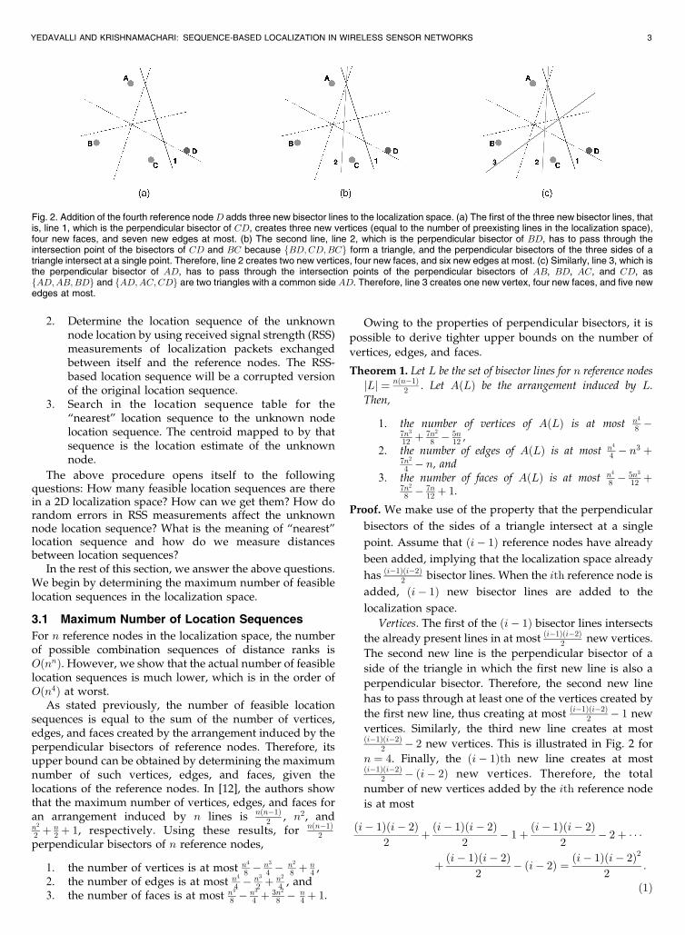
2 � 2 new vertices. This is illustrated in Fig. 2 for

n ¼ 4. Finally, the ði� 1Þth new line creates at mostði�1Þði�2Þ

2 � ði� 2Þ new vertices. Therefore, the total

number of new vertices added by the ith reference node

is at most

ði� 1Þði� 2Þ2

þ ði� 1Þði� 2Þ2

� 1þ ði� 1Þði� 2Þ2

� 2þ � � �

þ ði� 1Þði� 2Þ2

� ði� 2Þ ¼ ði� 1Þði� 2Þ2

2:

ð1Þ

YEDAVALLI AND KRISHNAMACHARI: SEQUENCE-BASED LOCALIZATION IN WIRELESS SENSOR NETWORKS 3

Fig. 2. Addition of the fourth reference node D adds three new bisector lines to the localization space. (a) The first of the three new bisector lines, thatis, line 1, which is the perpendicular bisector of CD, creates three new vertices (equal to the number of preexisting lines in the localization space),four new faces, and seven new edges at most. (b) The second line, line 2, which is the perpendicular bisector of BD, has to pass through theintersection point of the bisectors of CD and BC because fBD;CD;BCg form a triangle, and the perpendicular bisectors of the three sides of atriangle intersect at a single point. Therefore, line 2 creates two new vertices, four new faces, and six new edges at most. (c) Similarly, line 3, which isthe perpendicular bisector of AD, has to pass through the intersection points of the perpendicular bisectors of AB, BD, AC, and CD, asfAD;AB;BDg and fAD;AC;CDg are two triangles with a common side AD. Therefore, line 3 creates one new vertex, four new faces, and five newedges at most.

The maximum number of vertices for n ¼ 3 is 1.Therefore, for n reference nodes, the maximum numberof vertices is

1þXni¼4

ði� 1Þði� 2Þ2

2¼ n

4

8� 7n3

12þ 7n2

8� 5n

12: ð2Þ

Edges. As explained previously, the first new line

intersects the already present lines in at most ði�1Þði�2Þ2

vertices and creates at most ði�1Þði�2Þ2 þ 1 new edges on the

new line and at most ði�1Þði�2Þ2 new edges on the old lines,

which add up to ði�1Þði�2Þ2 � 2þ 1 new edges at most. Since

the second new line passes through at least one of

the vertices created by the first new line, it creates at

most ði�1Þði�2Þ2 þ 1 new edges on the second new line, and it

creates at most ði�1Þði�2Þ2 � 1 new edges on the old lines,

including the first new line. This adds up to at mostði�1Þði�2Þ

2 � 2 new edges in the localization space. This trend

is again illustrated in Fig. 2 for four reference nodes in the

localization space. Finally, the ði� 1Þth new line addsði�1Þði�2Þ

2 � 2� ði� 3Þ new edges to the localization space.

Therefore, the total number of new edges added by the

ith reference node is at most

ði� 1Þði� 2Þ2

� 2þ 1þði� 1Þði� 2Þ2

� 2þði� 1Þði� 2Þ2

� 2� 1

þ � � � þ ði� 1Þði� 2Þ2

� 2�ði� 3Þ ¼ i3� 9i2

2þ 15i

2� 4:

ð3Þ

The maximum number of edges for n ¼ 3 is 6.Therefore, for n reference nodes, the maximum numberof edges is

6þXni¼4

i3 � 9i2

2þ 15i

2� 4

� �¼ n

4

4� n3 þ 7n2

4� n: ð4Þ

Faces. The number of new faces created by a new line

is equal to the number of edges on the new line.

Therefore, the number of new faces created by the first

new line among the ði� 1Þ new lines is at mostði�1Þði�2Þ

2 þ 1. Since the second new line has to pass

through one of the intersection points of the first line, it

would also create ði�1Þði�2Þ2 þ 1 new faces and this trend

continues for all the ði� 1Þ new lines as illustrated in

Fig. 2. Therefore, the total number of new faces added by

the ith reference node is at most

ði� 1Þ ði� 1Þði� 2Þ2

þ 1

� �: ð5Þ

The localization space has one face when n ¼ 1.Therefore, for n reference nodes, the maximum numberof faces in the localization space is given by

1þXni¼2

ði� 1Þ ði� 1Þði� 2Þ2

þ 1

� �

¼ n4

8� 5n3

12þ 7n2

8� 7n

12þ 1: ð6Þ

tu

Corollary 1. The maximum number of unique location sequencesdue to n reference nodes is n4

2 � 2n3 þ 7n2

2 � 2nþ 1.

Proof. The maximum number of unique location sequencesis the sum of the maximum number of vertices, edges,and faces due to n reference nodes, as derived inTheorem 1:

n4

8� 7n3

12þ 7n2

8� 5n

12

� �þ n4

4� n3 þ 7n2

4� n

� �þ

n4

8� 5n3

12þ 7n2

8� 7n

12þ 1

� �¼ n4

2� 2n3þ 7n2

2� 2nþ 1:

ð7Þ

tu

Next, we illustrate how we can obtain all these feasiblelocation sequences in the localization space and store themin the location sequence table.

3.2 Location Sequence Table Construction

Below, we present the pseudocode for an algorithm thatconstructs the location sequence table, given the locations ofthe reference nodes and the boundaries of the localizationspace:1

Algorithm 1: CONSTRUCTLOCATIONSEQUENCETABLE.

Input:

1) Location coordinates of reference nodes

fðaxi; ayiÞji ¼ 0! n� 1g.2) Boundaries of the localization space B.

Output: Location Sequence Table.

0 L ¼ fliji ¼ 0! ðnðn�1Þ2 � 1Þg

BISECTORLINES(fðaxi; ayiÞji ¼ 0! n� 1g; B)

1 ðFL;EL; V LÞ CONSTRUCTARRANGEMENTðLÞ.Get vertex sequences.

2 for i 0 to ðjV Lj � 1Þ3 Centroid½i� V L½i�4 Sequence½i� GETSEQUENCEðCentroid½i�Þ5 end for

.Get edge sequences.

6 for i jV Lj to ðjV Lj þ jELj � 1Þ7 Centroid½i� GETEDGECENTROIDðEL½i�Þ8 Sequence½i� GETSEQUENCEðCentroid½i�Þ9 end for

.Get face sequences.

10 for i ðjV Lj þ jELjÞ to ðjV Lj þ jELj þ jFLj � 1Þ11 Centroid½i� GETFACECENTROIDðFL½i�Þ12 Sequence½i� GETSEQUENCEðCentroid½i�Þ13 end for

.Return the location sequence table

14 return {Sequence, Centroid}

. BISECTORLINES takes in the locations of the refer-ence nodes and the boundaries of the localizationspace as input and returns the set L of all pairwiseperpendicular bisector lines within the boundaries ofthe localization space. Each line is represented by the

4 IEEE TRANSACTIONS ON MOBILE COMPUTING, VOL. 7, NO. 1, JANUARY 2008

1. C++ code files that construct the arrangement of lines and thelocation sequence table are available for download at http://anrg.usc.edu/downloads.html.

intersection points on the left and right boundariesof the localization space.

. CONSTRUCTARRANGEMENT constructs the arrange-ment, given a set of lines as input, and returns adoubly connected edge list (EL) that consists of avertex list ðV LÞ, an EL, and a face list ðFLÞ. Pleaserefer to [12] (Section 8.3) for a detailed description ofthis algorithm.

. VL contains pointers to all vertices of the arrange-ment induced by the set L.

. EL contains pointers to all edges of the arrangementinduced by the set L.

. FL contains pointers to all faces of the arrangementinduced by the set L.

. GETEDGECENTROID takes in an edge pointer as theinput and returns the centroid of the edge. Thecentroid of an edge ðcx; cyÞ is its midpoint, given by

ðcx; cyÞ ox þ dx

2;oy þ dy

2

� �; ð8Þ

where ðox; oyÞ and ðdx; dyÞ are the origin and

destination vertices of the edge.. GETFACECENTROID takes in a face pointer as

the input and returns the centroid of the face.The centroid of a face ðcx; cyÞ, given its verticesfðxi; yiÞj0 � i � p� 1g, is calculated as follows:

cx 1

6A

Xp�1

i¼0

ðxi þ xiþ1Þðxiyiþ1 � xiþ1yiÞ; ð9Þ

cy 1

6A

Xp�1

i¼0

ðyi þ yiþ1Þðxiyiþ1 � xiþ1yiÞ; ð10Þ

where p is the number of vertices that bound a given

face and A is its area given by

A 1

2

Xp�1

i¼0

ðxiyiþ1 � xiþ1yiÞ ; ðxp; ypÞ ¼ ðx0; y0Þ: ð11Þ

. GETSEQUENCE takes in the coordinates of a point inthe localization space and returns the locationsequence for that point with respect to the locationsof the reference nodes.

Theorem 2. Algorithm 1 takes Oðn5 logðnÞÞ worst case time and

Oðn5Þ worst case space to construct the location sequence

table.

Proof. The function BISECTORLINES in line 0 takes Oðn2Þtime and space. The algorithm CONSTRUCTARRANGE-

MENT that constructs the arrangement of linestakes Oðn4Þ time, which is optimal, as proven in [12,Theorems 8.5 and 8.6]. Since this algorithm returns theVL, the EL, and the FL, it requires Oðn4Þ space to storeall the three lists. The functions GETFACECENTROID

and GETEDGECENTROID in lines 3 and 7, respectively,take Oð1Þ time and space each. The function GET-

SEQUENCE involves sorting n reference nodes basedon their distances from the centroid of the region in

consideration. This takes Oðn lognÞ time and OðnÞspace. Since the number of faces, edges, and verticesis Oðn4Þ, the worst case time requirement for lines 2-13in the above algorithm is Oðn5 log ðnÞÞ and the worstcase space requirement is Oðn5Þ. Therefore, in total,Algorithm 1 takes Oðn5 logðnÞÞ worst case time andOðn5Þ worst case space to construct the locationsequence table. tuNext, we discuss the effect of RF channel random errors

on the unknown node location sequence.

3.3 Unknown Node Location Sequence

The unknown node determines its location sequence byusing RSS measurements of RF localization packets ex-changed between itself and the reference nodes. The RSSmeasurements are subjected to random errors due to RFchannel nonidealities such as multipath and shadowing. Inthe absence of such nonidealities, the RSS measurementsaccurately represent the distances between the unknownnode and the reference nodes. If the reference nodes areranked in a decreasing order of these RSS values, then thisorder represents the increasing order of their separationfrom the unknown node.

This is not true in reality. Reference nodes that arefarther from the unknown node might measure higher RSSvalues than reference nodes that are closer. If the referencenodes are ranked on their respective RSS measurements,then the location sequence formed by these ranks will be acorrupted version of the original sequence. Corruption in anunknown node location sequence results in an erroneousestimation of its location. In the ideal case, when there is nocorruption, the unknown node location would be thecentroid of the region represented by its location sequence.However, corruption in its location sequence could erro-neously estimate its location to be the centroid of someother region.

For example, if the ranks of reference nodes C and D areinterchanged because of corruption due to RF channelnonidealities for Region 1 in Fig. 1c, then the new locationsequence would be 1243 instead of 1234. Moreover, 1243represents a region that is adjacent to the original region, asshown in Fig. 1d.

3.4 Feasible and Infeasible Sequences

As discussed previously, combinatorially, n reference nodesproduce OðnnÞ location sequences. However, as shown inthe previous section, a localization space with n referencenodes has only Oðn4Þ distinct regions and, consequently,

YEDAVALLI AND KRISHNAMACHARI: SEQUENCE-BASED LOCALIZATION IN WIRELESS SENSOR NETWORKS 5

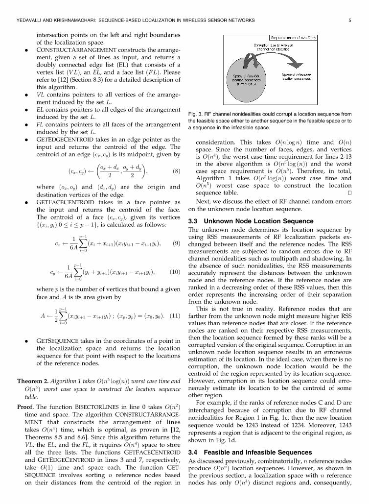
Fig. 3. RF channel nonidealities could corrupt a location sequence from

the feasible space either to another sequence in the feasible space or to

a sequence in the infeasible space.

only Oðn4Þ feasible location sequences in the worst case. Forgiven reference node locations, the location sequence tableincludes all feasible location sequences. All other sequencesare infeasible. The nonidealities of the RF channel couldcorrupt a feasible location sequence either to anotherfeasible sequence or to an infeasible sequence, as illustratedin Fig. 3. If the corrupted sequence is infeasible, then itwould be possible to detect the corruption in the sequence,whereas, if the corrupted sequence is feasible, thencorruption detection is not possible.

Here, we would like to emphasize the importance of lowdensity of location sequences compared to the full sequencespace. The low density of location sequences implies thatmany infeasible sequences are mapped to a single feasiblesequence, and this, in turn, could provide robustness tolocation estimation against RF channel nonidealities.

Next, we present metrics to measure the distancebetween two location sequences.

3.5 Distance Metrics

The distance between two location sequences is essentiallythe difference in rank orders of different reference nodes.Fortunately, statistics [13] offers two metrics that capturethis difference in rank orders: Spearman’s Rank OrderCorrelation Coefficient and Kendall’s Tau.

Given two location sequences U ¼ fuig and V ¼ fvig,1 � i � n, where ui and vi are the ranks of reference nodes,the above two metrics are defined as follows:

1. Spearman’s Rank Order Correlation Coefficient [13]. It isdefined as the linear correlation coefficient of theranks and is given by

� ¼ 1� 6Pn

i¼1ðui � viÞ2

nðn2 � 1Þ : ð12Þ

2. Kendall’s Tau [13]. In contrast to Spearman’s coeffi-cient, in which the correlation of exact ranks iscalculated, this metric calculates the correlationbetween the relative ordering of ranks of the twosequences. It compares all the nðn�1Þ

2 possible pairs ofranks ðui; viÞ and ðuj; vjÞ to determine the number ofmatching and nonmatching pairs. A pair is matchingor concordant if ui > uj ) vi > vj or ui < uj ) vi <vj and nonmatching or discordant if ui > uj ) vi <vj or ui < uj ) vi > vj. The correlation between thetwo sequences is calculated as follows:

� ¼ ðnc � ndÞffiffiffiffiffiffiffiffiffiffiffiffiffiffiffiffiffiffiffiffiffiffiffiffiffiffiffiffinc þ nd þ ntup ffiffiffiffiffiffiffiffiffiffiffiffiffiffiffiffiffiffiffiffiffiffiffiffiffiffiffi

nc þ nd þ ntvp ; ð13Þ

where nc is the number of concordant pairs, nd is thenumber of discordant pairs, ntu is the number of tiesin u, and ntv is the number of ties in v.

The range of both � and � is [�1, 1]. Next, we describe theprocedure to determine the locations of unknown nodes byusing their location sequences.

3.6 Location Determination

The location of the unknown node is determined as follows:

1. Calculate distances between the unknown nodelocation sequence and all location sequences in the

location sequence table by using the above distancemetrics.

2. Choose the centroid represented by the locationsequence that is closest to the unknown nodelocation sequence as its location estimate.

Mathematically,

LocationEstimate ¼ Centroidðarg min1�i�Oðn4Þ

�iÞ; ð14Þ

where �i is the Kendall’s Tau or Spearman’s correlationbetween the unknown node location sequence and theith location sequence in the location sequence table.

Due to RF channel nonidealities, the unknown nodelocation sequence could be a feasible sequence differentfrom its uncorrupted version or an infeasible sequence. Inany case, the above procedure maps it to the centroid of thenearest feasible location sequence in the location sequencetable that represents a different region in the arrangementthan the original uncorrupted version.

We measure the amount of corruption in the unknownnode location sequence by calculating its distance from theuncorrupted version, using the above metrics, and denote itby T . We denote the distance between the corruptedunknown node location sequence and the nearest feasiblesequence in the location sequence table by � .

Calculating the Spearman’s coefficient and Kendall’s Taubetween two sequences are OðnÞ and Oðn2Þ operations,respectively. Since the location sequence table is of sizeOðn4Þ, searching through it takes Oðn5Þ and Oðn6Þ opera-tions, respectively, for the above two metrics. Later in thepaper, in Section 5, we compare the performance of the twodistance metrics in terms of error in the unknown nodelocation estimate.

4 LOCALIZATION SCENARIOS

In this section, we illustrate two localization procedures fortwo different scenarios that are determined by the localiza-tion space size:

1. The entire localization space is within the radio range ofthe unknown node. In this case, the location sequencetable remains constant for all locations of theunknown node in the localization space. Therefore,the localization procedure is given as follows:

. Preconstruct and store the location sequencetable by using the locations of the referencenodes.

. When the unknown node initiates the localiza-tion process by broadcasting a localizationpacket, provide the stored location sequencetable along with the RSS measurements fromthe reference nodes.

. The unknown node determines its locationsequence by using the RSS measurements anddetermines its location by searching through theprovided location sequence table for the nearestfeasible location sequence.

Here, the time cost incurred by the unknown node toestimate its location is equal to the sum of the time todetermine its location sequence, which is anOðn lognÞ operation, and the time to search through

6 IEEE TRANSACTIONS ON MOBILE COMPUTING, VOL. 7, NO. 1, JANUARY 2008

the location sequence table, which is a Oðn6Þoperation. The amount of memory space requiredis on the order of Oðn5Þ bytes.

2. The localization space is much larger than the radio rangeof the unknown node. In this case, the locationsequence table changes with the location of theunknown node as a different set of reference nodesare encountered at each location. Therefore, thelocalization procedure is given as follows:

. The unknown node collects the locations andRSS measurements of the reference nodes in itsradio range.

. It constructs the location sequence table byusing Algorithm 1 and the locations of thereference nodes and calculates its locationsequence by using the RSS measurements.

. It determines its location by searching for thenearest sequence in the location sequence table.

In this case, the time cost incurred by the unknownnode to estimate its location is equal to the sum ofthe time to calculate its location sequence, which isan Oðn lognÞ operation, the time to construct thelocation sequence table, which is an Oðn5 lognÞoperation, and the time to search through it, whichis a Oðn6Þ operation. The memory requirement isOðn5Þ in this case also.

A wireless device that is typically used as an unknownnode is of the form factor of an iPAQ [14] (that cancommunicate with the reference node devices, usually ofthe form factor of Berkeley MICA 2 motes [15]) whichtypically has a 300-MHz processor and 128-Mbyte RAM. Inreal-application scenarios, a typical value for the number ofreference nodes ðnÞ is less than 15, after which there is onlya very marginal gain in location accuracy of the unknownnode. Therefore, for a typical value of n ¼ 10 referencenodes, the time and space requirements for the unknownnode to construct the location sequence table are approxi-mately 0.3 ms and 32 Kbytes, respectively. Also, the timerequired to search through it is approximately 0.45 ms.Thus, including the associated overhead, the total localiza-tion time taken by SBL is in milliseconds in typicalapplication scenarios, which is very efficient. Next, we

illustrate the robustness of our localization technique toRF channel nonidealities through some examples.

4.1 Examples

Fig. 4 shows a sample layout of nine reference nodes placedin a grid and a single unknown node (P). Fig. 4a plots thelocation estimate (E) for the ideal case when there are noerroneous ranks; that is, the location sequence is uncor-rupted, or T ¼ 1. In these examples, we use Kendall’s Tauto measure the distance between sequences. Figs. 4b, 4c, and4d show the location estimates for increasing corruption inunknown node location sequences. The location estimateerror increases with increasing corruption or decreasingcorrelation T between the RSS location sequence and thetrue location sequence of P. These examples suggest thatSBL is robust to multipath and shadowing effects of the RFchannel up to some level. Intuitively, the three main reasonsto which this robustness can be attributed to are

1. the low density Oðn4Þ of the location sequencespace relative to the entire sequence space of OðnnÞ,

2. the inherent redundancy of comparing nðn�1Þ2 rank

pairs in calculating the distance between twosequences by using Kendall’s Tau, and

3. the rank order in the location sequence of theunknown node due to two reference nodes withpath losses PLi and PLj, which is robust to randomerrors in them up to a tolerance level of jPLi � PLjj.

5 EVALUATION

In this section, we present a complete performanceevaluation of SBL. First, we discuss its inherent locationerror characteristics, and then, by using simulations, westudy its performance as a function of the RF channel andnode deployment parameters. We also present a compara-tive study with three other state-of-the-art localizationtechniques.

5.1 Location Error Characteristics

In the location sequence table, each location sequence mapsto the centroid of the region that it represents. Representingall locations in a region by its centroid comes at the cost of

YEDAVALLI AND KRISHNAMACHARI: SEQUENCE-BASED LOCALIZATION IN WIRELESS SENSOR NETWORKS 7

Fig. 4. Robustness examples: location estimate (E) for the unknown node (P) at (1,3) for a grid layout of nine reference nodes. The number adjacentto a reference node is its corresponding rank. The location error is expressed in meters, where the side length of the square localization area is 12 m.(a) ðT ¼ 1; � ¼ 1Þ, Estimate (E): (1.33, 1.33), and Location Error: 0.46 m. (b) ðT ¼ 0:722; � ¼ 0:783Þ, Estimate (E): (2.0, 2.0), and Location Error:1.4 m. (c) ðT ¼ 0:556; � ¼ 0:667Þ, Estimate (E): (2.0, 2.0), and Location Error: 1.4 m. (d) ðT ¼ 0:111; � ¼ 0:278Þ, Estimate (E): (2.0, 1.33), andLocation Error: 1.94 m.

error in the location estimate of the location sequence. Forface regions (in which the unknown node is more likely tobe located), the location error is of the order of the squareroot of the area of the face. Since the number of faces forn reference nodes is Oðn4Þ, the average face area varies,which is proportional to 1

n4 . Therefore, the average locationestimate error for locations in a face region reduces, whichis proportional to n2.

Apart from the above location errors, the performance ofSBL is affected by random errors in RSS measurements dueto multipath and shadowing effects of the RF channel. Inthe rest of this section, we present results from simulationstudies that capture the effect of these random errors on theperformance of SBL.

5.2 Simulation Model

The most widely used simulation model to generate RSSsamples as a function of distance in RF channels is the log-normal shadowing model [16]:

PRðdÞ ¼ PT � PLðd0Þ � 10� log10

d

d0 þX�; ð15Þ

where PR is the received signal power, PT is the transmitpower, and PLðd0Þ is the path loss for a reference distanceof d0. � is the path loss exponent, and the random variationin RSS is expressed as a Gaussian random variable of zeromean and �2 variance X� ¼ Nð0; �2Þ. All powers are indBm, and all distances are in meters. In this model, we donot provision separately for any obstructions like walls. Ifobstructions are to be considered, then an extra constantneeds to be subtracted from the right-hand side of the aboveequation to account for the attenuation in them (theconstant depends on the type and number of obstructions).

5.3 Simulation Parameters

The accuracy of RF-based localization techniques dependson a number of parameters. Chief among these is theaccuracy of RSS measurements. In an ideal world, in whichRSS values are not affected by multipath fading effects, theyrepresent true distances between nodes, which can lead tovery accurate localization of unknown nodes. The idealworld is represented by � ¼ 0 in (15). However, in the realworld, RSS values are corrupted by multipath fadingeffects. This has a profound influence on the accuracy ofRF localization techniques. According to the above propa-gation model, RSS values are defined by � and � values forthe given environment. Since every RF environment can becharacterized by � and � values (see [17] and [18]), it isnecessary to study the accuracy of RF localization techni-ques as a function of these two parameters.

In addition, the density and number of reference nodesavailable to the unknown node has a significant influenceon the number of reference nodes (see [2], [6], and so forth).Thus, the location estimate of any RF-based localizationtechnique depends on a fundamental set of parameters,which can be broadly categorized as follows:

1. RF Channel Characteristics [17], [16]:

. Path loss exponent ð�Þ: measures the powerattenuation of RF signals relative to distance.

. Standard deviation ð�Þ: measures the standarddeviation in RSS measurements due to log-normal shadowing.

The values of � and � change with the frequency ofoperation and the obstructions and disturbance inthe environment.

2. Node Deployment Parameters:

. Number of reference nodes ðnÞ and

. Reference node density ð�Þ.Table 1 lists the typical values and ranges for different

parameters used in our simulations.

5.4 Simulation Procedure

We assume that all reference nodes are in the radio range ofeach other and also that of the unknown node. A 48-bitarithmetic linear congruential pseudorandom number gen-erator was used, and results were averaged over 100 ran-dom trials. In each trial, n reference nodes were placeduniformly and randomly in a square localization space ofsize S � S square meters, and the unknown node wasplaced at 100 different locations on a grid of S

10 separation.In total, the results presented are averaged over 10,000different scenarios. In our simulations, we use S ¼ 100 m.

The performance of SBL is measured in terms of locationerror for a wide range of RF channel conditions and nodedeployment parameters. Location error is defined as theeuclidean distance between the location estimate and theactual location of the unknown node. The location error isaveraged over 100 random trials, as described previously.

Fig. 5 plots the two distance metrics described in theprevious section as a function of the number of referencenodes ðnÞ or, in other words, the length of the locationsequence. There is a growing difference, however small,between the two metrics with increasing length of the

8 IEEE TRANSACTIONS ON MOBILE COMPUTING, VOL. 7, NO. 1, JANUARY 2008

TABLE 1Typical Values and Ranges for Different Simulation Parameters

Fig. 5. Average location error as measured using Spearman’scorrelation and Kendall’s Tau as a function of the number of referencenodes.

sequence, with Kendall’s Tau performing increasingly

better than Spearman’s correlation in terms of the locationestimate error.

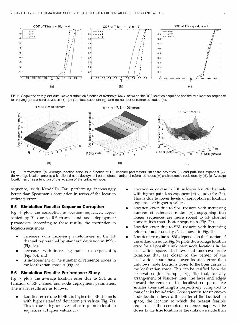
5.5 Simulation Results: Sequence Corruption

Fig. 6 plots the corruption in location sequences, repre-

sented by T , due to RF channel and node deployment

parameters. According to these results, the corruption in

location sequences

. increases with increasing randomness in the RFchannel represented by standard deviation in RSS �(Fig. 6a),

. decreases with increasing path loss exponent �(Fig. 6b), and

. is independent of the number of reference nodes inthe localization space n (Fig. 6c).

5.6 Simulation Results: Performance Study

Fig. 7 plots the average location error due to SBL as a

function of RF channel and node deployment parameters.The main results are as follows:

. Location error due to SBL is higher for RF channelswith higher standard deviation ð�Þ values (Fig. 7a).This is due to higher levels of corruption in locationsequences at higher values of �.

. Location error due to SBL is lower for RF channelswith higher path loss exponent ð�Þ values (Fig. 7b).This is due to lower levels of corruption in locationsequences at higher � values.

. Location error due to SBL reduces with increasingnumber of reference nodes ðnÞ, suggesting thatlonger sequences are more robust to RF channelnonidealities than shorter sequences (Fig. 7b).

. Location error due to SBL reduces with increasingreference node density �, as shown in Fig. 7b.

. Location error due to SBL depends on the location ofthe unknown node. Fig. 7c plots the average locationerror for all possible unknown node locations in thelocalization space. It shows that unknown nodelocations that are closer to the center of thelocalization space have lower location error thanunknown node locations closer to the boundaries ofthe localization space. This can be verified from theobservation (for example, Fig. 1b) that, for anyarrangement of bisector lines, the faces and edgestoward the center of the localization space havesmaller areas and lengths, respectively, compared tothat of at its boundaries. Consequently, for unknownnode locations toward the center of the localizationspace, the location to which the nearest feasiblesequence of the corrupted sequence maps will becloser to the true location of the unknown node than

YEDAVALLI AND KRISHNAMACHARI: SEQUENCE-BASED LOCALIZATION IN WIRELESS SENSOR NETWORKS 9

Fig. 6. Sequence corruption: cumulative distribution function of Kendall’s Tau T between the RSS location sequence and the true location sequencefor varying (a) standard deviation ð�Þ, (b) path loss exponent ð�Þ, and (c) number of reference nodes ðnÞ.

Fig. 7. Performance. (a) Average location error as a function of RF channel parameters: standard deviation ð�Þ and path loss exponent ð�Þ.(b) Average location error as a function of node deployment parameters: number of reference nodes ðnÞ and reference node density ð�Þ. (c) Averagelocation error as a function of the location of the unknown node.

for locations toward the boundaries. This results inlower location errors for unknown node locationstoward the center of the localization space than forlocations toward its boundaries.

. Fig. 8a plots the average location error as a functionof Kendall’s Tau values T and � , and Fig. 8b plots �as a function of T . The figures suggest the following:

– The location error is correlated to T , which is thecorruption due to RF channel.

– The location error is correlated to � , which is thedistance between the corrupted sequence andthe nearest feasible sequence.

– A correlation exists between � and T .

This suggests that � , which is a measurable quantity,

as opposed to T , could be used as a quantitative

indicator of the location error due to SBL. Also,

owing to its correlation to T , it could also be used as

an approximate indicator of the state of the RF

channel.

5.7 Simulation Results: Comparative Study

We compare SBL with three other comparable (see [19])

state-of-the-art localization techniques: least squares estimator

(LSE), proximity localization, and three centroid.

. LSE. It is identical to the maximum likelihoodlocation estimator [1], [2] and works as follows:

– Measure the distance between each of thereference nodes and the unknown node byusing

dmi ¼ 10PT�PLðd0Þ�PRi

10� ; ð16Þ

where dmi is the measured distance and PRi is

the mean received signal power between a given

reference node i and the unknown node.

Accurate distance measurement requires accu-

rate estimation of the path loss exponent ð�Þ of

the environment. This requires expensive ran-

ging techniques and/or extensive preconfigura-

tion surveys of the localization space.– For each grid point location in the localization

space, determine the sum of the squares ofdifferences in the measured distances and the

true euclidean distances of all the referencenodes from the grid point:

�ðx;yÞ ¼Xn�1

i¼0

ðdðx;yÞi � dmiÞ2; ð17Þ

where dðx;yÞi is the euclidean distance between

the grid location ðx; yÞ and the reference node i.– Choose the grid point location with the least

value of the above sum �ðx;yÞ as the location of

the unknown node. In our study, we consider a

grid resolution ðrÞ that is 100 times higher than

the dimensions of the localization space; that is,for a localization space of S � S square meters,

we search r2 ¼ 10; 000 grid points, with a

separation of S100 meters between them, to

determine the location of the unknown node.. Proximity localization. The location of the closest

reference node by RSS value is chosen as the locationof the unknown node. This is an extreme special caseof SBL, in which the sequence is of length 1.

. Three centroid. The centroid of all the reference nodesin the radio range of the unknown node is chosen asits location [7]. Since, in our case, all reference nodesare in the radio range of the unknown node, thelocation error would be independent of the RFchannel characteristics. In order to measure theeffect of these characteristics on the centroid techni-que, we choose the centroid of the closest threereference nodes by RSS values as the location of theunknown node.

Fig. 9 plots the average location error due to SBL, LSE,proximity localization, and three centroid as a function ofthe standard deviation in RSS log-normal distribution � fordifferent values of path loss exponents � and for differentvalues of number of reference nodes n. The main results ofthe comparison are the following:

. SBL performs better than proximity localization andthree centroid over a range of RF channel and nodedeployment parameters.

. SBL performs better than LSE for higher values of �,whereas LSE performs better than SBL for lowervalues of �. There is a crossover value of � betweenthe error due to SBL and LSE, and this value of � ishigher for environments that have more attenuation,that is, higher values of path loss exponent �. Thereis no significant change in the value of crossover �with changing number of reference nodes n.

. For lower values of �, the location error due to SBLdecreases faster than location error due to LSE forincreasing values of n. This can be seen in Figs. 9a,9b, and 9c, in which the difference between thelocation error due to SBL and LSE reduces withincreasing values of n.

. LSE is outperformed by all other localizationtechniques after some value of �, and this value isthe lowest for SBL.

It should be noted that, in the above simulations, LSEoperates at a considerable advantage over other techniquesas the exact value of the path loss exponent � is known. This

10 IEEE TRANSACTIONS ON MOBILE COMPUTING, VOL. 7, NO. 1, JANUARY 2008

Fig. 8. (a) Average location error as a function of the sequencecorruption ðT Þ and as a function of the distance ð�Þ between thecorrupted sequence and its nearest feasible sequence in the locationsequence table. (b) Correlation between � and T .

advantage vanishes in real-world scenarios, where thevalue of � is very difficult to estimate accurately, owing toits dependence on the area features such as walls, furniture,and so forth. Thus, LSE may not perform as well in real-world scenarios. Table 2 compares the time and spacecomplexities of SBL with that of the other three localizationtechniques. We believe that the efficiency of SBL can beincreased significantly by using more efficient locationsequence table search algorithms as opposed to a naivesearch.

6 REAL-WORLD EXPERIMENTS

The performance of SBL in real systems is studied through

two experiments, representing different RF channel and

node deployment parameters, and conducted using Berke-

ley MICA 2 motes [15]. The first experiment was conducted

in a parking lot, which represents a relatively obstruction-

free RF channel, and the second experiment was conducted

in an office building with many rooms and furniture, which

represents a typical indoor environment. For comparison,

the locations of the unknown nodes were also estimated

using the three localization techniques—LSE, proximity

localization, and three centroid—described in the previous

section.

6.1 Outdoor Experiment: Parking Lot

The RF channel in an outdoor parking lot represents a classof relatively obstruction-free channels. As shown in Fig. 10,11 MICA 2 motes were placed randomly on the ground. Allmotes were in the line of sight of each other, and all of themwere programmed to broadcast a single packet withoutinterfering with each other.2 The motes recorded the RSSvalues of the received packets and stored them in theirelectrically erasable programmable read-only memory(Eeprom), which were later used offline for locationestimation.

The locations of all the motes were estimated andcompared with their true locations. Since all motes werein the radio range of each other, each mote had 10 referencenodes. For the LSE method, to estimate the distancesbetween the motes, the RSS model described by (15) inSection 5.2 was used, as there were no obstructions betweenthe motes in this experiment. The performance of the LSEtechnique depends on the value of the path loss exponent �for the area in which the experiment was conducted. Forthis experiment, we used the true distances and thecorresponding RSS values between the reference nodesand the unknown node to estimate the value of �. Fig. 10aplots the RSS values as a function of distance. Linearregression analysis applied to the RSS versus distance datagives its slope as �2.9, implying that � ¼ 2:9. We used thisvalue of � to evaluate the LSE technique.

Fig. 10b compares the true mote locations with SBLlocation estimates for all the motes. The figure also showsthe arrangement induced by the perpendicular bisectors

YEDAVALLI AND KRISHNAMACHARI: SEQUENCE-BASED LOCALIZATION IN WIRELESS SENSOR NETWORKS 11

2. We had actually measured the RSS of 100 packets in 1 minute andobserved that their standard deviation was less than 0.5 dBm. Therefore, wedecided to use only a single packet for localization. In real-applicationscenarios, this would help in conserving energy at the mote and reducingthe delay in localization without affecting its accuracy.

Fig. 9. Comparison: average location error due to SBL, LSE, proximity localization, and three centroid as a function of the standard deviation of RSS

log-normal distribution � for different values of path loss exponent � ((a) � ¼ 2, and n ¼ 10, (b) � ¼ 4, and n ¼ 10, and (c) � ¼ 6, and n ¼ 10) and for

different values of number of reference nodes n ((a) n ¼ 4, and � ¼ 4, (b) n ¼ 7, and � ¼ 4, and (c) n ¼ 10, and � ¼ 4).

TABLE 2Comparison of Worst Case Computational Complexitiesof SBL, LSE, Proximity Localization, and Three Centroid

between all pairs of reference nodes. Fig. 10c plots theabsolute error in meters at each mote location due to all thefour techniques. Evidently, SBL performs better thanproximity localization and three centroid in 10 out of11 cases, and it performs better than LSE in all the 11 cases.

Fig. 10d plots the sequence corruption ðT Þ at each motelocation and the distance ð�Þ between the corruptedsequence and the nearest feasible sequence in the locationsequence table for all the 11 nodes. The correlation betweenT and � can be clearly seen in the figure. Comparing Fig. 10cand Fig. 10d, broad correlations between T and the locationerror and between � and the location error can be observedfor SBL. For example, the location error is the highest fornode IDs 1 and 9, in that order, and � is the lowest for thesame node IDs in the same order. Also, the location error isalmost equal for nodes 8, 2, 7 and 10. This trend is alsoreflected in the values of � for those nodes.

Table 3 shows the average absolute location error inmeters, with varying numbers of reference nodes consid-ered by the unknown node. For each node in theexperiment, n reference nodes were chosen in turn fromthe 10 available reference nodes. Thus, for n referencenodes, the location error is averaged over 10

n

� �values. The

table shows that, in an outdoor environment, SBL performsbetter than the other three localization techniques, irrespec-tive of the number of reference nodes.

6.2 Indoor Experiment: Office Building

Office buildings with features such as rooms, corridors,furniture, and other obstructions represent a distinct classof RF channels. We placed 12 MICA 2 motes (referencenodes) on the ground randomly in a corner of the ElectricalEngineering building at the University of Southern Cali-fornia (USC), spanning different rooms and corridors.Fig. 11 shows a schematic of the experimental setup. Inthis experiment, an unknown node was placed at five

different locations, and these locations were estimatedusing all the 12 motes as reference nodes. As in the outdoorexperiment, the unknown node was programmed tobroadcast a single packet from each location, and thereference nodes recorded the RSS values of this packet intheir respective Eeprom, which were later used offline forlocation estimation.

Unlike in the outdoor experiment, not all motes were inthe line of sight of each other, even though they were ineach other’s radio range. A subset of the motes hadobstructions in between them in the form of walls. As forthe outdoor experiment, for the LSE method, the value of �was calculated using linear regression analysis for RSSversus distance values between the reference nodes and theunknown node. Fig. 11a shows the data. In this case, thevalue of � is 2.2.

Fig. 11b compares the SBL location estimates of the fiveunknown node locations with their true locations. It can beseen that the path of the location estimates closely followsthe true path of the unknown node. Fig. 11c plots thelocation estimate error due to SBL, LSE, proximity localiza-tion, and three-centroid techniques for each unknown nodelocation. It can be observed that SBL performs better thanLSE and three centroid in four out of five cases and betterthan proximity localization in two out of five cases. Thereason that proximity localization is performing well is thepresence of reference nodes in close proximity to eachlocation of the unknown node.

Fig. 11d plots the sequence corruption ðT Þ at each motelocation and the distance ð�Þ between the corruptedsequence and the nearest feasible sequence in the locationsequence table for all the five unknown node locations.Comparing this figure and Fig. 10d shows that sequencesare more corrupted in the indoor experiment than theoutdoor experiment, which was expected. Also, as in theoutdoor experiment, there is a clear correlation between Tand � for the indoor experiment. However, the correlationsbetween T and location error and between � and locationerror are not as clear as that in the outdoor experiment.

Table 4 shows the average absolute location error inmeters, with varying numbers of reference nodes consid-ered by the unknown node. Similar to the outdoorexperiment, for each node in the experiment, n referencenodes were chosen in turn from the 12 available referencenodes and, thus, for n reference nodes, the location error isaveraged over 12

n

� �values. The table shows that, in this

12 IEEE TRANSACTIONS ON MOBILE COMPUTING, VOL. 7, NO. 1, JANUARY 2008

Fig. 10. Outdoor experiment: 11 MICA 2 motes placed randomly in an area of 144 square meters were used as reference nodes and unknown

nodes. Consequently, each unknown node had 10 reference nodes. (a) Path loss exponent calculation � ¼ 2:9. (b) Comparison between true

locations and SBL location estimates. (c) Location error due to SBL, LSE, proximity localization, and three centroid (the nodes are ordered in

increasing error of SBL). (d) Corruption measure T and error indicator � .

TABLE 3Comparison of Average Location Errorin Meters for the Outdoor Experiment

scenario, SBL outperforms LSE for all the cases and thatproximity localization (which is an extreme special case ofSBL) performs better than SBL. As mentioned previously,the reason for this is that the choice of unknown nodelocations is such that there is a reference node in closeproximity to each such location.

6.3 Discussion

Experimental results show that localization techniques aremore accurate for relatively clutter-free RF channel envir-onments (outdoors with line of sight) than RF channels withmany obstructions (indoor environment). Also, the perfor-mance of LSE in real-world scenarios is worse than insimulations, as conjectured in Section 5.7. This is mainlybecause the radio propagation model of (15) is anapproximate model, and the location estimate accuracy forthe LSE technique depends heavily on the accuracy of the� estimate. The RSS measurements in the experimentsdepend on antenna orientations, antenna height, andtransmitter/receiver nondeterminism. For simulations,these issues can be captured within the log-normal randomterm in (15).

7 RELATED WORK

In an earlier work [19], we presented a novel localizationalgorithm called Ecolocation that uses location constraints forrobust localization. A location constraint is a relationshipbetween the distances of two reference nodes from theunknown node that determines its proximity to eitherreference nodes, as shown in Fig. 1a. Location constraintscan be graphically represented by perpendicular bisectorsbetween reference nodes (Section 2), and each locationsequence can be written as a set of location constraints.Thus, the location constraint set is also unique to eachregion in the arrangement.

In this localization algorithm, the unknown nodedetermines its set of location constraints by using RSSmeasurements and estimates its location by searchingthrough grid points in the localization space to determinethe grid point with the highest number of matched locationconstraints. In [19], we show that this is an Oðn2S2

r2 Þ timeoperation, where S is the side of the square localizationspace and r is the resolution of grid points. Thus, thelocalization algorithm using location constraints is depen-dent on the localization space size, the resolution of thegrid points, and the number of reference nodes. In contrast,the localization algorithm using location sequences de-pends only on the number of reference nodes, albeitat higher time cost of Oðn6Þ. In fact, constraint-basedlocalization results tend to SBL ones for very high values ofgrid point resolution r. The cost differences suggest that,for smaller localization spaces and lower location accuracyrequirements, a constraint-based localization is bettercompared to a sequence-based one, whereas the reverseis true for bigger localization spaces and higher locationaccuracy requirements.

In related works, Chakrabarty et al. [9] and Ray et al. [10]use identity codes to determine the location of sensor nodesin grid and nongrid sensor fields, respectively. Here, eachgrid point or region in the localization space is identified bya unique set of reference node IDs whose signals can reachthe point or region, and this unique set is an identity codefor that point or region. The two main drawbacks of thisapproach are that 1) in order to uniquely identify allunknown node locations in the localization space, thereference nodes need to be placed carefully according torules determined by an optimization algorithm, andthat 2) for acceptable location accuracies, the number ofreference nodes required is prohibitively expensive, and forsparse networks of reference nodes, the accuracy is coarsegrained in the order of radio range. For example, thenumber of reference nodes required to uniquely identify thelocation of an unknown node using identity codes is OðpmÞ,where m is the number of dimensions of the localizationspace, and p is the number of grid points per dimension [9].

In another related work, He et al. [6] propose an RF-based localization technique in which the unknown nodelocation is determined by the intersection of all triangles,formed by reference nodes, that are likely to bound it. Theunknown node determines its existence inside a triangle bycomparing its measured RSS values to that of its neighborsto detect a trend in RSS values in any particular direction.

YEDAVALLI AND KRISHNAMACHARI: SEQUENCE-BASED LOCALIZATION IN WIRELESS SENSOR NETWORKS 13

Fig. 11. Indoor experiment: 12 MICA 2 motes placed randomly in an area of 120 square meters were used as reference nodes. The location of the

unknown node was estimated for five different locations using the 12 reference nodes. (a) Path loss exponent calculation � ¼ 2:2. (b) Comparison

between true path and SBL estimated path. (c) Location error due to SBL, LSE, proximity localization, and three centroid (the nodes are ordered in

increasing error of SBL). (d) Corruption measure T and error indicator � .

TABLE 4Comparison of Average Location Error

in Meters for the Indoor Experiment

This technique depends on the weak assumption that signalstrength decreases monotonically with distance, which isnot true in real-world scenarios.

8 CONCLUSION AND FUTURE WORK

In this paper, we presented a simple and novel localizationtechnique based on location sequences called SBL. In SBL,location sequences are used to uniquely identify distinctregions in the localization space. The location of theunknown node is estimated by first determining its locationsequence using RSS measurements of RF signals betweenthe unknown node and the reference nodes and thensearching through a predetermined list of all feasiblelocation sequences in the localization space, called thelocation sequence table, to find the region represented bythe “nearest” one. In this chapter, we derived expressionsfor the maximum number of location sequences andpresented an algorithm to construct the location sequencetable. We described distance metrics that measure thedistance between location sequences and used them todetermine the corruption in location sequences due to RFchannel nonidealities. We identified an approximate in-dicator of the extent of location estimation error by usingthe same distance metrics. Through examples, we demon-strated the robustness of SBL to RF channel nonidealities.Through exhaustive simulations and systematic real moteexperiments, we evaluated the performance of our localiza-tion system and presented a comparison with other state-of-the-art localization techniques for different RF channel andnode deployment parameters. Results showed that SBLperforms well and better than other state-of-the-art localiza-tion techniques in both indoor and outdoor environments.

As part of future work, we would like to incorporatelocation probability into the location sequence table. Owingto the features and topology of objects and obstructions inthe localization space, unknown nodes are more likely to bein some locations than others. This could be incorporatedinto SBL by weighing feasible location sequences in thelocation sequence table in proportion to the locationlikelihoods of the regions that they represent.

ACKNOWLEDGMENTS

The authors wish to thank Abtin Keshavarzian of Bosch

Research, Palo Alto, California, and Professor Isaac Cohen

of the Computer Science Department, University of South-

ern California for valuable discussions on the subject.

REFERENCES

[1] N. Patwari and A.O. Hero III, “Using Proximity and QuantizedRSS for Sensor Localization in Wireless Networks,” Proc. SecondInt’l Workshop Wireless Sensor Networks and Applications (WSNA’03), Sept. 2003.

[2] K. Yedavalli, “Location Determination Using IEEE 802.llb,”master’s thesis, Univ. of Colorado, Boulder, Dec. 2002.

[3] A. Savvides, H. Park, and M. Srivastava, “The Bits and Flops ofthe N-Hop Multilateration Primitive for Node LocalizationProblems,” Proc. First Int’l Workshop Wireless Sensor Networks andApplications (WSNA ’02), Sept. 2002.

[4] A. Savvides, C. Han, and M. Srivastava, “Dynamic Fine GrainedLocalization in Ad Hoc Sensor Networks,” Proc. ACM MobiCom,pp. 166-179, July 2001.

[5] N.B. Priyantha, A. Chakraborty, and H. Balakrishnan, “TheCricket Location-Support System,” Proc. ACM MobiCom, Aug.2000.

[6] T. He, B.B.C. Huang, J. Stankovic, and T. Abdelzaher, “Range-FreeLocalization Schemes for Large Scale Sensor Networks,” Proc.ACM MobiCom, Sept. 2003.

[7] N. Bulusu, J. Heidemann, and D. Estrin, “GPS-Less Low-CostOutdoor Localization for Very Small Devices,” IEEE PersonalComm. Magazine, Oct. 2000.

[8] V. Bahl and V.N. Padmanabhan, “RADAR: An In-Building RF-Based User Location and Tracking System,” Proc. IEEE INFO-COM, 2000.

[9] K. Chakrabarty, S.S. Iyengar, H. Qi, and E. Cho, “Grid Coveragefor Surveillance and Target Location in Distributed SensorNetworks,” IEEE Trans. Computers, vol. 51, no. 12, pp. 1448-1453,Dec. 2002.

[10] S. Ray, D. Starobinski, A. Trachtenberg, and R. Ungrangsi,“Robust Location Detection with Sensor Networks,” IEEE J.Selected Areas in Comm., special issue on fundamental performancelimits of wireless sensor networks, vol. 22, no. 6, pp. 1016-1025,Aug. 2004.

[11] M. Maroti, P. Volgyesi, S. Dora, B. Kusy, A. Nadas, A. Ledeczi, G.Balogh, and K. Molnar, “Radio Interferometric Geolocation,” Proc.Third Int’l Conf. Embedded Ntworked Sensor Systems (SenSys ’05),pp. 1-12, 2005.

[12] M. de Berg, M. van Krevald, M. Overmars, and O. Schwarzkopf,Computational Geometry—Algorithms and Applications, second ed.Springer, 2000.

[13] W.H. Press, B.P. Flannery, S.A. Teukolsky, and W.T. Vetterling,Numerical Recipes in C: The Art of Scientific Computing, second ed.Cambridge Univ. Press, 1992.

[14] http://welcome.hp.com/country/us/en/prodserv/handheld.html, 2007.

[15] http://www.xbow.com/Products/productsdetails.aspx?sid=72,2007.

[16] T.S. Rappaport, Wireless Communications: Principles and Practice.Prentice Hall, 1999.

[17] H. Hashemi, “The Indoor Radio Propagation Channel,” Proc.IEEE, vol. 81, no. 7, pp. 943-968, July 1993.

[18] M. Zuniga and B. Krishnamachari, “Analyzing the TransitionalRegion in Low Power Wireless Links,” Proc. First IEEE Int’l Conf.Sensor and Ad Hoc Comm. and Networks (SECON ’04), Oct. 2004.

[19] K. Yedavalli, B. Krishnamachari, S. Ravula, and B. Srinivasan,“Ecolocation: A Sequence Based Technique for RF Localization inWireless Sensor Networks,” Proc. Fourth Int’l Conf. InformationProcessing in Sensor Networks (IPSN ’05), Apr. 2005.

Kiran Yedavalli received the BTech degree inelectrical engineering from the Indian Institute ofTechnology, Madras, in 2000, the MS degreefrom the University of Colorado, Boulder, in2002, and the PhD degree from the University ofSouthern California, Los Angeles, in 2007. He iscurrently with Cisco Systems Inc., San Jose,California.

Bhaskar Krishnamachari received the BEdegree in electrical engineering from the CooperUnion, New York, in 1998 and the MS and PhDdegrees from Cornell University in 1999 and2002, respectively. He is currently the Philip andCayley MacDonald Early Career Chair AssistantProfessor in the Department of Electrical En-gineering, University of Southern California. Hisprimary research interest is the design andanalysis of efficient mechanisms for operating

wireless sensor networks.

. For more information on this or any other computing topic,please visit our Digital Library at www.computer.org/publications/dlib.

14 IEEE TRANSACTIONS ON MOBILE COMPUTING, VOL. 7, NO. 1, JANUARY 2008