Set Oriented Numerical Methods for Dynamical Systems Michael Dellnitz and Oliver Junge Department of Mathematics and Computer Science University of Paderborn D-33095 Paderborn http://www.upb.de/math/~agdellnitz November 5, 2004
where α = Cρλq/θmin and C, λ are the characteristic constants of the under-
lying hyperbolic set (see Theorem 2.9).
Remarks 2.11 (a) Geometrically it is evident that close to AQ both con-
stants C and ρ are of order one.
(b) Recently the estimate on h(AQ, Qk) in Proposition 2.10 has been used
to develop an efficient global zero finding procedure (see Dellnitz et al.
(2000c)). There the underlying idea is to view iteration schemes such
as Newton’s method as specific dynamical systems.
Corollary 2.12 If the power q is chosen such that
α =Cρλq
θmin
< 1,
then we have for all k
h(AQ, Qk) ≤1
1 − αdiam(Bk).
7
2.4 Numerical Examples
Example 2.13 We begin by considering a two dimensional dynamical sys-
tem, the (scaled) Henon map
f(x) =
(1 − ax2
1 + x2/5
5bx1
). (2.9)
The computations are performed with b = 0.2 and a = 1.2. Starting with
the square [−2, 2]2, we display in Figure 1 the coverings obtained by the
algorithm after k = 6, 8, 10, 12 subdivision steps. For details concerning the
implementation of the algorithm see Section 8. In Figure 2(a) we show the
rectangles covering the relative global attractor after 18 subdivision steps.
After this number of steps the diameter of the boxes is already 0.011.
We remark that a direct simulation would not yield the same result. In
Figure 2(b) we illustrate this fact by showing the attractor that appears if
the transient behavior has been neglected. The reason for the difference lies
in the fact that the subdivision algorithm covers all invariant sets in [−2, 2]2
– together with their unstable manifolds. In particular, the one-dimensional
unstable manifolds of the two fixed points (marked with circles in Figure 2(b))
are approximated – but those cannot be computed by direct simulation.
Example 2.14 In this example we consider the following system of first
order ordinary differential equations known as Chua’s circuit,
x = α(y −m0x−1
3m1x
3)
y = x− y + z
z = −βy.
In the computations we have chosen α = 18, β = 33, m0 = −0.2 and m1 =
0.01. We consider the diffeomorphism f given by the corresponding time-one-
map, and approximate the relative global attractor inside Q = [−12, 12] ×
[−2.5, 2.5] × [−20, 20]. The results of the subdivision algorithm for k =
8, 11, 20 steps are displayed in Figure 3. In this figure we also show an
approximation of the attractor obtained by direct simulation. With each
of the set oriented computations we have covered the union of the global
unstable manifolds of the three steady state solutions contained in Q. Again
we refer to Section 8 for the details concerning the implementation of the
subdivision algorithm.
8
−2 −1.5 −1 −0.5 0 0.5 1 1.5 2−2
−1.5
−1
−0.5
0
0.5
1
1.5
2
(a) k = 6
−2 −1.5 −1 −0.5 0 0.5 1 1.5 2−2
−1.5
−1
−0.5
0
0.5
1
1.5
2
(b) k = 8
−2 −1.5 −1 −0.5 0 0.5 1 1.5 2−2
−1.5
−1
−0.5
0
0.5
1
1.5
2
(c) k = 10
−2 −1.5 −1 −0.5 0 0.5 1 1.5 2−2
−1.5
−1
−0.5
0
0.5
1
1.5
2
(d) k = 12
Figure 1: Successively finer coverings of the global Henon attractor.
2.5 The Computation of Chain Recurrent Sets
The subdivision algorithm can easily be modified in such a way that one can
approximate the chain recurrent set within a given compact set Q ⊂ Rn.
Again we construct a sequence B0,B1, . . . of finite collections of compact
subsets of Q creating successively tighter coverings of the desired object.
Set B0 = {Q}. For k = 1, 2, . . . the collection Bk is obtained from Bk−1
in two steps:
(i) Subdivision: Subdivide each set in the current collection Bk−1 into sets
of smaller diameter;
9
−2 −1.5 −1 −0.5 0 0.5 1 1.5 2−2
−1.5
−1
−0.5
0
0.5
1
1.5
2
(a) Subdivision
−2 −1.5 −1 −0.5 0 0.5 1 1.5 2−2
−1.5
−1
−0.5
0
0.5
1
1.5
2
(b) Simulation
Figure 2: (a) Approximation of the relative global attractor for the Henonmapping after 18 subdivision steps; (b) attractor of the Henon mappingcomputed by direct simulation. The two fixed points are marked with ◦.
(ii) Selection: Construct a directed graph whose vertices are the sets in the
refined collection and by defining an edge from vertex B to vertex B′,
if
f(B) ∩B′ 6= ∅. (2.10)
Compute the strongly connected components of this graph and discard
all sets of the refined collection which are not contained in one of these
components.
Remark 2.15 Recall that a subset W of the nodes of a directed graph is
called a strongly connected component of the graph, if for all w, w ∈W there
is a path from w to w. The set of all strongly connected components of a
given directed graph can be computed in linear time (Mehlhorn (1984)).
Intuitively it is plausible that the sequence of box coverings Bk converges
to the chain recurrent set of f . Indeed, under mild assumptions on the
box coverings one can prove convergence, see Eidenschink (1995); Osipenko
(1999).
10
−10−5
05
10
−2
−1
0
1
2
−20
−10
0
10
20
(a) k = 8
−10−5
05
10
−2
−1
0
1
2
−20
−10
0
10
20
(b) k = 11
−10−5
05
10
−2
−1
0
1
2
−20
−10
0
10
20
(c) k = 20
−10−5
05
10
−2
−1
0
1
2
−20
−10
0
10
20
(d) Simulation
Figure 3: (a)-(c) Successively finer coverings of a relative global attractor forChua’s circuit; (d) approximation obtained by direct simulation.
2.6 Numerical Example
We consider the following scenario and conclusion – the latter one is an
application of the Wazewski Theorem – which goes back to Conley (1978):
Let ϕt denote a flow of an ordinary differential equation on R3
with the following properties: there is a cylinder of finite length
such that outside the cylinder trajectories run vertically down-
ward with respect to the cylinder. Assume further that there is
some solution running through the cylinder which makes a knot
as it goes from top to bottom. Then there must be a nontrivial
invariant set inside the cylinder.
11
Using the subdivision algorithm described above one can compute a cov-
ering of the chain recurrent set in the cylinder – see Dellnitz et al. (2000b)
for details on how to explicitly construct the vector field with the desired
properties.
Figure 4, which has been produced together with Martin Rumpf and
Robert Strzodka (both University of Bonn), shows the knotted trajectory
and a covering of the chain recurrent set in blue after 30 subdivision steps.
Figure 4: Invariant set in a knotted flow. The covering of the chain recurrentset is shown in blue. The knotted trajectory that defines the flow is coloredred.
3 The Computation of Invariant Manifolds
We now present a set oriented method for the computation of invariant ma-
nifolds. Although the method can in principle be applied to manifolds of
arbitrary hyperbolic invariant sets we will restrict, for simplicity, to the case
where the underlying invariant set of (2.1) is a hyperbolic fixed point.
12
3.1 Description of the Method
The continuation starts at a hyperbolic fixed point p with the unstable mani-
fold W u(p). We fix once and for all a (large) compact set Q ⊂ Rn containing
p, in which we want to approximate part of W u(p). To combine the subdivi-
sion process with a continuation method, we realize the subdivision using a
family of partitions of Q. A partition P of Q consists of finitely many subsets
of Q such that
⋃
B∈P
B = Q and B ∩B′ = ∅ for all B,B′ ∈ P with B 6= B′.
Let P`, ` ∈ N, be a nested sequence of successively finer partitions of Q,
requiring that for all B ∈ P` there exist B1, . . . , Bm ∈ P`+1 such that B =⋃iBi and diam(Bi) ≤ θ diam(B) for some 0 < θ < 1. A set B ∈ P` is said
to be of level `.
Let C ∈ P` be a neighborhood of the hyperbolic fixed point p such that
the global attractor relative to C satisfies
AC = W uloc(p) ∩ C.
Applying the subdivision algorithm with k subdivision steps to B0 = {C},
we obtain a covering Bk ⊂ P`+k of the local unstable manifold W uloc(p) ∩ C,
that is,
AC = W uloc(p) ∩ C ⊂
⋃
B∈Bk
B. (3.1)
By Proposition 2.6, this covering converges to W uloc(p) ∩ C for k → ∞.
Continuation Method
We are now in the position to describe a continuation algorithm for the
approximation of unstable manifolds. For a fixed k we define a sequence
C(k)0 , C(k)
1 , . . . of subsets C(k)j ⊂ P`+k by
(i) Initialization:
C(k)0 = Bk.
(ii) Continuation: For j = 0, 1, 2, . . . define
C(k)j+1 =
{B ∈ P`+k : B ∩ f(B′) 6= ∅ for some B′ ∈ C
(k)j
}.
13
Observe that the sets
C(k)j =
⋃
B∈C(k)j
B
form nested sequences in k, i.e.,
C(0)j ⊃ C
(1)j ⊃ . . . for j = 0, 1, 2, . . ..
3.2 Convergence Behavior and Error Estimate
Convergence Result
Set W0 = W uloc(p) ∩ C and define inductively for j = 0, 1, 2, . . .
Wj+1 = f(Wj) ∩Q.
Then it is not too difficult to prove the following convergence result (see
Dellnitz and Hohmann (1996)).
Proposition 3.1 The sets C(k)j are coverings of Wj for all j, k = 0, 1, . . ..
Moreover, for fixed j, C(k)j converges to Wj in Hausdorff distance if the num-
ber k of subdivision steps in the initialization goes to infinity.
It can in general not be guaranteed that the continuation method leads
to an approximation of the entire set W u(p) ∩ Q. The reason is that the
unstable manifold of the hyperbolic fixed point p may “leave” Q but may as
well “wind back” into it. If this is the case then it can indeed happen that
the continuation method, as described above, will not cover all of W u(p)∩Q.
Error Estimate
Observe that the convergence result in Proposition 3.1 does not require the
existence of a hyperbolic structure along the unstable manifold. However,
if we additionally assume its existence then we can establish results on the
convergence behavior of the continuation method in a completely analogous
way as in Dellnitz and Hohmann (1997).
To this end assume that p is an element of an attractive hyperbolic set
A. Then the unstable manifold of p is contained in A. Choose
Q =⋃
x∈A
W sη (x)
14
for some sufficiently small η > 0. Note that A = AQ. As in (2.7) let ρ ≥ 1 be
a constant such that for every compact neighborhood Q ⊂ Q of AQ we have
h(AQ, Q) ≤ δ ⇒ Q ⊂ Uρδ(AQ). (3.2)
A proof of the following result can be found in Junge (1999).
Proposition 3.2 Assume that in the initialization step of the continuation
method we have
h(W0, C(k)0 ) ≤ ζ diam C
(k)0
for some constant ζ > 0. If C(k)j ⊂W s
η (Wj) for j = 0, 1, 2, . . . , J , then
h(Wj , C(k)j ) ≤ diam C
(k)j max
(ζ, 1 + β + β2 + · · · + βjζ
)(3.3)
for j = 1, 2, . . . , J . Here β = Cλρ and C and λ are the characteristic
constants of the hyperbolic set A (see Theorem 2.9).
The estimate (3.3) points up the fact that for a given initial level k and
λ near 1 – corresponding to a weak contraction transversal to the unsta-
ble manifold – the approximation error may increase dramatically with an
increasing number of continuations steps (increasing j).
3.3 Numerical Examples
Example 3.3 As the first example we compute an approximation of a two-
dimensional stable manifold of the origin in the Lorenz system
x = σ(y − x)
y = ρx− y − xz
z = −βz + xy.
In this computation we have chosen the “standard” set of parameter val-
ues, that is σ = 10, ρ = 28 and β = 8/3. With this choice a direct numerical
simulation would lead to an approximation of the celebrated Lorenz attrac-
tor. (For illustrations as well as a discussion of topological properties of the
Lorenz attractor the reader is referred to Guckenheimer and Holmes (1983).)
Since we want to compute the two-dimensional stable manifold of the
origin, we proceed backwards in time and apply the continuation method
to the diffeomorphism given by the time-(−T )-map. Starting in a neighbor-
hood of (0, 0, 0) we approximate the stable manifold inside Q = [−25, 25]3.
15
To demonstrate the continuation process, we begin with a rough approxima-
tion using the initial level ` = 9 and k = 3 subdivision steps. In Figure 5 we
display the coverings obtained by the algorithm after j = 0, 1, 3 and 5 con-
tinuation steps. We remark that in this case the stable eigenvalues are both
−30 −20 −10 0 10 20 30−20
0
20
−30
−20
−10
0
10
20
30
−30 −20 −10 0 10 20 30−20
0
20
−30
−20
−10
0
10
20
30
−30 −20 −10 0 10 20 30−20
0
20
−30
−20
−10
0
10
20
30
−30 −20 −10 0 10 20 30−20
0
20
−30
−20
−10
0
10
20
30
Figure 5: Continuation steps for the stable manifold of the origin in theLorenz system for j = 0, 1, 3, 5.
real but the ratio of strong and weak contraction is relatively large. This is
also reflected by the way the covering is growing (see Figure 5). A finer res-
Example 3.4 As the second example let us consider a Hamiltonian system,
the Circular Restricted Three Body Problem. Its equations of motion in a
rotating frame are given by
x = u, u = 2v + x+ c1(x+ µ− 1) + c2(x+ µ),
y = v, v = −2u+ y + (c1 + c2)y, (3.4)
z = w, w = (c1 + c2)z,
16
Figure 6: Covering of the two-dimensional stable manifold of the origin inthe Lorenz system.
where
c1 = −µ
((x+ µ− 1)2 + y2 + z2)32
, c2 = −1 − µ
((x+ µ)2 + y2 + z2)32
and µ = m1/(m1 +m2) is the normalized mass of one of the primary bodies.
We use the value µ = 3.040423398444176 · 10−6 for the sun/earth system
here.
We aim for the computation of the unstable manifold of a certain unstable
periodic orbit. As it was pointed out in the error estimates in Section 3.2 a
naive application of the continuation method would – due to the Hamiltonian
nature of the system – not lead to satisfactory results in this case. We
therefore apply a modified version of this method, see Junge (1999). Roughly
speaking the idea is not to continue the current covering by considering one
application of the map at each continuation step, but instead to perform only
one continuation step while computing several iterates of the map.
More formally, we replace the second step in the continuation method by:
17
(ii) Continuation: For some J > 0 define
C(k)J =
{B ∈ P`+k : ∃ 0 ≤ j ≤ J : B ∩ f j(B′) 6= ∅ for some B′ ∈ C
(k)0
}.
The convergence statement in Proposition 3.1 is adapted to this method
in a straightforward manner. One can also show that – as intended – the
Hausdorff-distance between compact parts of the unstable manifold and the
computed covering is of the order of the diameter of the partition, see Junge
(1999) for details. However, and this is the price one has to pay, one no longer
considers short term trajectories here and therefore accumulates methodolog-
ical and round-off errors when computing the iterates f j.
A second advantage of the modified continuation method is that whenever
the given dynamical system stems from a flow φt one can get rid of the
necessity to consider a time-T -map and instead replace the continuation step
by
(ii) Continuation: For some T > 0 define
C(k)T =
{B ∈ P`+k : ∃ 0 ≤ t ≤ T : B ∩ φt(B′) 6= ∅ for some B′ ∈ C
(k)0
}.
This facilitates the usage of integrators with adaptive step-size control and
finally made the computations for the Restricted Three Body Problem fea-
sible. Figure 7 shows the result of the computation, where we set T = 7
and used an embedded Runge-Kutta scheme of order 8(7) (see Dormand and
Prince (1981)) with error tolerances set to 10−9. See again Junge (1999) for
more details on this computation.
4 The Computation of SRB-Measures
An important statistical characterization of the behavior of a dynamical sys-
tem is given by so-called SRB (Sinai-Ruelle-Bowen) measures. The impor-
tant property of these invariant measures is, roughly speaking, that they lend
weight to a region in phase space according to the probability by which “typ-
ical” trajectories visit this region. In this section we present a set oriented
numerical method for the approximation of SRB-measures.
The main idea of the approach is to define an operator (the Perron-
Frobenius operator) on the space of probability measures whose fixed points
18
Figure 7: Covering of part of the global unstable manifold of an unstableperiodic orbit in the Circular Restricted Three Body Problem. The bluebody depicts the earth, the black trajectory is a sample orbit which leavesthe periodic orbit in the direction of the earth.
are invariant measures, then to discretize this operator via a Galerkin method
and finally to compute fixed points of the resulting matrix as an approxima-
tion to an invariant measure. Using spaces of piecewise constant functions on
a partition of the underlying phase space this approach is commonly known
as “Ulam’s method”, see Ulam (1960). There exist various statements about
the convergence properties of Ulam’s method, see e.g. Li (1976); G. Keller
(1982); Ding et al. (1993); Ding and Zhou (1996); Froyland (1996). In the
following sections we are going to establish a convergence result for uniformly
hyperbolic systems by combining a theorem of Kifer (1986) on the stochas-
tic stability of SRB-measures with results on the spectral approximation of
compact operators.
19
4.1 Brief Review on SRB-Measures and Small Ran-
dom Perturbations
Our aim is to obtain information about the statistical behavior of (determin-
istic) discrete dynamical systems of the form (2.1) where f : X → X is a
diffeomorphism on a compact subset X ⊂ Rn.
SRB-Measures
We denote by B the Borel σ–Algebra on X and by m the Lebesgue measure
on B. Moreover, let M be the space of probability measures on B. Recall
that a measure µ ∈ M is invariant if
µ(B) = µ(f−1(B)) for all B ∈ B.
An invariant measure µ is ergodic if
µ(C) ∈ {0, 1} for all invariant sets C ∈ B.
Now we recall the notion of an SRB-measure. There exist several equiv-
alent definitions in the situation where the underlying dynamical behavior is
Axiom A, and we state one of them.
Definition 4.1 An ergodic measure µ is an SRB-measure if there exists a
subset U ⊂ X with m(U) > 0 and such that for each continuous function ψ
limN→∞
1
N
N−1∑
j=0
ψ(f j(x)) =
∫ψ dµ (4.1)
for all x ∈ U .
Remarks 4.2 (a) Recall that (4.1) always holds for µ-a.e. x ∈ X by the
Birkhoff Ergodic Theorem. The crucial difference for an SRB-measure
is that the temporal average equals the spatial average for a set of initial
points x ∈ X which has positive Lebesgue-measure. This is the reason
why this measure is also referred to as the natural or the physically
relevant invariant measure.
(b) The concept of SRB-measures in the context of Anosov systems has
been introduced by Y.G. Sinai in the 1960’s (e.g. Sinai (1972)). Later
20
the existence of SRB-measures has been shown for Axiom A systems by
R. Bowen and D. Ruelle (see Ruelle (1976); Bowen and Ruelle (1975)).
It should be mentioned as well that also Lasota and Yorke have proved
the existence of these measures for a particular class of interval maps
already in 1973, Lasota and Yorke (1973). M. Benedicks and L.-S.
Young have shown that the Henon map has an SRB-measure for a
“large” set of parameter values, Benedicks and Young (1993). More
recently, Tucker proved the existence of an SRB-measure for the Lorenz
system, Tucker (1999).
Stochastic Transition Functions
Although our aim is to consider deterministic systems it turns out to be more
convenient to consider the stochastic context first.
Definition 4.3 A function p : X × B → [0, 1] is a stochastic transition
function, if
(i) p(x, ·) is a probability measure for every x ∈ X,
(ii) p(·, A) is Lebesgue-measurable for every A ∈ B.
Let δy denote the Dirac measure supported on the point y ∈ X. Then
p(x,A) = δh(x)(A) is a stochastic transition function for every m-measurable
function h. We will see below that the specific choice h = f represents the
deterministic situation in this more general set-up.
We now define the notion of an invariant measure in the stochastic setting.
Definition 4.4 Let p be a stochastic transition function. If µ ∈ M satisfies
µ(A) =
∫p(x,A) dµ(x)
for all A ∈ B, then µ is an invariant measure of p.
The following example illustrates the previous remark that we recover the
deterministic situation in the case where p(x, ·) = δf(x).
Example 4.5 Suppose that p(x, ·) = δf(x) and let µ be an invariant measure
of p. Then we compute for A ∈ B
µ(A) =
∫p(x,A) dµ(x) =
∫δf(x)(A) dµ(x) =
∫χA(f(x)) dµ(x) = µ(f−1(A)),
21
where we denote by χA the characteristic function of A. Thus, µ is an
invariant measure for the diffeomorphism f .
Small Random Perturbations
Now we assume that for every x ∈ X the probability measure p(x, ·) is
absolutely continuous with respect to the Lebesgue measure m. Hence we
may write p(x, ·) as
p(x,A) =
∫
A
k(x, y) dm(y) for all A ∈ B,
with an appropriate transition density function k : X ×X → R. Obviously,
k(x, ·) ∈ L1(X,m) and k(x, y) ≥ 0.
In this case we also call the stochastic transition function p absolutely con-
tinuous. Note that∫k(x, y) dm(y) = p(x,X) = 1 for all x ∈ X.
We now specify concretely the stochastic transition function p which is the
theoretical tool for the derivation of a convergence result to SRB-measures.
Recall that the purpose is to approximate the SRB-measure of a deterministic
dynamical system represented by a diffeomorphism f . Hence the stochastic
system that we consider should be a small perturbation of this original de-
terministic system.
For ε > 0 we set
kε(x, y) =1
εnm(B)χB
(1
ε
(y − x
)), x, y ∈ X. (4.2)
Here B = B0(1) denotes the open ball in Rn of radius one and χB is the
characteristic function of B. Obviously kε(f(x), y) is a transition density
function and we may define a stochastic transition function pε by
pε(x,A) =
∫
A
kε(f(x), y) dm(y). (4.3)
Remark 4.6 Note that pε(x, ·) → δf(x) for ε → 0 uniformly in x in a weak*–
sense. Hence the Markov process defined by any initial probability measure
µ and the transition function pε is a small random perturbation of the deter-
ministic system f in the sense of Kifer (1986).
22
4.2 Spectral Approximation for the Perron-Frobenius
Operator
The main purpose of this section is to describe an appropriate Galerkin
method for the approximation of a specific type of transfer operator, namely
the Perron-Frobenius operator. This operator is used for translating the
problem of finding an invariant measure into a fixed point problem.
The Perron-Frobenius Operator
Definition 4.7 Let p be a stochastic transition function. Then the Perron-
Frobenius operator P : MC → MC is defined by
Pµ(A) =
∫p(x,A) dµ(x),
where MC is the space of bounded complex valued measures on B. If p is
absolutely continuous with density function k then we may define the Perron-
Frobenius operator P on L1 by
Pg(y) =
∫k(x, y)g(x) dm(x) for all g ∈ L1.
Remarks 4.8 (a) By definition a measure µ ∈ M is invariant if and only
if it is a fixed point of P . In other words, invariant measures correspond
to eigenmeasures of P for the eigenvalue one.
Moreover, let λ ∈ C be an eigenvalue of P with corresponding eigen-
measure ν, that is, Pν = λν. Then in particular
λν(X) = Pν(X) =
∫p(x,X) dν(x) = ν(X)
since p(x,X) = 1 for all x ∈ X. It follows that ν(X) = 0 if λ 6= 1.
(b) Observe that in the deterministic situation where p(x, ·) = δf(x) we
obtain
Pµ(A) =
∫p(x,A) dµ(x) = µ(f−1(A))
(cf. Example 4.5). This is indeed the standard definition of the Perron-
Frobenius operator in the deterministic setting (see e.g. Lasota and
Mackey (1994)).
23
Spectral information for the Perron-Frobenius operator cannot just be
used for the approximation of SRB-measures but also for the identification
of cyclic dynamical behavior, that is, there exist finitely many different com-
pact subsets in state space which are cyclically permuted by the underlying
dynamical system. In the stochastic setting this corresponds to the situation
where there are disjoint compact subsets Xj ⊂ X, j = 0, . . . , r−1, such that
X =
r−1⋃
j=0
Xj ,
and for which the stochastic transition function p satisfies
p(x,Xj+1mod r) =
{1 if x ∈ Xj
0 otherwise.(4.4)
We now relate the cyclic dynamical behavior described by (4.4) to spectral
properties of the corresponding Perron-Frobenius operator P .
Proposition 4.9 If the stochastic transition function p satisfies (4.4) then
the following statements hold:
(a) The r-th power P r of the Perron-Frobenius operator P has an eigen-
value one of multiplicity at least r. Moreover, there are r corresponding
invariant measures µk ∈ M, k = 0, 1, . . . , r − 1, with support on Xk,
that is, supp(µk) ⊂ Xk. These measures can be chosen to satisfy
µk = P kµ0, k = 0, 1, . . . , r − 1.
(b) The r-th roots of unity ωkr , k = 0, 1, . . . , r − 1, where ωr = e2πi/r, are
eigenvalues of P .
A proof of this result can be found in Dellnitz and Junge (1999).
The Galerkin Method
We begin with the following observation which immediately follows from
standard results on integral operators (see e.g. Yosida (1980), p. 277).
Lemma 4.10 Suppose that the transition density function k satisfies∫∫
|k(x, y)|2 dm(x)dm(y) <∞. (4.5)
Then the Perron-Frobenius operator P : L2 → L2 is compact.
24
From now on we consider the case where P is given by a dynamical process
with a transition density function k satisfying the condition (4.5). The aim is
to use a Galerkin method for the approximation of such a Perron-Frobenius
operator together with its spectrum. More precisely, let Vd, d ≥ 1, be a
sequence of d–dimensional subspaces of L2 and let Qd : L2 → Vd be a pro-
jection such that Qd converges point wise to the identity on L2. If we define
the approximating operators by Pd = QdP then we have
‖Pd − P‖2 → 0 as d→ ∞.
Since P is compact one can use standard results from operator theory in
order to approximate the eigenvalues of P which are lying on the unit circle
by a Galerkin method. For this we construct a Galerkin projection which
preserves cyclic behavior in the approximation. Suppose that (4.4) holds
and let {ϕji}, j = 0, 1, . . . , r − 1, i = 1, 2, . . . , dj, be a basis of Vd with the
ϕji (x) = 1 for all x ∈ Xj, j = 0, 1, . . . , r − 1.
(4.6)
Remark 4.11 In Section 8 we will show how to generate a basis satisfying
(4.6) in practice. In that case, Vd will consist of functions which are locally
constant.
The Galerkin projection Qdg of g ∈ L2 is defined by
(Qdg, ϕji ) = (g, ϕj
i) for all i, j,
where (·, ·) is the usual inner product in L2. The following result is a gener-
alization of Lemma 8 in Ding et al. (1993), where just the fixed point of P is
considered. Its proof can be found in Dellnitz and Junge (1999). Recall that
ωr = e2πi/r.
Proposition 4.12 Suppose that the Galerkin projection satisfies (4.6). Then
the approximating operators Pd = QdP also possess the eigenvalues ωkr ,
k = 0, 1, . . . , r − 1.
A combination of standard results on the approximation of spectra of
compact operators (see e.g. Osborn (1975)) with Proposition 4.12 yields a
convergence result for eigenvectors corresponding to eigenvalues of P of mod-
ulus one.
25
Corollary 4.13 Suppose that P and its approximation Pd satisfy the hy-
potheses stated above. Then each simple eigenvalue e2πik/r of P on the unit
circle is an eigenvalue of Pd and there are corresponding eigenvectors gd of
Pd converging to an eigenfunction h of P . More precisely, there is a constant
C > 0 such that for all d ≥ 1
‖h− gd‖2 ≤ C‖Pd − P‖2.
4.3 Convergence Result for SRB-Measures
Suppose that the diffeomorphism f possesses a hyperbolic attractor Λ with
an SRB-measure µSRB, and let pε be a small random perturbation of f .
Then, under certain hypotheses on pε, it is shown in Kifer (1986) that the
invariant measures of pε converge in a weak*–sense to µSRB as ε → 0. On
the other hand one can approximate the relevant eigenmeasures of Pε by
Corollary 4.13 and this leads to the desired result.
Theorem 4.14 Suppose that the diffeomorphism f has a hyperbolic attrac-
tor Λ, and that there exists an open set UΛ ⊃ Λ such that
kε(x, y) = 0 if x ∈ f(UΛ) and y 6∈ UΛ.
Then the transition function pε in (4.3) has a unique invariant measure πε
with support on Λ and the approximating measures
µεd(A) =
∫
A
gεd dm
converge in a weak*–sense to the SRB–measure µSRB of f as ε → 0 and
d→ ∞,
limε→0
limd→∞
µεd = µSRB. (4.7)
4.4 Numerical Examples
We present two examples for the set oriented numerical computation of in-
variant measures. Although the convergence result Theorem 4.14 is stated in
the randomly perturbed context these numerical computations are performed
using the unperturbed dynamical systems.
26
Example 4.15 Let us begin with a one-dimensional example, the Logistic
Map f : [0, 1] → [0, 1],
f(x) = λx(1 − x)
for λ = 4. The unique absolutely continuous invariant measure µ of f has
the density
h(x) =1
π√x(1 − x)
(see e.g. Lasota and Mackey (1994)). Discretizing the Perron-Frobenius op-
erator on the space of simple functions on a uniform partition of [0, 1] we
obtain an approximation of h in terms of a piecewise constant function. Fig-
ure 8 shows approximations to h using two different partitions with intervals
of size 2−4 and 2−8 respectively.
0 0.1 0.2 0.3 0.4 0.5 0.6 0.7 0.8 0.9 10
0.5
1
1.5
2
2.5
3
3.5
4
4.5
5
x
dens
ity
(a) partition with 16 sets
0 0.1 0.2 0.3 0.4 0.5 0.6 0.7 0.8 0.9 10
0.5
1
1.5
2
2.5
3
3.5
4
4.5
5
x
dens
ity
(b) partition with 256 sets
Figure 8: Approximations of the absolutely continuous invariant density ofthe Logistic Map (black) using piecewise constant functions (gray).
Example 4.16 As a more challenging task we consider the approximation
of an invariant measure in the Lorenz system (see Section 3.3). We will tackle
this by first computing a covering of the underlying invariant set. More con-
cretely the continuation method is used to compute a tight covering of the
unstable manifolds of the two nontrivial steady state solutions. Using the
space of simple functions on the resulting collection of sets we then com-
pute the stationary vector of the discretized Perron-Frobenius operator as an
approximation to an invariant measure.
27
In Figure 9 we show the result of this computation for the time-0.2-map
on subdivision level 30 (β = 1.2, Q = [−30, 30] × [−30, 30] × [−13, 67]). A
color coding has been used to indicate the values of the invariant density on
the covering.
Figure 9: Approximation of an invariant measure in the Lorenz system. Thecolor depicts the density of the (discrete) invariant measure and ranges fromblue (lowest density) over pink, green and red to yellow (highest density).
5 The Identification of Cyclic Behavior
Suppose that the stochastic transition function of the randomly perturbed
dynamical system satisfies the cycle condition (4.4). Then the purpose is to
identify the components Xj .
5.1 Extraction of Cyclic Behavior
By Proposition 4.12 we know that the approximating operator P εd has the
eigenvalues ωkr , k = 0, 1, . . . , r − 1. The cyclic components can be approxi-
mated by certain linear combinations of the corresponding eigenvectors.
28
Two Cyclic Components
In the simplest case, r = 2, there are two components X0 and X1 which are
cyclically permuted by the underlying stochastic process. The idea is to find
approximations of eigenmeasures µ0 and µ1 = Pεµ0 of P 2ε with support on
X0 and X1 respectively, see Proposition 4.9. By the same proposition we
know that ω0 = 1 and ω1 = −1 are eigenvalues of Pε. Let ν0 and ν1 be
corresponding (real) eigenmeasures. Then there are α0, α1 ∈ R such that
ν0 = α0(µ0 + Pεµ0) and ν1 = α1(µ0 − Pεµ0).
Rescaling ν0 and ν1 so that ν0(X0) = ν1(X0) = 1 we can compute µ0 and µ1
by
µ0 =1
2(ν0 + ν1) and µ1 =
1
2(ν0 − ν1) .
The same procedure can be applied in order to find appropriate approxima-
tions of the probability measures µ0 and µ1 for the Galerkin approximation.
General Case
For ` = 0, 1, . . . , r − 1 we denote by µ` = P `εµ0 the invariant measure of P r
ε
with support on X` (see Proposition 4.9).
Lemma 5.1 For s ∈ {0, 1, . . . , r − 1} let
νsk =
r−1∑
j=0
ω−kjr P j
εµs (5.1)
be a specific choice for the eigenmeasures of Pε corresponding to the eigen-
values ωkr , k = 0, 1, . . . , r − 1. Then
1
r
r−1∑
k=0
ω`kr ν
sk = µ
`+s mod r.
By this lemma we have to find eigenvectors vs0, . . . , v
sr−1 of the discretized
Perron-Frobenius operator which are approximations of the eigenmeasures
νsk in (5.1) for an s ∈ {0, 1, . . . , r − 1}. Then we can compute
u`+s mod r
=1
r
r−1∑
k=0
ω`kr v
sk
29
for ` = 0, 1, . . . , r− 1, and the positive components of uj provide the desired
information about the support of µj on Xj (j = 0, 1, . . . , r − 1).
In the case where the eigenvalues ωkr are simple the eigenvectors vs
0, . . . , vsr−1
are found as follows. Suppose that we have a set of eigenmeasures ρk corre-
sponding to the eigenvalues ωkr , k = 0, 1, . . . , r− 1. Since the eigenvalues are
simple we know that for each s ∈ {0, 1, . . . , r− 1} there is a constant αsk ∈ C
such that ρk can be written as
ρk = αskν
sk.
Hence the task is to rescale ρk so that αsk = 1 for all k and this is done by
rescaling the ρk’s by (complex) factors so that for a particular s
ρk(Xs) = 1 for all k = 0, 1, . . . , r − 1.
With this choice it follows that ρk = νsk.
5.2 Numerical Examples
Example 5.2 We reconsider Example 2.13 and set b = 0.2 and a = 1.2.
Then the Henon map possesses a 2-cycle, and we can use the approximation
procedure described above to identify the two components X0 and X1. In
Figure 10 we show the approximations v0 and v1 of the two eigenmeasures of
the Perron-Frobenius operator corresponding to the eigenvalues λ0 = 1 and
λ1 = −1.
By Lemma 5.1
u0 =1
2(v0 + v1) and u1 =
1
2(v0 − v1)
are approximations of probability measures µ0 and µ1 which have support
on X0 and X1 respectively. These are shown in Figure 11.
In the computation the box-covering was obtained by the continuation
algorithm described in Section 3. The boxes were of size 1/210 in each co-
ordinate direction and the continuation was restricted to the square Q =
[−2, 2]2 ⊂ R2. This way we have produced a covering of the closure of the
one-dimensional unstable manifold of the hyperbolic fixed point in the first
quadrant by 2525 boxes.
30
−1−0.5
00.5
11.5
−1
−0.5
0
0.5
1
1.50
1
2
3
4
5
6
x 10−3
xy
v0
(a) v0
−1−0.5
00.5
11.5
−1
−0.5
0
0.5
1
1.5−6
−4
−2
0
2
4
6
x 10−3
xy
v1
(b) v1
Figure 10: Eigenvectors of the approximation of the Perron-Frobenius oper-ator for the Henon map (a = 1.2, b = 0.2).
−1−0.5
00.5
11.5
−1
−0.5
0
0.5
1
1.50
1
2
3
4
5
6
x 10−3
xy
u0
(a) u0
−1−0.5
00.5
11.5
−1
−0.5
0
0.5
1
1.50
1
2
3
4
5
6
x 10−3
xy
u1
(b) u1
Figure 11: Approximations of probability measures with support on the twocomponents of the 2-cycle (a = 1.2, b = 0.2).
Example 5.3 As the second example we slightly modify a mapping taken
from Chossat and Golubitsky (1988) and consider the dynamical system f :
C → C,
f(z) = e−2πi3
((|z|2 + α)z +
1
2z2
),
for the parameter value α = −1.7. For the computation of the box-covering
31
we have used the subdivision algorithm as described in Section 2. Starting
with the square Q = [−1.5, 1.5]2 we have subdivided Q seven times by bisec-
tion in each coordinate direction which leads to a box-covering by 3606 boxes.
In Figure 12 we show the approximation of the invariant measure, that is,
the eigenvector v0 corresponding to the eigenvalue λ0 = 1 of the discretized
Perron-Frobenius operator. In this case this operator additionally has the
eigenvalues ωk6 , k = 1, . . . , 5, and hence we may use Lemma 5.1 to compute
approximations v0, . . . , v5 of the probability measures with support on the
cyclic components X0, . . . , X5 of a six cycle. These supports are shown in
Figure 13.
−1
−0.5
0
0.5
1
−1
−0.5
0
0.5
10
0.002
0.004
0.006
0.008
0.01
xy
v0
Figure 12: Approximation of the invariant measure for α = −1.7.
6 The Computation of Almost Invariant Sets
In the previous sections we have seen that we can approximate the physi-
cally relevant invariant measure or even cyclic behavior numerically by an
appropriate Galerkin approximation. In practice – in particular in the area
of molecular dynamics, Deuflhard et al. (1998); Schutte (1999) – also the
approximation of so-called almost invariant sets is of relevance. Roughly
speaking, these are sets in state space in which typical trajectories stay on
32
−1 −0.5 0 0.5 1−1
−0.8
−0.6
−0.4
−0.2
0
0.2
0.4
0.6
0.8
1
(a) u0
−1 −0.5 0 0.5 1−1
−0.8
−0.6
−0.4
−0.2
0
0.2
0.4
0.6
0.8
1
(b) u1
−1 −0.5 0 0.5 1−1
−0.8
−0.6
−0.4
−0.2
0
0.2
0.4
0.6
0.8
1
(c) u2
−1 −0.5 0 0.5 1−1
−0.8
−0.6
−0.4
−0.2
0
0.2
0.4
0.6
0.8
1
(d) u3
−1 −0.5 0 0.5 1−1
−0.8
−0.6
−0.4
−0.2
0
0.2
0.4
0.6
0.8
1
(e) u4
−1 −0.5 0 0.5 1−1
−0.8
−0.6
−0.4
−0.2
0
0.2
0.4
0.6
0.8
1
(f) u5
Figure 13: Approximation of the cyclic components X0, . . . , X5 for α = −1.7.
average for quite a long time before leaving again. The concept of almost
invariant sets can naturally be extended to the notion of almost cyclic behav-
ior. For simplicity we will restrict to almost invariance but we will illustrate
the existence of almost cyclic behavior by a numerical example.
6.1 Almost Invariant Sets
The scenario we have in mind is the following: suppose that a dynamical
system possesses two different invariant sets. Correspondingly the Perron-
Frobenius operator has a double eigenvalue 1. Then these invariant sets
merge while a system parameter is varied. Simultaneously one of the eigen-
values in one moves away from one. The aim is to relate the value of this
eigenvalue to the magnitude of almost invariance which is still present in the
33
dynamical system.
Example 6.1 (Dellnitz et al. (2000a)) Consider the following param-
eter dependent family of FourLegs maps Ts : [0, 1] → [0, 1]:
Tsx =
2x, 0 ≤ x < 1/4s(x− 1/4), 1/4 ≤ x < 1/2s(x− 3/4) + 1, 1/2 ≤ x < 3/42(x− 1) + 1, 3/4 ≤ x ≤ 1
The graph of a typical T is shown in Figure 14. Obviously, for s = 2 the
1/21/4 3/4 10
1/4
1/2
3/4
1
Figure 14: Graph of Ts for s = 4 − 1/8.
Perron-Frobenius operator for this map has a double eigenvalue one since
both the intervals [0, 0.5] and [0.5, 1] are invariant sets. One can show that
the Perron-Frobenius operator has isolated eigenvalues λs 6= 1 for values of s
which are arbitrarily close to 2. Moreover these eigenvalues approach 1 while
s tends to 2; see Dellnitz et al. (2000a).
As in the case of SRB-measures we work in the following in the context
of small random perturbations (see Section 4.1).
Definition 6.2 A subset A ⊂ X is δ-almost invariant with respect to ρ ∈
M if ρ(A) 6= 0 and ∫
A
pε(x,A) dρ(x) = δρ(A).
34
Remark 6.3 (a) Using the definition of the stochastic transition function
pε we compute for a subset A ⊂ X
pε(x,A) =m(A ∩ Bf(x)(ε))
m(B0(ε)).
Hence
δ =1
ρ(A)
∫
A
m(A ∩ Bf(x)(ε))
m(B0(ε))dρ(x).
(b) Recall that pε(x, ·) → δf(x) for ε → 0. Thus, we obtain in the deter-
ministic limit∫
A
p0(x,A) dρ(x) =
∫
A
δf(x)(A) dρ(x) = ρ(f−1(A) ∩A).
Therefore in this case δ is the relative ρ-measure of the subset of points
in A which are mapped into A.
From now on we assume that λ 6= 1 is an eigenvalue of Pε with corre-
sponding real valued eigenmeasure ν ∈ MC, that is,
Pεν = λν.
In this case ν(X) = 0 (see Remark 4.8 (a)). In the following result, see
Dellnitz and Junge (1999), the value of the eigenvalue λ is related to the
number δ in Definition 6.2.
Proposition 6.4 Suppose that ν is scaled so that |ν| ∈ M, and let A ⊂ X
be a set with ν(A) = 12. Then
δ + σ = λ + 1, (6.1)
if A is δ-almost invariant and X – A is σ-almost invariant with respect to
|ν|.
Remarks 6.5 (a) Observe that in the case where λ is close to one we
may assume that the probability measure |ν| is close to the invariant
measure µ of the system.
(b) In the numerical computations we work with the unperturbed equations
rather than introducing noise artificially. Thus, it would be important
to know whether the eigenvalues of P0 and Pε are close to each other
for small ε. First results concerning the stochastic stability of the
spectrum of the Perron-Frobenius operator are obtained in Blank and
Keller (1998).
35
6.2 Numerical Examples
We illustrate the results by two numerical examples: first we identify numer-
ically two almost invariant sets for Chua’s circuit and then we present an
almost invariant two cycle for the Henon map.
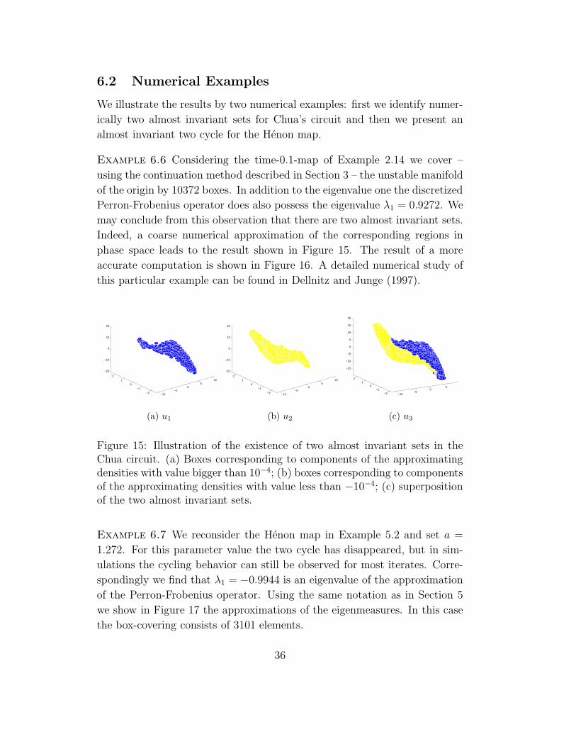
Example 6.6 Considering the time-0.1-map of Example 2.14 we cover –
using the continuation method described in Section 3 – the unstable manifold
of the origin by 10372 boxes. In addition to the eigenvalue one the discretized
Perron-Frobenius operator does also possess the eigenvalue λ1 = 0.9272. We
may conclude from this observation that there are two almost invariant sets.
Indeed, a coarse numerical approximation of the corresponding regions in
phase space leads to the result shown in Figure 15. The result of a more
accurate computation is shown in Figure 16. A detailed numerical study of
this particular example can be found in Dellnitz and Junge (1997).
−10−5
05
10
−2
−1
0
1
2
−20
−10
0
10
20
(a) u1
−10−5
05
10
−2
−1
0
1
2
−20
−10
0
10
20
(b) u2
−10−5
05
−2−1
01
2
−15
−10
−5
0
5
10
15
20
(c) u3
Figure 15: Illustration of the existence of two almost invariant sets in theChua circuit. (a) Boxes corresponding to components of the approximatingdensities with value bigger than 10−4; (b) boxes corresponding to componentsof the approximating densities with value less than −10−4; (c) superpositionof the two almost invariant sets.
Example 6.7 We reconsider the Henon map in Example 5.2 and set a =
1.272. For this parameter value the two cycle has disappeared, but in sim-
ulations the cycling behavior can still be observed for most iterates. Corre-
spondingly we find that λ1 = −0.9944 is an eigenvalue of the approximation
of the Perron-Frobenius operator. Using the same notation as in Section 5
we show in Figure 17 the approximations of the eigenmeasures. In this case
the box-covering consists of 3101 elements.
36
Figure 16: Two almost invariant sets for Chua’s circuit.
7 Adaptive Subdivision Strategies
The standard subdivision algorithm may approximate a part of the global
attractor which is dynamically irrelevant in the sense that no invariant mea-
sure has support on this subset. The reason is that each box is subdivided
in a step of the subdivision algorithm regardless of any information on the
dynamical behavior. In particular, also those subsets of the relative global
attractor corresponding to unstable or transient dynamical behavior are ap-
proximated by the standard procedure.
On the other hand, if one is mainly interested in the approximation of
the support of the (natural) invariant measure rather than in the precise
geometric structure of the global attractor then this strategy may lead to
unnecessary high storage and computation requirements. In the following
we present a modified subdivision strategy (see Dellnitz and Junge (1998))
which avoids this drawback: roughly speaking,
– in the subdivision step we use the information on the actual approxi-
mation of the invariant measure to decide whether or not a box should
be subdivided;
– in the selection step we keep only those boxes which have a nonempty
intersection with the support of the invariant measure.
37
−1−0.5
00.5
11.5
−1
−0.5
0
0.5
1
1.50
0.5
1
1.5
2
2.5
x 10−3
xy
v0
(a) v0
−1−0.5
00.5
11.5
−1
−0.5
0
0.5
1
1.5
−2
−1
0
1
2
x 10−3
xy
v1
(b) v1
−1−0.5
00.5
11.5
−1
−0.5
0
0.5
1
1.5−1
0
1
2
3
4
5
x 10−3
xy
u0
(c) u0
−1−0.5
00.5
11.5
−1
−0.5
0
0.5
1
1.5−1
0
1
2
3
4
5
x 10−3
xy
u1
(d) u1
Figure 17: Eigenvectors v0, v1 of the approximation of the Perron-Frobeniusoperator and approximations u0, u1 of probability measures which correspondto the two components of the almost 2-cycle for the Henon map (a = 1.272,b = 0.2).
7.1 Adaptive Subdivision Algorithm
Let (δk) be a sequence of positive real numbers such that δk → 0 for k → ∞.
The algorithm generates a sequence of pairs
(B0, u0), (B1, u1), (B2, u2), . . .
where the Bk’s are finite collections of compact subsets of Rn and the discrete
measures uk : Bk → [0, 1] can be interpreted as approximations to an SRB-
measure µSRB:
uk(B) ≈ µSRB(B) for all B ∈ Bk.
38
Given an initial pair (B0, u0), one inductively obtains (Bk, uk) from (Bk−1, uk−1)
for k = 1, 2, . . . in three steps:
(i) Subdivision: Define
B+k−1 = {B ∈ Bk−1 : uk−1(B) ≥ δk−1}.
Construct a new (sub-)collection B+k such that
⋃
B∈B+k
B =⋃
B∈B+k−1
B and diam(B+k ) ≤ θ diam(B+
k−1)
for some 0 < θ < 1.
(ii) Selection: Set Bk =(Bk−1\B
+k−1
)∪B+
k . Using the space of simple func-
tions on the collection Bk compute a fixed point uk of the discretized
Perron-Frobenius operator. Set
Bk = {B ∈ Bk : uk(B) > 0} and uk = uk|Bk.
A result on the convergence of this method has been proven in the context
of sufficiently regular stochastic transition functions, see Junge (2000) for
details.
Remarks 7.1 (a) In principle there is some freedom in choosing the se-
quence (δk) of positive numbers used in the subdivision step. Note that
this sequence determines the number of boxes which will be subdivided
and hence it has a significant influence on the storage requirement. In
the computations we used
δk =1
Nk
∑
B∈Bk
uk(B) =1
Nk,
where Nk is the number of boxes in Bk.
(b) One can think of more sophisticated ways of choosing the subcollection
which is going to be refined in the subdivision step. In fact, one can
show that one should aim for an estimate of the local error (between
the true and the approximate invariant density) and subdivide only
those boxes for which this estimate exceeds its average. See Guder
and Kreuzer (1999) and Junge (1999) for details on these alternative
approaches.
39
7.2 Numerical Examples
In this section we illustrate the adaptive scheme by two numerical examples.
First we consider the Logistic Map again. We will see that, as expected,
the adaptive technique is particularly useful if the underlying invariant den-
sity has singularities. Additionally we consider the Henon map as a two-
dimensional example and show the box refinement produced by the adaptive
subdivision algorithm at a certain step. Again, we refer to Section 8 for
details on the numerical realization.
Example 7.2 We have approximated the density h of the unique absolutely
continuous invariant measure of the Logistic Map using
(a) piecewise constant functions on a uniform partition and
(b) the adaptive subdivision algorithm.
Figure 18 shows the L1-error between h and the approximate densities versus
the cardinality of the partitions.
100
101
102
103
104
105
106
10−5
10−4
10−3
10−2
10−1
100
number of boxes
L1 err
or
uniform partitionAdaptive Subdivision algorithm
Figure 18: L1-error between h and the approximate invariant densities versusthe cardinality of the underlying partitions
40
A more detailed analysis of this example using the adaptive algorithm
can be found in Murray (1998).
Example 7.3 We apply the adaptive subdivision algorithm to the Henon
map, see Example 2.13. In the computations we have chosen the parameters
a = 1.2, b = 0.2, and considered the outer box B0 = {[−2, 2]2}.
In Figure 19 we present a tiling of the square [−2, 2]2 obtained by the
adaptive subdivision algorithm after several subdivision steps. The resulting
box-collection B consists of the grey boxes shown in part (a) of this figure.
We expect that due to the numerical approximation some boxes have posi-
tive discrete measure although they do not intersect the support of the real
natural invariant measure. Having this in mind we neglect those boxes with
very small discrete measure and show in Figure 19(b) a subcollection B ⊂ B
with the property that ∑
B∈B
u(B) ≈ 0.99 (7.1)
(see also Remark 7.1(b)). An approximation of a (natural) invariant measure
obtained by the adaptive subdivision algorithm is shown in Figure 20.
Remark 7.4 For the choice of the parameter values we cannot explicitly
write down a natural invariant measure. Hence it is impossible to compare
the numerical results using analytical ones. Moreover, it is not even known for
an arbitrary choice of parameter values whether or not the Henon map pos-
sesses an SRB-measure. However, as already mentioned before, M. Benedicks
and L.-S. Young proved that the Henon map indeed has an SRB-measure for
a “large” set of parameter values, see Benedicks and Young (1993).
8 Implementational Details
In this Section we are describing the details of the implementation of the
set oriented algorithms. All of the algorithms described in this chapter have
been implemented in the software package GAIO which can be obtained from
the authors.
41
−2 −1.5 −1 −0.5 0 0.5 1 1.5 2−2
−1.5
−1
−0.5
0
0.5
1
1.5
2
x
y
(a)
−0.8 −0.6 −0.4 −0.2 0 0.2 0.4 0.6 0.8 1 1.2−0.8
−0.6
−0.4
−0.2
0
0.2
0.4
0.6
0.8
1
1.2
x
y
(b)
Figure 19: (a) A tiling of the square [−2, 2]2 obtained by the adaptive subdi-vision algorithm; and (b) the subcollection B of boxes with discrete densitybigger than 0.35 (see also (7.1)).
−2−1
01
2
−2
−1
0
1
20
50
100
150
200
xy
dens
ity
Figure 20: Illustration of a (natural) invariant measure for the Henon map.The picture shows the density of the discrete measure on B, see (7.1).
8.1 Realization of the Collections and the Subdivision
Step
We realize the closed subsets constituting the collections using generalized
rectangles (“boxes”) of the form
B(c, r) = {y ∈ Rn : |yi − ci| ≤ ri for i = 1, . . . , n} ,
42
where c, r ∈ Rn, ri > 0 for i = 1, . . . , n, are the center and the radius
respectively. In the k-th subdivision step we subdivide each rectangle B(c, r)
of the current collection by bisection with respect to the j-th coordinate,
where j is varied cyclically, that is, j = ((k − 1) mod n) + 1. This division
leads to two rectangles B−(c−, r) and B+(c+, r), where
ri =
{ri for i 6= jri/2 for i = j
, c±i =
{ci for i 6= j
ci ± ri/2 for i = j.
Starting with a single initial rectangle we perform the subdivision until a
prescribed size σ of the diameter relative to the initial rectangle is reached.
The collections constructed in this way can easily be stored in a binary
tree. In Figure 21 we show the representation of three subdivision steps
in three dimensions (n = 3) together with the corresponding sets Qk, k =
0, 1, 2, 3, see (2.6). Note that each collection and the corresponding covering
Qk are completely determined by the tree structure and the initial rectangle
B(c, r).
Root
0 1
00 01
000 001 010
10
100 101
Figure 21: Storage scheme for the collections and the corresponding coveringsQk, k = 0, 1, 2, 3.
8.2 Realization of the Intersection Test
In the subdivision algorithms as well as in the continuation method we have
to decide whether for a given collection Bk the image of a set B ∈ Bk has a
nonzero intersection with another set B′ ∈ Bk, i.e. whether
f(B) ∩B′ = ∅. (8.1)
In simple model problems such as our trivial Example 2.5 this decision can
be made analytically. For more complex problems we have to use some kind
43
of discretization. Motivated by similar approaches in the context of cell-
mapping techniques (see Hsu (1992)), we choose a finite set of test points in
each set B ∈ Bk and replace the condition (8.1) by
f(x) 6∈ B′ for all test points x ∈ B . (8.2)
Obviously, it may still occur that f(B) ∩ B′ is nonempty although (8.2) is
valid.
Distribution of Test Points
It remains to discuss how the test points are distributed inside each rectan-
gle. To define the test points, observe that R(c, r) is the affine image of the
standard cube [−1, 1]n scaled by r and translated by c. Using this transfor-
mation it is sufficient to define the test points for the standard cube. Simple
geometric considerations make it clear that one should obtain the best results
for the test in (8.2) if most of the test points are lying on the boundary of the
rectangle. An efficient choice for problems of dimension up to three turned
out to be N test points on each edge distributed according to
t(`) =2`− 1
N− 1 for ` = 1, ..., N (8.3)
on [−1, 1]. As an additional test point we choose the center c = 0. Since an
n-dimensional rectangle has n2n−1 edges, we end up with p = Nn2n−1 + 1
test points per box.
Rigorous Choice of Test Points
The numerical realization of the intersection test can be made rigorous in
the sense that no boxes are lost due to the discretization. Indeed, to accom-
plish this it is sufficient to have estimates for the Lipschitz constants of the
dynamical system f on Q.
To be more precise let B be a collection of boxes B = B(c, r) = {x :
|x− c| ≤ r} (where we write |x| = (|x1|, . . . , |xn|) and x ≤ y for x, y ∈ Rn, if
xi ≤ yi for i = 1, . . . , n). We need to compute the set-wise image
F(B) = {B′ ∈ B | f(B) ∩ B′ 6= ∅},
for every B ∈ B. Our goal here is to construct a set F(B) of boxes for which
F(B) ⊂ F(B),
44
so that we get a rigorous covering of f(B). To this end we will need to know
local Lipschitz constants for f , that is, we require that for every box B in
the current collection there is a nonnegative matrix L = L(B) ∈ Rn×n such
that
|f(y) − f(x)| ≤ L|y − x| (8.4)
for x, y ∈ B. If f is continuously differentiable then Lij = maxξ∈B |∂jfi(ξ)|.
Now let h = h(B) ∈ Rn be a positive vector such that
Lh ≤ 2r.
Using the mesh widths h we now define a mesh
T = T (B) = {x : (xi − ci) ∈ hiZ, i = 1, . . . , n}.
It is easy to see that for every y ∈ B there is a meshpoint x ∈ T (B), such
that |y − x| ≤ h/2. On the other hand we are interested in a finite set of
test points and indeed the only points x ∈ T (B) we really need are those for
which there is actually a y ∈ B with |y − x| ≤ h/2. So let
T (B) = T (B) ∩ {x | B ∩ int B(x, h/2) 6= ∅}
be the set of test points. Note that an additional constraint on h will be
necessary in order to ensure that the test points are contained in B, which is
necessary, since the local Lipschitz-estimate (8.4) on f is only valid for points
in B. Finally we construct the collection F(B) by setting
F(B) = {B ∈ B | B ∩ B(f(x), r) 6= ∅ for some x ∈ T (B)}. (8.5)
x
B
f(x)
B(f(x),r)
f(B)
Figure 22: On the construction of F(B).
The idea of this construction is to look at the boxes B(f(x), r) 6∈ B
corresponding to the images of the test points x and to collect in F(B) all
45
boxes which have nonempty intersection with those boxes, see Figure 22. It
is important to note that the construction of F(B) is a finite task: since the
boxes B(f(x), r), x ∈ T , have the same radius as the boxes in the collections
B, it suffices to consider the vertices of B(f(x), r).
Adaptive Choice of Test Points
In order to reduce the numerical effort of the set oriented algorithms one has
to reduce the number of test points per box as far as possible. We now show
how to do that by considering local expansion rates of the map f . To this
end we consider the singular value decomposition
Df(x) = U(x)S(x)V T(x)
of Df(x), where U(x) = [u1(x), . . . , un(x)] and V (x) = [v1(x), . . . , vn(x)] are
real orthogonal (n×n)-matrices and S(x) ∈ Rn×n is a diagonal matrix having
the singular values σ1(x) ≥ · · · ≥ σn(x) of Df(x) on the diagonal.
The idea for an improved choice of the test points is to construct a mesh
with respect to the basis of right singular vectors v1(c), . . . , vn(c) of Df(c) =
U(c)S(c)V T(c) (where c denotes the center of the box under consideration)
and to choose the mesh width hi, i = 1, . . . , n in relation to the singular value
σi(c). Let us suppose for the moment that for a box B the derivative Df(x) =
Df(c) = Df = USV T is constant on a sufficiently large neighborhood ∆(B)
of B. Then
f(x) − f(y) = Df · (x− y) = USV T(x− y),
so that
|f(x) − f(y)| ≤ |U |S|V T (x− y)|
where |U | = (|uij|). We choose mesh widths h ∈ Rn, h > 0, such that
|U |Sh ≤ 2r (8.6)
and define the mesh
T = T (B) = {x : (V T (x− c))i ∈ hiZ, i = 1, . . . , n}. (8.7)
Again it is easy to see that for every y ∈ B there is a mesh point x ∈ T (B),
such that |V T (y − x)| ≤ h/2. We have to restrict ourselves to a finite set of
test points again which can be written down as
T = T (B) = T (B) ∩ {x : B ∩ int (V B(0, h/2) + x) 6= ∅} . (8.8)
46
We construct F(B) as in (8.5) and get that F(B) ⊂ F(B). Finally let us
consider the general case where Df(x) is not constant on a box. Let
M(x) = (mij(x))i,j=1,...,n = Df(x)V (c)
and set
M = (mij)i,j=1,...,n , mij = maxx∈∆(B)
|mij(x)|,
where ∆(B) is a sufficiently large neighborhood of B which we suppose to
be convex in this case. We choose mesh widths h > 0 such that
Mh ≤ 2r, (8.9)
and use the mesh as defined by (8.7) as well as the construction (8.5) for
F(B).
It can easily be shown that the union of boxes in F(B) covers f(B), i.e.
F(B) ⊂ F(B),
see Junge (1999) for details.
8.3 Implementation of the Measure Computation
The feasibility of the computation of invariant measures even for higher di-
mensional systems relies on the fact that we first compute an outer covering
B of the underlying invariant set by one of the set oriented methods presented
in this chapter.
As the ansatz spaces Vd for the discretization of the Perron-Frobenius
operator we use the spaces of simple functions on the given collection B. It
is easy to see that the discretized Perron-Frobenius operator is then given by
a stochastic matrix P = (pij) with entries
pij =m(f−1(Bi) ∩Bj)
m(Bj), Bi, Bj ∈ B.
For the computation of the pij’s we either use a Monte-Carlo approach (see
Hunt (1994)) or an exhaustion technique as described in Guder et al. (1997).
The latter method is particularly useful when local Lipschitz constants are
available for the underlying dynamical system.
For the computation of certain eigenvectors of the resulting (sparse) ma-
trix P an Arnoldi method is used (see Lehoucq et al. (1998)).
47
Acknowledgments Figures 4, 6, 7, 9 and 16 have been produced using
the software platform GRAPE, see Rumpf and Wierse (1992).
References
M. Benedicks and L.-S. Young. Sinai-Bowen-Ruelle measures for certain Henonmaps. Invent. math., 112:541–576, 1993.
M. Blank and G. Keller. Random perturbations of chaotic dynamical systems.stability of the spectrum. Nonlinearity, 11(5):1351–1364, 1998.
R. Bowen and D. Ruelle. The ergodic theory of axiom a flows. Invent. math., 29:181–202, 1975.
P. Chossat and M. Golubitsky. Symmetry-increasing bifurcation of chaotic attrac-tors. Physica D, 32:423–436, 1988.
C. Conley. Isolated invariant sets and the Morse index. American MathematicalSociety, 1978.
M. Dellnitz, G. Froyland, and St. Sertl. On the isolated spectrum of the Perron-Frobenius operator. To appear in Nonlinearity, 2000a.
M. Dellnitz and A. Hohmann. The computation of unstable manifolds using subdi-vision and continuation. In H.W. Broer, S.A. van Gils, I. Hoveijn, and F. Takens,editors, Nonlinear Dynamical Systems and Chaos, pages 449–459. Birkhauser,PNLDE 19, 1996.
M. Dellnitz and A. Hohmann. A subdivision algorithm for the computation ofunstable manifolds and global attractors. Num. Math., 75:293–317, 1997.
M. Dellnitz and O. Junge. Almost invariant sets in Chua’s circuit. Int. J. Bif. andChaos, 7(11):2475–2485, 1997.
M. Dellnitz and O. Junge. An adaptive subdivision technique for the approxi-mation of attractors and invariant measures. Comput. Visual. Sci., 1:63–68,1998.
M. Dellnitz and O. Junge. On the approximation of complicated dynamical be-havior. SIAM J. Numer. Anal., 36(2):491–515, 1999.
M. Dellnitz, O. Junge, M. Rumpf, and R. Strzodka. The computation of anunstable invariant set inside a cylinder containing a knotted flow. In Proceedingsof Equadiff ’99, Berlin, 2000b.
M. Dellnitz, O. Schutze, and St. Sertl. Finding zeros by multilevel subdivisiontechniques. Submitted to IMA Journal of Numerical Analysis, 2000c.
P. Deuflhard, M. Dellnitz, O. Junge, and Ch. Schutte. Computation of essentialmolecular dynamics by subdivision techniques I: basic concept. In P. Deuflhard,J. Hermans, B. Leimkuhler, A.E. Mark, S. Reich, and R.D. Skeel, editors, Com-putational Molecular Dynamics: Challenges, Methods, Ideas., volume 4 of Lec-ture Notes in Computational Science and Engineering, pages 98–115. Springer,1998.
48
P. Deuflhard, W. Huisinga, A. Fischer, and Ch. Schutte. Identification of almostinvariant aggregates in reversible nearly uncoupled Markov chains. Linear Al-gebra and its Applications, 315:39–59, 2000.
J. Ding, Q. Du, and T. Y. Li. High order approximation of the Frobenius-Perronoperator. Appl. Math. Comp., 53:151–171, 1993.
J. Ding and A. Zhou. Finite approximations of Frobenius-Perron operators. Asolution of Ulam’s conjecture to multi-dimensional transformations. Physica D,1-2:61–68, 1996.
J. R. Dormand and P. J. Prince. Higher order embedded runge-kutta formulae. J.Comp. Appl. Math., 7:67–75, 1981.
M. Eidenschink. Exploring Global Dynamics: A Numerical Algorithm Based onthe Conley Index Theory. PhD Thesis, Georgia Institute of Technology, 1995.
G. Froyland. Estimating Physical Invariant Measures and Space Averages of Dy-namical Systems Indicators. PhD thesis, University of Western Australia, 1996.
G. Keller. Stochastic stability in some chaotic dynamical systems. Monatsh. Math.,94:313–333, 1982.
J. Guckenheimer and Ph. Holmes. Nonlinear Oscillations, Dynamical Systems,and Bifurcations of Vector Fields. Springer, 1983.
R. Guder, M. Dellnitz, and E. Kreuzer. An adaptive method for the approximationof the generalized cell mapping. Chaos, Solitons and Fractals, 8(4):525–534,1997.
R. Guder and E. Kreuzer. Control of an adaptive refinement technique of gener-alized cell mapping by system dynamics. J. Nonl. Dyn., 20(1):21–32, 1999.
H. Hsu. Global analysis by cell mapping. Int. J. Bif. Chaos, 2:727–771, 1992.
Fern Y. Hunt. A Monte Carlo approach to the approximation of invariant measures.Random & Computational Dynamics, 2(1):111–133, 1994.
O. Junge. Mengenorientierte Methoden zur numerischen Analyse dynamischerSysteme. PhD thesis, University of Paderborn, 1999.
O. Junge. An adaptive subdivision technique for the approximation of attractorsand invariant measures. Part II: Proof of convergence. Submitted, 2000.
H. Keller and G. Ochs. Numerical approximation of random attractors. In Stochas-tic dynamics, pages 93–115. Springer, 1999.
Yu. Kifer. General random perturbations of hyperbolic and expanding transfor-mations. J. Analyse Math., 47:111–150, 1986.
E. Kreuzer. Numerische Untersuchung nichtlinearer dynamischer Systeme.Springer, 1987.
A. Lasota and M.C. Mackey. Chaos, Fractals and Noise. Springer, 1994.
49
A. Lasota and J.A. Yorke. On the existence of invariant measures for piecewisemonotonic transformations. Transactions of the AMS, 186:481–488, 1973.
R. B. Lehoucq, D. C. Sorensen, and C. Yang. ARPACK users’ guide. Soci-ety for Industrial and Applied Mathematics (SIAM), Philadelphia, PA, 1998.ISBN 0-89871-407-9. Solution of large-scale eigenvalue problems with implicitlyrestarted Arnoldi methods.
T.-Y. Li. Finite approximation for the Frobenius-Perron operator. A solution toUlam’s conjecture. J. Approx. Theory, 17:177–186, 1976.
K. Mehlhorn. Data Structures and Algorithms. Springer, 1984.
R. Murray. Adaptive approximation of invariant measures. Preprint, 1998.
G. Osipenko. Construction of attractors and filtrations. In K. Mischaikow,M. Mrozek, and P. Zgliczynski, editors, Conley Index Theory, pages 173–191.Banach Center Publications 47, 1999.
D. Ruelle. A measure associated with axiom a attractors. Amer. J. Math., 98:619–654, 1976.
M. Rumpf and A. Wierse. GRAPE, eine objektorientierte Visualisierungs– undNumerikplattform. Informatik, Forschung und Entwicklung, 7:145–151, 1992.
Ch. Schutte. Conformational Dynamics: Modelling, Theory, Algorithm, and Ap-plication to Biomolecules. Habilitation thesis, Freie Universitat Berlin, 1999.
M. Shub. Global stability of dynamical systems. Springer, 1987.