20
Shock focusing and Converging Geometries - in the context of the VTF validation D.J.Hill Galcit Nov 1, 2005
| Date post: | 21-Dec-2015 |
| Category: |
Documents |
| View: | 216 times |
| Download: | 0 times |
Shock focusing and Converging Geometries - in the context of the VTF validation
D.J.Hill
GalcitNov 1, 2005
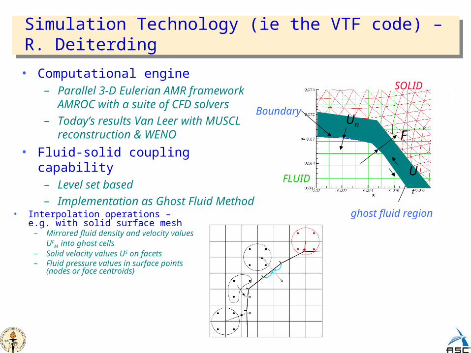
Simulation Technology (ie the VTF code) – R. Deiterding
• Computational engine– Parallel 3-D Eulerian AMR framework
AMROC with a suite of CFD solvers
– Today’s results Van Leer with MUSCL reconstruction & WENO
• Fluid-solid coupling capability– Level set based
– Implementation as Ghost Fluid Method
ghost fluid region
FLUID
SOLID
Boundary
F
U
t
Un
• Interpolation operations – e.g. with solid surface mesh
– Mirrored fluid density and velocity values UF
M into ghost cells – Solid velocity values US on facets– Fluid pressure values in surface points
(nodes or face centroids)

Non-symmetric external wedge
An Example of Shocks -complex boundaries and Richtmyer-Meshkov Instability
• Mach 1.5 shock in Air interacts with a non-symmetric wedge
• Followed by an SF6 interface
• Temperature plots with density shadows
amroc/weno/applications/euler/2d/Triangle/

Existing Experiments: Conical Geometry
– Setchel,Strom,Sturtevant -1972• 10 degree half angle.
• Argon at 1.5 Torr
• Mach 6 shock
– Milton, Takayama -1998, Milton et al -1986• 10,20,30 degree half angle
• Mach 2.4, gamma 1.4
– Kumar, Hornug, Sturtevant – 2003• Air-SF6, Mach 1.55
• Perturbed interface – RMI.
Similar to “Phase 0” - one gas only
Two gases with perturbed interface
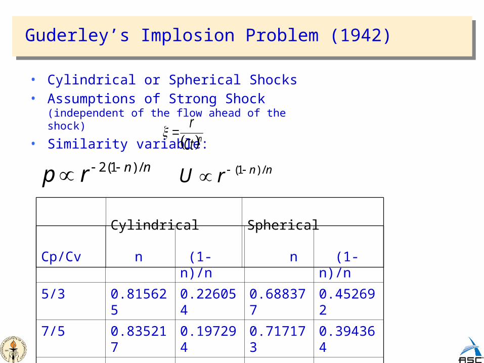
Guderley’s Implosion Problem (1942)
• Cylindrical or Spherical Shocks• Assumptions of Strong Shock (independent of the
flow ahead of the shock)
• Similarity variable:
Cp/Cv n (1-n)/n n (1-n)/n
5/3 0.815625 0.226054 0.688377 0.452692
7/5 0.835217 0.197294 0.717173 0.394364
6/5 0.861163 0.161220 0.757142 0.320756
Cylindrical Spherical
nnrp /)1(2 nnrU /)1(
nCt
r

Simulation configuration for Conical shocktube: SSS ‘72
• Mach 6 shock• Argon (gamma = 5/3,
molecular weight 39.9)
• 10.17 degree half angle
• Aperture diameter 15.3 cm
• Probe width 3.22 mm
• Simulations used analytic levelset with the GFM capability of the VTF
Vtf/amroc/clawpack/applications/euler/2d/Conical_Shocktube/ And Vtf/amroc/clawpack/applications/euler/3d/Conical_Shocktube/
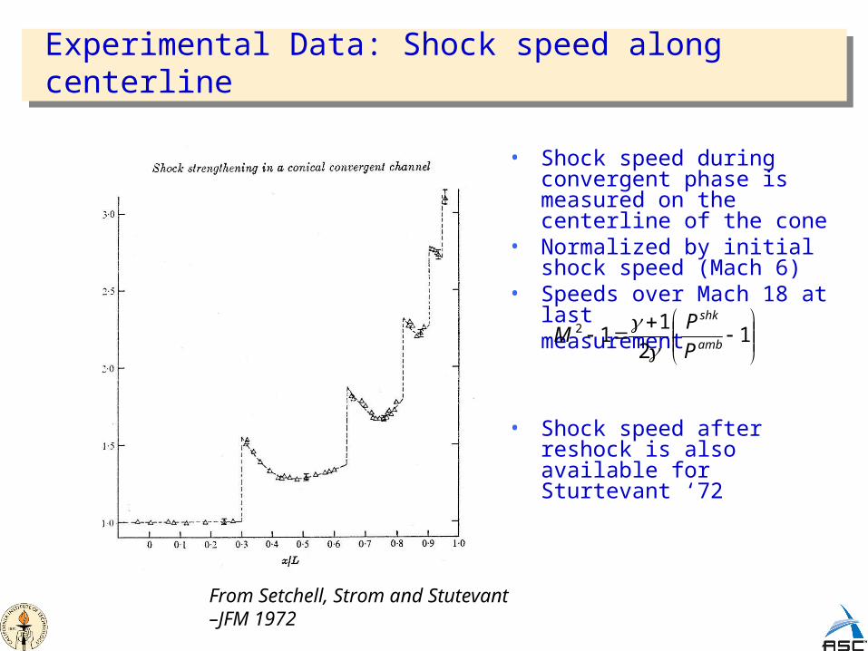
Experimental Data: Shock speed along centerline
• Shock speed during convergent phase is measured on the centerline of the cone
• Normalized by initial shock speed (Mach 6)
• Speeds over Mach 18 at lastmeasurement
• Shock speed after reshock is also available for Sturtevant ‘72
From Setchell, Strom and Stutevant –JFM 1972
1
2
112
amb
shk
P
PM

Shock diagram in conical geometry
SSS – JFM 1972
Jumps in shock speed correspond to Machstem collisions on the axis of symmetry
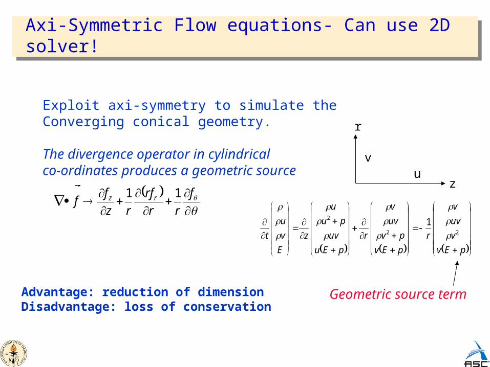
Axi-Symmetric Flow equations- Can use 2D solver!
pEv
v
uv
v
r
pEv
pv
uv
v
r
pEu
uv
pu
u
z
E
v
u
t 22
2 1
vu
z
r
Geometric source term
f
rr
rf
rz
ff rz 11
Exploit axi-symmetry to simulate theConverging conical geometry.
The divergence operator in cylindrical co-ordinates produces a geometric source
Advantage: reduction of dimensionDisadvantage: loss of conservation
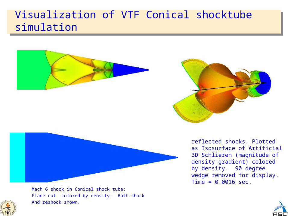
Visualization of VTF Conical shocktube simulation
Leading shock (blue) and reflected shocks. Plotted as Isosurface of Artificial 3D Schlieren (magnitude of density gradient) colored by density. 90 degree wedge removed for display. Time = 0.0016 sec.
Mach 6 shock in Conical shock tube:Plane cut colored by density. Both shock And reshock shown.
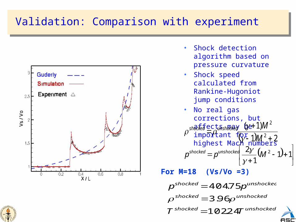
Validation: Comparison with experiment
• Shock detection algorithm based on pressure curvature
• Shock speed calculated from Rankine-Hugoniot jump conditions
• No real gas corrections, but affects may be important for highest Mach numbers
21
)1(2
2
M
Munshockedshocked
11
1
2 2Mpp unshockedshocked
For M=18 (Vs/Vo =3)
unshockedshocked
unshockedshocked
unshockedshocked
TT
pp
24.102
96.3
75.404
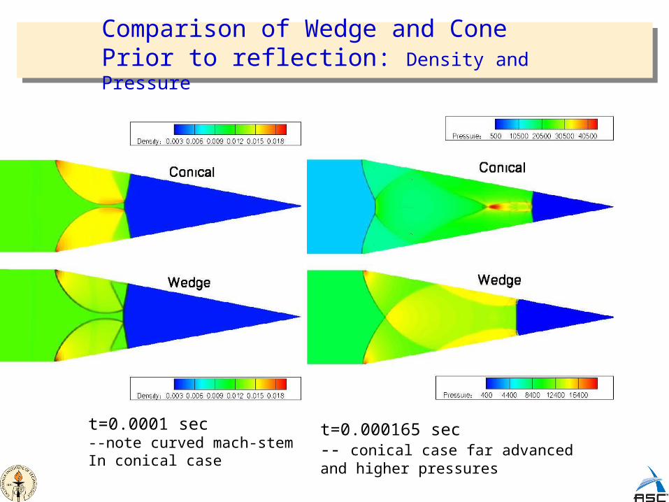
Comparison of Wedge and ConePrior to reflection: Density and Pressure
t=0.0001 sec--note curved mach-stemIn conical case
t=0.000165 sec-- conical case far advancedand higher pressures
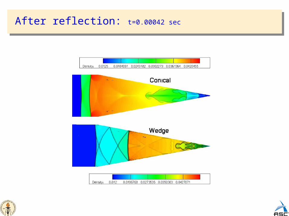
After reflection: t=0.00042 sec

ASC converging shock experiments (P. Dimotakis)
• Phase 0: A single gas is used, the shock interacts with the boundary of the wedge producing shock mach stems, reflected shocks and triple points. The focusing of the shock is achieved by the successive reflection of the shock
• Phase 1: Two gases are used. The driver gas in the shocktube, and a lens gas in the wedge. The shape of the boundary (contact) between the two gases has been specially designed to curve the shock producing a circular shock centered on the apex of the wedge. P. Dimotakis & R. Samtaney
• Phase 2: A third gas is used. It is placed within the wedge after the lens. Purturbations on the contact between this gas and the lens gas will give rise to a Richtmyer-Meshkov instability, and the acceleration towards the apex will also have aspects of the Rayleigh-Taylor instability
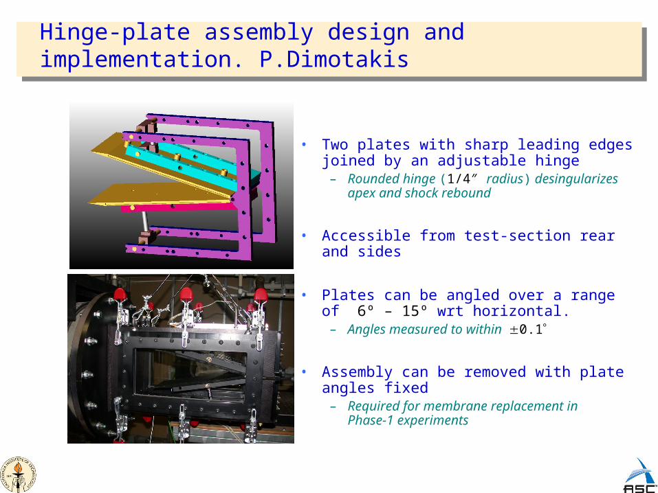
Hinge-plate assembly design and implementation. P.Dimotakis
• Two plates with sharp leading edges joined by an adjustable hinge
– Rounded hinge (1/4″ radius) desingularizes apex and shock rebound
• Accessible from test-section rear and sides
• Plates can be angled over a range of 6º – 15º wrt horizontal.
– Angles measured to within 0.1
• Assembly can be removed with plate angles fixed
– Required for membrane replacement inPhase-1 experiments
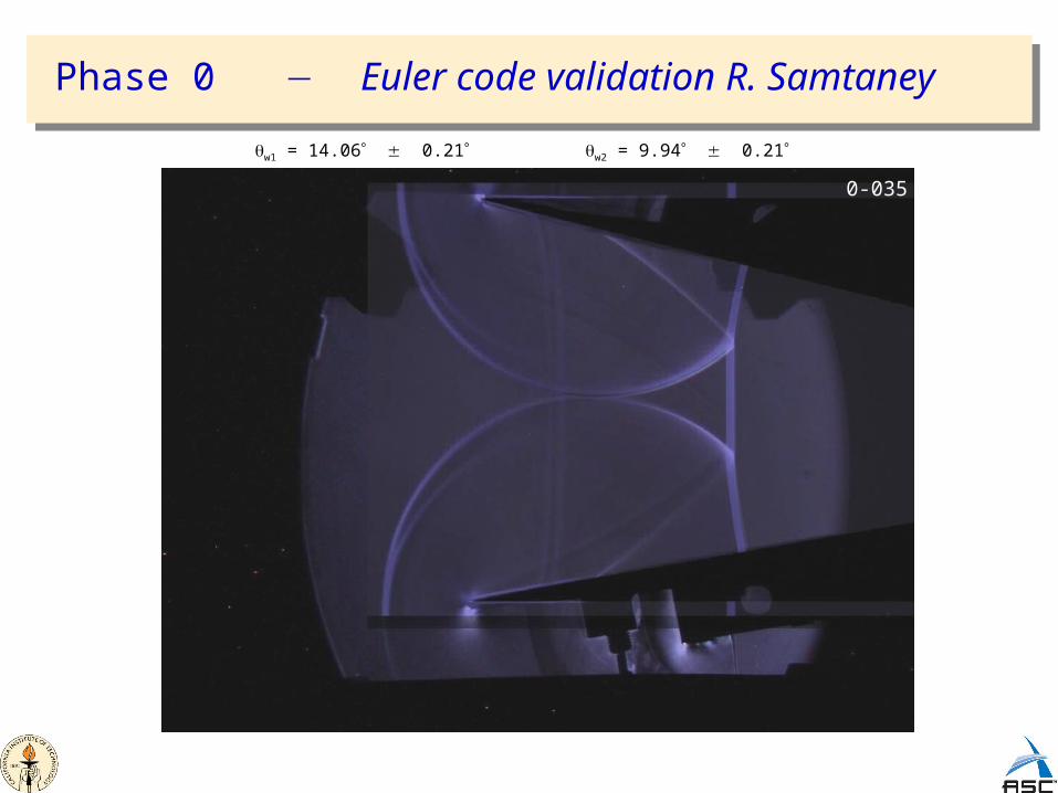
Phase 0 Euler code validation R. Samtaney
0-035
w1 = 14.06 0.21 w2 = 9.94 0.21
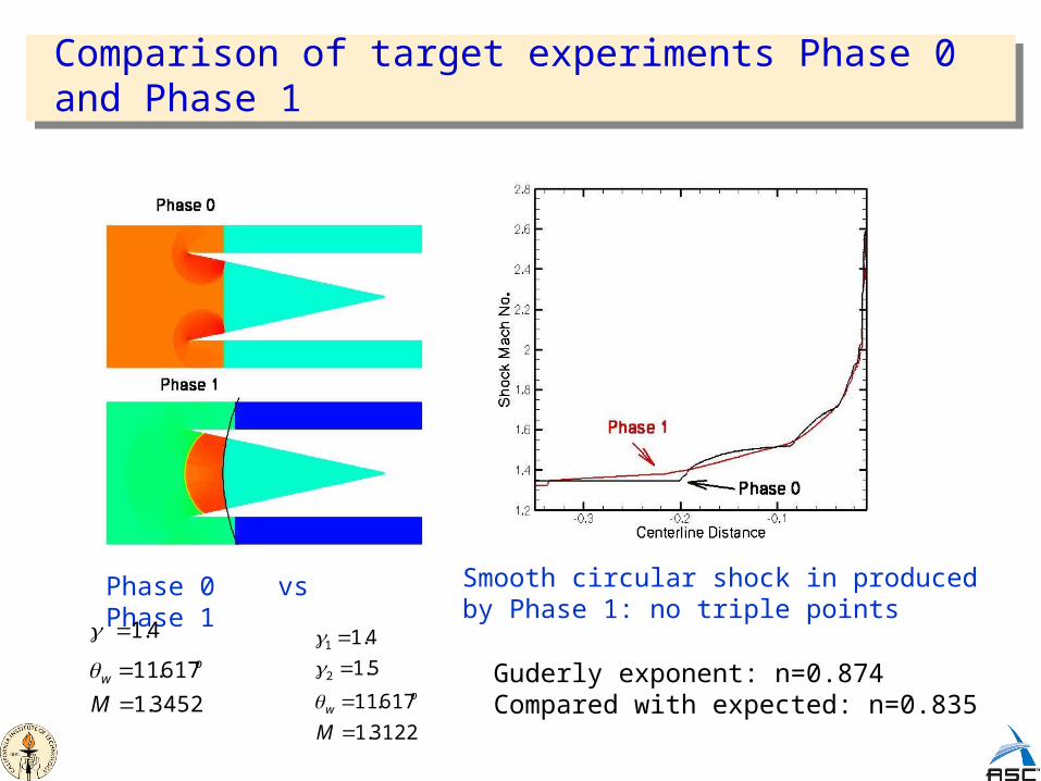
Comparison of target experiments Phase 0 and Phase 1
4.1
5.1
2
1
ow 617.11
3122.1
617.11
5.1
4.1
2
1
M
ow
Phase 0 vs Phase 1
3452.1
617.11
4.1
M
ow
Smooth circular shock in produced by Phase 1: no triple points
Guderly exponent: n=0.874Compared with expected: n=0.835
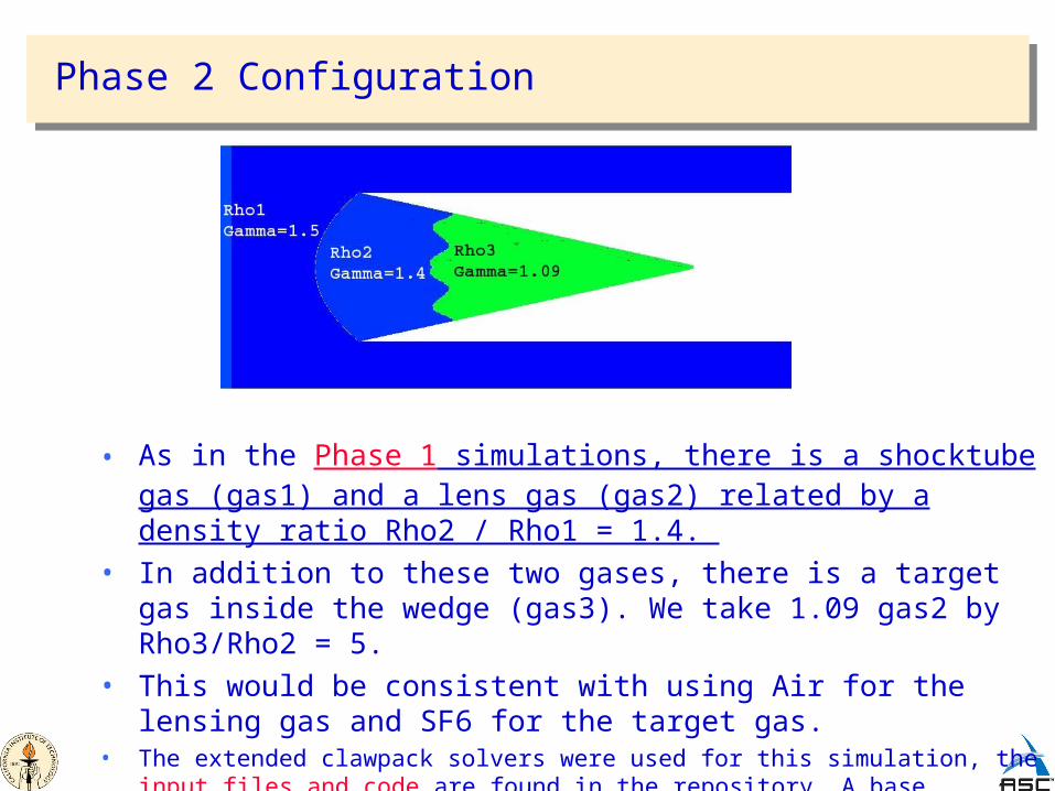
Phase 2 Configuration
• As in the Phase 1 simulations, there is a shocktube gas (gas1) and a lens gas (gas2) related by a density ratio Rho2 / Rho1 = 1.4.
• In addition to these two gases, there is a target gas inside the wedge (gas3). We take 1.09 gas2 by Rho3/Rho2 = 5.
• This would be consistent with using Air for the lensing gas and SF6 for the target gas.
• The extended clawpack solvers were used for this simulation, the input files and code are found in the repository. A base resolution of 250x100 was used with 4 additional levels of refinement (factors 2,2,2,2).
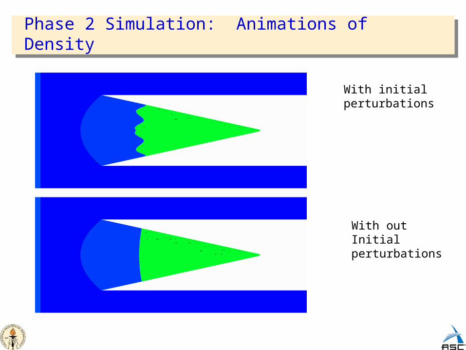
Phase 2 Simulation: Animations of Density
With initial perturbations
With outInitial perturbations
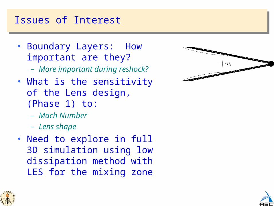
Issues of Interest
• Boundary Layers: How important are they? – More important during reshock?
• What is the sensitivity of the Lens design, (Phase 1) to:– Mach Number
– Lens shape
• Need to explore in full 3D simulation using low dissipation method with LES for the mixing zone


