Page 1
1
Short-Run Macro Model
• Short-run macro model• Macroeconomic model that explains how
changes in spending can affect real GDP in the short run
• In the short run:• Spending depends on income• Income depends on spending
© 2010 Cengage Learning. All Rights Reserved. May not be scanned, copied or duplicated, or posted to a publicly accessible Web site, in whole or in part.
Page 2
2
Consumption Spending
• Consumption spending increases when:• Disposable income rises• Wealth rises• The interest rate falls• Households become more optimistic about
the future
© 2010 Cengage Learning. All Rights Reserved. May not be scanned, copied or duplicated, or posted to a publicly accessible Web site, in whole or in part.
Page 3
3
Figure 1: Quarterly U.S. Consumption and Disposable Income, 2000–2009
© 2010 Cengage Learning. All Rights Reserved. May not be scanned, copied or duplicated, or posted to a publicly accessible Web site, in whole or in part.
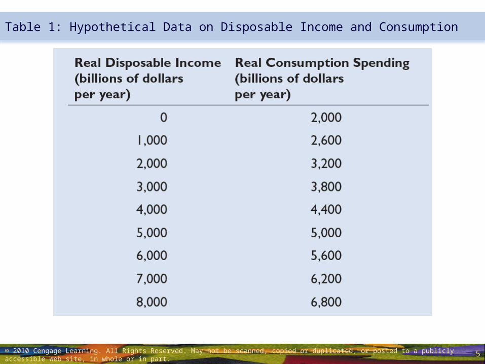
When real consumption expenditure is plotted against real disposable income, the resulting relationship is very close to linear: As real disposable income rises, so does real consumption spending
Page 4
4
Consumption Spending
• Consumption function • Positively sloped relationship • Between real consumption spending and real
disposable income• Autonomous consumption spending
• The part of consumption spending • That is independent of income• Vertical intercept of the consumption function
© 2010 Cengage Learning. All Rights Reserved. May not be scanned, copied or duplicated, or posted to a publicly accessible Web site, in whole or in part.
Page 5
5
Table 1: Hypothetical Data on Disposable Income and Consumption
© 2010 Cengage Learning. All Rights Reserved. May not be scanned, copied or duplicated, or posted to a publicly accessible Web site, in whole or in part.
Page 6
6
Figure 2: The Consumption Function
© 2010 Cengage Learning. All Rights Reserved. May not be scanned, copied or duplicated, or posted to a publicly accessible Web site, in whole or in part.
ConsumptionFunction
Real Disposable Income ($ billions)
RealConsumptionSpending($ billions)
1,000 2,000 3,000 4,000 5,000 6,000 7,000 8,000
8,000
7,000
6,000
5,000
4,000
3,000
2,000
1,000
1,000
600
ConsumptionFunction
The consumption function showsthe (linear) relationship betweenreal consumption spending andreal disposable income.
The vertical intercept ($2,000billion) is autonomousconsumption spending . . .
and the slope of the line(0.6) is the marginalpropensity to consume.
Page 7
7
Consumption Spending
• Marginal propensity to consume (MPC) is • The slope of the consumption function• The change in consumption divided by the
change in disposable income• The amount by which consumption spending
rises when disposable income rises by one dollar
0 < MPC < 1
© 2010 Cengage Learning. All Rights Reserved. May not be scanned, copied or duplicated, or posted to a publicly accessible Web site, in whole or in part.
Page 8
8
Consumption Spending
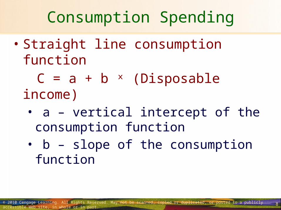
• Straight line consumption functionC = a + b ˣ (Disposable income)
• a – vertical intercept of the consumption function
• b – slope of the consumption function
© 2010 Cengage Learning. All Rights Reserved. May not be scanned, copied or duplicated, or posted to a publicly accessible Web site, in whole or in part.
Page 9
9
Consumption Spending
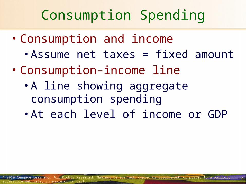
• Consumption and income• Assume net taxes = fixed amount
• Consumption–income line• A line showing aggregate consumption
spending • At each level of income or GDP
© 2010 Cengage Learning. All Rights Reserved. May not be scanned, copied or duplicated, or posted to a publicly accessible Web site, in whole or in part.
Page 10
10
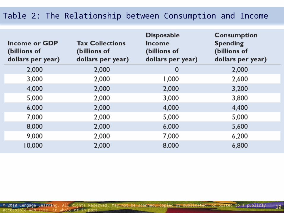
Table 2: The Relationship between Consumption and Income
© 2010 Cengage Learning. All Rights Reserved. May not be scanned, copied or duplicated, or posted to a publicly accessible Web site, in whole or in part.
Page 11
11
Figure 3: The Consumption–Income Line
© 2010 Cengage Learning. All Rights Reserved. May not be scanned, copied or duplicated, or posted to a publicly accessible Web site, in whole or in part.
Real Income ($ billions)
ConsumptionFunction
RealConsumptionSpending($ billions)
1,000 2,000 3,000 4,000 5,000 6,000 7,000 8,000 9,000
5,600
5,000
4,000
3,000
2,000
1,000
1,000
600
Consumption–Income
Line
3. but a differentvertical intercept.
2. The line has the sameslope as the consumptionfunction in Figure 2 . . .
1. To draw the consumption–income line, we measure real income (instead of real disposable income) on the horizontal axis.
B
A
Page 12
12
Consumption Spending
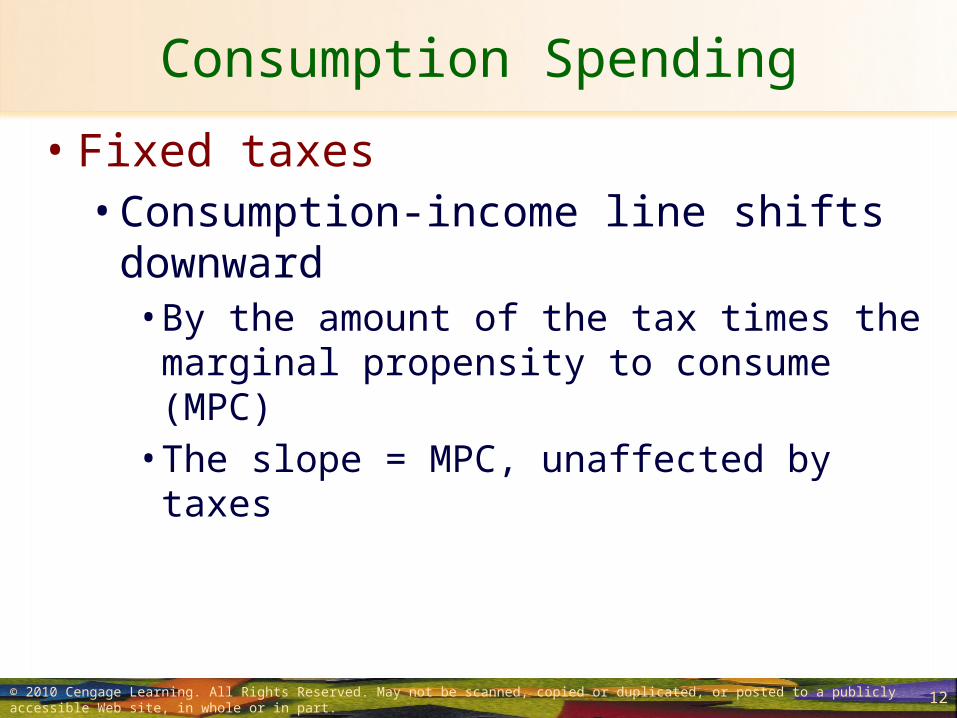
• Fixed taxes• Consumption-income line shifts downward
• By the amount of the tax times the marginal propensity to consume (MPC)
• The slope = MPC, unaffected by taxes
© 2010 Cengage Learning. All Rights Reserved. May not be scanned, copied or duplicated, or posted to a publicly accessible Web site, in whole or in part.
Page 13
13
Consumption Spending
• Income - increase• With no change in taxes• Disposable income – increase• Consumption spending – increase• Movement rightward along the
consumption-income line
© 2010 Cengage Learning. All Rights Reserved. May not be scanned, copied or duplicated, or posted to a publicly accessible Web site, in whole or in part.
Page 14
14
Consumption Spending
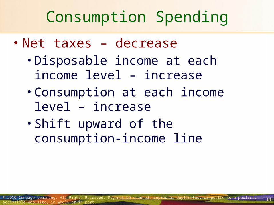
• Net taxes – decrease• Disposable income at each income level –
increase• Consumption at each income level –
increase• Shift upward of the consumption-income
line
© 2010 Cengage Learning. All Rights Reserved. May not be scanned, copied or duplicated, or posted to a publicly accessible Web site, in whole or in part.
Page 15
15
Consumption Spending
• Household wealth – increase• Autonomous consumption – increase• Consumption at each level of disposable
income – increase• Consumption spending at each level of
income – increase • Shift upward of the consumption-income
line
© 2010 Cengage Learning. All Rights Reserved. May not be scanned, copied or duplicated, or posted to a publicly accessible Web site, in whole or in part.
Page 16
16
Figure 4: A Shift in the Consumption–Income Line
© 2010 Cengage Learning. All Rights Reserved. May not be scanned, copied or duplicated, or posted to a publicly accessible Web site, in whole or in part.
Real Income ($ billions)
ConsumptionFunction
RealConsumptionSpending($ billions)
1,000 2,000 3,000 4,000 5,000 6,000 7,000 8,000 9,000
6,000
5,000
4,000
3,000
2,000
1,000
Consumption–Income LineWhen Net Taxes=$2,000 billion
Consumption–Income LineWhen Net Taxes=$500 billion
Page 17
17
Consumption Spending
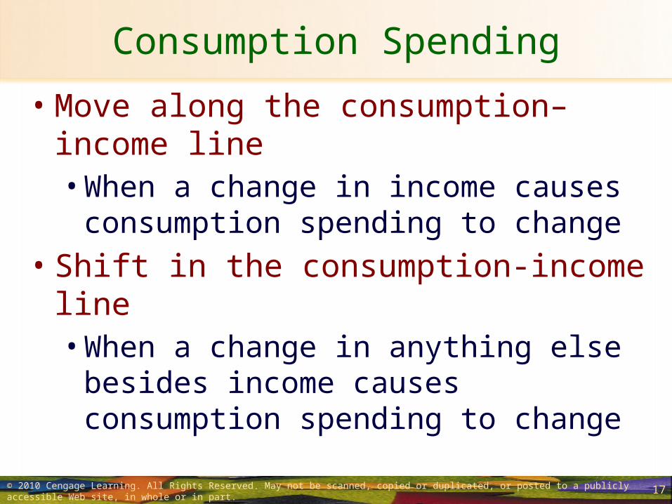
• Move along the consumption–income line • When a change in income causes
consumption spending to change• Shift in the consumption-income line
• When a change in anything else besides income causes consumption spending to change
© 2010 Cengage Learning. All Rights Reserved. May not be scanned, copied or duplicated, or posted to a publicly accessible Web site, in whole or in part.
Page 18
18
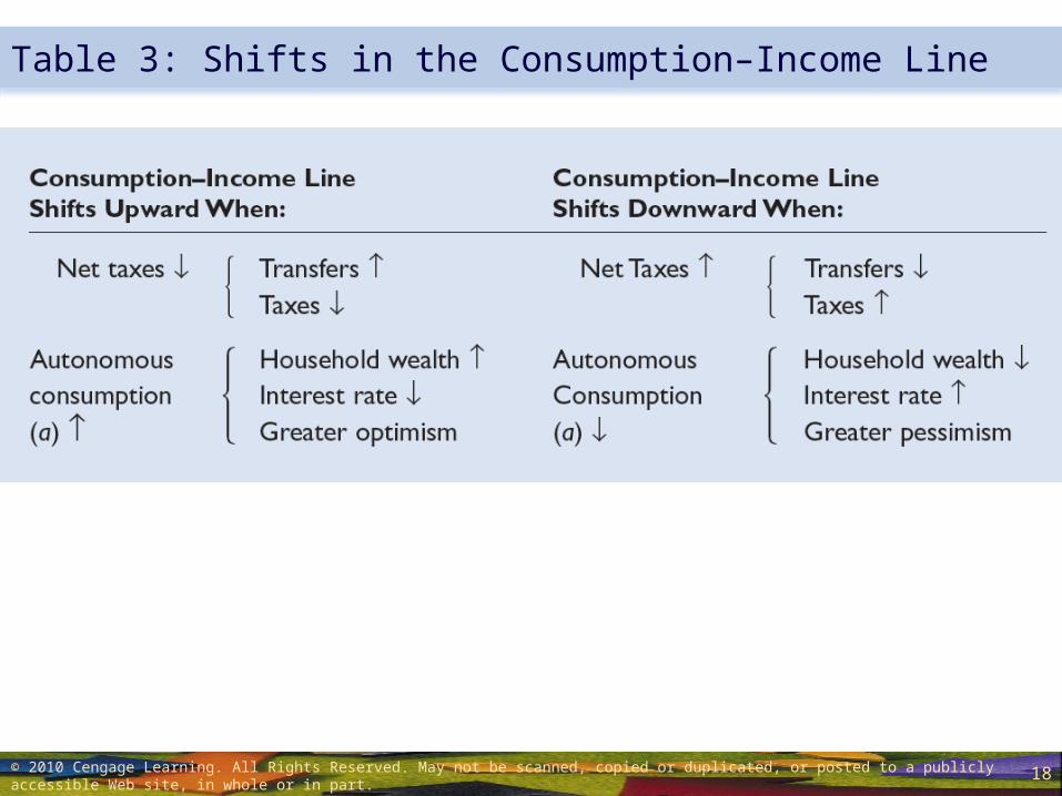
Table 3: Shifts in the Consumption–Income Line
© 2010 Cengage Learning. All Rights Reserved. May not be scanned, copied or duplicated, or posted to a publicly accessible Web site, in whole or in part.
Page 19
19
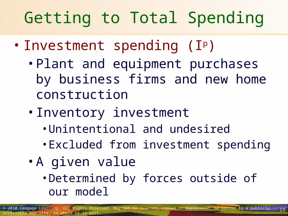
Getting to Total Spending
• Investment spending (Ip) • Plant and equipment purchases by business
firms and new home construction• Inventory investment
• Unintentional and undesired• Excluded from investment spending
• A given value• Determined by forces outside of our model
© 2010 Cengage Learning. All Rights Reserved. May not be scanned, copied or duplicated, or posted to a publicly accessible Web site, in whole or in part.
Page 20
20
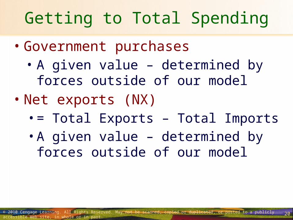
Getting to Total Spending
• Government purchases• A given value – determined by forces outside
of our model• Net exports (NX)
• = Total Exports – Total Imports• A given value – determined by forces outside
of our model
© 2010 Cengage Learning. All Rights Reserved. May not be scanned, copied or duplicated, or posted to a publicly accessible Web site, in whole or in part.
Page 21
21
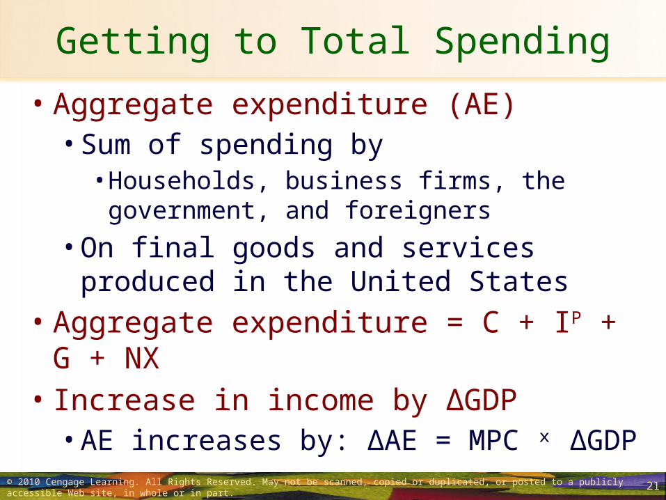
Getting to Total Spending
• Aggregate expenditure (AE)• Sum of spending by
• Households, business firms, the government, and foreigners
• On final goods and services produced in the United States
• Aggregate expenditure = C + IP + G + NX• Increase in income by ΔGDP
• AE increases by: ΔAE = MPC ˣ ΔGDP
© 2010 Cengage Learning. All Rights Reserved. May not be scanned, copied or duplicated, or posted to a publicly accessible Web site, in whole or in part.
Page 22
22
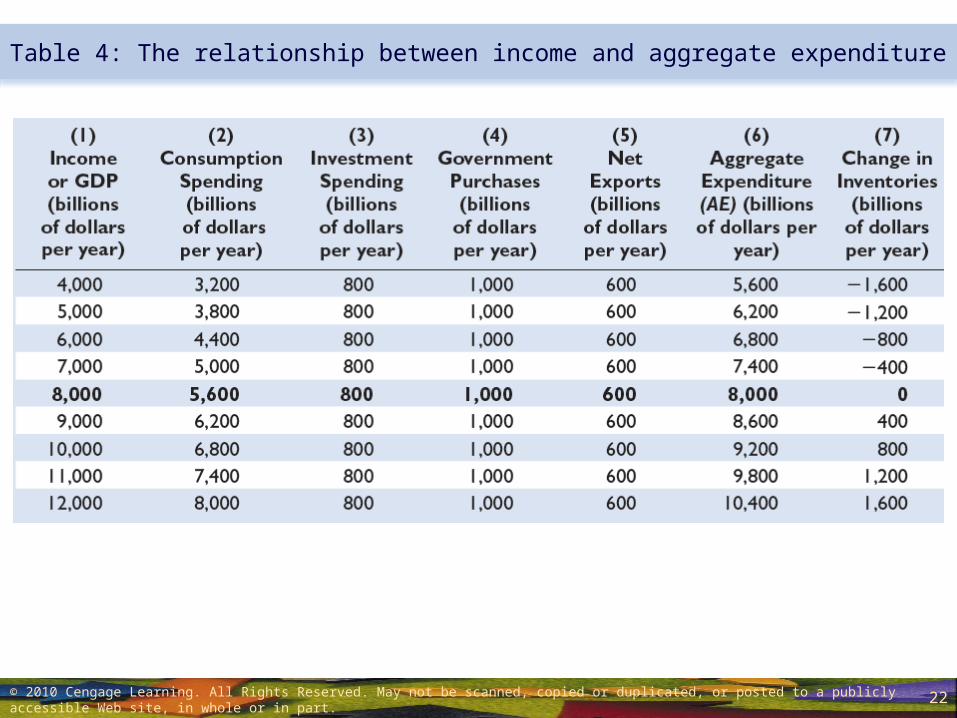
Table 4: The relationship between income and aggregate expenditure
© 2010 Cengage Learning. All Rights Reserved. May not be scanned, copied or duplicated, or posted to a publicly accessible Web site, in whole or in part.
Page 23
23
Equilibrium GDP
• When aggregate expenditure < GDP• Output will decline in the future
• When aggregate expenditure > GDP• Output will rise in the future
• Equilibrium GDP • In the short run• The level of output at which output and
aggregate expenditure are equal
© 2010 Cengage Learning. All Rights Reserved. May not be scanned, copied or duplicated, or posted to a publicly accessible Web site, in whole or in part.
Page 24
24
Equilibrium GDP
• Change in inventories • During any period • Will always equal output minus aggregate
expenditureΔ Inventories = GDP – AE
© 2010 Cengage Learning. All Rights Reserved. May not be scanned, copied or duplicated, or posted to a publicly accessible Web site, in whole or in part.
Page 25
25
Equilibrium GDP
• AE line• C, consumption-income line• C+IP at each level of income• C+IP+G at each level of income• AE line: C+IP+G+NX at each level of income• Slope = MPC
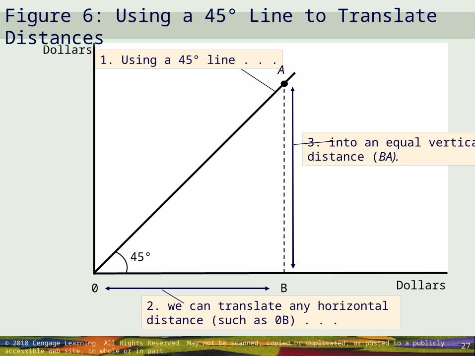
• A 45° line = translator line• It allows us to measure any horizontal
distance as a vertical distance instead
© 2010 Cengage Learning. All Rights Reserved. May not be scanned, copied or duplicated, or posted to a publicly accessible Web site, in whole or in part.
Page 26
26
Figure 5: Deriving the Aggregate Expenditure Line
© 2010 Cengage Learning. All Rights Reserved. May not be scanned, copied or duplicated, or posted to a publicly accessible Web site, in whole or in part.
Real GDP ($ billions)
ConsumptionFunction
Real AggregateExpenditure ($ billions)
2,000 4,000 6,000 8,000 10,000 12,000
12,000
10,000
8,000
6,000
4,000
2,000
1. Start with theconsumption–income line,
5. to get the aggregateexpenditure line.
CC + IP
2. then add planned investment (Ip) . . .
C + IP + G
3. government purchases (G) . . .
C + IP + G + NX
4. and net exports (NX) . . .
Page 27
27
Dollars
ConsumptionFunction
Dollars
0
Figure 6: Using a 45° Line to Translate Distances
© 2010 Cengage Learning. All Rights Reserved. May not be scanned, copied or duplicated, or posted to a publicly accessible Web site, in whole or in part.
1. Using a 45° line . . .
45°
B
A
2. we can translate any horizontal distance (such as 0B) . . .
3. into an equal verticaldistance (BA).
Page 28
28
Equilibrium GDP
• AE line below 45° line• AE < GDP• Inventories will grow• Reduce output in the future
• AE line above 45° line• AE > GDP• Inventories will decline• Increase their output in the future
© 2010 Cengage Learning. All Rights Reserved. May not be scanned, copied or duplicated, or posted to a publicly accessible Web site, in whole or in part.
Page 29
29
Figure 7: Determining Equilibrium Real GDP
© 2010 Cengage Learning. All Rights Reserved. May not be scanned, copied or duplicated, or posted to a publicly accessible Web site, in whole or in part.
Real GDP ($ billions)
ConsumptionFunction
Real AE ($ billions)
2,000 4,000 6,000 8,000 10,000 12,000
12,000
10,000
8,000
6,000
4,000
2,000
C+IP+G+NX
45°
A
HE
K
J
At point E, where the aggregate expenditure line crosses the 45° line, the economy is in short-run equilibrium. With real GDP equal to $8,000 billion, aggregate expenditure equals real GDP. At higher levels of real GDP—such as $12,000 billion—total production exceeds aggregate expenditures, and firms will be unable to sell all they produce. Unplanned inventory increases equal to HA will lead them to reduce production. At lower levels of real GDP—such as $4,000 billion—aggregate expenditure exceeds total production. Firms find their inventories falling, and they will respond by increasing production.
AggregateExpenditure
AggregateExpenditure
TotalOutput
TotalOutput
Decrease in inventories
Increase in inventories
Page 30
30
Equilibrium GDP
• Equilibrium GDP • AE line intersects the 45° line• No change in inventories• No change in output in the future
© 2010 Cengage Learning. All Rights Reserved. May not be scanned, copied or duplicated, or posted to a publicly accessible Web site, in whole or in part.
Page 31
31
Equilibrium GDP
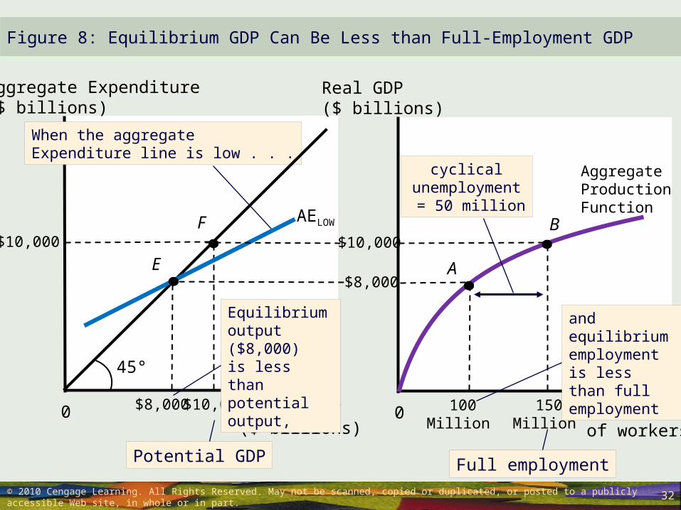
• Short-run equilibrium• And yet have abnormally high unemployment• Aggregate expenditure line is too low to
create an intersection at full-employment output
• Cyclical unemployment is caused by insufficient spending
• As long as spending remains low• Production will remain low• Unemployment will remain high
© 2010 Cengage Learning. All Rights Reserved. May not be scanned, copied or duplicated, or posted to a publicly accessible Web site, in whole or in part.
Page 32
32
Figure 8: Equilibrium GDP Can Be Less than Full-Employment GDP
© 2010 Cengage Learning. All Rights Reserved. May not be scanned, copied or duplicated, or posted to a publicly accessible Web site, in whole or in part.
Real GDP($ billions)
ConsumptionFunction
Aggregate Expenditure($ billions)
0
When the aggregateExpenditure line is low . . .
45°
$10,000
F $10,000
Potential GDP
AELOW
E
Equilibrium output ($8,000)is less than potential output,
$8,000 Number of workers
ConsumptionFunction
Real GDP($ billions)
0 150Million
$10,000
Full employment
and equilibrium employmentis less than full employment
100Million
$8,000
AggregateProductionFunction
A
B
cyclicalunemployment
= 50 million
Page 33
33
Equilibrium GDP
• Short-run equilibrium• And abnormally high employment and
abnormally low unemployment• Economy can overheat because spending is
too high• As long as spending remains high
• Production will exceed potential output• Unemployment will be unusually low
© 2010 Cengage Learning. All Rights Reserved. May not be scanned, copied or duplicated, or posted to a publicly accessible Web site, in whole or in part.
Page 34
34
Figure 9: Equilibrium GDP Can Be Greater than Full-Employment GDP
© 2010 Cengage Learning. All Rights Reserved. May not be scanned, copied or duplicated, or posted to a publicly accessible Web site, in whole or in part.
Real GDP($ billions)
ConsumptionFunction
Aggregate Expenditure($ billions)
0
When the aggregateExpenditure line is high . . .
45°
$10,000
F $10,000
Potential GDP
AEHIGHE’
Equilibrium output ($12,000)is greater than potential output,
$12,000
Number of workers
ConsumptionFunction
Real GDP($ billions)
0 150Million
$10,000
Full employment
and equilibrium employmentis greater than full employment
200Million
$12,000
AggregateProductionFunction
HB
Page 35
35
What Happens When Things Change?
• Increases in investment by $x• $x additional sales revenue• $x additional income• $x additional disposable income• MPC ˣ $x additional consumption spending• MPC ˣ $x additional sales revenue• …• …• Equilibrium GDP rises by a multiple of $x
© 2010 Cengage Learning. All Rights Reserved. May not be scanned, copied or duplicated, or posted to a publicly accessible Web site, in whole or in part.
Page 36
36
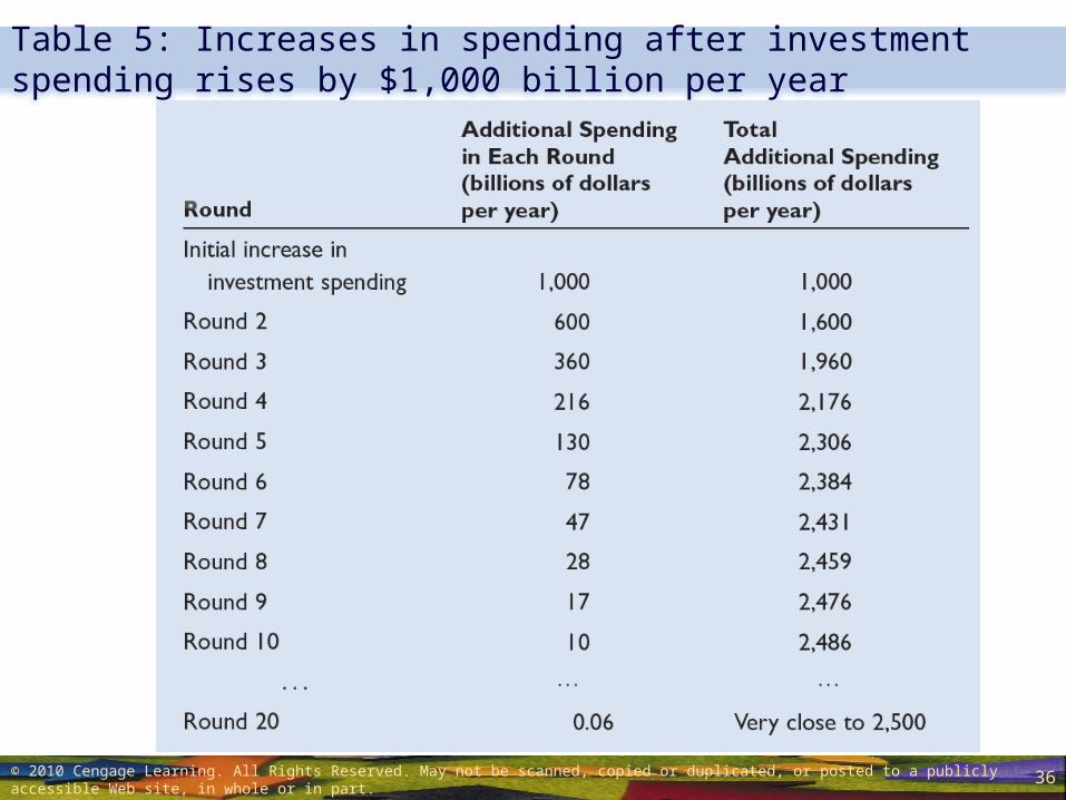
Table 5: Increases in spending after investment spending rises by $1,000 billion per year
© 2010 Cengage Learning. All Rights Reserved. May not be scanned, copied or duplicated, or posted to a publicly accessible Web site, in whole or in part.
Page 37
37
Figure 10: The Effect of a Change in Investment Spending
© 2010 Cengage Learning. All Rights Reserved. May not be scanned, copied or duplicated, or posted to a publicly accessible Web site, in whole or in part.
An increase in investment spending sets off a chain reaction, leading to successive rounds of increased spending and income. As shown here, a $1,000 billion increase in investment spending first causes real GDP to increase by $1,000 billion. Then, with higher incomes, households increase consumption spending by the MPC times the change in disposable income.
In round 2, spending and GDP increase by another $600 billion. In succeeding rounds, increases in income lead to further changes in spending, but in each round the increases in income and spending are smaller than in the preceding round.
Page 38
38
What Happens When Things Change?
• ΔGDP = Expenditure multiplier ˣ ΔIP • Expenditure multiplier
• The amount by which equilibrium real GDP changes
• As a result of a one-dollar change in:• Autonomous consumption, • Investment spending, • Government purchases, • Or net exports
© 2010 Cengage Learning. All Rights Reserved. May not be scanned, copied or duplicated, or posted to a publicly accessible Web site, in whole or in part.
Page 39
39
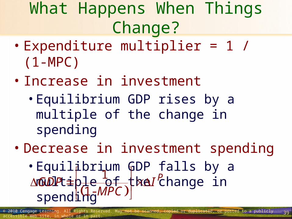
What Happens When Things Change?
• Expenditure multiplier = 1 / (1-MPC)• Increase in investment
• Equilibrium GDP rises by a multiple of the change in spending
• Decrease in investment spending • Equilibrium GDP falls by a multiple of the
change in spending
© 2010 Cengage Learning. All Rights Reserved. May not be scanned, copied or duplicated, or posted to a publicly accessible Web site, in whole or in part.
1
1-PGDP I
MPC
Page 40
40
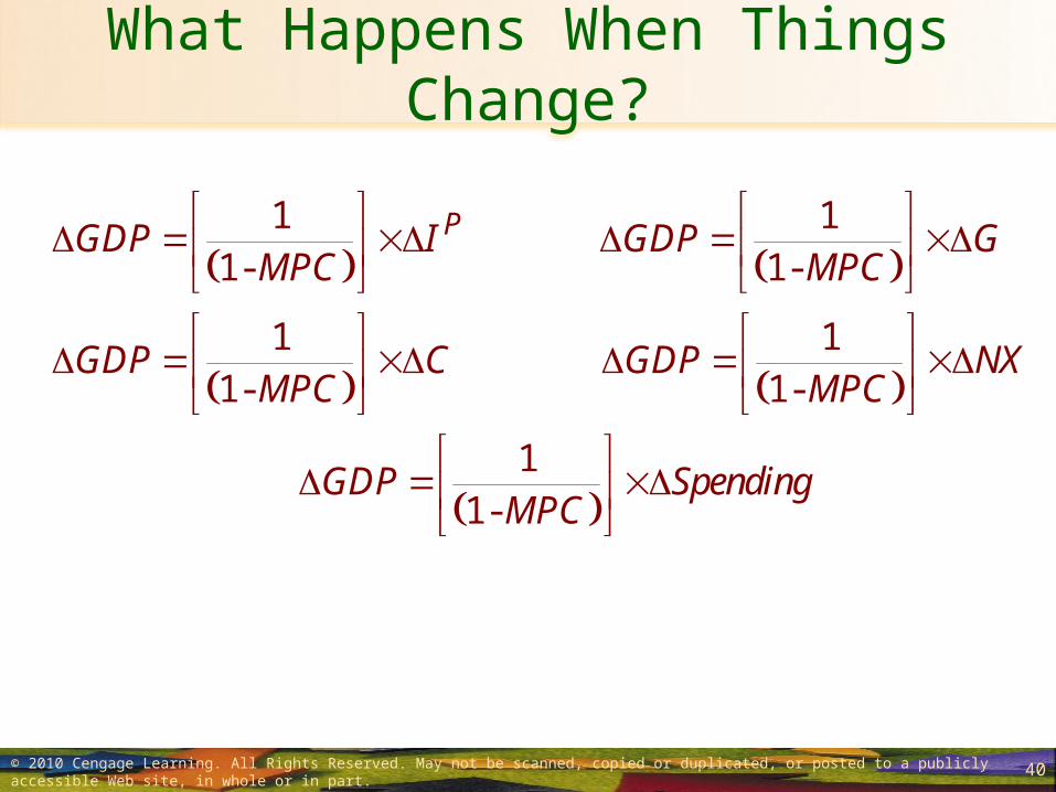
What Happens When Things Change?
© 2010 Cengage Learning. All Rights Reserved. May not be scanned, copied or duplicated, or posted to a publicly accessible Web site, in whole or in part.
1 11- 1-
1 11- 1-
11-
PGDP I GDP GMPC MPC
GDP C GDP NXMPC MPC
GDP SpendingMPC
Page 41
41
Figure 11: A Graphical View of the Multiplier
© 2010 Cengage Learning. All Rights Reserved. May not be scanned, copied or duplicated, or posted to a publicly accessible Web site, in whole or in part.
Real GDP ($ billions)
ConsumptionFunction
Real AE ($ billions)
2,000 4,000 6,000 8,000 10,000 12,000
12,000
10,000
8,000
6,000
4,000
2,000
AE1
45°
E
The economy starts off at point E with equilibrium real GDP of $8,000 billion. A $1,000 billion increase in spending shifts the aggregate expenditure line upward by $1,000 billion, triggering the multiplier process. Eventually, the economy will reach a new equilibrium at point F, where the new, higher aggregate expenditure line crosses the 45° line. At F, real GDP is $10,500 billion, an increase of $2,500 billion.
AE2
F
$1,000Increase inEquilibrium GDP = $ 2,500 Billion
Page 42
42
What Happens When Things Change?
• An increase in:• Autonomous consumption spending,
investment spending, government purchases, or net exports
• Will shift the aggregate expenditure line upward • By the initial increase in spending
• Equilibrium GDP will rise • By the initial increase in spending times the
expenditure multiplier
© 2010 Cengage Learning. All Rights Reserved. May not be scanned, copied or duplicated, or posted to a publicly accessible Web site, in whole or in part.
Page 43
43
The Multiplier Process and Economic Stability
• The larger the multiplier• The more unstable the economy • All else equal
• Automatic stabilizer • Feature of the economy • Reduces the size of the expenditure multiplier • Diminishes the impact of spending changes on
real GDP• Reduce fluctuations in GDP and employment• Makes the economy more stable in the short run
© 2010 Cengage Learning. All Rights Reserved. May not be scanned, copied or duplicated, or posted to a publicly accessible Web site, in whole or in part.
Page 44
44
The Multiplier Process and Economic Stability
• Taxes and transfers depend on income• Increase in income
• Higher taxes• Lower transfers • Less spending each round• Smaller multiplier
© 2010 Cengage Learning. All Rights Reserved. May not be scanned, copied or duplicated, or posted to a publicly accessible Web site, in whole or in part.
Page 45
45
The Multiplier Process and Economic Stability
• Imports depend on income• Increase in income
• Increase spending on imports• Smaller spending on domestic output
• Each round
• People - economic fluctuations as temporary• Spending - less sensitive to changes in income• Smaller spending changes
• Each round
© 2010 Cengage Learning. All Rights Reserved. May not be scanned, copied or duplicated, or posted to a publicly accessible Web site, in whole or in part.
Page 46
46
The Multiplier Process and Economic Stability
• Automatic de-stabilizers• Feature of the economy• Increases the size of the expenditure
multiplier • And enlarges the impact of spending changes
on real GDP• Enlarge fluctuations in GDP and employment• Makes the economy less stable in the short run
© 2010 Cengage Learning. All Rights Reserved. May not be scanned, copied or duplicated, or posted to a publicly accessible Web site, in whole or in part.
Page 47
47
The Multiplier Process and Economic Stability
• Household wealth • Changes with income• Rising income
• Rising wealth• Rising consumption spending• Larger multiplier effect on GDP
© 2010 Cengage Learning. All Rights Reserved. May not be scanned, copied or duplicated, or posted to a publicly accessible Web site, in whole or in part.
Page 48
48
The Multiplier Process and Economic Stability
• Investment spending• Changes during the multiplier process• GDP rises
• Increase investment• Larger multiplier effect on GDP
© 2010 Cengage Learning. All Rights Reserved. May not be scanned, copied or duplicated, or posted to a publicly accessible Web site, in whole or in part.
Page 49
49
The Multiplier Process and Economic Stability
• In the long run• Given the growth of potential GDP• The value of the expenditure multiplier is zero
• No matter what the change in spending• Economy will ultimately return to its potential
GDP—just as it would have without the spending change
© 2010 Cengage Learning. All Rights Reserved. May not be scanned, copied or duplicated, or posted to a publicly accessible Web site, in whole or in part.
Page 50
50
The recession of 2008–2009• Recession in U.S., causes
1. 2007, spike in oil prices• Decrease spending in automobiles• Laid-off workers
2. 2007, collapse of the housing bubble• Rapid fall in home prices
• Decline in wealth• Decline in autonomous consumption spending• AE line shifted downward
• Investment spending fell• AE line shifted downward
© 2010 Cengage Learning. All Rights Reserved. May not be scanned, copied or duplicated, or posted to a publicly accessible Web site, in whole or in part.
Page 51
51
The recession of 2008–2009• Recession in U.S., causes:
3. 2008, financial crisis• Defaults on mortgage payments• Decrease in lending throughout the economy• Fear and gloom about the economy’s future
• Households - cut back dramatically on spending
• Corporate profits - falling• Share prices - began to plummet• Major hit to household wealth
© 2010 Cengage Learning. All Rights Reserved. May not be scanned, copied or duplicated, or posted to a publicly accessible Web site, in whole or in part.
Page 52
52
The recession of 2008–2009• Automatic de-stabilizers:
• Falling output caused falling asset prices• Homes and stocks
• Falling asset prices led to further decreases in spending and output
• By the end of the process• Wealth of U.S. households declined by $14
trillion in a little over a year
© 2010 Cengage Learning. All Rights Reserved. May not be scanned, copied or duplicated, or posted to a publicly accessible Web site, in whole or in part.
Page 53
53
Figure 12a: Consumption and investment 2006-2009
© 2010 Cengage Learning. All Rights Reserved. May not be scanned, copied or duplicated, or posted to a publicly accessible Web site, in whole or in part.
Page 54
54
Figure 12b: Consumption and investment 2006-2009
© 2010 Cengage Learning. All Rights Reserved. May not be scanned, copied or duplicated, or posted to a publicly accessible Web site, in whole or in part.
Page 55
55
The recession of 2008–2009• Automatic stabilizers:
• Government’s tax revenues fell and transfer payments rose• Helping to cushion the decline in disposable
income and maintain spending• Imports declined
• Shifting some of the impact of lower spending to firms in other countries
© 2010 Cengage Learning. All Rights Reserved. May not be scanned, copied or duplicated, or posted to a publicly accessible Web site, in whole or in part.
Page 56
56
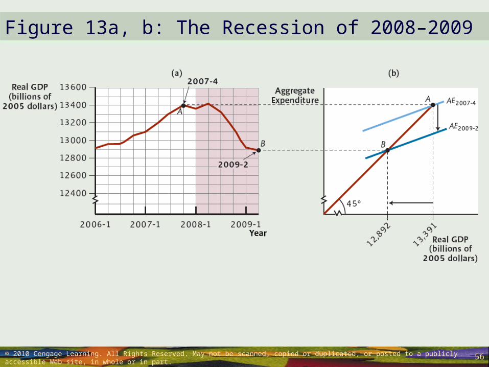
Figure 13a, b: The Recession of 2008–2009
© 2010 Cengage Learning. All Rights Reserved. May not be scanned, copied or duplicated, or posted to a publicly accessible Web site, in whole or in part.
Page 57
57
Figure 13c: The Recession of 2008–2009
© 2010 Cengage Learning. All Rights Reserved. May not be scanned, copied or duplicated, or posted to a publicly accessible Web site, in whole or in part.
Page 58
58
The recession of 2008–2009• Recession in other countries
• Global recession, closely synchronized• Other countries – housing boom and bust
• At the same time• Lengthy period of low interest rates around the
globe• Leverage and speculation
• Financial crisis
© 2010 Cengage Learning. All Rights Reserved. May not be scanned, copied or duplicated, or posted to a publicly accessible Web site, in whole or in part.
Page 59
59
The recession of 2008–2009• Recession in other countries
• Germany and Japan • Did not have housing bubbles
• Very strong growth in exports• Especially severe downturns
• Because of net exports
© 2010 Cengage Learning. All Rights Reserved. May not be scanned, copied or duplicated, or posted to a publicly accessible Web site, in whole or in part.
Page 60
60
Figure 14: The Recession of 2008–2009 in Selected Countries
© 2010 Cengage Learning. All Rights Reserved. May not be scanned, copied or duplicated, or posted to a publicly accessible Web site, in whole or in part.


![a n 1nurul_a.staff.gunadarma.ac.id/Downloads/files/59525/... · Membuat Aplikasi Macro •Jalankan macro dengan pilih menu Run > Run Sub/UserForm ata u tekan tombol [F5], macro tersebut](https://static.documents.pub/doc/80x56/60bd23ce0ad60057663be617/a-n-1nurulastaff-membuat-aplikasi-macro-ajalankan-macro-dengan-pilih-menu-run.jpg)


