SHORT-TERM ANALYSIS OF

MACROECONOMIC TIME SERIES

Agustin Maravall

Banco de España - Servicio de EstudiosDocumento de Trabajo nº 9607

SHORT-TERM ANALYSIS OF

MACROECONOMIC TIME SERIES

Agustin Maravall

Banco de Espana - Servicio de Estudios Documento de Trabajo n' 9607

In publishing this series the Banco de Espana seeks to disseminate studies of interest that will help acquaint readers better

with the Spanish economy:

The analyses, opinions and findings of these papers represent the views of their authors: they are Dot necessarily those

of the Banco de Espana.

ISSN: 0213-2710

ISBN: 84-7793-462-2

Dep6sito legal: M·9882·1996

Imprenta del Banco de Espana

Abstract

The paper deals with the statistical treatment of macroeconomic data for short-run economic analysis, monitoring and control. The main applications are short-term forecasting and unobserved components estimation, including trend and cycle estimation, and, most often, seasonal adjustment. The paper briefly reviews some of the recent developments in the field, both at the methodolOgical and applied levels. Then, it is argued that a fairly general. approach, based on signal extraction methods and ARlMA models, will gradually spread as the dominant methodology. The last section contains a word of caution, and illustrates the danger of applying these short-term statistical tools to long-term economic analysis.

-3-

1 Introduction

I shall be talking about statistical treatment of short-term macroecon�mic data. In particular, I shall focuss on monthly time series of standard macroeconomic aggre­gates, such as monetary aggregates, consumer price indices, industrial production indices, export and import series, employment series, to quote a few examples.- The statistical treatment considered is that aimed at helping economic policy makers in short-term control, and at facilitating monitoring and interpretation of the economy by analysists in general. The purpose of the statistical treatment is to answer two basic questions, well summarized by P.G. Wodehouse when answering a question concerning his physical shape (Wodehouse, 1981, p. 577): "The day ·before yester­day, for instance, (the weighing machine in my bathroom) informed me -' and I don't mind telling you, J.P., that it gave me something of a shock - tha� I weighed seventeen stone nine. I went without lunch and dined on a small biscuit and a stick of celery, and next day I was down to eleven stone one. This was most satisfactory and I was very pleased about it, but this morning I was up again to nineteen stone six,· so I really don't know where I am or what the future holds." The two separate - though related - questions are:

(a) where are we? (b) where are we heading?

Of course, forecasting provides the answer to (b). The answer to question (a) usually consists of an estimation of the present situation, free of seasonal variatioDj on occasion, variation judged transitory is also removed. Thus seasonal adjustment and trend estimation are used to answer question (a). For monthly macroeconomic series, it is often the case that seasonal variation dominates the short-run variability of the series.

In the next sections I will briefly review the recent evolution of the statistical methodology used in this context, and will provide a Uustified) forecast of how I would expect it to evolve over the next ten years. The discussion will address the evolution in terms of research and in terms of practical applications (such as, for example, official seasonal adjustment). While the former typically contains a lot of noise, practical applications lag research by several (sometimes many) years.

W henever confronted with forecasting an event, one is bound to look first at the present and past history. I shall do that, and from the (critical) look, my forecast will emerge in a. straightforward and unexciting manner. The discussion centers on tools used for short-term analysis; at the end we present an example that illustrates the unreliability of these tools when our horizon is a long-term one.

2 Short-Term Forecasting

I shall start with a very brief mention to short-term forecasting in economics. Leav­ing aside judgemental (or "expert") forecasting, in the remote past, some determin-

-5-

istic models, such as for example models with linear trends and seasonal dummies

were used for short-term forecasting. This practice gave way to the use of "ad hoc" filters, which became popular in the fifties and sixtiesj examples are the exponen­tially weighted moving average method (Winters, 1960), and the discounted least squares method of Brown (1962). In the decade of the seventies, the work of Box

and Jenklns (1970) .provoked a revolution in the field of applied forecasting; this revolution was further enhanced by another factor: the discovery by economic fore­casters of the Kalman Filter (see, for example, Harrison and Stevens, 1976). The Box-Jenkins approach offered a powerful, easy to learn and easy to apply, method­ology for short-term forecastingj the Kalman filter provided a rather convenient tool to apply and extend the methodology.

The outcome was a massive spread. of statistical models (simple parametric stochastic processes) and, in particular, of the so-called Autoregressive Integrated Moving Average (ARIMA) model, and of its several extensions, such as Intervention Analysis and Transfer Function models (see Box and Tiao, 1975, and Box and

Jenklns, 1970), and of the closely related Structural Time Series models (see Harvey, 1989). One can safely say that ARIMA models are used everyday by thousands of practitioners. Some use is also made of multivariate versions of these models (for example, see Litterman, 1986), although multivariate extensions have often been frustrating. A good review of the economic applications of time series models is contained, for example, in Mills (1990).

The point we wish to make for now is that, overall, stochastic model-based forecasting has become a standard procedure. At present, two important directions of research are:

(1) Multivariate extensions, where the relatively recent research on cointegration and common factors may lead to an important break (through a reduction in dimensionality and an improved model specification).

(2) Nonlinear extensions, such as the use of bilinear, ARCH, GARCH, stochastic

parameter models, and 50 on.

I would expect direction (1) to eventually play a very important role in applied short-term forecasting over the next decade. As for the future impact of direction (2), I doubt that in the next years stochastic nonlinear models will become a stan­dard tool for the average practitioner.

3 Unobserved Components Estimation and Sea­

sonal Adjustment

Back to question (a) of section I, we proceed. to the problem of estimating the rele­vant underlying evolution of an economic variable, that is, to seasonal adjustmentj we shall also consider some trend estimation issues. Two good references that de­scribe the present state of the art concerning seasonal adjustment are Den Butter

-6-

and Fase (1991) and Hylleberg (1992). As with forecasting, deterministic models were used in the distant past. At present, however, I do not know of any official agency producing monthly seasonally adjusted macroeconomic data that removes seasonality with deterministic dummy variables. (In fact, the only major use of deterministic seasonal adjustment at present seems to be academic research!) \

It is widely accepted by practitioners that, typically, seasonality in macroeco­nomic series is of the moving type, for which the use of filters is appropriate. H Xt denotes the series of interest (perhaps in logs), nt the seasonally adjusted series, and St the seasonal component, a standard pr6cedui'e is to assume

and to estimate St by 5, = G{B) x" (I)

where B is the lag operator such that B' x, = x,_. (k integer), and G{B) is the linear and symmetric filter

G{B) = "" + c1{B + F) + ... + c,.{B' + F), (2)

with F = B-1. Of course, the filter G{B) is designed to capture variability of the series in a (small) interval around each seasonal frequency. The seasonally arljusted series is, in turn, estimated by

n, = [1 - G{B)] x, = A{B) x" (3)

and A(B) is also a centered, linear, and symmetric filter. The symmetric and complete filters (I) and (3) cannot be uaed to estimate ;,

or � when t is close to either end of the series. Specifically, at time T, when the available series is (Xl, .. " XT)' estimation of St with (1) for t < T requ,ires unavail­able starting values of Xj analogously, estimation of St for t > T - r requires future observations not yet available. Therefore, the centered and symtnetric filter charac­terizes "historical" estimates. For recent enough periods asymmetric filters have 'to be used, which yield preliminary estimators. As time passes and new observations become available, those preliminary estimators will be revised until the historical at­

final estimator is eventually obtained. To this issue we shall come back later. In the same way tha.t 1970 marks an important date for applied sho�-term

forecasting (Le., the year of publication of the book by Box and Jenkins), 1967 marks a crucial event in the area of seasonal adjustment. That event was the appearance of the program XU, developed by the U.S. Bureau of the Census (see Shiskin et al" 1967). Except for some outlier treatment (which we shall ignore), XU can be seen as a sequence of linear filters, and hence as a linear filter itself (see, for example, Hylleberg, 1986). For the discussion that follows, we use the parsinionious approximation to XU (historical filter) of Burridge and Wallis (1984). Figure 1 plots the transfer function (in the frequency domain) ofthe XU monthly filter A{B). This

-7-

transfer function represents, for each frequency, which proportion of the variablity of Xt is used to estimate the seasonally adjusted series. It is seen how the XU filter passes the variation associated with all frequencies, except for some small intervals around the seasonal ones.

Over the next decade, XU spread at an amazing speed, and many thousands of series came to be routinely adjus�ed with XII. It was an efficient and easy-to­use procedure that seemed to provide good results for many series (although the meaning of "good" for seasonal adjustment is somewhat unclear). Yet, towards the end of the seventies some awareness of Xll limitations started to develop. Those limitations were mostly associated with the rigidity of the Xll filter, i.e., with its "ad hoc" relatively fixed structure. To these limitations we turn next.

4 Limitations of Ad-hoc Filtering

We shall provide simple illustrations of some major limitations of fixed ad-hoc filters such as XU.

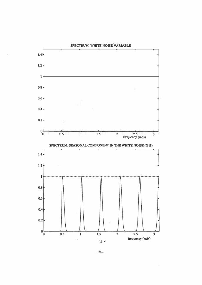
(1) The danger �f spurious adjustment is illustrated in figure 2. In a white-noise series, with spectrum that of part a in the figure, XU will extraet a seasonal component, with spectrum that of part b. This spectrum is certaintly that of a seasonal component, but the series had no seasonality to start with.

(2) In the previous white-noise series, trivially, the filter A(B) to seasonally adjust the series should simply be 1 i on the other extreme; if the observed series has a spectrum as in part b of figure 2, the filter to seasonally adjust the series should obviously be 0, since the series only contains seasonal variation. The filter should depend, thus, on the characteristics of the series.

To illustrate the point, we use the well-known "Airline model" of Box and Jenkins (1970, chap. 9). It is a model appropriate for monthly series displaying trend and seasonality. For series in logs, the model implies that the annual difference of the monthly rate of growth is a stationary process. The Airline model is, on the one hand, a model often encountered in practice; on the other hand, it provides an excellent reference example. The model is given by the equation

(4)

where jJ is a constant, at; is a white-noise innovation (with variance Va), V = 1 - B, V12 = 1 - B12, and -1 < 81 < 1, ° < 812 < 1. The series Xt. generated by (4), accepts a rather sensible decomposition into trend, seasonal, and irregular component (see Hillmer and Tiao, 1982). As 01 approaches 1, model (4) tends towards the model

'V';, X, = (1- 01, Bl') a, + J1<J + ",t,

-8-

with deterministic trend. Similarly, when 812 becollH's 1. t.h(' S(�c\..",onal compo­

Hent becomes deterministic. Thus, t.he paraBl('h'!' HI(H1:.!) 11li��' be interpreted as a measure of how close t.o det.erministic tlip trend (:-:l'H-sOIml) component is.

In the frequency domain this '"clos('r to dl,tl'r1uillistil''' behavior of a compo­

nent is associated wit.h t.he width l)f tht' :,pl't'tral }leaks. Tlms, for example,

figure 3 displays the spectnl of two :'t'ril':' htlt h tl11lnwing models of the type (4).

The one wit.h the continuous lint' ('(Hit'lill:' llll1rt' st.ochastic: seasonal variation!

in a('('ordance wit.h tht' widt'r spl'l'tml pt'aks for t.he seasonal frequencies. The

seasonal component in th(' st'rit':' with spt'C'tnull given by the dotted line will be

more st.able. and ht'Ill't' cil1::,t'r to dt'terministic. Since the XU seasonal adjust­

ment. filter di::;phl�'S holt's of fi'Xed width for the seasonal frequencies, it follows

t.hat XU will tluderadjust when the width of the seasonal peak in the series

spect.rum is larger than that captured by the XU filter. Figure 4a illustrates

t.his situation. and Figure 4b displays the spectrum of the estimated season­

ally adjusted series obtained in this case. The underadjustment is reflected

in the two peaks that remain in the neighborhood of each seasonal frequency:

obviously XU has not removed all seasonal variation from the series. (This

type of underadjustment is often found when using XU on series of Industrial

Production Indices).

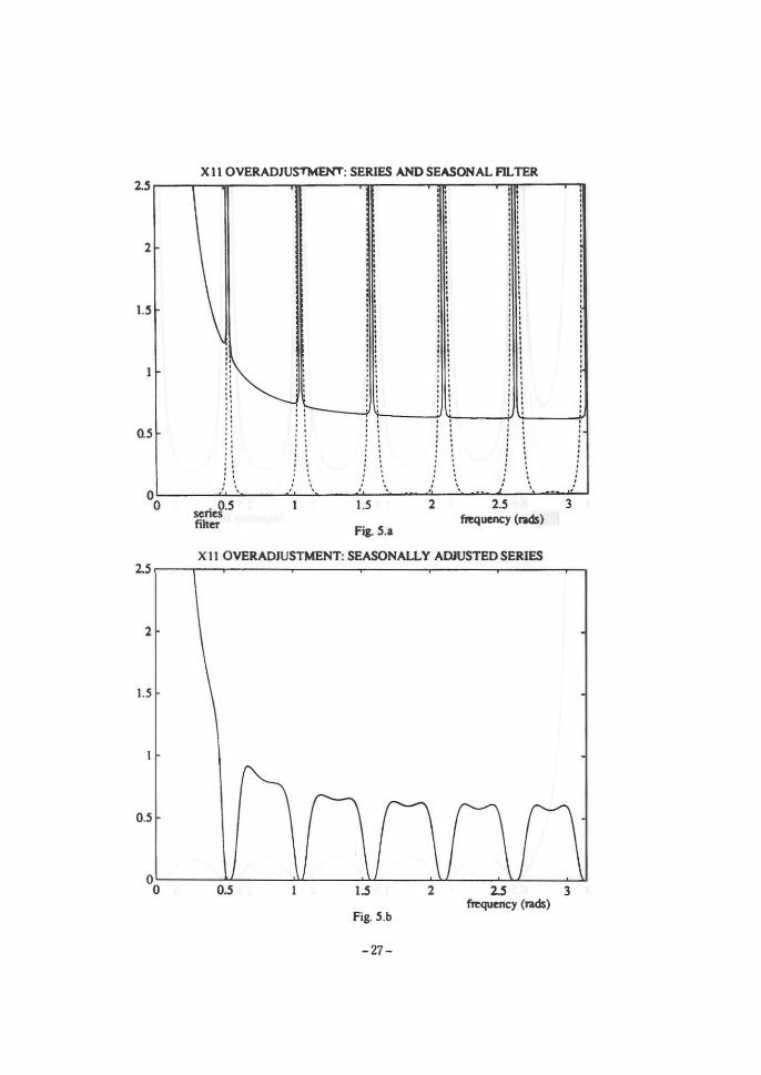
On the other hand, XU will overadjust (i.e.! will remove too much variation

from the series) when the width of the seasonal spectral peaks are narrower

than those captured by XII. This effect is evidenced in figure 5: the holes in

the seasonally adjusted series spectrum (part b of the figure) are now too wide. (This type of over adjustment is often found when applying XII to Consumer

Price Indices).

(3) Another limitation of XU is the lack of a proper framework for detecting the

cases in which its application is inappropriate. On the one hand! diagnostics are few and difficult to interpret. Moreover, when found inappropriate, there

is no systematic procedure to overcome the inadequacies.

(4) Even when appropriate, XU does not contain the basis for proper inference.

For example, what are the standard errors associated with the estimated sea­

sonal factors? This limitation has important policy implications (see Bach

et al., 1976, and Moore et al., 1981). In short-term monetary control, if the

monthly target for the rate of growth of Ml (seasonally adjusted) is 10% and

actual growth for that month turns out to be 13%, can we conclude that

growth has been excessive and raise, as a consequence, short-term interest

rates? Can the 3 percent points (p.p.) difference be attributed to the error

implied by the estimation of the seasonally adjusted series? Similarly, when

assessing the evolution of unemployment, if the series of total employment

grows by 90.000 persons in a quarter, and the seasonal effect for that quarter

is estimated as an increase of 50.000 persons, can we assume that the increase

has been more than a pure seasonal effect?

- 9-

(5) In the same way that XlI does not provide answers to these questions, it

does not allow us to compute optimal forecasts of the components. (Seasonal

factors for the year ahead are simply computed by adding to this year factors

one half of the difference between them and the factors one year before. Of

course, there is no measure of the uncertainty associated with these forecasts.)

(6) Although XlI computes separate estimates of the trend, seasonal, and irreg­

ular components, their statistical properties are not known. Therefore, it is

not possible to answer questions such as, for example, whether the trend or

the seasonally adjusted series provide a more adequate signal of the relevant

underlying evolution of the series (see Kenny and Durbin, 1982, Moore et al., 1981, and Marava.ll and Pierce, 1986).

To overcome some of those limitations, throughout the years Xll has been

subject to modifications. In particular, the program Xll ARIMA, developed by

Statistics Canada (see Dagum, 1980), improved upon XlI in several ways. First,

it incorporated several new elements for diagnosis. Perhaps more relevantly, it pro­

vided better estimators of the components at the end of the series. This was achieved

by replacing the ad-hoc XII filters for the preliminary estimators with a procedure

in which the series is extended with ARIMA forecasts, so that the filter A(B) can

be applied to the extended series (and hence to more recent periods). In fact, Xll ARIMA has replaced Xll in many standard applications.

At present, the U.S. Bureau of the Census is experimenting with a new program

for seasonal adjustment: X12 ARIMA (see Findley et al., 1992). The program follows

the direction of Xll ARIMA, and incorporates some new sets of diagnostics and

some new model-based features, having to do with the treatment of outliers and with estimation of special effects.

Be that as it may, practical applications (such as "official" seasonal adjustment

by agencies) lag with respect to research. So, let us turn to the evolution of (mostly

academiC) research during the last 10 or 15 years.

5 T he Model-Based Approach

Towards the end of the seventies and beginning of the eighties a new approach to the

problem of estimating unobserved components in time series, and in particular to

seasonal adjustment, was developed. The approach combined two elements: one, the

use of simple parametric time series models (mostly, of the ARIMA type); second, the

use of signal extraction techniques. Although there were earlier attempts at using

signal extraction on time series models (see Nerlove, Grether, and Carvalho, 1979), these attempts were of limited interest because they were restricted to stationary

series, while economic series are typically nonstationary.

The model-based approach has followed two general directions. One is the so­

called ARIMA-Model-Based methodology,.8J!.d some relevant references are Burman

� 10-

(1980). Hillmer and Tiao (1982). Bell and Hillmer (1984). and Maravall and Pierce

(1987). The second direction follows the so-<:alled Structural Time Series methodol­

ogy. and some important references are Engle (1978). Harvey and Todd (1983). and

Gersch and Kitagawa (1983). We shall refer to them as the AMB approach and the

STS approach, respectively. Both are closely related, and share the following basic

structure:

The observed series {xd = [Xl, ... ,xTl can be expressed as the sum of several

orthogonal components,

where each component Xit may be expressed as an ARIMA process (with Gaussian

innovations). Thus, for example, the model for the trend, Pt. may be of the type

where 6p(B) is a polynomial in B, and the model for the seasonal component, St. is

often of the form (for monthly series):

(I + B + ... + B") s, = B,{B) a,to

specifying that the sum of 12 consecutive seasonal components is a zero-mean sta­

tionary process (with "small" variance). While the trend and seasonal components are typically nonstationary, the irregular component is a zero-mean stationary pro­cess, often simply white-noise. Since the sum of ARIMA models yields an ARIMA model, the observed series Xt also follows an ARIMA model, say

<I>{B) x, = B{B) a,. (5)

where ¢(B) contains the stationary and nonstationary autoregressive roots.

Once the models are specified, the unobserved components are estimated as the Minimum Mean Squared Error (MMSE) estimator

x" = E{x" I [x,)). (6)

and this conditional expectation is computed with signal extraction techniques.

(This technique is a fairly general procedure that can be applied to a variety of statistical problems besides unobserved components estimation. In particular, fore­

casting can be seen as the particular case when Xit is the estimator of a future ob­

servation; another well-known application is interpolation of missing values.) The

MMSE estimator (6) obtained in the model-based approach is also a linear filter,

symmetric, centered, and convergent in both directions of the past and of the future.

Thus, as was the case with filter (2), the filter applies to historical estimates, and

the problem of preliminary estimation and revisions again reappears. The model­

based approach offers an optimal solution: the observed series are extended with

forecasts (and backcasts) as needed, and the symmetric and centered. filter can then

-11-

be applied to the extended series. (In terms of the observed values, the filter will be, of course, asymmetric; see Cleveland and Tiao, 1976.)

The decomposition of Xt into unobserved components presents a basic iden­

tification problem. In general, the AMB and STS methods use somewhat different

assumptions in order to reach identification; these different assumptions, of course,

lead to differences in the specification of the component models. It is the case, however, that the STS trend and seasonal components can be expressed as the ones obtained from an AMB approach with superimposed orthogonal white noise (see

Maravall, 1985). Ultimately, the crucial assumption for identification of the compo­

nents concerns the amount of variance assigned to the irregular; the AMB approach,

in order to maximize the stability of the trend and seasonal components, maximizes the irregular component variance.

Besides these differences in the specification of the component models, there

are some additional ones between the two approaches. The AMB method starts by specifying the model for the observed series, following standard Box-Jenkins techniques. From this aggregate model, the component models are then derived,

and the condition·al expectation (6) is obtained with the Wiener-Kolmogorov filter

(see Whittle, 1963, and Bell, 1984). On the contrary, the STS method starts by

directly specifying the models for the components, and uses the Kalman filter to

compute the conditional expectation (6); see Harvey (1989).

A simple example can illustrate the basic differences between the two model­

based approaches. Assume a non-seasonal series with possibly a unit root. The STS method would likely estimate the model

Xt = Pt + Ut, (7.a)

where Pt, the trend, follows the random walk model

(7.b)

and bt is white noise, orthogonal to the white-noise irregular Ut. The parameters that have to be estimated are two, namely the variances V(bt) and V(Ut).

That basic model implies that the observed series Xt follows an IMA(l,l) model,

say

Vx, = (1-BE)a,. (8)

A potential problem of the STS is that, since it does not include a prior identi­

fication stage, the model specified may be inappropriate. On the contrary, the AMB

approach first identifies the model with standard ARIMA-identification tools (there are indeed many available). If, in the AMB approach, the model identified. for the observed series turns out to be of the type (8), then the decomposition becomes:

- 12 -

(9.a)

(9.b)

and b; is white noise, orthogonal to the white-noise irregular u; . The factor (1 + B) in the MA part of (9.b) implies that the spectrum of p; is monotonically decreasing in the range (0,7r], with a zero at frequency 7r. It will be true that V(,,;) > V(",), and, in fact, Pt can be expressed as

where Ct is white noise, orthogonal to b;, and with variance [V(u;) - V(Ut)].

The example illustrates some additional differences. It is straightforward to find, for example, that model (7), the STS specification, implies the constraint 8 2: 0 (otherwise the irregular has negative spectrum). This constraint disappears in the AMB approach.

The parameters that have to be estimated in the STS approach are the vari­ance of the innovations in the components, V(Ut} and V(bt}; in the AMB approach, the parameters to estimate are those of a standard ARIMA model. Of course, the STS approach has a parsimonious representation in terms of the component's mod­els, and is likely to produce unparsimonious ARIMA expressions for the observed series. On the contrary, the AMB approach estimates a parsimonious ARIMA for the observed series, and the derived models for the components may well be unparsimo­nious. In both cases, estimation of the model is made by maximum likelihood. The component's estimators in the STS approach are obtained with the Kalman filter smoother, while in the AMB approach the Wiener-Kolmogorov filter is used. If the former filter offers more programming flexibility, the Wiener-Kolmogorov is more informative for analytical purposes.

Be that as it may, despite the differences, both methods share the same ba­sic structure of ARIMA components-ARIMA aggregate, where the components es­timators are the expectations conditional on the available observations (their least squares projections). Ultimately, both represent valid approaches. My (probably biased) view is that the AMB method, by using the data to identify the model, is less prone to misspecification. I find it reasonable, moreover, in the absence of additional information, to provide trend and seasonal components as smooth as possible, within the limits of the overall stochastic behavior of the observed series. FUrther, the AMB method typically implies direct estimation of fewer parameters, and provides results that are quite robust. a.nd numerically stable. On the other hand, the state space-Kalman filter format. in the STS m�thodology offers the ad­vantage of its programming and computational simplicity and flexibilit.y. In any case, both methods provide interesting a.nd relatively powerful t.ools for unobserved components estimation in linear stochastic processes. It is wort.h not.icing that many ad-hoc procedures can be given a minimum MSE-lIlOd(>I--h<l�('(i interpretation for part.icular ARIMA models (see, for example, Cleveland <l-nd TielO. 1976, Burridge and Wallis, 1984, and Maravall, 1993).

- 13-

6 The Virtues of a Model-Based Method

The major advantage of a model-based method is that it provides a convenient framework for straightforward statistical analysis. To illustrate the point we shall return to the 6 examples used when illustrating the limitations of ad-hoc filtering in section 4. As the model-based method, we use the AMB one and, in particular, a program called SEATS ("Signal Extradion in AruMA Time Series"); see Maravall and Gomez (1994). The program SEATS originally developed from a program built by Burman for seasonal adjustment at the Bank of England.

(1) The danger of spurious adjustment is certainly attenuated: if a series is white­noise, it would be detected at the identification stage, and no seasonal adjust­ment would be performed.

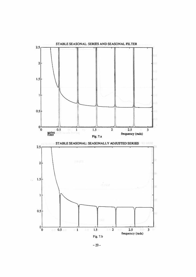
(2) The dangers of underadjustment (figure 4) and overadjustment (figure 5) are also greatly reduced. The parameters of the ARIMA model will adapt them­selves to the width of the spectra! peaks present in the series. Figure 6 illus­trates the seasonal adjustment (with the AMB method) of the series in figure 4: part (a) illustrates how the filter adapts itself to the seasonal spectral peaks, and part (b) shows how the spectrum ·of the estimated seasonally adjusted series shows no evidence now of underadjustment. AMB seasonal adjustment of the series with a very stable seasonal (the series of figure 5) is displayed in figure 7. The filter now captures a very narrow baDd, and the spectrum of the adjusted series estimator does not provide evidence of overadjustment.

(3) To illustrate how the model-based approarh can provide elements of diagnos­tics, we use an example from Maravall (1987). The example also illustrates how, when the dia�ostic is negative, one can proceed in order to improve upon the results.

When adjusting with XII the Spanish monthly series of insurance operations (a small component of the money supply), the program indicated that there was too much autocorrelation in the irregular estimator, Ut: In fact, the lag-l autocorrelation of Ut was .42. This seems large, but what would be the correct value for XII? There is no proper answer to this question.

For a model-based method with a white-noise irregular component, ut, the MMSE estimator Ut has the Autocorrelation Funcion (ACF) of the "inverse" model of (5), that is of the model obtained by interchanging the AR and the MA polynomials. Hence, given the model for the observed series, the theoretical value of the ACF for Ut is easily obtained. For the model-based interpretation of Xli (for which '" is white-noise), one finds PI (u.) � -.2 with a standard error of .1. Thus a 95% confidence interval for PI would be, approximately, (-.40, 0). Since the value obtained, .42, is far from the interval, in the model-based approach it is clear that there is indeed too much autocorrelation in the irregular.

-14-

The relative large, positive, autocorrelation in itt seems to indicatf} underesti­mation of the trend, which, to some degree, contaminates the irregular. The ARIMA model for which XU provides an MMSE filter contains the stationary transformation '\1 '\1 12. Having had a negative diagnostic, back to the identifi­cation stage, it was found that a model with the transformation '\12 '\112, which allowed for a more stochastic trend, provided a better fit of the series. For

'this

model, the theoretical value of PI (itt) was -.83, AMB decomposition of the series with the new model specification yielded an irregular with PI = -.82, with SE = .05., perfectly in agreement with what should have be�n obtained.

Thus the model-based approach offers a natural set-up for carrying out di­agnostics, and permits to improve upon the results by applying the standard iterations (identification/estimation/diagnosis, and back to identification) of a model-building procedure.

(4) As for the possibility of drawing inference, I mentioned the importance of measuring the errors associated. with the estimated components.

Given the model, the estimator (6) contains two types of errors. First, as mentioned in Section 3, when t is not far from the two ends of the series, a preliminary estimator will be obtained. Consider the case of concurrent estimation, that is the estimation of Xit when the last observation is Xt. As new observations become available, eventually the preliminary estimator will become the final one (i.e., the one that yields historical estimators). The difference between the preliminary and final estimator is the "revision err�r" . The second type of error is the one contained in the final estimator, implied by the" stochastic nature of the component. The revision error and the error in the final estimator are orthogonal (Pierce, 1980).

With the model-based. approach, it is straightforward to compute variances and autocorrelations of each type of error (see Maravall, 1994). Thus, in the examples used. in point (4) of section 4, the AMB method of SEATS yields the following answers: The standard error in the estimator of the monthly rate of growth of the seasonally adjusted Spanish monetary aggregate series is 1.95 percent points of annualized growth. Thus, with a 95% size we cannot reject the hypothesis that the measurement of 13% growth is in agreement with the 10% target. (If the size is reduced to 70%, then the measured growth becomes signlficantly different from the target.)

As for the quarterly series of Spanish employment, the standard error of the seasonal component estimator is equal to 19.000 pers<?ns. Thus the 90.000 increase could be (barely) accepted "" significantly more than the se""onal effect of 50.000.

.

(5) The model-based approach provides MMSE forecasts of the components, as well as their associated. standard errors. For example, for the Spanish monthly series of imports, the standard errors of the 1 and 12 periods-ahead forecasts

-15-

for the original series, the seasonally adjusted series, and the trend, are the

following (in % of the level):

1 p.a. forecast

12 p.a. forecast

Series SA Series 'Trend

11.6 11.0 5.4 14.9 14.6 11.0

The trend, thus, appears to be a considerably more precise forecasting tooL

The standard errors of the components provide answers to many problems of

applied interest. For example) it is clear that optimal updating of preliminary seasonally adjusted data implies re-estimation whenever a new observation

becomes available. This "concurrent" adjustment implies a very large amount

of work; in particular) it requires agencies producing data to change every month many series for many years. So, the overwhelming practice is to adjust

once a year, and it is of interest to know how much precision is lost by this

suboptimal procedure. This can be easily computed and, for the import series,

moving from a once-a-year seasonal adjustment to a concurrent one decreases

the root mean squared error (on average) by 10%. Given real life limitations, it

would seem to me a case in which the improvement hardly justifies the effort.

(6) In the previous point we compared the forecast errors of the trend and season­

ally adjusted series. Since the two can be taken as alternative signals of the

relevant underlying evolution of the series, it is of interest to look at a more

complete comparison of their relative performances. Consider now the Spanish

monthly series of exports. An Airline-type model fits well the series, although

the series has a large forecast error variance. In terms of the components, this is associated with a large irregular component.

Starting with conCWTent estimation (the case of most applied interest), the

variances of the different types of errors, expressed as fractions of the variance

of at (the residuals of the ARIMA model), are the following:

Revision Error

Final Estimation Error

TOTAL ERROR

SA Series 'Trend

.073 .084

.085

.158 .068 .152

Therefore, the error contained in the concurrent estimator of the two signals

is roughly equal. The error in the final estimator is smaller for the trend; in

turn, the seasonally adjusted series is subject to smaller revisions.

But, besides the size of the full revision in the concurrent estimator, it is of

interest to know how fast the estimator converges to the final value. After

one year of additional data, for the trend component, 92% of the revision standard deviation has been completed. The percentage drops to 28.8% for

the seasonally adjusted series. Thus the trend estimator converges much faster to its final value.

-16-

Often, policy makers or analysts are more interested in looking at rates of growth than in looking at levels. Three of the most popular ones are the monthly rate of growth of the monthly series, TI, the monthly rate of growth of a 3-month moving average, T3, and the annual rate of growth centered in the present month, TI� (that is, the growth over the last 6 months plus the forecasted growth over the next 6 months). For the export series, both '1 and T3 are annualized and the three rates are expressed in percent points. The standard errors of the concutrEmt estimators of the 3 rates of growth are found to be:

Series SA Series Trend '1 85.3 21.4

'3 47.4 16.1

'12 14.3 13.9 8.8

Thus, an attempt to follow the evolution of exports by looking at the �onthly rate of growth of the seasonally adjusted. series would be likely to induce a manic-depressive behavior in policy makers and analysts (similar to the one reported by Wodebouse).

Finally, the standard error of the I-period-ahead forecast of the series is 12.6%

of the level of the series. For the seasonally adjusted series, the corresponding forecast error becomes 11%, and it drops to 4.5% for the trend component.

From the previous results it is clear that for the case of the export series (and a similar comment applies to the series of imports) the seasonally adjusted series provides a highly volatile and unstable signal, and the use of the trend in month-to-month monitoring seems certainly preferable.

7 T he Next Ten Years

In the previous section I have tried to illustrate some of the advantages of a model­based approach in short-term analysis of macroeconomic data. In fact, the model­based approach can be a powerful tool, and it is gradually becoming available to the community of applied statisticians and economists. To quote some examples, model-based seasonal adjustment is availahle, within the AMB approach, in the Scientific Computing Associates package, in the new program by Burman, and in SEATS; within the STS approach, there is the STAMP package of Harvey. The speed of its diffusion, however, is damped by two basic problems. The first one is the inertia that characterizes burocratic institutions producing large amounts of economic data (old habits die hard!). The second is that, when dealing with many series, individual identification of the correct model for each series may seem, in practice, unfeasible.

This second limitation is, in my opinion, more apparent than real. The Airline model provides a good default option, and can provide a reasonable apP!oxima­tion to many series. (It is a three-parameter model, with on� parameter reflecting

-17 -

the stability of the trend, a second parameter reflecting the stability of the sea­sonal component, and a third parameter reflecting the overall predictability of the series.) When the model is not adequate, the alternatives' are reasonably limited. Stationarity-inducing transformations different from V V 12 can be V 12 or '\72 'il12• and it is very unlikely that higher degrees of differencing need to be used. As for the station,ary part, no· more than 3 or 4 parameters are likely to be needed. Thus the model search need not be too wide. Besides, there are already some identification procedures that can be enforced in a rather efficient manner (see, for example, Tsay and Tiao, 1984, and Beguin, Gourieroux and Monfort, 1980). In fact, the AMB software mentioned ab<?ve all have automatic model identification procedures that are rather dependable and computationally effic;ient. They further incorporate some additional convenient features, such as automatic outlier detection and correction for several types of outliers. In this way, they could be used routinely on large sets of series.

My forecast for the next ten years will come, thus, as no surprise: model-based signal extraction with ARlMA-type models will increase its importance for practical applications, and eventually replace XU as the dominant methodology (although this may take more than a decade). It is worth mentioning that the new Bureau of the Census program X12 (the successor to XU) contains a preadjustment program which is ARlMA-model-ba.sed, and hence represents a first move towards a model­based method. On the other side of the Atlantic, EUROSTAT is, at present, using a model-based method (in particular, SEATS) for adjustment of many thousands of series.

As for directions of new research, the extension of signal extraction to multi­variate models seems to me a promising direction. I would expect to see multivariate models that incorporate the possibility that several series may share several com­ponents. This would permit a more efficient estimation of the components, and a more parsimonious multivariate model. Some preliminary steps in that direction can be found in Fernandez-Macho, Harvey and Stock (1987) and Stock and Watson (1988). (Although routine adjustment of hundreds of thousands of series will likely continue to be based on univariate filters for quite a few years.)

Similarly to the case of forecasting, another obvious research direction is the extension of unobserved component models to nonlinear time series. It is the case, for example, that nonlinearity often affects seasonal frequencies (see Marava.ll, 1983), and hence should be included when estimating seasonally adjusted series. Early efforts in this direction are Kitagawa (1987) and Harvey, Ruiz and Sentana (1992).

On a related, more practical and more important, issue, there is a forecast that I would really like to see realized: it concerns the practice of some data-producing agencies of only publishing seasonally adjusted data. We now know that seasonal adjustment, besides the many problems pointed out by researchers (from Wallis, 1974, to Ghysels and Perron, 1993), limits seriously the usefulness of some of the most basic and important econometric tools. In particular, it forces us to work

-18-

with noninvertible series, and hence autoregressive representations of the series, for example, are not appropriate (see Maravall, 1994). By having to use the heavily distorted and distorting seasonally adjusted series, life for the economist is made

unnecessarily difficult. The forecast is thus that the damaging practice of only publishing adjusted data will cease; the original, unadjusted data, should always be made available. More than a forecast, perhaps this may simply be wishful thinking.

To complete my statements about the future, I should add a last one, 'well known to anybody that has been involved in actual forecasting: no matter what I might say, my forecast will most certainly be wrong.

8 Final Comment: Limitations of the Model­

Based Approach

From the previous discussion it would seem as if the use of a model-based approach is a panacea that will permit us to obtain proper answers to all questions. Yet this panacea is not a well-defined one: what do we really mean by a model? Ultimately the models we use are not properties of an objective reality that we manage to approximate, but figments of the researcher mind. In particular, the proper model to use can only be defined in terms of the problems one wishes to analyze. In this

context, ARIMA models were devised for short-term analysis, yet they have been borrowed to deal with many other applications_ We shall concentrate on one of

these applications, namely the efforts by ma.croeconomists to measure the Business Cycle and analyze the behavior of aggregate output. One of the directions of this research has been the attempt to measure the long-term effects of shocks to GNP and, in particular, to answer the question: does a unit innovation in GNP have a permanent effect on the level of GNP? This long-terril effect of a unit innovation has been denoted "persistence" . If x, = log GNP follows the 1(1) model

then the measure of persistence, m, can be defined as the effect of a unit innovation on the long-term forecast of Xt, or

(10)

since at = 1. Different values of m have been indeed attributed to competing theories on the Business Cycle. Specifically, if m > 1, real factors, associated mostly with supply, would account for the Business Cycle; on the contrary, m < 1 would indicate that transitory, demand-type shocks play an important role in the generation of cycles. Whether the business cycle is driven by demand or by supply shocks has

very different and important policy implications.

- 19-

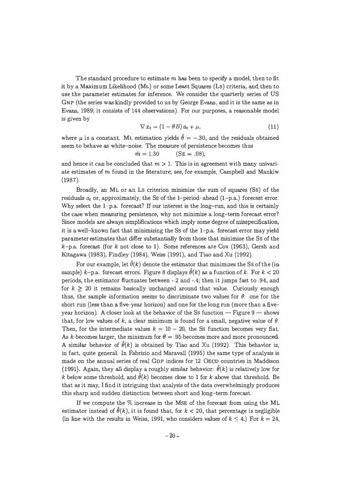
The standard procedure to estimate m has been to specify a model, then to fit it by a Maximum Likelihood (ML) or some Least Squares (Ls) criteria, and then to use the parameter estimates for inference. We consider the quarterly series of US GNP (the series was kindly provided to us by <;;eorge Evans, and it is the same as in Evans, 1989; it consists of 144 observations). For our purposes, a reasonable model is given by

,

V x, = (I - 08) '" + 1', (ll)

where jJ is a constant. ML estimation yields 0 = -.30, and the residuals obtained seem to behave as white-noise. The measure of persistence becomes thus

m = 1.30 (SE = .08),

and hence it can be concluded that m > 1. This is in agreement with many univari­ate estimates of m found in the literature; see, for example, Campbell and Mankiw (1987).

Broadly, an ML or an Ls criterion minimize the sum of squares (SS) of the residuals at or, approximately, the Ss of the I-period-ahead (l-p.a.) forec�t error. Why select the I-p.a. forecast? If our interest is the long-run, and this is certainly the case when measuring persistence, why not minimize a long-term forecast error? Since models are always simplifications which imply some degree of misspecification, it is a well-known fact that minimizing the Ss of the I-p.a. forecast error may yield parameter estimates that differ substantially from those that minimize the Ss of the k-p.a. forecast (for k not close to 1). Some references are Cox (1963), Gersh and Kitagawa (1983), Findley (1984), Weiss (1991), and Tiao and Xu (1992).

For our example, let O(k) denote the estimator that minimizes the Ss of the (in sample) k-p.a. forecast errors. Figure 8 dIsplays ii{k) as a function of k. For k < 20 periods, the estimator fluctuates between -.2 and -.4; then it jumps fast to .94, and for k 2': 20 it remains basically unchanged around that value. Curiously enough thus, the sample information seems�to discriminate two values for 8: one for the short run (less than a five-year horizon) and one for the long run (more than a five­year horizon). A closer look at the behavior of the Ss function - Figure 9 - shows that, for low values of k, a clear minimum is found for a small, negative value of 8. Then, for the intermediate values k = 10 - 20, the Ss function becomes very flat. As k becomes larger, the minimum for 8 = .95 becomes more and more pronounced. A similar behavior of ii{k) is obtained by Tiao and X� (1992). This behavior is, in fact, quite general. In Fabrizio and Maravall (1995) the same type of analysis is made on the annual series of real GDP indices for 12 GEeD countries in Maddison (1991). Again, they all display a roughly similar behavior: ii{k) is relatively low for k below some threshold, and ii{k) becomes close to 1 for k above that threshold. Be that as it may, I find it intriguing that analysis of the data overwhelmingly produces this sharp and sudden distinction between short and long-term forecast.

If we compute the % increase in the MSE of the forecast from using the ML estimator instead of O(k), it is found that, for k < 20, that percentage is negligible (in line with the results in Weiss, 1991, who considers values of k S 4.) For k = 24,

- 20-

use of the ML estimator 6(1) increases the MSE by 14%; for k = 32, this percentage becomes 26%, and for k = 40, it goes up to 31%. Therefore, if our aim is the long­term forecast, it would seem quite inefficient to use as parameter 6(1) = -.30: our MSE may deteriorate by more than 30%.

It is easy to find an explanation for the behavior of 6(k). The good performance of ARIMA models is a result of their ftexibility to adapt their forecast function to the short-run variability. Long-run extrapolation of this short-run flexibility will introduce too much noise in the long-term forecast.

Again, a look at the model components will prove helpful. The IMA{I, 1) model of (8) can be seen as the sum of a trend and an orthogonal white-noise component, where the variance of the noise component can take any value in the interval {O , (I + 0)' V./4); see Box, Hillmer and Tiao (1978). In the trend plus noise decomposition of (8), the forecast of the series is the same as the forecast of the trend. The two models obtained by setting 0 = -.3 and 0 = .95 will imply very different trend components. To compare them, we select the decomposition of (8) that sets the variance of the noise equal to its maximum in the above interval; this is the so-called canonical decomposition, and it maximizes the smoothness of the trend. For the two canonical decompositions corresponding to 8 = -.3 and 9 = .95, the variances of the innovations in the trend component are .423 Va and .001 Va, respectively. When 8 = .95, the trend contains, thus, very little stochastic variability. The two spectra are compared in figure 10. This comparison shows that the trend implied by the model that is optimal for long-term forecasting is very stable, and picks up only very small frequencies. This is a sensible result: when interested in short-term analysis, we look at the month-to-month or quarter-to­quarter forecasts. Thus, for example, the variability of the series associated in the spectrum with the frequency corresponding to a period of 5 years should be a part of the forecast and of the trend. However, if we are forecasting 20 years ahead, the (finite) variance of the series corresponding to a 5-year cycle should not be considered, and hence should not be a part of the trend: in 20 years, the (damped) 5-year cycle has practically disappeared.. This is precisely what figure 10 tells us. When looking at the long run, only movements in the series associated. with very large periods, Le., very small frequencies, are of interest. Figure 11 compares the two (short-term and long-term) trend estimates and the two associated estimates of the noise component. The short-run noise reflects the estimator of a white-noise variable; the long-run noise instead allows for larger effects, since over a long span of time they approximately cancel out.

li the measure of persistence, which attempt� to measure the effect of a shock on the very long-term forecast, is based. on the model optimal for long-term fore-casting, then

m = 1 - .95 = .05.

quite differently from the one obtained. before, and certainly below one. Yet the point is not to claim that this result points towards a business cycle dominated. by

- 21-

demand shocks. The way I read it, the conclusion is that the trend model obtained

in the standard ML estimation-AruMA specification approach only makes sense for

relatively short-tenn analysis. It is with this type of analysis that I have been

concerned in this paper, and it seems to me that the short-term tools we use may

not be appropriate for long-term inference.

- 22 -

XI I : TRANSFER AJNcnON 1.2r---�--�---�--�---�--�-'

------t=\-----(I-------r=r\------7'7\-----f'7\-0.8

0.6

0.4

0.2

°oL---�---u--�l--��--c�L--�� 0.5 1.5 2 2.5 3

Fig. I fI<quency (ralls)

-23-

SPECTRUM: WHITE-NOISE VARIABLE

1.4

1.2

0.8

0.6

0.4

0.2

°o�--��----�----��--��----�----�� 0.5 1.5 2 2.5 3

froquency (rods)

SPECTRUM: SEASONAL COMPONENT IN lliE WHITE NOISE (XII)

1.4

1.2

I - - - - - - - - - - - - - - - - - - - - - - - - - - - - - - - - - - - - - - - - - •• ----.-• • •• ----.--••• ••••••••••••

0.8

0.6

0.4

0.2

oL-____ �� __ �� __ �� ____ L_� __ ��--�� o 0.5 I 1.5 2 2.5 3

Fig. 2 frequency (rods)

- 24 -

SPECTRA: STABLE AND UNSTABLE SEASDNAUTY

, ,

11 " :' :: " " " :: , " " " " " "

:: , " " " , " " " :: " " " " "

:: " " " " " " " 2 " " " ;l " " " " " " " " " " " " "

" " " " " " " , " " " " " " " " " " " 1.5 H " " "

, " " "

.J\ .. " " .' " " " " " " " " " " " .' " " " " .' "

, .' " , .' " "

\j " " " " "

i1 "

.' " " . ' " " "

- " " " . '- .' ' .

0.5

°0�----ble-0�.�5---

al-· --�----�1�.5------�2�----�2�.5�-----3�

unsta season ny .-.....� stable seasonality ......... -y (rads) Fig. 3

- 25-

XII UNDERADJUSTMENT: SERIES AND SEASONAL FILTER

�5r-r---�----�"r---�mr----�----�����

2

1.5

\J 0.5

, U

" " " " " " " " " " " : ' , , "

,

, ,

, , , ,

,

, , , , , ,

°OL-----�0�.5�--���--�1.�5�--�2����2L.5���7;-J series filter Fig. 4 .• mquency (!ads)

XII UNDERADJUSTMENT: SEASONALLY ADJUSTED SERIES 2.5 r-,-----------,-----------------------------,

2

1 .5

0.5

°O�----�----�---��----��----��--�� 0.5 1.5 2 2.5 3 Fig. 4.b

mquency (rads)

- 26-

XII OVERADIUSTMENT: SERIES AND SEASONAL FILTER 2.�r---'r---.r--�...----rrr--�-:rr--�r--�

2

I.� \

0.5

, ! :;.� , " " I , " " " : : . �-----'I '!-_� j j j j

,\----+' ';----�I : : : : I , , I " , . " , , ' . I , " ' ,

, ,

, ..: \. : : °0L-----.�0�.s�--���--�--�--��--���---7�

1 .5 2 2.5 3 senes fiher frequency (!1Ids)

Fig. 5 .• X I I OVERADlUSTMENT: SEASONALLY ADJUSTED SERIES

2.5 r---.-�----

�--__ ---�----�---�....,

2

1.5

O.S

��--�0�.SL---�---�I.S�--�2�--�2.5�L---3� frequency (rads)

Fig. S.b

-27-

2

o.s

· UNSTABLE SEASONAL: SERIES AND AMB SEASONAL FILTER

,

Vi ,

, \l/ , , , , , , , , " , , , \/ ./

, , ,

..

, ,

',.' °o��-.�o�.s--������--��--���--��� '.- - ---' . . . .. '

LS 2 2.S 3 senes tilter n.quency (nds)

Fig. 6.a

UNSTABLE SEASONAL: SEASONALLY ADJUSTED SERIES

2.sr-r---�----�------------�------�----�-'

2

LS

o.S

°0L-----�O�.sL-----��---1�.S-L----�2��--72.�S�----3� frequency (rads)

Fig. 6.b

- 28-

STABLE SEASONAL: SERIES AND SEASONAL FILTER 2.5r__---,---v---�rr_--_.,r--�,.__--..__yr__-�_,

2

STABLE SEASONAL: SEASONALLY ADJUSTED SERIES 2.sr----;-�--�--�--�---�--�.,

2

I.S

0.5

o L-__ � __ � __ �L-_�-L_�� __ �� o 0.5 I.S 2 2.5 3

Fig. 7.b frequency (rads)

- 29-

PARAMETER ESTIMATOR AS A FUNcnON OF THE fORECAST.HORlZON

I ��--�--�--�==�====�==�

0.8

0.6

0.4

0.2

o --------------------------- - - - -. ----- - ------------------------------------- -- --- --

-0.2

-O.4��

-0.6

-0.8

_I L-__ � __ �----�--�--��--�--��--� 5 10 IS 20 25 30 35 40 period-ahead forecast

Fig. 8

5UM OF SQUARES FUNcnON fOR INCREASING fORECASTING HORIZON OO�--�--�--�--�--�--�--�--�--�--�

: '

50 1, .... .......... . ............................... . .................... � ........ . 55(40) ..............

40 "

............. ... . .. . . ............... ..... . .. i

30

20

10

0 -I

. ;

'. 55(12) ./ � � .-�.--- � - - - - - - ----- . - - - - - - -- . - - -.----�-.---- --- .--- . ---.- . - .--. �

- - -.

55(1)

-0.8 -0.6 -0.4 -0.2 0 0.2 0.4 0.6 0.8 Theta

Fig. 9

- 30 -

I

1.4

1.2

0.8

0.6

0.4

0.2

TREND SPECTRUM: SHORT AND LONG TERM MODELS

· · ·

0.5

.

. .

. .

5-year-period fJoquency STuend LT uend

1.5

Fig. 10

2 2.5 3 fJoquency (rods)

- 31 -

8.5 • SHORT RUN TREND

8

7.5

70 20 40 60 80 100 120 140 160

8.5 LONG RUN TREND

8

7.5

7 0 20 40 60 80 100 120 140 160

0.0\ SHORT RUN NOISE

-0.0\ 0 20 40 60 80 100 120 140 160

0.05 LONG RUN NOISE

0

-0.05

-0.1 0 20 40 60 80 100 120 140 160

Fia. 1 1

- 32-

References

BACH, G.L., CAGAN, P.O., FRIEDMAN, M., HILDRETH, C.G., MODIGLIANI, F. and OKUN, A. (1976), Improving the Monetary Aggregates: Repart of the Advisory Committee on Monetary Statistics, Washington, D.C.: Board of Governors of the Federal Reserve System.

BEGUIN, J.M., GOURIEROUX, C. and MONFORT, A. (1980), "Identification of a Mixed Autoregressive-Moving Average Process: The Corner Method" , in O.D. ANDERSON (ed.) Time Senes (Proceedings of a March 1979 Conference), Amsterdam: North-Holland.

BELL, W.K (1984), "Signal Extraction for Nonstationary Time Series" , The Annals of Statistics 12, 2, 646-664.

BELL, W.R. and HILLMER, S.C. (1984), "Issues Involved with the Seasonal Adjust­ment of Economic Time Series" , Journal of Business and Economic Statistics 2, 4, 291-320.

Box, G.E.P., HILLMER, S.C. and TIAO, G.C. (1978), "Analysis and Modeling of Seasonal Time Series" , in A. ZELLNER (ed.), Seasonal Analysis of Economic Time Series, Washington, D.C.: U.S. Dept. of Commerce - Bureau of the Census. 309-334.

Box, G.E.P. and JENKINS, G.M. (1970), Time Senes Analysis: Forecasting and Contro� San Francisco: Holden-Day.

Box, G.E.P. and TIAO, G.C. (1975), "Intervention Analysis with Applications to Economic and Environmental Problems" I Journal of the American Statistical Association 70, 71-79.

BROWN, R.G. (1962), Smoothing, Forecasting and Prediction of Discrete Time Se­ries, New Jersey: Prentice-Hall.

BURMAN, J.P. (1980), "Seasonal Adjustment by Signal Extraction" , Journal of the Royal Statistical Society A, 143, 321-337.

BURRIDGE, P. and WALLIS, K.F. (1984), "Unobserved Components Models for Seasonal Adjustment Filters" , Journal of Business and Economic Statistics 2, 350-359.

CAMPBELL, J.Y. and MANKIW, N.G. (1987), "Permanent and Transitory Compo­nents in Macro-economic Fluctuations" I American Economic Review Proceed­ings 1987, 111-117.

CLEVELAND, W.P. and TIAO, G.C. (1976), "Decomposition of Seasonal Time Series: A Model for the X-ll Program" , Journal of the American Statistical Associa­tion 71, 581-587.

Cox, D.R. (1961), "Prediction by Exponentially Weighted Moving Averages and Related Methods" , Journal of the Royal Statistical Society B, 23, 414-422.

- 33 -

DAGUM, E.B. (1980), "The Xl! ARIMA Seasonal Adjustment Method" , Statistics Canada, Catalogue 12-564E.

DEN BUTTER, F.A.G. and FASE, M.M.G. (1991), Seasonal Adjustment as a Prac­tical Problem, Amsterdam: North-Holland.

ENGLE, R.F. (1978), "Estimating Structural Models of Seasonality" , in A. ZELL­

NER (ed.), Seasonal Analysis of Economic Time Series, Washington, D.C.: U.S. Dept. of Commerce - Bureau of the Census, 281-297.

EVANS, G.W. (1989), "OutPUt and Unemployment Dynamics in the United States: 195()-1985" , Journal of Applied Econometrics 4, 213-237.

FABRIZIO, S. and MARAVALL, A. (1995), IIA Paradox in Long-term Economic Infer­ence from Short-term Time Series Models" , mimeo, Department of E:conomics, European University Institute, Florence.

FERNANDEZ-MACHO, F., HARVEY, A.C. and STOCK, J.H. (1987), "Forecasting and Interpolation Using Vector Autoregressions with Common Trends" , Annales d'Economie et de Statistique 6/7, 279-288.

FINDLEY, D.F. (1984), "On Some Ambiguities Associated with the Fitting of ARMA

Models to Time Series" I Journal of Time Series Analysis 5, 217-227.

FINDLEY, D.F., MONSELL, B., OTTO, M., BELL, W. and PUGH, M. (1992), "To­wards X-12 ARIMA" t mimeo, Bureau of the Census.

GERSCH, W. and KITAGAWA, G. (1983), "The Prediction of Time Series with Trends and Seasonalities" , Journal of Business and Economic Statistics 1, 253-264.

GHYSELS, E. and PERRON, P. (1993), "The Effect of Seasonal Adjustment Filters on Tests for a Unit Root", Journal of Econometrics 55, 57-98.

HARRISON, P.J. and STEVENS, C.F. (1976), "Bayesian Forecasting" , Journal of the Royal Statistical Society B, 38, 205-247.

HARVEY, A.C. (1989), Forecasting, Structurn/ Time Series Models and the Kalman . Filter, Cambridge: Cambridge University Press.

HARVEY, A.C., RUIZ, E. and SENTANA, E. (1992), "Unobserved Component Time Series Models with ARCH Disturbances" , Journal of Econometrics 52, 129-157.

HARVEY, A.C. and TODD, P.H.J. (1983), "Forecasting Economic Time Series with Structural and Box-Jenkins Models: A Case Studi' , Journal of Business and Economic Statistics 1, 4, 299-306.

HILLMER, S.C. and TIAO, G.C. (1982), "An ARIMA-Model Based Approach to Seasonal Adjustment" , Journal of the American Statistical Association 77, 63-70.

HYLLEBERG, S. (1986), Seasonality in Regression, New York: Academic Press.

HYLLEBERG, S: (ed.) (1992), Modeling Seasonality, New York, Oxford University Press.

- 34 -

KENNY, P. and DURBIN, J. (1982), "Local Trend Estimation and Seasonal Adjust­ment of Economic and Social Time Series", Journal of the Royal Statistical SOCiety A, 145, 1-28.

KITAGAWA, G. (1987), "Non-Gaussian State Space Modeling of Nonstationary Time Series", Journal of the American Statistical Association 82, 1032-1063.

LIITERMAN, R.B. (1986), "A Statistical Approach to Economic Forecasting" , Jour­nal of Business and Economic Statistics 4, 1�5.

MADDISON, A. (1991), Dynamic Forces in Capitalist Development: A Long-Run Comparative View, Oxford: Oxford University Press.

MARAVALL, A. (1983), "An AppliCation of Non-Linear Time Series Forecasting" , Journal of Business and Economic Statistics 1, 1.

MARAVALL, A. (1985), "On Structural Time Series Models and the Characterization of Components", Journal of Business and Economic Statistics 3, 4, 350-355.

MARAVALL, A. (1987), "On Minimum Mean Squared Error Estimation of the Noise in Unobserved Component Models" , Journal of Business and Economic Statis­tics 5, 115-120.

MARAVALL, A. (1993), "Stochastic Linear Trends: Models and Estimators" , Journal of Econometrics 54, 1-33.

MARAVALL, A. (1994), "Unobserved Components in Economic Time Series" , EUI Working Paper Eco No. 93/34, Department of Economics, European University Institute. Forthcoming in Pesaran, H., Schmidt, P. and Wickens, M. (eds.), The Handbook of Applied Econometrics, vol. 1, Oxford: Basil Blackwell.

MARAVALL, A. and GOMEZ, V. (1994), "Program SEATS (Signal Extraction in ARIMA Time Series) - Instructions for the User" , EUl Working Paper Eeo No. 94/28, Department of Economics, European University Institute.

MARAVALL, A. and PIERCE, D.A. (1986), "The 'Transmission of Data Noise into Policy Noise in U.S. Monetary Control" , Econometrica 54, 961-979.

MARAVALL, A. and PIERCE, D.A. (1987), "A Prototypical Seasonal Adjustment Model" 1 Journal of Time Series Analysis 8, 177-193.

MILLS, T.e. (1990), Time Series Techniques for Econom.i. .. t� ... Ca.mbridge: Cam­bridge University Press.

MOORE, G.H., Box, G.E.P., KAITZ, H.B., STEPHENSON. J.A. and ZELLNER, A.

(1981), Seasonal Adjustment of the Monetmy A!I9"'9ates: Report of the Com­mittee of Experts on Seasonal Adjustment Tn'hniques, Washington, D.C.: Board of Governors of the Federal Reserve SYSt.C'UL

NERLOVE, M., GRETHER, D.M. and CAllVALHO, J.L. (1979), Analysis of Economic Time Series: A Synthesis, New York: Academic Press.

PIERCE, D.A. (1980), "Data Revisions in Moving Average Seasonal Adjustment Procedures", Journal of Econometrics 14, 1 , 95-114.

-35 -

SHISKIN, J., YOUNG, A.H. and MUSGRAVE, J.C. (1967), "The Xl1 Variant of the Census Method II Seasonal Adjustment Program" . Washington, D.C.: Bureau of the Census, Technical Paper 15.

STOCK, J.H. and WATSON, M.W. (1988), "Testing for Common Trends" , Journal of the American Statistical Association 83, 1097-1107.

TIAO, G.C. and Xu, D. (1992), "Robustness of MLE for Multi-Step Predictions: The Exponential Smoothing Case", Technical Report 117, Statistics Research Center. Graduate School of Business, The University of Chicago.

TSAY, RS. and TIAO, G.C. (1984), "Consistent Estimates of Autoregressive Pa­rameters and Extended Sample Autocorrelation Function for Stationary and Non-Stationary ARMA Models" 1 Journal of the American Statistical Associa­tion 79, 8�96.

WALLIS, K.F. (1974), "Seasonal Adjustment and Relations Between Variables", Journal of the American Statistical Association 69, 18-31.

WEISS, A.A. (1991). "Multi-step Estimation and Forecasting in Dynamic Models" , /ournal of Econometrics.48, 135-149.

WHITTLE, P. (1963), Prediction and Regulation by Linear Least-Square Methods, London: English Universities Press.

WINTERS, P.R (1960), "Forecasting Sales by Exponentially Weighted Moving Av­erages" , Management Science 6, 324-342.

WODEHOUSE, P.G. (1981), Wodehouse on Wodehouse, Penguin Books.

- 36-

WORKING PAPERS (1) 9310 Amparo Ricardo Ricardo: Series hist6ricas de contabilidad nacional y mercado de trabajo

para Ja CE y EEUU: 1%0-1991.

9311 Fernando Restoy and G. Michael Rockinger: On stock market returns and returns on in­vestment.

9312 JesUs Saurina Salas: Indicadores de solvencia bancaria y contabilidad a valor de mercado.

9313 Isabel Argim6n, Jose Manuel Gonz8)ez-Paramo, Maria JesUs Martin and Jose Maria Roldan: Productivity and infrastructure in the Spanish economy. (The Spanish original of this publi· cation has the same number.)

9314 Fernando Ballabriga, Miguel Sebastian and Javier Valles: Interdependence of EC econo­mies: A VAR approach.

9315 Isabel Argimon y Mo- JesUs Martin: Serle de t<stock» de infraestructuras del Estado y de las Administraciones PUblicas en Espana.

9316 P. Martinez Mendez: Fiscalidad, tipos de interes y tipo de cambio.

9317 P. Martinez Mendez: Efectos sobre la paUlica econ6mica espanola de una fiscalidad distor­sionada por la inflaci6n.

9318 Pablo Antolin and Olympia BoYer: Regional Migration in Spain: The effect of Personal Characteristics and of Unemployment, Wage and House Price Differentials Using Pooled Cross-Sections.

9319 Samuel Bentolila y Juan J. Dolado: La contrataci6n temporal y sus efectos sobre la compe­titividad.

9320 Luis Julian Alvarez, Javier Jareno y Miguel Sebastian: Salarios publicos, salarios privados e inflaci6n dual.

9321 Ana Revenga: Credibility and inflation persistence in the European Monetary System. (The Spanish original of this publication has the same number.)

9322 Maria Perez Jurado and Juan Luis Vega: Purchasing power parity: An empirical analysis. (The Spanish original of this publication has the same number.)

9323 Ignacio Hernando y Javier Valles: Productividad sectorial: comportamiento ciclico en la economfa espanola.

9324 Juan J. Dolado, Miguel Sebastian and Javier Valles: Cyclical patterns of the Spanish eco­nomy.

9325 Juan Ayuso y Jose Luis Escri"': La evoluci6n del control monetario en Espana.

9326 Alberto Cabrero Bravo e Isabel Sanchez Garda: M�todos de predicci6n de los agregados monetarios.

9327 Cristina Mazon: Is profitability related to market share? An intra-industry study in Spanish manufacturing.

9328 Esther Gordo y Pilar L'Hotellerie: La competitividad de la industria espanola en una pers­pectiva macroecon6mica.

9329 Ana Buisan y Esther Gordo: El saldo comercial no energetico espanol: determinantes y amUisis de simulaci6n (1964-1992).

9330 Miguel Pellicer: Functions of the Banco de Espana: An historical perspective.

9401 Carlos Ocana, Vicente Salas y Javier Valles: Un analisis empfrico de la financiaci6n de la pequena y mediana empresa. manufacturera espanola: 1983-1989.

9402 P. G. Fisher and J. L. Vega: An empirical analysis of M4 in the United Kingdom.

9403 J. Ayuso, A. G. Haldane and F. Restoy: Volatility transmission along the money market yield curve.

9404 Gabriel Quiros: El mercado britanico de deuda publica.

9405 Luis J. Alvarez and Fernando C. 8aUabriga: BVAR models in the context of cointegration: A Monte Carlo experiment.

9406 Juan Jose DoIado, Jose Manuel GonUlez-P4nuno y Jose M: Roldan: Convergencia eco­n6mica entre las provincias espano!as: evidencia empirica (1955-1989).

9407 Angel Estrada e Ignado Hernando: La inversi6n en Espana: un analisis desde el lado de la oferta.

9408 Angel Estrada Garda, M." Teresa Sastr< de Miguel y Juan Lois Vega Croissier: EI meca­nismo de transmisi6n de los tipos de interes: el caso espano!.

9409 PUar Garcia Perea y Ramon Gomez: Elaboraci6n de series hist6ricas de empleo a partir de la Encuesta de Poblaci6n Activa (1964-1?92).

9410 F. J. Saez Perez de Ia Torre, J. M: Sanchez Saez y M: T. Sastte de Miguel: Los mercados de operaciones bancarias en Espana: especializaci6n productiva y competencia.

9411 Olympia Bover and Angel Estrada: Durable consumption and house purchases: Evidence from Spanish panel data.

9412 Jose Vliials: Building a Monetary Union in Europe: Is it worthwhile, where do we stand, and where are we going? (The Spanish original of this publication has the same number.)

9413 Carlos Cbuli&: Los sistemas financieros nacionales y el espacio financiero europeo.

9414 Jose Luis Escriva and Andrew G. Haldane: The interest rate transmission mechanism: Sec­toral estimates for Spain. (The Spanish original of this publication has the same number.)

9415 Mo- de los Llanos Matea y Ana Valentina Regil: Metodos para la extracci6n de sefiales y para la trimestralizaci6n. Una aplicaci6n: Trimestralizaci6n del deflactor del consumo pri­vado nacional.

9416 Jose Antonio Cuenca: Variables para el estudio del sector monetario. Agregados moneta­rios y crediticios, y tipos de interes sinteticos.

9417 Angel Estrada y David L6pez·Salido: La relaci6n entre el consumo y la renta en Espana: un modelo empfrico con datos agregados.

9418 Jose M. Gormilez Mioguez: Una aplicaci6n de los indicadores de discrecionalidad de la poHtica fiscal a los paises de la UE.

9419 Juan Ayuso, Maria Perez JUl'ado and Fernando Restoy: ]s exchange rate risk higher in the E.R.M. after the widening of fluctuation bands? (The Spanish original of this publication has the same number.)

9420 Simon MilDer and David. Metcalf: Spanish pay setting institutions and performance outcomes.

9421 Javier Santillan: El SME, los mercados de divisas y la transici6n bacia la Uni6n Monetaria.

9422 Juan Luis Vega: Is the ALP long-run demand function stable? (The Spanish original of this publication has the same number.)

9423 Gabriel QuirOs: EI mercado italiano de deuda publica.

9424 Isabel Argimoo, Jose Manuel Gonzalez-Paramo y Jose Maria Rold8n: ]nversi6n privada, gasto publico y efecto expulsi6n: evidencia para el caso espano!.

9425 Charles Goodhart and Jose VliiaIs: Strategy and tactics of monetary policy: Examples from Europe and the Antipodes.

9426 CanneD MeleOo: Estrategias de politica monetaria basadas en el seguimiento directo de objetivos de inflaci6n. Las experiencias de Nueva Zelanda, Canada, Reino Unido y Suecia.

9427 Olympia Bover and Manuel Arellano: Female labour force participation in the 1980s: the case of Spain.

9428 Juan Maria Peiialosa: The Spanish catching·up process: General detenninants and contri· bution of the manufacturing industry.

9429 Susana Nunez: Perspectivas de los sistemas de pagos: una refiexi6n cntica.

9430 Jose'VJ.iials: i,Es posible la convergencia en Espana?: En busca del tiempo perdido.

9501 Jorge Bbizquez y Miguel Sebasti8n: Capital publico y restricci6n presupuestaria guberna· mental.

9502 Ana Buisan: Principales determinantes de los ingresos por turismo.

9503 Ana Buis8n y Esther Gordo: La protecci6n nominal como factor determinante de las im· portaciones de bienes.

9504 Ricardo Mestre: A macroeconomic evaluation of the Spanish monetary policy transmis· sion mechanism.

9505 Fernando Restoy and Ana Revenga: Optimal exchange rate flexibility in an economy with intersectoral rigidities and nontraded goods.

9506 Angel Estrada and Javier Valles: Investment and financial costs: Spanish evidence with pa· nel data. (The Spanish original of this publication has the same number.)

9507 Francisco Alonso: La modelizaci6n de la volatilidad del mercado bursatil espanol.

9508 Francisco Alonso y Fernando Restoy: La remuneraci6n de la volatilidad en el mercado es· panol de renta variable.

9509 Fernando C. BaDabriga, Miguel SebastUin y Javier VaDes: Espana en Europa: asimetnas reales y nominales.

9510 Juan Carlos Casado, Juan Alberto Campoy y Carlos ChuJiB: La regulaci6n financiera espa· nola desde la adhesi6n a la Uni6n Europea.

9511 Juan Luis Diaz del Hoyo y A. Javier Prado Dominguez: Los FRAs como guias de las expec· tativas del mercado sobre tipos de interes.

9512 Jose M.- Sanchez Saez y Teresa Sastre de Miguel: i,Es el tamano un factor explicativo de las diferencias entre entidades bancarias?

9513 Juan Ayuso y Soledad Nunez: i,Desestabilizan los activos derivados el mercado al conta· do?: La experiencia espanola en el mercado de deuda publica.

9514 M: Cruz Manzano Frias y M: Teresa Sastre de Miguel: Factores relevantes en la detenni· naci6n del margen de explotaci6n de bancos y cajas de ahorros.

9515 Fernando Restoy and Philippe Well: Approximate equilibrium asset prices.

9516 Gabriel QuirOs: El mercado frances de deuda publica.

9517 Ana L. Revenga and Samuel Bentolila: What affects the employment rate intensity of growth?

9518 Ignacio Iglesias Aralizo y Jaime Esteban Velasco: Repos y operaciones simultaneas: estu-dio de la nonnativa.

9519 Ignacio Fuentes: Las instituciones bancarias espanolas y el Mercado Unico.

9520 Ignacio Hernando: Politica monetaria y estructura financiera de las empresas.

9521 Luis JuIi8n Alvarez y Miguel Sebastian: La inflaci6n latente en Espana: una perspectiva macroecon6mica.

9522 Soledad Nunez Ramos: Estimaci6n de la estructura temporal de los tipos de interes en Espana: elecci6n entre metodos alternativos.

9523 Isabel Argimon, Jose M. Gonz8J.ez-P1iramo y Jose M.' Roldan Alegre: Does public spen­ding crowd out private investment? Evidence from a panel of 14 OECD countries.

9524 Luis Julian Alvarez, Fernando C. Ballabriga y Javier Jareiio: Un modelo macroeconome­trico trimestral para la economia espanola.

9525 Aurora Alejano y Juan M: Penalosa: La integraci6n financiera de la economia espanola: efectos sobre los mercados financieros y la politica monetaria.

9526 Ramon Gomez Salvador y Juan J. Dolado: Creaci6n y destrucci6n de empleo en Espana: un amilisis descriptivo con datos de la CSSE.

9527 Santiago Fernandez de Lis y Javier Santillan: Regimenes cambiarios e integraci6n moneta­ria en Europa.

9528 Gabriel Quiros: �ercados financieros ale manes.

9529 Juan Ayuso Huertas: Is there a trade-off between exchange rate risk and interest rate risk? (The Spanish original of this publication has the same number.)

9530 Fernando Restoy: Determinantes de la curva de rendimientos: hip6tesis expectacional y primas de riesgo.

953/ Juan Ayuso and Maria Perez Jurado: Devaluations and depreciation expectations in the EMS.

9532 Paul Schulstad and Angel Serrat: An Empirical Examination of a Multilateral Target Zone Model.

9601 Juan Ayuso, Soledad Nunez and Maria Perez-Jurado: Volatility in Spanish financial markets: The recent experience.

9602 Javier Andres e Ignacio Hernando: iC6mo afecta la inflaci6n al crecimiento econ6mico? Evidencia para los paises de la OCDE.

9603 Barbara Dluhosch: On the fate of newcomers in the European Union: Lessons from the Spanish experience.

9604 Santiago Fernandez de Lis: Classifications of Central Banks by Autonomy: A comparative analysis.

9605 M: Cruz Manzano Frias y Sofia Galmes Belmonte: Politicas de precios de las entidades de credito y tipo de c1ientela: efectos sobre el mecanismo de transmisi6n.

9606 Malte Kruger: Speculation. Hedging and Intermediation in the Foreign Exchange Market.

9607 Agustin Maravall: Short-Term Analysis or Macroeconomic TIme Series.

( I ) Previously published Working Papers art! listed in the Banco de Espana publications catalogue.

Queries should be addressed to: Banco de Espana Seccion de Publicaciones. Negociado de Distribution y Gestion

Telephone: 338 51 80 Alcala, 50. 28014 Madrid