UNIVERSITÀ DEGLI STUDI DI MILANO Ph.D SCHOOL IN COMPUTER SCIENCE (C0R) DEPARTMENT OF INFORMATION TECHNOLOGIES Ph.D. COURSE IN COMPUTER SCIENCE - XXII CICLE Ph.D. THESIS ADVANCED COMPUTATIONAL METHODS FOR THE INVESTIGATION OF BIOPHYSICAL PROPERTIES OF MACROMOLECULAR PROTEINS SILVIA FIORENTINI Supervisor Prof.ssa RITA PIZZI Co-Supervisor Prof. MASSIMO PREGNOLATO Director of the Ph.D. School Prof. ERNESTO DAMIANI A.A. 2010/2011 1
Transcript
UNIVERSITÀ DEGLI STUDI DI MILANO
Ph.D SCHOOLIN COMPUTER SCIENCE (C0R)
DEPARTMENTOF INFORMATION TECHNOLOGIES
Ph.D. COURSEIN COMPUTER SCIENCE - XXII CICLE
Ph.D. THESIS
ADVANCED COMPUTATIONAL METHODS FOR THE
INVESTIGATION OF BIOPHYSICAL PROPERTIES OF
MACROMOLECULAR PROTEINS
SILVIA FIORENTINI
Supervisor Prof.ssa RITA PIZZI
Co-Supervisor Prof. MASSIMO PREGNOLATO
Director of the Ph.D. School Prof. ERNESTO DAMIANI
A.A. 2010/2011
1
INDEX
ABSTRACT 5
AIM OF THE WORK 8
INTRODUCTION 10
1.1 Introduction on Bioinformatics 11
1.1.1 Definition 11
1.1.2 Structural Bioinformatics 14
1.1.3 Molecular Dynamics 20
1.2 Computational Methods: Molecular Dynamics 24
1.2.1 Amber 24
1.2.2 Molecular Workbench 25
1.2.3 Ascalaph 26
1.3 Computational Methods: Softcomputing 27
1.3.1 Kernel Methods 28
1.3.2 Bayesian Networks 30
1.3.3 Hidden Markov Models 31
1.3.4 Support Vector Machines 32
1.3.5 Genetic Algorithms 33
1.3.6 Artificial neural networks 36
MATERIALS 44
2.1 Microtubules and Tubulin 45
2.2 Microtubules and Tubulin Preparation 49
2.3 Buckyballs 49
2.4 Nanotubes 512
2.5 Comparison between Microtubules and Nanotubes 53
2.6 Hypothesis about Quantum Properties of MTs 54
METHODS 59
3.1 Experimental and Theoretical Methods 60
3.1.1 Fluorescence 60
3.1.2 Resonance 63
3.1.3 Birefringence 65
3.1.4 Superradiance 68
3.2 Computational ad hoc Methods 73
3.2.1 Molecular Dynamics 73
3.2.2 Dynamic System Evolution 76
3.2.3 ANN Processing: the ad hoc ITSOM implemented 92
RESULTS 93
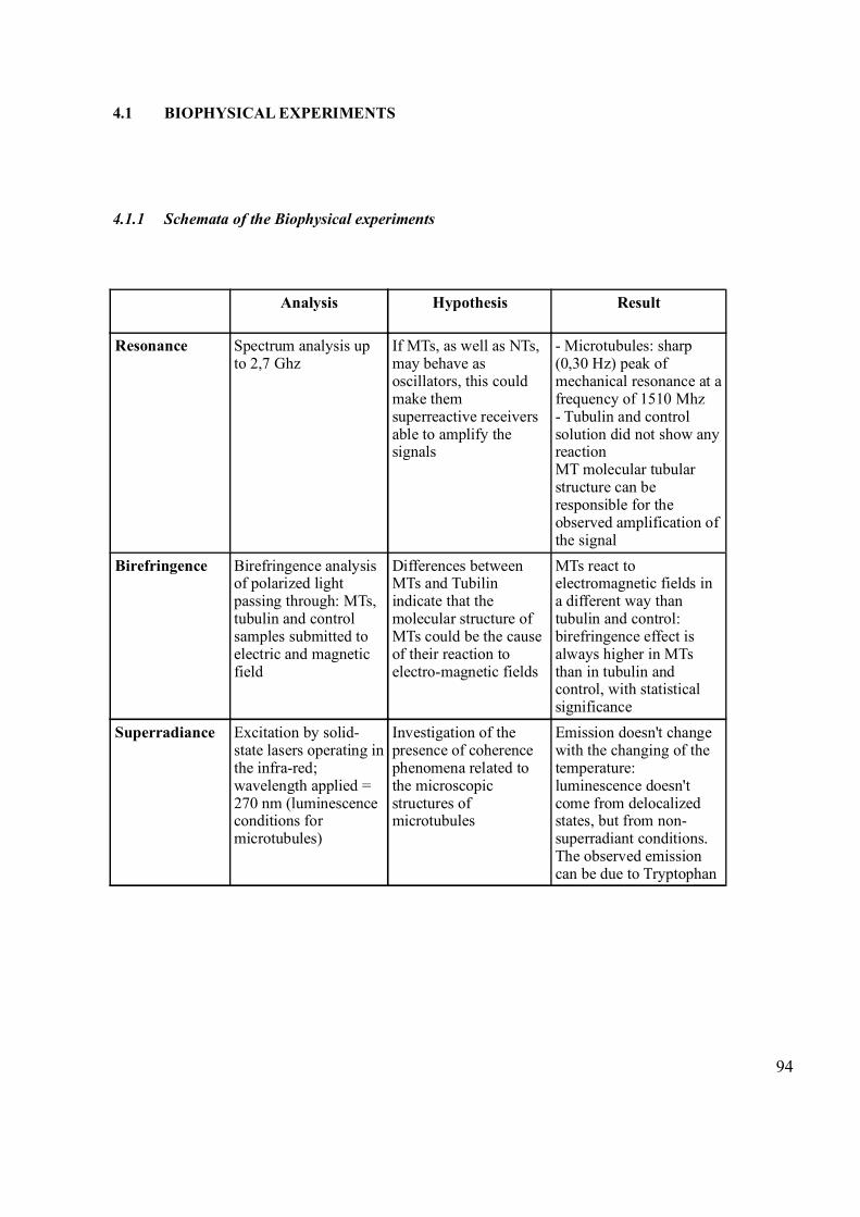
4.1 Biophysical Experiments 94
4.1.1 Schemata of the Biophysical experiments 94
4.1.2 Resonance Experiment 95
4.1.3 Birefringence Experiment 96
4.1.4 Superradiance Experiment 102
4.2 Computational Analysis 106
4.2.1 Analysis of Superradiance results with Molecular Workbench 106
4.2.2 Molecular Dynamics for interpretation of experimental results 114
4.3 Artificial Neural Networks 119
DISCUSSION 125
3
CONCLUSIONS AND FUTURE TRENDS 129
APPENDIX 132
Software for secondary structure prediction based on neural networks 133
REFERENCES 137
4
ABSTRACT
5
The focus of this thesis is the application of novel advanced computational methods to
specifically interpret data from biophysical experiments performed on particular
macromolecular structures: microtubules and tubulin.
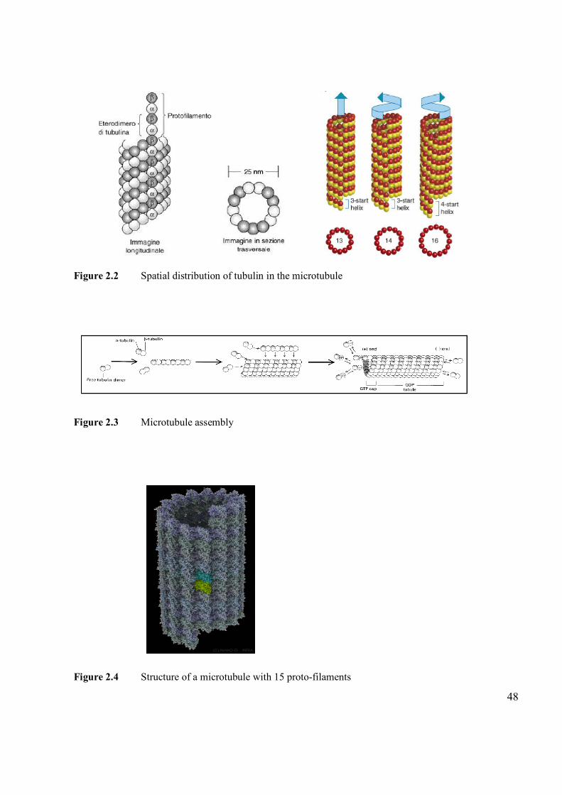
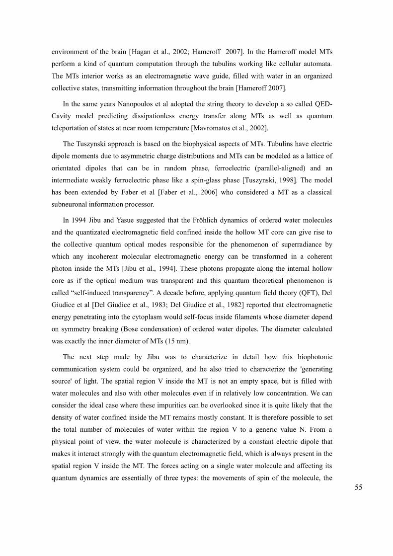
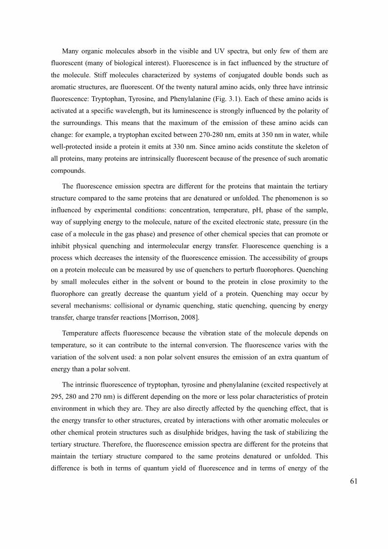
Microtubules (MTs) are macromolecular protein assemblies with well-known key roles in
all eukaryotic cells. It is assumed however that they also have an important role in intercellular
communication over long distances, especially in the network of neurons. This feature may
explain mechanisms little-known so far, such as the immediate involvement of the entire
immune system to local damage, or may help to clarify some unsolved questions about the
mind-body problem.Taking into account the connection between structural and physical
properties in Carbon Nanotubes (CNTs) and their structural similarity to MTs, our basic
assumption in this research was that when tubulin and MTs show different biophysical
behaviours, this should be due to the peculiar dynamical organization of MTs.
In order to investigate the biophysical properties of the macromolecular structure object of
this study, microtubules and tubulin, an innovative approach has been applied:
- ad hoc experimental procedures have been prepared, from which the experimental data
have been obtained;
- ad hoc computational methods have been developed specifically to interpret the
experimental data.
The theoretical assumptions of the computational methods used are based on the theory of
dynamic evolution of complex systems and on the properties originating from their self-
organization capacity.
The physical properties of birefringence, resonance and superradiance were measured, and
data from biophysical experiments were analysed using ad hoc computational methods:
dynamic simulation of MTs and tubulin was performed, and their level of self-organization was
evaluated using artificial neural networks. The results from dynamic simulations were submitted
to two different self-organizing artificial neural networks: the first one for the evaluation of
specific parameters, and the second one for the evaluation of dynamic attractors. We developed
a procedure that processes in the form of attractors the series of winner neurons resulting from
the output of the neural network.
Both tubulin and MTs show dynamic stability, but only MTs exhibit a significant behaviour
in presence of electric field, in the direction of a stronger structural and spatial organization. The
Artificial Intelligence approach supports the experimental evidences at the microscopic level,
allowing a more correct and accurate interpretation of the results.
6
The research we carried out reveals the existence of a dynamic and organized response of
MT to electromagnetic fields, which could justify their role in receiving and transmitting
information even at long distances. The innovative computational methods implemented in this
work revealed to be very useful for the dynamic analysis of such complex structures.
7
AIM OF THE WORK
8
This research project aims at the understanding of the anomalous properties of particular
biological structures, called microtubules, by means of the synergistic use of computational
methods for the analysis of data from biophysical experiments.
In the study of the physical properties and dynamic organization of MTs compared with
those of CNTs, it is desired to search and analyze a possible reaction to the electromagnetic
field, observing any ability of MTs to absorb or emit like antennas. The MTs, as well as CNTs,
may behave as oscillators, and this could make them superreactive receivers able to amplify the
signals.
We carried out a set of in vitro experiments on MTs and tubulin, in order to evaluate if their
different structures could be responsible of different biophysical behaviours and properties.
Then we explored the possible meaning of the obtained findings by simulating and comparing
the dynamic evolution of MTs, tubulin and CNTs. Molecular Dynamics and physico-chemical
simulations were performed, in order to analyse the dynamic evolution of the physical system at
the atomic and molecular level.
To study the evolution of the dynamic organization of the examined structures under the
influence of electromagnetic fields two different procedures based on Artificial Neural
Networks (ANNs) models were developed and applied. The coordinate values xyz of the
molecules after dynamic simulation were used as input value for neural networks, whereas the
output of the ANNs was analysed by using the occupancy – conflicts method and the attractor’s
method.
It has been possible to justify the experimental results in light of structural and dynamic
models, highlighting the actual existence, so far only a hypothesis, of substantial effects of
electromagnetic fields on the dynamic evolution of microtubules. As prevoiusly discussed by
Albrecht-Buehler, radial microtubules around the centrosome show reduced stability in response
to pulsating near-infrared signals of 1 s pulse length (Albrecht-Buehler, 1998). The results are
consistent with the interpretation that the centrosome responded to the light by sending signals
along its radial array of microtubules whose stability was then altered.
Evidence of anomalous behaviour of microtubules in the presence of electromagnetic field
and its explanation in terms of dynamic organization is an important step towards the
understanding of the important role of microtubules in cell communication over long distances,
since the long-range intracellular communication may explain some of the biological
mechanisms still unsolved, both at neuronal and immune system level.
9
1. INTRODUCTION
10
1.1 INTRODUCTION TO BIOINFORMATICS
1.1.1 Definition
Bioinformatics aims to describe biophysical and biological phenomena from the numerical
and statistical point of view, by applying computational methods to problems of biophysics and
biology.
In the last years the use of increasingly advanced technologies for the study of biological
systems has resulted in huge amounts of data and information, which is greatly amplified
because these data represent only very small pieces of larger and more complex systems. All
this information represents an invaluable resource for understanding the molecular mechanisms
underlying the functioning of cells and organisms, but on the other hand it generates serious
issues in terms of their management and interpretation. Because of this reason, along with
molecular biology a new branch of computer science has developed: bioinformatics.
The field of bioinformatics is growing rapidly for several reasons. First of all, it is necessary
to create, manage and maintain specialized databases able to store the huge amount of data that
modern biological research produces thanks to the recent technological progress. Moreover, in
addition to archiving data, it is fundamental to automatically mine information from the
databases. Bioinformatics is therefore very helpful for biological and biotech research, which
can be directed and focused, with considerable reduction in the costs of implementation.
Bioinformatics focuses on:
- Providing statistical models valid for the interpretation of data from experiments in molecular
biology and biochemistry, to identify trends and numerical laws;
- Creating new models and mathematical tools for analyzing DNA, RNA and proteins to create
a set of knowledge concerning the frequency of relevant sequences, their development and
possible function;
- Organizing a global knowledge on genome and proteome into suitable databases in order to
make such data accessible to all, and optimizing the algorithms for data searching and mining.
The term bioinformatics is also used for the development of computational algorithms that
mimic biological processes, such as neural networks or genetic algorithms. The availability of
entire genome sequences from different species makes it possible to investigate the function of
conserved non-coding regions of DNA. The distribution of data in coding (genes) and non-
coding sequences and their subsequent organization in special database for DNA and proteins
11
are a key objective of bioinformatics (Li et al., 2006.). The development of these databases
allows the realization of software for the analysis of nucleotide (DNA and RNA) and protein
sequences, such as FASTA (Pearson et al., 1988) and PSI-BLAST (Altschul et al., 1997). These
tools greatly facilitate the search for homologous sequences and the understanding of their
mutual relations, thus causing an increase of functionally annotated database. There are
bioinformatics tools, such as Genebuilder, Grail, GenScan, GenesH, able to predict putative
biological functions with a variable degree of accuracy: splicing sites, exons, introns, coding
regions, promoters, polyadenylation sites, etc.
With modern so-called "high-throughput” technologies of molecular biology it is possible to
determine gene expression of thousands of genes simultaneously in a single experiment: this is
called the microarray technology (Eisen et al., 1999; Schena et al., 1995; Hanai et al., 2006).
The microarray technology makes use of bioinformatics in several phases: experimental design,
annotation of sequences, image and raw data acquisition, data analysis, database mining (Olson
et al., 2006). The gene annotation software is web based and allows the viewing, editing and
storing of annotations for both prokaryote and eukaryote genomes. The identification of genes
and their assignment to functional families is based on several genomic analysis tools: Gene
Ontology (GO) classification (Boyle et al., 2004), search for sequences by BLAST, MIAME
(Minimal Information About a Microarray Experiment), MAGE-ML (European Bioinformatics
Institute), GeneX-Lite (National Center for Genome Resources), Manatee (TIGR), GenMapp
(University of California at San Francisco). Image acquisition and analysis is a crucial step in
microarray analysis. Dedicated software processes the fluorescence data from the array image:
TIFF files created by scanners are read and, through the semi-automatic construction of a grid,
the area of the slide containing the spots is defined. Two different methods for segmentation
(histogram method and Otsu segmentation) are available to define the boundary between each
spot and local background. The intensity of the spots is counted as integral of not-saturated
pixels, or by calculating the value of the median or the average of the spot. Local background
subtraction is then applied to each value. Microarray data can be analyzed using different ap-
proaches (Claverie et al., 1999). Data analysis software consists essentially of a combination of
tools aimed at clustering, pattern discovery, Gene Ontology search, analysis and visualization of
gene expression data and of other genomic data. This also allows the linking of data obtained
from tools and external databases. The search for functional cluster is usually performed
through correlation with database of functional annotations (e.g. Gene Ontology).
Database mining techniques are defined as a series of computational tools for exploring and
analyzing large amounts of data in order to extract characteristic and persistent motifs (patterns)
and rules. The algorithms for database mining are derived from the fields of statistics, pattern
12
recognition, artificial intelligence and signal analysis; they use information directly obtained
from data to create empirical models able to describe the behaviour of a complex system. In
gene expression profiles data mining techniques are a useful tool for identifying and isolating
specific patterns of expression, which represent genetic fingerprinting of a specific
physiological state. Data analysis of cDNA arrays is usually based on the synergistic use of
hypothesis testing and of systems for knowledge discovery. Hypothesis testing methods are
basically top-down approaches that scan the data seeking experimental confirmation to
previously formulated hypotheses. The knowledge discovery, instead, can be considered as a
bottom-up approach where the data itself provide the information necessary for the formulation
of new hypotheses. A crucial aspect of the application of these procedures is the identification of
all those genes that show high activity in a particular physiological state. These active genes,
and their network of relationship, can be identified by using techniques such as Mean
Hypothesis Testing (MHT), Cluster Analysis (CA) Principal Component Analysis (PCA) and
Decision Tree (DT).
The genome sequencing projects and the other high-throughput approaches generate
thousands of new protein sequences from different organisms. Bioinformatics is therefore
essential for proteomic studies aimed at assigning a function to each protein: it can establish
similarity correlations with already characterized proteins by homology analysis and
evolutionary inference, and rationalize the function from the structural point of view, using
experimental structural data or model-derived data. By looking separately at sequences or
protein folding, little can be said about the function. Instead, taking into consideration both
sequences and structures together, the emerging conserved patterns, called motifs, provide
important functional information.
Another field strongly implemented by using bioinformatics is that of combinatorial
chemistry: in vitro chemical synthesis of hundreds of modified molecules and their subsequent
tests of interaction with potential pharmacological targets has been increased by virtual 3D
reconstructions of molecules and their in silico screening searching for the best pharmacological
ligands. Only molecules with high score of interaction are then synthesized and tested in vitro,
with significant cost savings.
Bioinformatics also plays an important role in the field of meta-analysis. Meta-analysis is
the statistical procedure for combining data from multiple studies. It is useful for the
identification of homogeneous sets of information across different data, for example microarray
studies on different species or different treatments. It allows a more objective appraisal of the
evidence than traditional narrative reviews, provides a more precise valuation of data (for
example the estimate of a treatment effect), and may explain heterogeneity between the results
13
of individual studies.
A useful tool for meta-analysis is represented by Pointillist, which is a set of four software
programs (Data Manager, Data Normalizer, Significance Calculator, Evidence-Weighted
Inferer) for inferring the set of elements affected by a perturbation of a biological system based
on multiple types of evidence. The inference is based on a weighted statistical method, in which
each evidence type is given a distinct trustworthiness weight. The method is robust against
missing and inconsistent data. Pointillist is written in Java, and is based on the ISB Java library.
All four programs read data files in which the columns are evidence types and the rows are
elements of the system (e.g., genes or proteins). The Data Manager is used for data sub-
selection and averaging. The Data Normalizer is (optionally) used to perform normalization of
microarray expression data. The Significance Calculator is used to obtain P-values for
measurements based on a distribution of observations for negative control(s). Both parametric
and nonparametric methods can be used to obtain the P-values. The Evidence-Weighted Inferer
is used to combine the P-values for observations of different evidence types, and obtain a
consensus P-value for each element of the system. The elements are classified into the "null
hypothesis" (likely unaffected) set, and the set of likely affected elements, using an iterative
procedure (Hwang et al., 2005).
1.1.2 Structural Bioinformatics
Structural Bioinformatics is the field of bioinformatics aiming at the analysis and prediction
of the morphology and structure of biological macromolecules such as proteins and nucleic
acids. Macromolecules are fundamental for all the functions of the cell, and it is only by taking
appropriate three-dimensional shapes that proteins and sub-cellular components can perform
their functions.
Proteins are one of the fundamental macromolecules forming the cells. One of the central
topics of modern research in molecular biology, biochemistry and biophysics is the
understanding of how these functions are related to the molecular structure. Proteins are linear
polymers made of hundreds of elementary units, the amino acids, characterized by a carboxy-
terminal end (acid) and an amino terminal end (basic) and exist in nature in 20 different
varieties. The study of the structural organization of proteins takes place at 4 different levels:
- Primary structure: it corresponds to the sequence of the amino acids and to the position of
disulfide bonds, if any, and therefore reflects all the covalent bonds of a protein.14
- Secondary structure: it refers to the space conformation of adjacent amino acid residues in
linear sequence. Some of these steric connections are regular and give rise to periodic
structures, such as α-helix and β-sheet. When steric relationships are not regular, they are called
random-coil.
- Tertiary structure: it is related to the position in the space (3D coordinates) of amino acid
residues that are far apart in the linear sequence.
- Quaternary structure: proteins that contain more than one polypeptide chain have an
additional level of structural organization: each polypeptide chain is called a subunit and
quaternary structure refers to the spatial arrangement of these subunits into complexes.
Predicting the three-dimensional arrangement of proteins, namely their tertiary structure,
from the linear sequence of the component amino-acids (primary structure), has become a topic
of great relevance since the techniques of molecular biology (recombinant DNA) are able to
collect information on primary structure at a much higher rate than traditional spectroscopic
techniques (X-ray diffraction, NMR, etc.) respectively do for the three-dimensional structures.
Before the advent of structural genomics the main interest in solving the structure of a
protein was to understand and better analyse the determinants of its function, which was already
assigned after biochemical or genetic experiments were performed. The increasing number of
fully sequenced genomes together with the progress in homology modelling of protein
structures shifted the interest on characterizing the largest number of different folds to have the
best possible sampling of structure space. The rationale is that, as more and more structural
folds are characterized, homology modelling of an increasing number of proteins should
become possible and more reliable. In light of this goal, targets for structure determination are
selected among proteins with very low sequence identity to proteins of known structure. As a
consequence, a large number of structures belong to proteins of unknown function. This fact has
enormously increased the interest in computational methods for structure-guided functional
inference. Structural comparison methods are potentially able to identify very distant
evolutionary relationships between proteins. Moreover, only structural data makes the
identification of independently evolved functional sites possible [Via et al., 2000; Ausiello et al.
2007; Gherardini et al. 2007].
A first group of functional annotation methods uses a comparative approach searching for
common features between the query protein and some database of protein structures; other
methods analyse the physicochemical characteristics of a protein surface to identify patches that
have features (e.g. shape, electrostatic properties, etc.) characteristic of functional sites.
15
Comparative Approaches are similar to sequence comparison methods, and can be
classified as global or local. Global comparison algorithms are mainly used in protein structure
classification to identify evolutionary links between distant homologues. They can also be used
for function prediction but the relationship between fold and function is extremely complex and
numerous examples are known of folds hosting a great variety of functions [Gerlt et al., 2001].
It should indeed be noted that the function of a protein usually depends more on the identity and
location of a few residues comprising the active site than on the overall fold. Therefore, the
usefulness of global comparison methods is essentially indirect and lies in their capability of
identifying remote homology relationships. In order to directly analyse and compare the
residues effectively involved in protein function, local structural comparison methods have been
developed. Local structural comparison refers to the possibility of detecting a similar 3D
arrangement of a small set of residues, possibly in the context of completely different protein
structures. Such algorithms can either compare two entire protein structures in search for local
similarities, without any a priori assumption, or use a pre-defined structural template to screen a
structure. A template represents the spatial arrangement of the residues involved in some
biochemical function and can be regarded as a 3D extension of the linear sequence motif
concept. In general, local structural comparison methods can also be used to search for
templates. The JESS [Barker et al., 2003] algorithm gives the possibility of expressing the
template as a set of high-level constraints of arbitrary nature. The program DRESPAT
[Wangikar et al., 2003] uses a graph theoretic method to enumerate patterns recurring in a set of
structures. The problem of assessing the statistical significance of a local structural similarity is
complex. The biggest gap, in terms of statistical analysis, between sequence comparison and
structure comparison is that in the latter case there is no universally accepted random model that
can be used as a basis for significance assessment.
Since no definitive way exists to identify statistically significant matches, it is very
important to integrate structural comparison methods with detailed functional annotations in
order to steer the search towards functionally significant residues. When a match between two
proteins involves residues for which functional annotations are available, one can more easily
derive clues about the significance of a correspondence even in the absence of a rigorous
statistical framework. Various tools have been developed to ease the functional annotation of
protein structures.
The E-MSD structure database [Boutselakis et al., 2003] aggregates an enormous amount of
functional information about protein structures, coming from a variety of sources.
SPICE [Prlic et al., 2005] is a graphical client for the DAS system [Dowell et al., 2001] that
allows annotations from different laboratories hosting a DAS server to be mapped and displayed
16
on the structure of a protein of interest.
The pdbFun webserver [Ausiello, Zanzoni et al., 2005] integrates functional annotations at
residue level with the Query3d local structural comparison method so that the residues to be
used in a comparison run can be selected on the basis of functional information. [Ausiello, Via
et al., 2005].
SWISS-MODEL is an environment for comparative protein modelling. It consists of
SWISS-MODEL, a server for automated comparative protein modelling, of the SWISS-
PdbViewer, a sequence to structure workbench that also provides a large selection of structure
analysis and display tools, and of the SWISS-MODEL Repository, a database of annotated
three-dimensional comparative protein structure models generated by the fully automated
homology-modelling pipeline SWISS-MODEL. The current release of the SWISSMODEL-
Repository (10.2.2) consists of 3,021,185 model entries for 2,244,854 unique sequences in the
UniProt database.
3D-Jury is a metaserver that aggregates and compares models from various protein structure
prediction servers. It integrates groups of predictions made by a collection of servers and
assigns each pair a 3D-Jury score, based on structural similarity. The 3D-Jury system generates
meta-predictions from sets of models created using variable methods. It is not necessary to
know prior characteristics of the methods. The system is able to utilize immediately new
components (additional prediction providers). The accuracy of the system is comparable with
other well-tuned prediction servers. The algorithm resembles methods of selecting models
generated using ab initio folding simulations. It is simple and offers a portable solution to
improve the accuracy of other protein structure prediction protocols.
Methods Based on Structural Calculations are founded on the observation that the
functional patches of a protein have physicochemical characteristics that set them apart from the
surface as a whole. Indeed, these peculiarities ultimately are the reason why these patches
possess a function at all. The aim of these methods is usually to predict either the location of a
ligand-binding site or that of an enzyme active site. Countless algorithms exist that employ the
notion that functional sites are usually located in clefts on the protein surface. This simple fact is
used either directly to predict the location of functional sites, or as a first step to identify
candidate residues before further scoring procedures are applied. Methods for identifying
cavities in a protein surface include LIGSITE [Hendlich et al., 1997], a program for the
automatic and time-efficient detection of pockets on the surface of proteins that may act as
binding sites for small molecule ligands. Pockets are identified with a series of simple
17
operations on a cubic grid. Using a set of receptor-ligand complexes we show that LIGSITE is
able to identify the binding sites of small molecule ligands with high precision. The main
advantage of LIGSITE is its speed. Typical search times are in the range of 5 to 20 s for
medium-sized proteins. LIGSITE is therefore well suited for identification of pockets in large
sets of proteins (e.g., protein families) for comparative studies. For graphical display LIGSITE
produces VRML representations of the protein-ligand complex and the binding site for display
with a VRML viewer such as WebSpace from SGI. Another program for detection of cavities in
macromolecular structures is VOIDOO [Kleywegt et al., 1994]. It uses an algorithm that makes
it possible to detect even certain types of cavities that are connected to "the outside world".
Three different types of cavity can be handled by VOIDOO: van der Waals cavities (the
complement of the molecular van der Waals surface), probe-accessible cavities (the cavity
volume that can be occupied by the centres of probe atoms) and MS-like probe-occupied
cavities (the volume that can be occupied by probe atoms, i.e. including their radii). VOIDOO
can be used for: detecting and delineating cavities, measuring cavity volumes and molecular
volumes, identifying non-protein atoms inside cavities, identifying protein atoms that line the
surface of cavities, randomly rotating molecules for assessing the accuracy of cavity volumes
(by repeated calculations using differently oriented copies of a molecule).
PocketPicker [Weisel et al., 2007] is an automated grid-based technique for the prediction of
protein binding pockets that specifies the shape of a potential binding-site with regard to its
buriedness. The performance of the pocket detection routine of PocketPicker is comparable to
that of LIGSITE and better than the other tools. It produces a convenient representation of
binding-site shapes including an intuitive description of their accessibility. The shape-descriptor
for automated classification of binding-site geometries can be used as an additional tool
complementing elaborate manual inspections.
The THEMATICS [Ondrechen et al., 2001] program shows the power of computing
chemical properties of the structure in order to predict the location of active sites. This method
starts with the observation that amino acids involved in catalysis usually have pKa (the acid
dissociation constant at logarithmic scale) values that differ from the standard values in solution.
Therefore, a computational procedure is used to calculate the theoretical pKa of each amino acid
side chain of a given protein structure. Clusters of residues with perturbed pKa values are
assumed to identify the location of the active site. The main improvement of THEMATICS with
respect to other methods is an increase in precision, i.e. the predictions are less spread out on the
protein surface and more tailored towards the real active site. The high success rate for the
prediction of catalytic sites shows that this method can be useful for functional annotation of
proteins from structural genomic projects, at least in providing clues to the location of the active
18
site.
Several methods exist that take into account a combination of structural features, such as
hydrophobicity, surface curvature, electrostatic properties, etc. to infer the location of active
sites. One of the earliest examples of this approach is a method to predict protein–protein
interaction sites taking into account six structural parameters: solvation potential, residue
interface propensity, hydrophobicity, planarity, protrusion and accessible surface area [Jones et
al., 1997]. A preliminary analysis is first performed and it is verified that different types of
protein–protein interfaces have different properties. This notion is used to construct three
scoring functions, one for each category of interface, that are different linear combinations of
the six parameters. When dealing with small molecule binding cavities, size and shape seem to
be more important than electrostatic interactions.
The ProMateus server [Neuvirth et al., 2007] allows the user to propose new structural
characteristics that may be useful in predicting protein–protein and protein–DNA interaction
sites. Researchers can download a database and upload back the values of the new feature
whose usefulness they want to explore. ProMateus will perform a series of statistical analyses
and train a logistic regression model using the features already present together with the new
one that is being proposed. A feature selection procedure will determine whether the new
property is irrelevant, is relevant but overlaps with existing features or provides new
information that effectively improves the prediction. This server is also an interesting
experiment on the applicability of an open and community-driven research approach. Several
methods used to predict ligand binding sites calculate the interaction energy between the surface
of the protein and a chemical probe. Cluster of regions with favourable interaction energy are
then predicted to be ligand binding pockets. Q-SiteFinder [Laurie et al., 2005] uses a methyl
group to probe the structure. Conversely the method by Silberstein et al. [Silberstein et al.,
2003] uses a variety of hydrophobic compounds to scan the structure and identifies a
‘consensus’ site that binds the highest number of probes. Ruppert et al. [Ruppert et al., 2003]
developed a method that scans the surface with three molecular fragments (hydrophobic probe,
hydrogen bond donor and acceptor). Clusters of points with high affinity for the probes are used
to define the ‘stickiest’ regions of the surface. This representation of molecular surface can be
used directly for small molecule docking, using the probes virtually bound to the binding pocket
as anchors for the chemical groups of the ligand. Since structural genomics is going to increase
the number of sequences amenable to homology modelling, it is interesting to apply structure-
based function prediction methods to models.
PSORT is a computer program for the prediction of protein sorting signals and localization
sites in cells. It receives the information of an amino acid sequence and its source origin, e.g.,
19
Gram-negative bacteria, as inputs. Then, it analyzes the input sequence by applying the stored
rules for various sequence features of known protein sorting signals. Finally, it reports the
possibility for the input protein to be localized at each candidate site with additional
information.
TMpred (Prediction of Transmembrane Regions and Orientation) is a program that makes a
prediction of membrane-spanning regions and their orientation. The algorithm is based on the
statistical analysis of TMbase, a database of naturally occurring transmembrane proteins and
their helical membrane-spanning domains. TMbase is mainly based on SwissProt, but contains
informations from other sources as well. All data is stored in different tables, suited for use with
any relational database management system The prediction is made using a combination of
several weight-matrices for scoring.
1.1.3 Molecular Dynamics
Molecular dynamics simulations of proteins, which began about 25 years ago, are by now
widely used as tools to investigate structure and dynamics under a variety of conditions; these
range from studies of ligand binding and enzyme reaction mechanisms to problems of denatura-
tion and protein refolding to analysis of experimental data and refinement of structures.
Simulation bioinformatics is used to study complex physical systems from a microscopic
point of view. It is useful for the prediction of the structural and dynamical evolution of
biomolecules as a function of the interaction of every atom of the system with all the other
atoms present in the simulation environment, and for the comparison of the average values of
physical measures for systems consisting of a large number of particles with the corresponding
thermodynamic quantities.
Monte Carlo (MC) simulation, which uses pseudo-random numbers [Newman et al., 1999]
can be distinguished from Molecular Dynamics (MD) simulation, based on principles and
methods of classic and quantum physics [Allen et al., 1987].
The MD simulation is a set of computational techniques that, by integrating the Newtonian
equations of motion, analyses the dynamic evolution of a physical system at the atomic and
molecular level. In order to perform realistic molecular dynamics experiments in a reasonable
time the simulations should be performed in parallel computing environments. Multiprocessor
systems or clusters are used to this purpose.
20
In MD simulations atoms and molecules interact for a predetermined time period and in a
controlled environment. Their system configuration evolves according to the laws of classical
motion. As molecular systems typically consist of a very large number of particles, it is
impossible to follow the evolution of these complex systems analytically. MD experiments can
help to interpret experimental results, representing an interface between theory and laboratory
experiments.
In classical MD simulations, the interactions between the particles of the system are de-
scribed using the concept of force field, whose parameters are determined using semi-empirical
methods and/or on the basis of first principles calculations.
The latter are performed according to methods widely used in quantum chemistry, to de-
scribe the behaviour of matter at the molecular scale, according to the concepts of quantum
mechanics. In theory, it is possible to describe any system using these methods. In practice, giv-
en the complexity of the calculations involved, it is possible to analyze only very simple sys-
tems. However, these systems can serve as a paradigm to determine the parameters of force field
relating to interactions between atomic groups.
Current applications of MD simulation cover a very wide spectrum of disciplines. In partic-
ular, it represents a valuable tool in the field of interdisciplinary research aimed at determining
the structure of proteins, refining the results produced by experimental measurement methods
such as X-ray crystallography or Nuclear Magnetic Resonance (NMR).
The design of an MD simulation should try to use all the computing power available to
ensure that the physical system simulated explore all configurations available at the temperature
of the simulation at the so-called ergodic hypothesis. A critical point is to solvate the system
properly with water and ion molecules. The ergodic hypothesis states that, after a sufficiently
long time, the time spent by a particle in a volume in the phase space with microstates of equal
energy is proportional to the volume itself, equivalently, at the thermodynamic equilibrium, its
state can be any of those that meet the conditions of the macroscopic system. In general, the
complexity of the simulation (evaluated by the number of particles making up the system), the
temporal interval and the simulation time must be carefully selected so that the experiment has a
reasonable duration. It is also useful to note that the duration of the simulation should be
sufficient to provide data comparable with the characteristic times of the systems that are
analyzed. Many scientific publications dealing with the dynamics of proteins and DNA show
data for simulation times that are of the order of nanoseconds and, more rarely, of
microseconds. The computation time of these simulations ranges from a few days to several
months depending on the power of computers used and the complexity of the system.
21
During a molecular dynamic simulation the most challenging computation phase is
represented by the calculation of the interaction forces, which are functions of the Cartesian
coordinates of atoms and of the internal molecular coordinates. Moreover, within this phase, the
most time-consuming part is the one relating to non-bonded interactions.
Another factor that greatly affects the overall duration of the simulation is determined by the
value of the step of integration of the underlying equations of finite difference equations. This
parameter represents the time between the sampling to gather information about the
configurations that the system can take. In general, the integration step should be small enough
to avoid accumulation of discretization errors. In addition, the timestep should be smaller than
the reciprocal of the highest frequency of vibration of the system. The magnitude of the typical
integration step of a MD simulation is the femtosecond (10−15s). This value can be moderately
extended through the use of algorithms such as SHAKE and its variants. In simulations of large
stages, the size of the simulation box containing the system must be resized so as to avoid
artefacts associated with periodic boundary conditions [Allen et al., 1987]. These issues can be
bypassed by choosing a box size larger than the diameter of cut-off used for the calculation of
non bonded interactions.
The conceptual basis of the MD simulation has to be sought in the Born-Oppenheimer
approximation, which states that the description of the motion of the electrons and the one of the
nucleus of atoms in a molecule can be separated. This statement leads to the following
and General Tubulin Buffer (# BST01) are supplied by Cytoskeleton Inc. Denver, CO. USA.
Preparation of buffer for microtubule: MTs resuspension buffer is obtained by adding 100 µl
of 2mM taxol stock in dry DMSO to 10 ml of room temperature PM buffer (15 mM PIPES pH
7.0, 1 mM MgCl2). It is important to make sure that PM buffer is at room temperature as taxol
will precipitate out of solution if added to cold buffer. Resuspended taxol should be stored at -20
°C.
Preparation of tubulin buffer: GTP stock solution (100mM) is added to General Tubulin
Buffer (80 mM PIPES pH 6.9, 2 mM MgCl2, 0.5 mM EGTA) at a final concentration of 1mM
GTP. The tubulin buffer will be stable for 2-4 hours on ice.
Microtubules Reconstitution. 1 ml of buffer MT is added to 1 mg of lyophilized MTs and
mixed gently. Resuspended MTs are left at room temperature for 10–15 minutes with occasional
gentle mixing. The MTs are now ready to use. They are at a mean length of 2 µm and the tubulin
concentration is 1mg/ml. MTs will be stable for 2-3 days at room temperature, although it
should be noted that the mean length distribution will increase over time. MTs can be snap
frozen in liquid nitrogen and stored at -70 °C.
Tubulin Reconstitution. 1 mg of lyophilized tubulin is resuspended in 1 ml of buffer T at 0-4
°C (final tubulin concentration is 1 mg/ml). The reconstituted tubulin solution is not stable and
needs to be used soon after its preparation.
2.3 BUCKYBALLS
The buckyballs are hollow molecules composed of 60 carbon atoms structured like a ball
and held together by single and double chemical bonds. Because of its structure made entirely
of carbon and due to its extraordinary chemical stability, carbon-60 has often been considered as
the third most important form of pure carbon, after diamond and graphite.
The buckyballs are named after the American R. Buckminster Fuller, architect, inventor,
preacher, who designed a geodesic dome with similar form. In fact the official name of
buckyballs is buckminsterfullerenes.49
Before the discovery of buckyballs, the only known forms of pure carbon were graphite and
diamond, which are both crystalline materials.
Graphene, which provides the structural basis of all other graphitic materials, from graphite
itself to fullerenes (carbon nanotubes, buckeyballs, etc.) was first isolated as individual planes
by a team of the University of Manchester in 2004. It is a sheet of carbon atoms bound together
with double electron bonds (called a sp2 bond) in a thin film only one atom thick. Atoms in
graphene are arranged in a honeycomb-style lattice pattern. Graphene is extracted from
graphite, which is how it gets its name. The term graphene was coined as a combination of
graphite and the suffix -ene by Hanns-Peter Boehm, who described single-layer carbon foils in
1962.
Perfect graphene is in hexagonal form, although imperfections can cause heptagonal or
pentagonal structures. Obtaining pure graphene in planar form is difficult and, until 2004, it was
assumed by many to be impossible. Since its discovery, graphene has grown central to much of
the research into nanotechnology, due to its unusual electrical and magnetic properties
The buckyballs form molecular solids, consisting of single and self-contained fullerene
molecules, which are not chemically bound to each other. The buckyballs are stacked lattices
and are arranged in a structure similar to the aggregation of individual atoms in a crystal.
The buckyballs are normally obtained by causing an electrical discharge between two
graphite electrodes with a device similar to an arc welder. The heat generated at the contact
points between the electrodes makes carbon evaporate and form ash, buckyballs, and other
carbon compounds. The buckyballs are then extracted from the ash through sophisticated
chemical separation techniques.
Since the fullerene crystals consist of buckyballs, which interact weakly, the properties of
these solids depend on the structure and properties of individual molecules of buckyballs.
Studying these molecules is therefore important to understand the properties of various useful
materials that can be generated by carbon-60. The sixty carbon atoms of carbon-60 are located
at the vertexes of a truncated icosahedron.
Although research on fullerenes and related materials is still in the early stages, these
materials have shown many outstanding properties, some of which will certainly lead to
practical applications.
Interesting applications of buckyballs that are being developed include those related to
completely new equipment, such as diamond films, life-saving drugs, such as AIDS vaccines,
and complex micro-fabrication techniques, like production of computer chips [Dresselhaus and
Pevzner, 1996].50
2.4 NANOTUBES
The time required to process and transfer information faster has reached the point at which
quantum effects can no longer be neglected. The electronics industry will evolve from the
technology based on silicon towards innovative materials with new physical properties. These
new materials include the carbon nanotubes which currently represent one of the most
promising alternatives to overcome the current limitations of silicon.
Currently, with a large commitment of academic and industrial scientists, the research is
developing nanotubes with extremely advanced and useful properties, as they can act both as
semiconductors and as superconductors. Thanks to the structure of these nanoscale materials,
their properties are not restricted to classical physics, but present a wide range of quantum
mechanical effects. These may lead to an even more efficient tool for information transfer.
Quantum transport properties of CNTs have been reviewed by Roche et al., 2006, both from
a theoretical and experimental view. Recently, it has been described that the low-temperature
spin relaxation time measurement in a fully tuneable CNT double quantum dots. This is an
interesting study for new microwave-based quantum information processing experiments with
CNTs [Sapmaz et al., 2006].
CNTs originate from fullerenes, whose spherical structures, after a subsequent relaxation,
tend to roll up on themselves, resulting in the typical cylindrical structure of carbon nanotubes
(Figure 2.5). Similarly to fullerene, nanotubes can be seen as allotropic forms of carbon.
Nanotubes can be subdivided in two main types: Single-Wall Carbon Nanotube (WCNT),made up of a single graphitic sheet rolled up on it; and Multi-Wall Carbon Nanotube (MWCNT),formed by several sheets wound coaxially on each other.
The core of the nanotube consists of only hexagons, while the closure structures are formed
by pentagons and hexagons, just like the fullerenes. For this reason, nanotubes can be
considered as a kind of giant fullerenes. Because of this conformation of hexagons and
pentagons, nanotubes often have structural defects or imperfections deforming the cylinder. The
diameter of a nanotube ranges from a minimum of 0.7 nm and a maximum of 10 nm. The high
ratio of length to diameter (in the order of 104) allows considering them as virtually one-
dimensional nanostructures, and gives them very peculiar properties.
The first to discover a nanotube was in 1991 the Japanese Sumio Iijima, a researcher at NEC
Corporation. Since the discovery of nanotubes, several studies have been performed to
determine their physical and chemical properties, by using both direct testing on samples, and
computational simulations. At the same time researchers are developing effective systems to51
take advantage of these properties for future practical applications.
The single-wall nanotube is highly resistant to traction. It has interesting electrical
properties: depending on its diameter or its chirality (ie the way in which the carbon-carbon
bonds re placed along the circumference of the tube) it can be either a current conductor, such as
a metal, or a semiconductor, as silicon in microchips. Because of these characteristics,
nanotubes stimulate the research on new construction methods in electronics, such as chips
smaller and smaller in size and fast in performance.
Nanotubes can be treated to become extremely sensitive to the presence of high voltage
electric fields. In fact, they react to such fields bending up to 90°, and then resume their original
shape as soon as the electric field is interrupted. The experiments performed have shown that it
is possible to influence the natural resonant frequency of the nanotube, which depends on the
length, diameter (as for any dynamic system) and morphology. This interesting property can be
exploited in numerous applications in nanotechnology.
The electronic structure of nanotubes is very similar to that of graphite. Since graphite has
good conductive properties in planar direction, it would be reasonable to expect a similar
behaviour from nanotubes. Instead nanotubes have shown surprising conductivity properties
that change according to their geometry: some show a metallic behaviour, other metallic or
semi-conducting behaviour depending on the case. Moreover, multi-walled carbon nanotubes
are shown to be ballistic conductors at room temperature, with mean free paths of the order of
tens of microns. The measurements are performed both in air and in high vacuum in the
transmission electron microscope on nanotubes that protrude from unprocessed arc-produced
nanotube containing fibres which contact with a liquid metal surface (Poncharal P, 2002).
These properties make nanotubes very interesting for the development of nanowires or
quantum wires, which could support the silicon in the field of electronic materials, and allow the
transition from microelectronics to nanoelectronics. It has been estimated that a processor made
of nanotube transistors could easily reach 1000 GHz, overcoming all barriers of miniaturization
and heat dissipation that the current silicon technology requires. To do so, however, a technique
to produce nanotubes of different size and shape in controlled conditions should be
implemented. Moreover it would be necessary to produce large quantities of contact junctions
and circuits, in order to achieve reduce the production costs. The conductive properties of
nanotubes can be varied by doping them, or by inserting in their structure some atoms with the
required characteristics. Among the most interesting results in this field there is a nanometer
diode consisting of two nanotubes, which precisely allows the current to flow in one direction
but not in the opposite direction.
52
Figure 2.5 Structure of Carbon Nanotubes.
2.6 COMPARISON BETWEEN MICROTUBULES AND NANOTUBES
Microtubules are structures with excellent mechanical properties, which combine high
strength and stiffness. Such a combination enables these polymers to perform their cellular
functions. The high stiffness is required during the elongation of the mitotic spindle; high
resistance allows MTs to bind to other cytoplasmic structures and to change direction without
stopping if they encounter obstacles during the elongation process. According to Pampaloni
[Pampaloni and Florin, 2008] CNTs are the closest equivalents to MTs among the known
nanomaterials. Although their elastic modules are different, MTs and CNTs have similar
mechanical behaviours. They are both exceptionally resilient and form large bundles with
improved stiffness (in the case of MTs, by using MAPs for interconnections).
Due to their extreme resistance they can be folded to a small radius of curvature and restore
their original shapes without suffering permanent damage. Moreover, their hollow tubular
structure provides greater flexibility and efficiency in the transport, compared to other solid
forms. A third similarity between these materials is the ability to form large bundles. For
example, CNTs form nested structures (multi-walled carbon nanotubes, MWCNTs) and parallel
bundles (nanocorde carbon). Despite many similarities, a fundamental difference between MTs
and CNTs is that the former are materials that self-assemble under conditions of moderate pH
and temperature, while the latter are stiff materials made by centrifugation, stratification or
other procedures.
An interesting target in the research on nanotubes is to examine the behaviour of assembled
53
carbon nanotubes, and to attempt the construction of grids of these macroscopic populations of
carbon atoms that can then be used to send information without signal loss.
In the field of industrial engineering major focus is that the microtubules are, from a
structural point of view, very similar to carbon nanotubes. Both structures are characterized by a
hollow cylindrical shape, the diameter of a microtubule is 25 nm and can reach lengths up to
few microns, the diameter of a nanotube ranges from a minimum of 0.7 nm and a maximum of
10 nm.
It is theoretically postulated that these structures can maintain thermally isolated areas, that
can operate quantum mechanics in a similar way to that of cavities in quantum optics,
maintaining quantum coherent states for a sufficient long time to transfer energy and
information along their moderate size (few micrometers), and probably along the microtubule
network [Mavromatos, 1999].
Nanobiotechnology can move towards a next generation of materials with a wide range of
functional properties. As suggest by Michette et al, 2004, MTs associated with carbon chemistry
will allow building complex macromolecular assemblies for sharing the exciting electronic
properties of semi- and super-conductors.
2.7 HYPOTHESIS ABOUT QUANTUM PROPERTIES OF MTs
In the last decade many theories and papers have been published concerning the biophysical
properties of MTs including the hypothesis of MTs implication in coherent quantum states in the
brain evolving in some form of energy and information transfer.
It must be said that up to now no conclusive experimental evidence has been drawn to
validate any of these theories in a definitive way.
The most discussed theory on quantum effects involving MTs has been proposed by
Hameroff and Penrose that published the OrchOR Model in 1996 [Hameroff and Penrose,
1996]. These authors supposed that quantum-superposed states develop in tubulins, remain
coherent and recruit more superposed tubulins until a mass-time-energy threshold, related to
quantum gravity, is reached (up to 500 msec). This model has been discussed and refined for
more than 10 years, mainly focusing attention on the decoherence criterion after the critical
paper by Tegmark [Tegmark 2000] and proposing several methods of shielding MTs against the
54
environment of the brain [Hagan et al., 2002; Hameroff 2007]. In the Hameroff model MTs
perform a kind of quantum computation through the tubulins working like cellular automata.
The MTs interior works as an electromagnetic wave guide, filled with water in an organized
collective states, transmitting information throughout the brain [Hameroff 2007].
In the same years Nanopoulos et al adopted the string theory to develop a so called QED-
Cavity model predicting dissipationless energy transfer along MTs as well as quantum
teleportation of states at near room temperature [Mavromatos et al., 2002].
The Tuszynski approach is based on the biophysical aspects of MTs. Tubulins have electric
dipole moments due to asymmetric charge distributions and MTs can be modeled as a lattice of
orientated dipoles that can be in random phase, ferroelectric (parallel-aligned) and an
intermediate weakly ferroelectric phase like a spin-glass phase [Tuszynski, 1998]. The model
has been extended by Faber et al [Faber et al., 2006] who considered a MT as a classical
subneuronal information processor.
In 1994 Jibu and Yasue suggested that the Fröhlich dynamics of ordered water molecules
and the quantizated electromagnetic field confined inside the hollow MT core can give rise to
the collective quantum optical modes responsible for the phenomenon of superradiance by
which any incoherent molecular electromagnetic energy can be transformed in a coherent
photon inside the MTs [Jibu et al., 1994]. These photons propagate along the internal hollow
core as if the optical medium was transparent and this quantum theoretical phenomenon is
called “self-induced transparency”. A decade before, applying quantum field theory (QFT), Del
Giudice et al [Del Giudice et al., 1983; Del Giudice et al., 1982] reported that electromagnetic
energy penetrating into the cytoplasm would self-focus inside filaments whose diameter depend
on symmetry breaking (Bose condensation) of ordered water dipoles. The diameter calculated
was exactly the inner diameter of MTs (15 nm).
The next step made by Jibu was to characterize in detail how this biophotonic
communication system could be organized, and he also tried to characterize the 'generating
source' of light. The spatial region V inside the MT is not an empty space, but is filled with
water molecules and also with other molecules even if in relatively low concentration. We can
consider the ideal case where these impurities can be overlooked since it is quite likely that the
density of water confined inside the MT remains mostly constant. It is therefore possible to set
the total number of molecules of water within the region V to a generic value N. From a
physical point of view, the water molecule is characterized by a constant electric dipole that
makes it interact strongly with the quantum electromagnetic field, which is always present in the
spatial region V inside the MT. The forces acting on a single water molecule and affecting its
quantum dynamics are essentially of three types: the movements of spin of the molecule, the55
quantum electromagnetic field, the interaction between the quantum electromagnetic field and
all the molecules of water involved in energy exchange for creation and annihilation of photons.
These considerations could lead to expect for MTs a coherent optical activity like a laser
device. Actually, although MTs show the same quantum-dynamic behaviour as laser devices,
there is a substantial difference. In laser devices there is a mechanism of pumping (represented
for example by a xenon flash lamp), which allows to trigger the emission of coherent photons in
a continuous manner. Since within neurons there is no light that can accomplish the pumping
operation, the emission of coherent photons should be triggered by a different mechanism.
Through spatial phenomena of long-range interactions that characterize a given region, a
mechanisms able to influence the collective dynamics of water molecules inside the cylinder
and then give rise to spontaneous emissions of photons could be verified among all the
hypothetical mechanisms. All incoherent and disordered energies, transferred to water
molecules from the thermal and macroscopic dynamics of the polymerized tubulin in a
microtubule, can be assembled in a coherent and ordered dynamic, in order to emit consistent
photons with a pumping mechanism that is without light and is called superradiance.
Because of the limited length of the microtubule c (102 - 103 nm), the pulsing that
propagates along the cylinder in the direction of the z axis, would be located in the inner cavity
only for a very short period of time. As this transition time is much smaller than the
characteristic time of thermal interaction, the system of water molecules and the quantum
electromagnetic field would therefore be free from thermal dissipation and can be regarded as a
closed system so effectively described by the Heisenberg equations (it is not possible to
simultaneously know the momentum and position of a particle with absolute certainty).
Figure 2.6 is a schematic representation of the phenomenon of superradiance in a MT. In
this figure, each oval without an arrow indicates a water molecule that is in its lowest rotational
energy state (steady state), and each oval with an arrow indicates, instead, a water molecule that
is the first state of rotational excited energy. The process is cyclical, moving from state “a” to
state “b”, “c” and “d”, and then back again to the state “a” to start over. The situation in “a”
expresses the initial state of water molecules in a MT system. The energy supplied by thermal
fluctuations of tubulins results in the passage of water molecules from the fundamental state to
the first excited energy state. Then the water molecules reach a state of long-range quantum
coherence through a spontaneous symmetry breaking (state “b”). At this point (state “c”) excited
and consistent water molecules collectively lose the energy acquired and create coherent
photons in the quantum electromagnetic field inside the MT. Finally (state “d”) water molecules
that dissipated the energy of their first excited rotational energy level by superradiance, begin to
regain energy from thermal fluctuations of tubulins, and the system of water molecules goes
56
back to the initial state “a”.
In summary, the quantum collective dynamics of water molecules and the quantum
electromagnetic field inside the MT show coherent and long-range superradiance phenomena.
The process originates by the excitement of water molecules inside the MT, which can be
induced by disordered and incoherent perturbations arising from the macroscopic thermal
dynamics of protein molecules constituting the wall. This implies that each MT in neurons and
in astrocytes can play a major role in development and in biophotonic communication
mechanism. In addition to the process of superradiance, the phenomenon of self-induced
transparency turned out to be very important in MTs. As mentioned earlier, superradiance is a
phenomenon characterized by a much shorter duration than thermal interaction between water
and tubulin. Since it was not clear whether the pulsing activity of MT would create coherent
photons that could be transmitted in a secure manner, preserving their coherence at a long range,
or if they lose their consistency immediately after being generated because of surrounding
noise, it was suggested that MTs could also function as photonic waveguides. It is assumed that
the pumping activity is created in a small cylindrical segment of the MT by superradiance and
that the generated photons can propagate along the longitudinal axis (z axis). If the V region
inside the cylinder was kept empty, the pumping mechanism described above would send the
photons in a perfectly consistent way throughout the length of the microtubule. However, the V
region is filled with water molecules, and with other impurities, and this could lead to
phenomena of absorption or loss of coherence that would disturb the photon transmission.
Therefore, by introducing special approximations (Semi-Classical Approximation, the Sine-
Gordon equation), it is possible to consider that the photons spread as if they were immersed in
a completely “transparent” microtubular dielectric. This non-linear phenomenon is called “self-
induced transparency”.
The physical activity of superradiance combined with self-induced transparency could
explain long-range quantum-dynamic phenomena of the brain. These phenomena could
characterize not only the quantum activity of the MTs of a single neuron, but also the activity of
neuronal cells hundreds of micrometers away.
Following these considerations and thanks to other experimental evidence, many
neuroscientists and theoretical physicists speculated that interference between the coherent
sources of MTs could occur in the brain.
In any case, all phenomena occurring within the brain, both at macroscopic or microscopic
levels, can be related to some form of phase transition and a number of authors [Pessa, 2007;
Alfinito et al., 2001] pointed out the inconsistency of a quantum mechanical framework based
only on traditional computational schemata. It is to be recalled, in this regard, that these57
schemata have been introduced to deal with particles, atoms, or molecules, and are unsuitable
when applied to biological phenomena.
Figure 2.6 Schematic representation of the phenomenon of superradiance in a MT
58
3. METHODS
59
3.1 EXPERIMENTAL AND THEORETICAL METHODS
The biophysical properties of fluorescence, resonance, birefringence and superradiance have
been investigated in the macromolecular structure object of this study, microtubules and tubulin.
To this purpose ad-hoc experimental procedures have been prepared, from which the
experimental data have been obtained.
3.1.1 Fluorescence
Some particular molecules, when excited with certain energy, after a first non-radiative de-
excitation, re-emit the received radiation at lower energy. This physical phenomenon is called
fluorescence.
It is possible to excite a luminescent molecule, by hitting it with a radiation energy exactly
equal to the energy difference (E=hν) between the fundamental state, S0, and the state excited at
a higher energy, S1. Since the excited state is unstable, the molecule tends to return to the
fundamental state S0 by losing energy in different ways. In most cases, emitted light has a
longer wavelength (λem), and therefore lower energy, than the absorbed radiation (λass): λem >
λass. For example, a substance can absorb ultraviolet radiation and emit radiation in the visible
spectrum. This phenomenon is known as the Stokes shift. However, when the absorbed
electromagnetic radiation is intense, it is possible for one electron to absorb two photons; this
two-photon absorption can lead to emission of radiation having a shorter wavelength than the
absorbed radiation. Fluorescence is one of the two radiative processes, together with
phosphorescence, which can occur with the relaxation of an excited molecule.
Originally, the distinction between the two processes was made on the basis of the lifetime
of the radiation. Fluorescence is a phenomenon that develops in a very short time (10-9-10-8 s)
and gives rise to an intense and short luminescence which ceases almost immediately after
removal of the exciting radiation. The phosphorescence is, instead, a phenomenon that develops
in much longer time (10-3 s) and gives rise to a weaker but longer light, which continues to be
emitted, at least for a short period of time, even after removal of the exciting source. Currently it
is possible to distinguish the two processes on the basis of the nature of electronic states
involved in the transitions responsible for the emission of radiation: the fluorescence radiation is
generated by transitions between states with the same spin multiplicity (S1 → S0), while in the
phosphorescence there is a transition between states with different spin multiplicity (the most
frequent case is represented by the singlet-triplet transitions).60
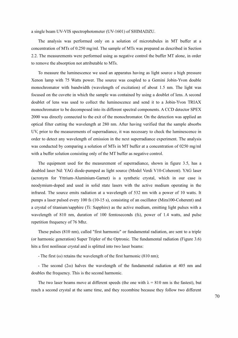
Many organic molecules absorb in the visible and UV spectra, but only few of them are
fluorescent (many of biological interest). Fluorescence is in fact influenced by the structure of
the molecule. Stiff molecules characterized by systems of conjugated double bonds such as
aromatic structures, are fluorescent. Of the twenty natural amino acids, only three have intrinsic
fluorescence: Tryptophan, Tyrosine, and Phenylalanine (Fig. 3.1). Each of these amino acids is
activated at a specific wavelength, but its luminescence is strongly influenced by the polarity of
the surroundings. This means that the maximum of the emission of these amino acids can
change: for example, a tryptophan excited between 270-280 nm, emits at 350 nm in water, while
well-protected inside a protein it emits at 330 nm. Since amino acids constitute the skeleton of
all proteins, many proteins are intrinsically fluorescent because of the presence of such aromatic
compounds.
The fluorescence emission spectra are different for the proteins that maintain the tertiary
structure compared to the same proteins that are denatured or unfolded. The phenomenon is so
influenced by experimental conditions: concentration, temperature, pH, phase of the sample,
way of supplying energy to the molecule, nature of the excited electronic state, pressure (in the
case of a molecule in the gas phase) and presence of other chemical species that can promote or
inhibit physical quenching and intermolecular energy transfer. Fluorescence quenching is a
process which decreases the intensity of the fluorescence emission. The accessibility of groups
on a protein molecule can be measured by use of quenchers to perturb fluorophores. Quenching
by small molecules either in the solvent or bound to the protein in close proximity to the
fluorophore can greatly decrease the quantum yield of a protein. Quenching may occur by
several mechanisms: collisional or dynamic quenching, static quenching, quencing by energy
transfer, charge transfer reactions [Morrison, 2008].
Temperature affects fluorescence because the vibration state of the molecule depends on
temperature, so it can contribute to the internal conversion. The fluorescence varies with the
variation of the solvent used: a non polar solvent ensures the emission of an extra quantum of
energy than a polar solvent.
The intrinsic fluorescence of tryptophan, tyrosine and phenylalanine (excited respectively at
295, 280 and 270 nm) is different depending on the more or less polar characteristics of protein
environment in which they are. They are also directly affected by the quenching effect, that is
the energy transfer to other structures, created by interactions with other aromatic molecules or
other chemical protein structures such as disulphide bridges, having the task of stabilizing the
tertiary structure. Therefore, the fluorescence emission spectra are different for the proteins that
maintain the tertiary structure compared to the same proteins denatured or unfolded. This
difference is both in terms of quantum yield of fluorescence and in terms of energy of the
61
emitted photon and of wavelength. The denaturation results in a lengthening of the shift of
Stokes of a few nm and a change of the intensity of the emission spectrum. Very often, the
fluorescence emitted increases because the quenching effects involving aromatic residues are
reduced. Other times the intensity of the fluorescence emitted is reduced during the process of
unfolding, because the protein in native form did not show quenching factors and the shift of
aromatic amino acids to a more polar environment reduces the quantum yield.
In the case of microtubules, the quantum yield (that is the ratio between absorbed and
emitted photons) increases in the chromophores that are not exposed to the polar solvent
(water). The peak of the emission can change. For example, a tryptophan, which is one of the
aminoacid constituent of tubulin, in water emits at 350 nm whereas a tryptophan well protected
in the protein emits at 330 nm. Within the microtubule cytoskeleton may occur quantum laser-
like coherent phenomena at long-range. The measurement of the fluorescence within
microtubules is introductory to the superradiant experiment.
The instrument used to measure the fluorescence is the spectrofluorometer. Its key
component is the light source that is usually a mercury lamp or a xenon arc that emits a
polychromatic radiation that is sent to a monochromator with continuous spectrum, M1, to
select the λ of the incident light beam [Lakowicz, 2002.]. The light is then sent to the cuvette
containing the sample, which once excited emits radiations at a λ greater than that of
excitement. This is sent to a second monochromator, M2, that select a specific λ of emission
(i.e., an incident radiation with fixed wavelength) thus determining the fluorescence spectrum of
the sample by sending it to a detection system (which is usually a highly sensitive photocell),
where a photomultiplier amplifies the signal that is finally registered. In a spectrophotometer,
the incident light I0, and the emitted light, I, follow the same direction. Instead, in a standard
spectrofluorimeter, the geometry changes, because this instrument allows light to penetrate the
sample through a portion on a face of the cell, and the emitted photon to exit at an angle of 90°
respect to the incident radiation (spectrofluorimeter at 90°).
62
Figure 3.1 Emission spectra of fluorescence on aromatic aminoacids in water
3.1.2 Resonance
Antennas are devices able to transform an electromagnetic field into an electrical signal, or
to radiate, in the form of electromagnetic field, the electrical signal they are fed by. When
powered by an electrical signal to their ends, antennas absorb energy and return it in the
surrounding space as electromagnetic waves (transmitting antenna), or absorb energy from an
electromagnetic wave and generate a voltage to their ends (receiving antenna). On theoretical
bases any conductive object acts as an antenna, regardless of the electromagnetic wave
frequency they are hit or the signal that is fed by. The magnitude of the effect becomes
significant when the frequency corresponds to the resonance frequency and in this case the
output voltage can be used for receiving and transmitting radio waves. The resonance is a
physical condition that occurs when a damped oscillating system is subjected to a periodic
solicitation with a frequency equal to the system oscillation. A resonance phenomenon causes a
significant increase in the extent of the oscillations that corresponds to a remarkable
accumulation of energy within the oscillator.
Recent observations and experiments on CNTs have led to the development of an array of
63
WAVELENGTH (nm)
PL
INTE
NSI
TY
Tryptophan
Phenylalanin
Tyrosin
WAVELENGTH (nm)
PL
INTE
NSI
TY
Tryptophan
Phenylalanin
Tyrosin
CNTs able to act as antennas [Wang et al., 2004]. Instead of transmitting and receiving radio
waves (measured in meters), these structures capture wavelengths at the nanoscale (measured in
nanometers) due to their small size.
In the study of the physical properties of MTs compared with those of CNTs, it is desired to
search and analyze a possible reaction to microwaves, observing any ability of MTs to absorb or
emit like antennas. Our experimental approach was intended to verify the existence of
resonance in MTs, in analogy with the CNTs, at the frequency that amplifies the wave.
The bench for the MTs resonance experiment consisted of a microwave generator with two
1⁄4 wave dipole custom antennas centered on a frequency of 1.5 Ghz (Fig.3.2). The antennas
have been placed on the same horizontal plane and spaced 4 cm. The test-tube containing the
solution was placed between the antennas. The system was placed in a Mu-metal container in
order to shield the measurement system from any external signal. The first antenna was
connected with a shielded cable to a Polarad mod. 1105 Microwave Signal Generator,
generating frequencies between 0.8 GHz and 2.5 GHz. The second antenna shielded cable was
connected with an Avantest mod. TR4131 Spectrum Analyzer. The experiment displays changes
in the resonance reference peak of the tested material. If the peak is lower the analyzed sample
is absorbing, if higher it is emitting electromagnetic energy.
We compared the responses of samples of MTs, tubulin and buffer solutions without
proteins when subjected to high frequency electromagnetic stimulations.
One ml of tubulin solution was placed in a plastic test tube positioned between the
transmitting and receiving antennas. In order to detect possible resonances on specific
frequencies, we carried out a frequency scan between 800 MHz and 2500 MHz using a
radiofrequencies generator and checking the presence of an absorption resonance, visible by
means of a difference in the peak amplitude, with an Avantest TR-3130 spectrum analyzer. The
same analysis was also performed on 1 ml of MTs solution and on 1 ml of Buffer MT.
64
Figure 3.2 Microwave Signal Generator.
3.1.3 Birefringence
Birefringence is an optical property of materials that arises from the interaction of light with
oriented molecular and structural components [Huang et al., 2005]. Birefringence is the
decomposition of a beam of light into two rays that occurs when the light crosses specific
anisotropic media depending on the polarization of the light. The interaction between light and
magnetic field in a medium results in the rotation of the plane of polarization proportional to the
intensity of the magnetic field component in the direction of the beam of light (Faraday effect).
The birefringence experiment was performed on solutions of tubulin and MTs, each in its
own stabilizing buffer. The final concentration for both tubulin and microtubules was 0.5
mg/ml. Then we repeated the tests with tubulin in MTs buffer and with the buffer alone as
control. The preparation of the buffers and the reconstitution of tubulin and microtubules are
described in section 2.2.
Each sample solution was submitted to four tests:
- Transverse electric field (1 volt/cm)
- Transverse magnetic field
- Longitudinal magnetic field
65
- No field
For each test the value displayed on the polarimeter directly measures the current in the
photodiode, expressing the intensity of the laser beam after passing through the cuvette. In
presence of a strong scattering, indicating a lack of organization in the sample, the intensity
decreases. To minimize spurious effects, the windows of the cuvettes are made of cover slip
glass about 18 microns thick. The spectrum analyzer window was set to see a width of 50 Hz,
within which range the frequencies of the two samples are included, the distilled water 610 Hz
reference and the analyzed 632 Hz solution.
We used two cells simultaneously; a first cell was always present with a low intensity
longitudinal magnetic field at 610.1Hz frequency and filled with distilled water. This allowed a
reference signal in all the various measures on the second cell, excited at a 632 Hz frequency.
The choice of almost static fields permitted the highest sensitivity. The frequency (632 Hz) is
sufficiently low to exclude dynamic effects. An important point is that for longitudinal magnetic
fields a strong Faraday Effect is present due to the water contained in the analyzed solution and
producing a consistent background noise.
For the measurement a polarimeter was prepared. In a classic polarimeter a monochromatic
source radiates a beam of light (initially not polarized) that is sent on a pair of polarized filters
(normally Nicol prisms) oriented so as to polarize light. The beam of polarized light crosses a
cuvette containing the test solution which, if optically active, rotates both polarization planes of
light. Finally, the beam passes through a polarized filter, the analyzer, whose main section is
rotatable. A more descriptive schema is depicted in figure 3.3.
B: cuvette and 610.1 Hz coil for the reference cell
C cuvette and 632 Hz coil for the sample
D: electric field cell
E: analyzer filter
F: lens that focuses the beam on the photodiode
G: photodiode and amplifier
HP: spectrum analyzer (HP 3582A) for on-line check
COMP: data acquisition system
The light source consists of a Hughes 3222HP Helium-Neon Laser, 633 nm, and power 5
mW. The magnetic field is 18 Gauss RMS for the 632 Hz test cuvette and 9.8 Gauss RMS for
the 610.1 Hz cuvette, while the applied electric field (632 Hz) is 1 Volt/cm RMS. The cuvettes
used for the magnetic field measured 15 mm, while that for the electric field was 23 mm long.
The transverse electric field was achieved with simple aluminium electrodes, 3 mm long and 5
mm high. The magnetic field (longitudinal or transverse) was obtained by a pair of Helmholtz
coils powered by sinusoidal generators. Electric field and transverse magnetic field were
oriented according to the horizontal and the first polarizer was oriented at 45 degrees with
respect to the direction of the transverse fields. The laser beam after the cuvette was examined
by a polarization analyzer oriented at 45 degrees with respect to the first polarizer and finally
sent to the photodiode: with this orientation the maximum signal is achievable by modulation
due to the Faraday Effect (longitudinal magnetic field). The photodiode was a HP 5082-4220
and the spectrum analyzer was an HP 3582A; the signal was sampled at 8000 samples/sec (Fig.
3.4).
67
Figure 3.4 Spectrum analyzer HP 3582A
The analysis of the signals was performed with Hamming windowing using home-made
analysis software written in FORTRAN at the Department of Physics (University of Milan).
Other tests have been performed using the Sigview® SignalLab software and have exploited
Hann and Hamming windowing, with or without Hann smoothing.
3.1.4 Superradiance
Superradiance phenomenon was first described by R. H. Dicke [Dicke, 1954], and consists
in the cooperative emission of an electro-magnetic radiation by a set of dipole coherently
coupled.
A single dipole oscillate at a frequency corresponding to the transition between two electric
states (S0 → S1); during oscillation a radiation is emitted, of intensity I proportional to the ratio
between the square of its charge q and its mass m: I ∝ q2/m. In a system made up of two dipoles
oscillating separatly, each one emits a radiation of intensity I = q2/m. Instead if the two dipoles
oscillate in phase, the radiation intensity emitted corresponds to that of an oscillating object with
charge 2q and mass 2m: I = (2q)2/2m → I = 2q2/m Therefore, in a system consisting of N
dipoles oscillating in phase, the total intensity of the radiation emitted is equal to: 68
I = (Nq)2/Nm → I = Nq2/m
From an experimental point of view, a radiation is sent to the sample to be analysed in order
to determine the excitation that is the transition form the fundamental state, S0, to the first
excited state, S1. Like all excited systems, it tends to return to the fundamental state S0, by
releasing energy.
This can happen through radiative decay, that is by emission of light; through inter-system
crossing, ISC, that is a decay on another excited state with different multiplicity; or through
non-radiative decay, that is via a return to the fundamental state without emission of photons,
and therefore with thermal dissipation of excess energy.
The expression [N(q2 /m)] indicates the speed of radiative decay of the system, but not its
intensity, that depends on the ratio of the speed of radiative decay as a function of the speed of
total decay. In order to demonstrate that the system is superradiant we should determine if there
are dipoles oscillating in phase, and if yes, how many they are. In a system of N molecules the
superradiance can be demonstrated experimentally by measuring the radiative lifetime of the
optical transition as a function of the number of the molecules where the excitation is
delocalized. This number theoretically overlaps the number of molecules of the system, but in
practice it is much lower because both static (defects, impurities) and dynamic (vibration)
disorder limit the length of delocalization of the excitement.
The efficiency of emission (Q.Y o Φ) is measured, corresponding to the ratio between the
number of photons emitted and the number of absorbed photons. Q.Y. depends on the number of
states decaying radiatively, with emission of a photon, and on the total number of states that
decay both radiatively and non-radiatively. Q.Y. is proportional to the luminescence intensity
experimentally observed (IPL). By measuring the lifetime of an emission and its intensity as a
function of temperature, it is possible to obtain the strength of the oscillator of the optical
transition, or in an equivalent way the radiative decay rate, which is inversely proportional to
temperature itself. This is the main proof that an emission is superradiant (necessary and
sufficient condition).
Since superradiance comes from the delocalization of the excitation, it has to be
accompanied by other effects. In particular, if excitation is delocalized over N molecules, the
square of the line width of a superradiant emission should be directly proportional to
temperature. This is a necessary but not enough condition for superradiance, since similar
effects may also be due to different phenomena.
The superradiance experiment requested in advance to verify the spectroscopic behaviour of
MTs, which is the study of their absorption in UV-VIS field. The measurement was made using
69
a single beam UV-VIS spectrophotometer (UV-1601) of SHIMADZU.
The analysis was performed only on a solution of microtubules in MT buffer at a
concentration of MTs of 0.250 mg/ml. The sample of MTs was prepared as described in Section
2.2. The measurements were performed using as negative control the buffer MT alone, in order
to remove the absorption not attributable to MTs.
To measure the luminescence we used an apparatus having as light source a high pressure
Xenon lamp with 75 Watts power. The source was coupled to a Gemini Jobin-Yvon double
monochromator with bandwidth (wavelength of excitation) of about 1.5 nm. The light was
focused on the cuvette in which the sample was contained by using a doublet of lens. A second
doublet of lens was used to collect the luminescence and send it to a Jobin-Yvon TRIAX
monochromator to be decomposed into its different spectral components. A CCD detector SPEX
2000 was directly connected to the exit of the monochromator. On the detection was applied an
optical filter cutting the wavelength at 280 nm. After having verified that the sample absorbs
UV, prior to the measurements of superradiance, it was necessary to check the luminescence in
order to detect any wavelength of emission in the next superradiance experiment. The analysis
was conducted by comparing a solution of MTs in MT buffer at a concentration of 0250 mg/ml
with a buffer solution consisting only of the MT buffer as negative control.
The equipment used for the measurement of superradiance, shown in figure 3.5, has a
doubled laser Nd: YAG diode-pumped as light source (Model Verdi V10-Coherent). YAG laser
(acronym for Yttrium-Aluminium-Garnet) is a synthetic crystal, which in our case is
neodymium-doped and used in solid state lasers with the active medium operating in the
infrared. The source emits radiation at a wavelength of 532 nm with a power of 10 watts. It
pumps a laser pulsed every 100 fs (10-15 s), consisting of an oscillator (Mira100-Coherent) and
a crystal of titanium/sapphire (Ti: Sapphire) as the active medium, emitting light pulses with a
wavelength of 810 nm, duration of 100 femtoseconds (fs), power of 1.4 watts, and pulse
repetition frequency of 76 Mhz.
These pulses (810 nm), called "first harmonic" or fundamental radiation, are sent to a triple
(or harmonic generation) Super Tripler of the Optronic. The fundamental radiation (Figure 3.6)
hits a first nonlinear crystal and is splitted into two laser beams:
- The first (ω) retains the wavelength of the first harmonic (810 nm);
- The second (2ω) halves the wavelength of the fundamental radiation at 405 nm and
doubles the frequency. This is the second harmonic.
The two laser beams move at different speeds (the one with λ = 810 nm is the fastest), but
reach a second crystal at the same time, and they recombine because they follow two different70
paths through a system of mirrors.
From this second crystal 3 different lasers are drawn:
- Fundamental radiation, ω (λ = 810 nm);
- Second harmonic 2ω (λ = 405 nm);
- The third harmonic, TGH, which triples the fundamental frequency of the radiation and
divides it by 3, at 270 nm.
The third harmonic is focused with a spherical mirror on the sample, where packets of
photons arrive at a frequency of 76 MHz spaced from one another by 14 ns and 150 fs wide.
The sample absorbs light and luminescence just a result of this pulsed excitation.
The luminescence is collected by a lens system and sent to the entrance slit of a
spectrograph from Chromex, namely a polychromator with a bandwidth of about 5 nm, coupled
with a Streak Camera (SC) from Hamamatsu. When the light reaches the lattice, it is split in the
plan in its different spectral components and is sent to the SC.
The SC is an electronic device capable of analyzing the temporal evolution of
electromagnetic radiation on scales up to a few picoseconds (Figure 3.7). Schematically it
consists of a photocathode of cesium iodide (CsI), a 50/40 intensifier and a camera with
appropriate focusing optics that amplify and collect the light coming from a screen of
phosphors. The photocathode, which is the element of the SC sensitive to visible radiation,
converts photons into electrons on the sensitive plate of CsI via the photoelectric effect. The
electrons are then accelerated by a strong electric field, they enter between two parallel plates of
a capacitor and all get through it with the same time length. Inside the capacitor a “saw tooth”
voltage is applied, which serves to split the different electrons: electrons arriving before are
affected by a low electric field and are deflected less than the electrons that arrive later and are
more deflected. The information time (Δt) is thus encoded in terms of spatial coordinates (Δx).
A signal extended in time is converted into a strip of electrons on the detector. A magnetic lens
focuses the emitted electrons. The split electrons impact on a phosphor screen that reconverts
them into photons. The photons, in turn, impress a CCD (Charge-Coupled Device) which
“photographs” the phosphor screen. Finally, the software package converts the position of
several photons on the CCD in a graph showing the wavelength on the abscissa and time in
ordinate. The SC has a temporal resolution of up to 2 ps; in our case, however, it has been used
with a lower resolution (30 ps) because the time of luminescence of MTs was much longer.
The analysis was conducted on a solution of MTs in MT buffer at a concentration of 0.250
mg/ml. The sample was placed inside the cryostat apparatus and frozen in an atmosphere of
71
inert gas (N2 gas) up to a temperature of 80 Kelvin. At this temperature a first acquisition was
performed by exciting the sample with a radiation at λ of 270 nm and measuring the lifetime of
the luminescence emitted. Then gradually increasing the temperature up to the melting
temperature of the sample other acquisitions were performed, measuring at each time the
lifetime of the emitted signal.
Figure 3.5 Equipment used for the measurement of superradiance
Figure 3.6 System for tripling a laser pulse
72
Figura 3.7 Scheme for the functioning of the Streak Camera
3.2 COMPUTATIONAL AD HOC METHODS
In order to analyse the experimental results and draw conclusions on the issue of abnormal
biophysical properties of microtubules computational methods were used in synergy:
- Physico-Chemical Simulation Environment
- Dynamic Simulation Environment
- Self-organizing Artificial Neural Networks for the study of the evolution of the dynamic
organization of microtubules and tubulin under the influence of electromagnetic fields
- Analysis of the outputs of neural networks through the method of conflict and occupation and
the method of attractors
3.2.1 Molecular Dynamics
The molecular models of the elements used for the simulation were obtained through the
online consultation of two databases: Research Collaboratory for Structural Bioinformatics,
RCSB, which is in charge of the archiving and document digitization of 3D molecular structures
obtained by X-ray crystallography and spectroscopy, and PubChem, a database of chemical
molecules, maintained and funded by the National Center for Biotechnology Information. The
PubChem database is access free, and millions of compounds structures and descriptive data can
be downloaded via FTP. PubChem contains descriptions of molecules with less than 1000 atoms
and 1000 bonds. X-ray crystallography is the main method for determining molecular
conformations of biological macromolecules, in particular of proteins and nuclei acids such as
DNA and RNA. The format obtained from the consultation of the RCSB is called Protein Data
73
Bank (PDB) [Berman et al., 2007]. It is a text file describing the three-dimensional structure of
all the molecules of the system. Most of the information contained in the database is related to
proteins and for this reason the intramolecular bonds are rich in descriptive properties.
Typically, a file of this type is defined by a set of information:
- ATOM field: describing the coordinates of the atoms constituting the proteins. For
example, the first line is the first atom compound, the first three floating point numbers are the
coordinates X, Y, Z expressed in Angstrom (unit of measurement that indicates the length of
chemical bonds) [Protein Data Bank Atomic, PDB, Coordinate Entry Format Version 3.2. ]. The
next three columns show respectively the occupation, the temperature factor and the name of the
element.
- HETATM field: describes the coordinates of the hetero-atoms, ie atoms that are not part of
the protein molecule.
- SEQRES field: giving the sequence of peptide chains.
- REMARK field: this is a comment field containing information in free form. It is usually
referred to research papers that led to the creation of the model but also to the sequence of the
coordinates of the calculation useful to create the model.
- HEADER, TITLE and AUTHOR field: showing the name of the researchers who defined
the structure.
Through the years, the file format has undergone many changes and revisions. Its original
size was dictated by the width of the device for the punch cards (80 columns) previously used
for the upload of models. A XML version of this format, called PDBML, was described in 2005
[Westbrook et al., 2005].
The PDB files have as identifier a file name consisting of alphanumeric characters (i.e.
1TUB or tubulin). Each published structure is then identified through its PDB ID, but this can
not be used as an identifier for biomolecules, because often there are different structures for the
same molecule (in different environments or conformations). Figure 3.8 shows the PDB file for
tubulin.
The molecular models archived in the database are presented in the format PubChem SDF
(Structure Data File). It organizes the molecule through biophysical features separated by a
separator. The first line of the file contains a unique identifier of the item. This number is
closely related to the structure and is the definition and the search key in the database. The
bonds are described by indicating the position in three dimensional space and charges through
the numerical data in the field partial charges.
74
By using this archive of molecules the models of microtubule and tubulin were obtained. To
verify that these models did meet the specifications recreated in the laboratory, Ascalaph
Designer was used [http://www.agilemolecule.com/Ascalaph/Ascalaph_Designer.html.
BlueTractorSoftware. Agile Molecule], a software that allows to build and simulate molecular
models and turn them into a three-dimensional environment. It also provides a graphical
environment for classical and quantum modelling of molecules based on Firefly [Gordon and
Schmidt, 2005] and MDynaMix/MGE [Lyubartsev and Laaksonen, 2000]. Both graphical
environments on which the simulator is based provide dedicated implementations for the
interaction of a large number of atoms, even if they can not reach, for obvious reasons, the
computational power that they can have with implementations based on cluster systems
[Lyubartsev and Laaksonen, 1998] or with dedicated hardware Molecular Dynamics-NVIDIA
Corporation.
In order to link together the various software used, it was necessary to use a format
converter, such as Avogadro. Avogadro is an open source platform recently created as part of the
project Open Molecules. Avogadro allows us to deal with simple and complex molecules with a
high speed and good usefriendliness. The molecules can be represented in different ways, such
as balls and sticks, orbitals, Van der Waals spheres, surfaces, rings and hydrogen bonds. A wide
range of fragments are available immediately in a drop down menu with the ability to choose
the single, double and triple bonds. The molecules created can be manipulated, inter-atomic
distances can be viewed, bond angles can be oriented. The molecules created can be handled in
several formats, including the most popular such as PDB, MDB, Gaussian, and can be exported
in a graphical format JPG, BMP and PNG. Regarding the upload, the program is based on Open
Babel and is able to read and convert over 80 formats.
75
HEADER MICROTUBULES 23� SEP� 97 1TUB
TITLE TUBULIN ALPHA�BETA DIMER, ELECTRON DIFFRACTION. . .KEYWDS MICROTUBULES, ALPHA�TUBULIN, BETA�TUBULIN, GTPASEEXPDTA ELECTRON DIFFRACTIONAUTHOR E.NOGALES,K.H.DOWNING. . .JRNL AUTH E.NOGALES, S .G.WOLF,K.H.DOWNINGJRNL TITL STRUCTURE OF THE ALPHA BETA TUBULIN DIMER BYJRNL TITL 2 ELECTRON CRYSTALLOGRAPHY.JRNL REF NATURE V. 391 199 1998JRNL REFN ASTM NATUAS UK ISSN 0028�0836REMARK 1REMARK 1 REFERENCE 1REMARK 1 AUTH E.NOGALES, S .G.WOLF,K.H.DOWNINGREMARK 1 TITL ERRATUM. STRUCTURE OF THE ALPHA BETA TUBULIN DIMERREMARK 1 TITL 2 BY ELECTRON CRYSTALLOGRAPHYREMARK 1 REF NATURE V. 393 191 1998. . .REMARK 500 ATM1 RES C SSEQI ATM2 RES C SSEQIREMARK 500 CD GLU B 71 CB ALA B 99 0.41REMARK 500 OG SER A 170 SD MET A 203 0.54REMARK 500 CB SER A 165 OD2 ASP A 199 0.88REMARK 500 CG PRO B 184 CD2 PHE B 399 0.91REMARK 500 O VAL A 363 OD2 ASP A 367 0.94REMARK 500 NH1 ARG A 2 OD2 ASP A 251 1.01REMARK 500 O MET A 154 NE2 HIS A 197 1.04REMARK 500 OD2 ASP A 205 CG1 VAL A 303 1.04. . .SEQRES 1 A 440 MET ARG GLU CYS ILE SER ILE HIS VAL GLY GLN ALA GLYSEQRES 2 A 440 VAL GLN ILE GLY ASN ALA CYS TRP GLU LEU TYR CYS LEUSEQRES 3 A 440 GLU HIS GLY ILE GLN PRO ASP GLY GLN MET PRO SER ASPSEQRES 4 A 440 LYS THR ILE GLY GLY GLY ASP ASP SER PHE ASN THR PHESEQRES 5 A 440 PHE SER GLU THR GLY ALA GLY LYS HIS VAL PRO ARG ALASEQRES 6 A 440 VAL PHE VAL ASP LEU GLU PRO THR VAL ILE ASP GLU VAL. . .ATOM 1 N MET A 1 �26.006 52.343 �25.121 1.00 20.00NATOM 2 CA MET A 1 �25.759 52.677 �23.728 1.00 20.00CATOM 3 C MET A 1 �26.559 53.689 �24.177 1.00 20.00CATOM 4 O MET A 1 �26.668 54.651 �23.359 1.00 20.00OATOM 5 CB MET A 1 �24.344 52.329 �23.334 1.00 20.00CATOM 6 CG MET A 1 �24.068 50.890 �23.389 1.00 20.00C. . .HETATM 6792 PG GTP A 500 �57.551 49.025 �35.493 1.00 20.00PHETATM 6793 O1G GTP A 500 �56.753 49.937 �34.642 1.00 20.00OHETATM 6794 O2G GTP A 500 �57.704 49.788 �36.825 1.00 20.00O. . .
Figure 3.8 PDB file for tubulin (1TUB.pdb). Only the first rows are shown.
76
3.2.2 Dynamic System Evolution
The theoretical assumptions of the computational methods used in this thesis are based on
the theory of dynamic evolution of complex systems and on the properties originating from their
self-organization capacity. Both tubulin and MTs behave as complex systems and we are able to
examine their dynmic evolution by means of suitable computational mehods.
The theory of complex systems deals with the study of the organization spontaneouslyemerging from the interaction of many elementary components [Heylighen 1992; Gell-Mann,1995]. Complex systems respond to changes in the external environment reorganizingthemselves in order to exhibit novel properties [Standish, 2002].
The self-organization is a space-time structure that is not imposed from outside but
spontaneously emerges from the evolution of the system as a function of its dynamics. The
emerging organization can be observed at a different and much higher time-space scale than the
molecular one. The construction of mathematical models for such systems [Rosen, 1972] shows
that the equations that govern them are generally very sensitive to initial conditions, so that
extremely small fluctuations give rise to completely different dynamic stories. This is called
"deterministic chaos": the system has an overall regular behaviour, which is irregular in detail,
and so it is impossible to predict its behaviour in the next instants.
Chaos can be defined as an unpredictable behaviour of a deterministic dynamical system
due to its sensitivity to initial conditions. The behavior of a dynamical deterministic system ispredictable once the initial conditions are known. But there are cases when the motion of thesystem has very different behaviours, according to the precision with which the initialconditions are measured. More specifically, a set S exhibits sensitivity to initial values if there is
a ρ so that for any ε > 0 and for any x in S, there is a y so that |x - y| <ε, and |xn – yn | > ρ forsome n> 0. Then there exists a fixed distance r so that there are nearby states that in the endmove away to a distance r, even if the initial state has been exactly defined. This is whathappens in chaotic systems. A chaotic system exhibits sensitivity to initial conditions behavingas a complex system.
A typical example of self-organization and is present in all biological systems [Green, 1994]
and in their most advanced expression, that is intelligent life. A promising attempt to reproduce
advanced features through the collective behaviour of simple elements is represented by the
artificial neural networks. Several interconnected elements continually exchange information on
the basis of a range of input from outside, and reach a form of functional organization that is not
caused by a default algorithm defined from the outside, but emerges from the same structure as
the neural system.
77
In the traditional approach complex systems are treated analytically, namely reducing them
to the linear combination simple elements. In nature many systems are linear or approximable to
linearity (i.e. electromagnetic waves: every periodic mathematical function can be represented
as a series of pure sigmoids by the Fourier transform). This has enabled the modelling of many
natural phenomena. But for many physical systems the linearity is not sustainable, and their
modelling becomes very complex: nearly all dynamic systems are chaotic, that doesn't mean
they are inherently indeterministic, but that they are not predictable [Kaplan and Glass, 1995;
Jackson, 1989]. The development of strictly time-varying and nonlinear spatial-temporal
pattern, such as those from the acquisition of experimental data, is an issue of increasing
importance, and its complexity has to involve the use and the development advanced tools. Thetypical adaptivity of artificial neural networks and their ability of generalization make them a
tool of choice for the analysis of this issue. No real model is truly linear, but often a linear
function can be approximated. The non-linear systems exhibit complex effects that are not
inferable with linear methods. This is particularly evident in dynamic systems [Atmanspacher
and Kurths, 1992].
A dynamic system is a system that expresses the variability of a state over time (ie a point in
a vector space). dX/dt = F(X,t) (1)
F: W Rn Rn differentiable
The solution of the system is the set of trajectories as a function of initial conditions. A dynamic
system is completely defined by a space of phases or states, whose coordinates describe the
system at all times, and by a rule that specifies the future development of all the variables of the
state.
Dynamical systems can be defined as deterministic if there is only one result for each state,
stochastic if there is more than one consequent with a certain probability distribution. The phase
space is the collection of all possible states of a dynamic system. It can be finite or infinite. If
some trajectories converge at some point, the set of initial states of these trajectories generated
is called region of attraction of the point. A region of attraction is a set of points in the state
space of finite diameter such that every trajectory enters and doesn't come out any more.Mathematically, a dynamic system is described by an initial value problem. The trajectory in thephase space traced out by a solution of an initial value problem is call the trajectory of thedynamic system.
We define as constant trajectory a constant solution x (t) = x (0) of (1), i.e. a vector x (0) sothat each component of the right side of (1) is zero. A constant trajectory is considered stable ifthe following conditions are satisfied:
78
- there must exist a positive number ε such that any trajectory that starts within ε of x (0)should asymptotically get close to x (0)
- for every positive number ε there must be a positive number δ ε ) such that a trajectory
that is initiated within δ ε ) remains within ε of x (0)
The set of all points which may have initial trajectories that asymptotically approach to astable trajectory is called region of attraction of the stable trajectory. A limit cycle, or cyclicattractor, is a closed curve in the n-dimensional space characterised by the following properties:
- no consistent trajectory is contained in the limit cycle
- any trajectory that begins at a point in the limit cycle should stay within the limit cycle
- there must be a positive number ε such that each trajectory of the cycle that starts within ε
should asymptotically approach the limit cycle
- for every positive number ε there must be a positive number δ ε such that a trajectory
that is initiated within δ ε of the limit cycle stays within the limit cycle
In summary, if some trajectories converge at some point, the set of initial states of these
trajectories is called region of attraction of the point. A region of attraction is defined as a set of
points in the state space of finite diameter such that every trajectory enters and doesn't exit. A
very common type of self-organization established in nature is the deterministic chaos. The
long-term behaviour of chaotic systems follows organised pattern detectable by viewing the
trajectory of the system in the state space. These trajectories show a spatial structure in which
they are confined in an odd attractor, which is exhibit some regularity, but are not strictly
recurrent [Peitgen et al. 1992]. An odd attractor is geometrically a fractal [Mandelbrot, 1983],
that is a structure with a not entire size.
A neural network can be considered as a dynamic system of n-dimensional differential
equations describing the dynamics of n neurons. Each neuron is mathematically defined by its
state x(i) and by its gain function gi=gi(xi) differentiable everywhere and not decreasing. A
typical gain function is for example the logistic function
g(x) = (1 + e -x)-1
biologically motivated because it simulates the refractory phase of real neurons. This function
returns values between 0 and 1. It is often useful, however, the use of a transfer function
symmetric respect to zero, in order to maintain the symmetry of input values. It is then used the
hyperbolic tangent function (between -1 and +1), or the functionF(P) = A (ekp –1) / (ekp +1)
where A and k are positive constant. The variation speed of each xi is determined by a function depending on xi and on the output
79
gi(xi). In general, such variation can be expressed with the system of differential equations dxi/dt = -ki xi + pi (g(x)) (2)
where ki is a positive constant and each pi is a polynomial function of the n variables g1(x(t),
g2(x(t),..., gn(x(t)), that behave well enough to ensure that the trajectories for the system of
equations exist and are unique.
The purpose of the neural network is to generate trajectories in n-dimensional space
approaching asymptotically some of the attractor trajectories. Activity levels of n neurons are
represented by a point in n-dimensional space [Jeffries, 1991]. A n-dimensional dynamical
system is therefore built and its solutions are trajectories representing constant attractors (stable
equilibrium) or cyclic attractors (limit cycles). The Hopfield network is a prominent example of
how a neural network is a dynamic system that can tend to a number of stable attractors.In additive neural models, such as MLP, each pi is a linear function of the component of g:
pi = Σnj Tij gi (3)
where Tij are real constants forming a matrix nxn.
Recently, however, alternative more efficient neural networks of higher order have emergedin which each pi is a polynomial function of the components of g, typically of the form
g1e1g2
e2...gn en where each exponent ei is equal to 0 or 1.
For linear networks of the type (3) the theorem of Cohen-Grossberg [Hecht-Nielsen, l990]
ensures the existence of stablepoints (i.e. points for which dx(p)/dt = 0).
According to the theorem of Cohen-Grossberg, each dynamic system with the form
dxi/dt = ai(xi) [bi(xi) - Σj wij Sj (xj )]
such that1) the matrix wij is symmetrical and every wij >=0
2) the function aj (x) is continuos if x>=0 and aj (x)>0 if x>0
3) the function bj (x) is continuos and finite for every open interval when x>0
4) the function Sij (x) is differentiable and S’ij (x)>0 if x>=0
5) bj(x) – wiSi(x)<0 if x-->
6) lim u-->0+ bi(x) < and ∫ 1/a(s) ds = for some x>0
has at least a countable set of stable points p such that dx (p)/dt = 0.
If the network status at time 0 is such that xi(0)>0, then the network will almost alwaysconverge at some stable point p (such that dx(p)/dt=0), and there will be at least one countable
set of such points. Even if such conditions are restrictive, they match with those supported by
many self-associating networks (i.e. the Hopfield network, with fully interconnected nodes and
symmetrical weights). The memories are placed in the attractors, and the theorem guaranteestheir existence, in spite of the existence of many spurious attractors.
80
Each state of a network can be associated with a Lyapounov energy function that helpsdetermining certain properties of the trajectories. A Lyapounov function (L) is a function:
L : {0,1} n ---> R such that
L(T(x)) L(x) for each x {0,1}n
where T is the function of the transition made by the network. Therefore L is a monotone non-increasing function along each trajectory. There follows that the equilibrium points of the
system correspond to the points of minimum of L. For networks with square connection matrix,
the function L is called energy function and is chosen as
E(x) = -1/2 ΣiΣxj wij xj xj
clearly indicating that it is monotone non-increasing and that ∆E is always <=0 (i.e. the systemis overall stable).The Hopfield network is a prominent example of how a neural network is a dynamic system thatcan tend to a number of stable attractors. It is a fully connected network with symmetricweights, bipolar input (+/-1 or 0,1). The inputs are simultaneously applied to all nodes and theweights are set according to the law
wij = Σ xii xj if i< >j
wij = 0 if i=j In the learning cycle each output of a neuron is a new input for the same neuron. The calculationof the new value is determined by the function:
f(xi )= xi se Σwij xj = Ti (possibly null threshold)
f(xi ) = +1 se Σwij xj > Ti
f(xi ) = -1 se Σwiij xj < Ti
A pattern of input can be seen as a point in the space of states, that while the network iterates it
moves towards the valleys, representing the stable states of the network. The ultimate values of
the weights represent the output of the network. The solution comes out when the point moves
in the lowest region of the basin of attraction. In fact, for symmetric matrices with null diagonal
ΔE/Δxi = - Σwij xj
if Δxi >0, that Σwij xj >0
if Δxi <0, then Σwij xj <0
that is always ΔE <=0.
After a certain number of iterations the network stabilizes in a state of minimum energy.
Each minimum correspond to a pattern stored in the network. An unknown pattern is a point on
this hyper plane, which gradually moves towards a minimum point. There may be so-called
meta-stable states, i.e. minimum points which do not match any stored pattern (spurious
attractors).
81
More generally the following theorem (4) can be demonstrated: each neural network model
of type (2) has a finite region of attraction (Fig. 3.9).
Figure 3.9 Typical trajectories in two-dimensional space with two memories and limit cycle model.
Once a particular dynamic model and its attractors have been identified, a learning
algorithm varying the locations of the fixed points to encode information needs to be
established. A sufficient condition for the existence of this algorithm is therefore the existence in
the system of stable isolated attractors, i.e. fixed points. The matrix of weights will be adjusted
so that, given an initial state x0=x(t0)), a given input corresponds to a fixed point x∞ = x(t∞),
whose components have a desired set of values Dj in the units of the output. A typical method
used in back-propagation networks, is to minimize a function E measuring the distance between
the desired fixed point (attractor) and the current fixed point:
E = 1⁄2(Σi Ji ) where Ji = (Di – xi ∞ ) Qi
Qi is a function that is 1 or 0 depending on whether the i-th unit belongs to the subset of theoutput of the network units or not. Then the learning algorithm moves the fixed points so as tosatisfy on the output units the equation
x(t∞) = Di
A typical way to do this is to make the system evolve in the space of the weights along thetrajectories that are antiparallel to the gradient of E:
τ dwij/dt = - dE/dwij
where τ is a numerical constant defining the time scale for the changing of w; τ should be low,so that x is always at a steady state, i.e. x (t) = x ∞.
When on the output layer the error between the desired and the actual output is calculated,this error is propagated backwards in the various layers, in order to adjust the weights of eachnode. This algorithm, called the decreasing gradient and used by back-propagation networks[Rumelhart et al., 1986], is not the only possible one but is without doubt the most efficient and
simple equation minimizing E. If the initial network is stable, the dynamics of the decreasing
82
gradient does not change the stability of the network. This allows us to state the reliability of the
back-propagation algorithm, which provides the necessary robustness to the deviations
produced by interference and present in real systems.
An example of self-organizing dynamic system is represented by the unsupervised neural
networks [Carpenter et al., 1991; Cohenet et al., 1987] as the Self-Organizing Map (SOM) of T.
Kohonen. The structure of a Kohonen network consists of a layer of N elements, called
competitive layer. Each layer receives n signals x1, ..., xn coming from an input layer of n
elements, whose connections have weight wij. If the competitive layer is matrix-type, neurons
are interconnected in a square, hexagonal or rhomboidal scheme. If it is a vector-type, the
neurons are simply connected together to form a chain (Fig. 3.10).
Figure 3.10 Kohonen network.
To estimate the intensity Ii of the input of each element of Kohonen layer the procedure isthe following:Ii = D(wi,x)
wi=(wi1,...,win)T
xi =(xi,...,xn)T
where D (w, x) is a distance function, such as the Euclidean one. At this point a competition isperformed to identify the element with the lowest input intensity (that is which w is the closestto x).
The SOM provides a procedure known as lateral inhibition that is present also in nature in
the form of chemical changes at the synaptic level (fig. 3.11). In the cortical region of the brain,
in fact, neurons in close physical proximity to an active neuron show stronger links, while at
some distance from the active neuron start to show inhibitory connections. In this architecture,
each element receives both excitatory stimuli by adjacent elements (the so-called
neighbourhood), and inhibitory stimuli by farther neurons. The existence of the neighbourhood
is useful because it doesn't let the network to polarize on a few winning neurons.
83
Figure 3.11 Lateral Inhibition
In this way only the elements with a distance below a certain level are activated, and in
restrictive cases only the unit with minimal distance.
The learning process occurs in the so-called “Winner Take All Law” (WTA); the training
data consist of a sequence of input vectors x. Kohonen layer then decides the winner neuron
based on the minimum distance. The SOM performs a vector quantization that is a mapping
from a space of many dimensions in a space with fewer dimensions, while preserving the initial
topology. In other words a form of Nearest Neighbour (NN) clustering is performed, in which
each element of the competitive layer represents the membership class of the input elements.
The NN classification classifies a pattern according to the minimum value obtained among
all the distances from a set of reference pattern. This method is useful for separating classes that
can be represented by segments of hyper planes. For this reason, the SOM is useful to classify
patterns topologically well-distributed, but it is not good at classifying non-linear distributions.
There are however several reasons that limit the performance of the SOM in the case of non-
linear and time-varying input. First, the competitive layer is not able to unravel on the shape of
the topology if the non-linearity of the input topology is too accentuated. The second reason is
the difficulty of reaching a certain convergence, in the absence of the possibility of establishing
an error for each epoch of the network. The third reason is the low cardinality of the output,
limited to the number of the neurons of the competitive layer. Another problem of the SOM,
which is typical of any clustering algorithm, is the lack of explanation the output. Once the
classification of the input has been obtained, the user has to extrapolate the meaning with an adhoc procedure, which in real-time applications can further penalize the computational load. One
solution successfully tested was found following the analysis of time series of winning neurons
to changing times. That series tends to organize into a chaotic attractor that keeps stable as
epochs increase and whose characteristics uniquely identify the input pattern that created it (Fig
84
3.12).
Figure 3.12 Series of winning neurons in 2D state space; x-axis: from 0 to 20 (order number of the weight); y-axis: from -5 to +5 (value of the weight)
Based on this evidence the ITSOM (Inductive Tracing Self-Organizing Map) has been
developed. The time line of the winning neurons in a SOM tends to repeat itself, creating a time
series constituting chaotic attractors or precise limit cycles that uniquely characterize the input
element that produced them (Figure 3.13).
In fact, because of the learning rule, the winning weight represents an approximation of the
input value. At any epoch, the new winning weight along with the weight that has won the
previous epoch, form a second order approximation of the input value. It is therefore possible to
derive the value of the input by comparing the characteristic configurations of each input with a
set of reference configurations, whose value is known. A real process of induction is thus made,
since once a vector quantization many-to-few is produced from the input onto the weights layer,
a step few-to-many is performed from the reference configuration to the whole of the inputs.
85
Figure 3.13 ITSOM architecture
This form of induction is much more subtle than the one derived from the sole winning
neuron of a SOM network led to convergence to the corresponding input, because the neurons
of the competitive layer are too few to provide a significant classification.
The characteristic of this network is that it does not need to be brought to convergence,
because configurations of the winning neurons achieve the necessary stability within about tens
epochs. For best results the network shouldn't polarize on too few neurons, but shouldn't even
disperse itself throughout the whole layer.
The algorithm that resulted optimal to recognize the configurations created by the network
is based on the method of z-score.
The cumulative scores for each input are normalized according to the distribution of thestandardized variable z given by
z= (x – μ ) / σ
where μ is the average of the scores on the neurons of the weights layer and σ is the standarddeviation.
Once a threshold 0 < τ <= 1 is set, which is therefore one of the parameters of this network,these values are then set:
z= 1 per z > τ
z= 0 per z <= τ.
In this way, each configuration of winning neurons is represented by a binary number
composed of strings of 1 and 0, as many as are the weights of the output layer. It is then
straight-forward to compare these binary numbers.
Other methods are possible for discriminating winning configurations, always taking into
account that the fuzzyfication of their numerical strength is necessary, as they describe chaotic
86
attractors consisting of a repetitive nucleus with many variations in their surroundings.
The lateral inhibition mechanism of the SOM was written taking into account the
mechanisms of neurophysiological mapping of sensory stimuli on the neocortex: therefore,
similar inputs are mapped to nearby locations of the cortex in an orderly and conservative
topology.
Both in the SOM and in the other artificial neural networks the learning process is based on
cyclical repeating of input stimulus. Even in the brain there is evidence of reverberating circuits
that reinforce the impression of the input information on the cortical map. However, it appears
unlikely that these loops can be repeated thousands of times in search of a fixed target, also
because it is difficult to imagine that the brain can then recognize only the last active neurons as
the most important. It seems rather more reasonable to assume that reverberation naturally gets
exhausted with the unwinding of the electrical discharge activation, and that the cortical maps
are formed by a constellation of active neurons, the so-called memory trace, which will
subsequently retrieve information. For this reason, the ITSOM mechanism seems more
physiologically justified. Also the inductive mechanism, learning a very large number of new
information using the primer track of a nucleus of existing information, seems reasonable and
confirmed by neurophysiological experiments. Both daily experience and several studies seem
to confirm that learning is neither a fully supervised (i.e. based on examples), nor a completely
unsupervised process, and therefore it needs at least one set of known reference points.
SOM can also be expressed as a nonlinear dynamic model expressed by differential
equations dxi/dt = Ii – µ (xi), where the output variable xi can correspond to the average
frequency of discharge of the neuron i, Ii is the combined effect of all inputs on the neuron i, and
µ(xi) is the sum of all the non-linear losses encountered by discharge [Ritter and Schulten,
1988].The SOM architecture has been studied by Kohonen as a result of his studies ofneurophysiology [Kohonen, 1993], and .other authors observed the WTA functionality at thecortical level. Ermentrout [Ermentrout, 1992] studied a model of the cortex in which the WTAprocess has the dual role of selecting the more important stimulus and reinforcing the patternafter the stimulus has disappeared. Every time a cell is active for some time and then turns off,the network oscillates between different states. The occurring limit cycles are the result of thebifurcation solutions of the system
dxj/dt = -μxj + F(xj, u(t); α) j = 1,..., N
for N activated neurons xj, where F (x, y; α) is a function of two variables parameterized by αand such that F/dx>0 and F/dy<0, u (t) is the inhibitory feedback of the form
u(t)=G (Σxk),
87
G is monotonically increasing. The overall activity x1(t) + ... .+ xj(t) almost lie on a closedtrajectory, which means that the total excitatory activity of the network remains almost constant.Also Traub [Traub et al., 1991] introduces a biophysical model of this effect in which, even ifthe individual neurons randomly discharge, the entire system has a regular behaviour,constituting "limit cycles that preserve order".
In order to evaluate the results of the dynamical simulations, we conceived a novel method
based on Artificial Neural Networks (ANNs), which are effective non-linear classifiers, useful
for complex patterns. We submitted the structural data obtained by the MD evolution to two
different SOM-based models: SONNIA, a SOM-based algorithm developed in the SONNIA
environment, for the evaluation of specific parameters, and ITSOM for the evaluation of
dynamic attractors. Their results were then compared. Values of xyz coordinates of the
molecules after dynamic simulation and with minimized energy are used as input value for
neural networks.
For our case study we chose a Kohonen rectangular network structure with 9x6 neurons and
a random initialization. This map represents the number of neurons affected by the evolution of
the network and the values involved.
The first adopted model was a SOM-based algorithm developed in the SONNIAenvironment. SONNIA is a powerful Artificial Neural Networks environment, very useful in
the field of drug discovery and protein prediction. It allows classifying a series of data sets,
providing both supervised and unsupervised learning.
In this research project we have instead decided to use the analysis tools provided by
SONNIA to develop a SOM network and evaluate specific parameters to assess the degree of
dynamic organization reached by the examined molecules when subjected to electromagnetic
fields.
The output maps of a SOM network are represented in SONNIA by a set of coloured boxes,
one for each output neuron. The boxes configuration highlights two interesting parameters:
1 - Occupancy, i.e. the number of patterns that have been mapped onto the same neuron,
indicating similarities in the input domain.
2 - Conflicts or conflict neurons, i.e. neurons that refer to inputs belonging to different
classes.
In general, there are always at least a few conflicts such as with any other modelling
technique there are false positives or false negatives. 88
The main features that make the SOM-based algorithm developed in the SONNIA
environment SONNIA environment a useful tool for our analysis are: the processing of data
from projects of high dimension of space in two dimensions, the procedures for classification
and clustering, the modelling and prediction of structures, the planar or toroidal selection of the
topology of the network, the visualization of data as chemical structures, reactions and spectra.
Through the graphical interface of the SONNIA environment it is possible to upload the
appropriate data file, and a neural network can be created by defining the parameters of its
architecture: the algorithm to be used, the topology of the network, the dimension of the
neurons, the dimension of the network and the initialization process. Once the definition of the
parameters is completed, the neural network can be trained. The first phase of the training
activates the learning speed, the length of learning, the error checking and the threshold arrest,
and the values for the epochs and for the intervals to be set.
After the training has been completed it is possible to start working with the network. The
SOM-based algorithm developed in the SONNIA environment permits to visualize the changing
of dynamic errors during training and to select maps, such as the Kohonen map.
Several operations can be carried out with maps, including: zoom, horizontal and vertical
rotation, deletion mapping and tiling. It is also possible to change the number of visible and
background rows and columns.
SONNIA environment displays a series of maps identifying:
- the most common output;
- the occupancy of the grid (rectangular or toroidal choice)
- the average output;
- the minimum output;
- the output of the centroid of the grid;
- the average distance and the variance between the inputs and the neurons of the lattice.
The maps are represented by coloured boxes, one for each occupancy neuron. For each map a
colour scale identifies the numeric value of each box.
Besides, we used another self-organizing artificial network developed by our group, the
ITSOM (Inductive Tracing Self-Organizing Map), to discriminate the dynamical behaviour of
the structures under investigation, on the basis of the chaotic attractors determined by the
sequences of its winning neurons [Pizzi et al., 2007].
In fact an analysis on the SOM has shown that such a sequence, provided to keep the
repeat “nearly” exactly in time with the epochs succeeding, and that, once codified by the
network, uniquely characterize the input element that has determined them. ITSOM is an
evolution of Kohonen SOM. The sequence of winning neurons forms a series of numbers that
are repeated almost periodically (chaotic attractors). Each attractor uniquely identifies the input
pattern. The graphical representation of the chaotic attractor provides a graphical representation
of the dynamic organization of the pattern. We developed in Matlab - Simulink a procedure that
processes in the form of attractors the series of winner neurons resulting from the output of
ITSOM
An attractor can be defined as a generalization of the steady state point, and represents the
trajectory in a portion of state space where a dynamical system is attracted to [Ruelle, 1981].
We tried to highlight the presence of dynamical attractors in the described structures using
MATLAB and its SIMULINK module for the dynamical systems simulation. We have
developed an evolution of the SOM because for time-variable and not strictly linear inputs the
performance of the SOM is limited by different factors:
- if the non-linearity of the input topology is too marked, the competitive layer is not sufficiently
able to unravel the shape of this topology;
- it is difficult to reach a reliable convergence since it is not possible to establish a network error
for each epoch;
- the low cardinality of the output, that is limited to the number of neurons of the competitive
layer.
The method of chaotic attractors can solve the lack of explanation of the output present in
the SOM and typical of any clustering algorithm. Once the input is classified, its significance
has to be extrapolated with ad hoc procedures that in real time application may further penalize
the computational load.
At any epoch, the new winning weight along with the weight that has won the previous
epoch, form a second order approximation of the input value. It is therefore possible to derive
the value of the input by comparing the characteristic configurations of each input with a set of
reference configurations, whose value is known.
A real process of induction is thus made, since once a vector quantization many-to-few is
produced from the input onto the weights layer, a step few-to-many is performed from the
reference configuration to the whole of the inputs. This form of induction is much more subtle
than the one derived from the sole winning neuron of a SOM network lead to convergence to
the corresponding input, because the neurons of the competitive layer are too few to provide a
significant classification.
90
The characteristic of this network is that it does not need to be brought to convergence,
because configurations of the winning neurons achieve the necessary stability within about tens
epochs. For best results the network shouldn't polarize on too few neurons, but shouldn't even
disperse itself throughout the whole layer.
The algorithm that resulted optimal to recognize the configurations created by the network is
based on the method of z-score. The cumulative scores for each input are normalized according
to the distribution of the standardized variable z given by: z = (x − µ)/σ, where µ is the average
of the scores on the various neurons of the layer of weights and the standard deviation. A
threshold τ<1 is set, which is therefore one of the parameters of this network, and it is therefore
obtained that:
z = 1 per z > τ
z = 0 per z ≤ τ
In this way, each configuration of winning neurons is represented by a binary number composed
of strings of 1 and 0, as many as are the weights of the output layer. It is then straight-forward to
compare these binary numbers.
Other methods of discrimination of winning configurations are possible, taking into account
that the “fuzzyfication” of their numerical strength is necessary, as they describe chaotic
attractors that consist of a repetitive nucleus with a lot of changes in their surroundings.
The mechanism of lateral inhibition of SOM has been set taking into account the
neurophysiological mechanisms of mapping of sensory stimuli on the neocortex: in fact it
appears that similar inputs are mapped to nearby locations of the cortex in an orderly and
conservative topology.
The learning process of both the SOM and the other artificial neural networks is based on
looping of the input stimulus. In the brain as well there is evidence of the existence of
reverberating circuits that reinforce the impression of the input information on the cortical map.
However, it appears unlikely that the loop can be repeated thousands of times in search of a
fixed target, partly because it is difficult to imagine that the brain can then recognize only the
last activated neuron as the most important. It seems rather more reasonable to assume that the
activity of reverberation runs out spontaneously with the exhaustion of the electrical discharge
of activation, and that the cortical maps are formed of a constellation of active neurons, the so-
called amnestic trace, which is used later for recovery of information. For this reason, the
mechanism of ITSOM seems more physiologically justified. The inductive mechanism that
learns a very large number of new information using the amnestic trace of a core of existing
information seems reasonable and is confirmed by neurophysiological experiments. The91
learning is not a fully supervised process (ie based on examples), but it is not even completely
unsupervised, and therefore it needs at least one set of reference known points. This seems to be
confirmed both from daily experience and by several studies.
3.2.2 ANN processing: the ad hoc ITSOM implemented
We have implemented a version of the network ITSOM written in C language, which uses
as input values the spatial coordinates of molecular structures, obtained using the simulation
software Ascalaph.
In this way it is possible to set manually the values of the following parameters:
• Number of input units
• Number of samples to be taken
• Epsilon: learning rate
• Delta: Delta z-score
• Number of mapping units
Once the intervals are defined on which parameters will vary, a pace is specified. The value of a
parameter takes on the minimum value of the interval, added in multiple of the pace specified.
In a file named output.txt are then reported:
• Name of the processed file
• Values of the parameters used
• Sequence of winning neurons
• z-score
After testing many combinations we have reached the best configuration:
• number of input units: 500
• number of samples to be taken: 500
• Mapping Unit: 15
• learning rate: 0.03
• Delta: 0
• Number of epochs: 100/200
The output of this network provides a single sequence of places of the various weights of
the winning neurons. It may happen that over the epochs the neurons randomly win or organize
themselves in order to be repeated more or less regularly. This will show us that we are in the
presence of chaotic and non-cyclical attractors.
92
4. RESULTS
93
4.1 BIOPHYSICAL EXPERIMENTS
4.1.1 Schemata of the Biophysical experiments
Analysis Hypothesis Result
Resonance Spectrum analysis upto 2,7 Ghz
If MTs, as well as NTs,may behave asoscillators, this couldmake themsuperreactive receiversable to amplify thesignals
- Microtubules: sharp(0,30 Hz) peak ofmechanical resonance at afrequency of 1510 Mhz - Tubulin and controlsolution did not show anyreaction MT molecular tubularstructure can beresponsible for theobserved amplification ofthe signal
Birefringence Birefringence analysisof polarized lightpassing through: MTs,tubulin and controlsamples submitted toelectric and magneticfield
Differences betweenMTs and Tubilinindicate that themolecular structure ofMTs could be the causeof their reaction toelectro-magnetic fields
MTs react toelectromagnetic fields ina different way thantubulin and control:birefringence effect isalways higher in MTsthan in tubulin andcontrol, with statisticalsignificance
Investigation of thepresence of coherencephenomena related tothe microscopicstructures ofmicrotubules
Emission doesn't changewith the changing of thetemperature:luminescence doesn'tcome from delocalizedstates, but from non-superradiant conditions.The observed emissioncan be due to Tryptophan
94
4.1.2 Resonance Experiment
In the study of the physical properties of MTs compared with those of NTs we analyzed a
possible reaction to microwaves, observing any ability of MTs to absorb or emit like antennas.
If MTs, as well as NTs, may behave as oscillators, this could make them superreactive receivers
able to amplify the signals [Mavromatos, 2000]. Microtubules are electrical polar structures
with energy supplied from hydrolysis of guanosine triphosphate (GTP) to guanosine
diphosphate (GDP). At least a part of the energy supplied from hydrolysis can excite vibrations.
Energy is mainly lost by viscous damping of the surrounding cytosol. Viscous damping is
diminished by a slip layer which is formed by an attracted ionic charge layer and by a thin
surface layer of the microtubule. Pokorny found that relaxation time caused by viscous damping
may be several orders of magnitude greater than period of vibrations at 10 Mhz, and in his
experiments he detected resonance in MTs at around 8 Mhz [Pokorny, 2004].
We carried out an experiment intended to verify the existence of resonance in MTs, in
analogy with the CNTs, at the frequency that amplifies the wave.
During the electromagnetic resonance experiment we identified a difference in the peak
amplitude of the solution with MTs at a frequency of 1510 MHz, whereas the solution with
tubulin and the control solution did not show any change in the peak. The lack of response in
tubulin and control can be considered a hint that the peculiar structure of microtubules could be
the cause of the observed signal.
In the tubulin analysis no significant changes have been detected in the amplitude of the
signal received by the spectrum analyzer; while in the MTs analysis we observed at 1510 MHz a
sharp 0.3 Hz lowering of the reference peak of absorption (Fig. 4.1), and between 2060 MHz
and 2100 MHz a small lowering of the reference peak (absorption). The analysis of MT buffer
without microtubules gave no evidence of absorption.
The outcome of the last analysis is important; the fact that the MT buffer did not cause
changes in the reference peak means that the fluctuation found in the test tube with microtubules
and MT buffer depends only on the protein assembling in the tube-like structure typical of MTs.
We can't show raw data for these analysis because, even using professional tools, they had no
digital interface so it was not possible to record the data, but only detect them during the
experiment. The Q factor was very high, but we could not take note of the values.
Considering the nanoscopic size of MTs, the resonance analysis would be more effective if
carried out on much higher frequencies (up to 100 GHz), with suitable instrumentation. But the
presence of a small but sharp resonance effect at a low frequency could be the hint of a much
95
evident effect at higher frequencies. In fact the magnitude of the effect becomes significant
when the frequency corresponds to the resonance frequency. The energy supplied from
hydrolysis of guanosine triphosphate (GTP) to guanosine diphosphate (GDP) can excite
vibrations in microtubules, which become damped oscillating system. When MTs are subjected
to a periodic solicitation with a frequency equal to the system oscillation a resonance
phenomenon causes a significant increase in the extent of the oscillations that corresponds to a
remarkable accumulation of energy within the oscillator.
Figure 4.1 Difference in the peak amplitude of the solution with MTs at a frequency of 1510
MHz
4.1.2 Birefringence Experiment
We analyzed the MTs behaviour in birefringence conditions. By means of a polarized light
and a suitable detection apparatus, it is possible to observe the associated birefringence and,
therefore, the index of orientation of MTs subjected either to transverse electric fields or to
transverse and longitudinal magnetic fields [Oldenbourg et al., 1998].
We performed in vitro experiment on different samples of MTs and tubulins, in stabilizing
buffer solution, and measured the polarization under controlled conditions in order to determine
different effects in the interaction of almost static electromagnetic fields. For our comparative
experiments the variation of the refraction index is important because it is a function of the
wavelength of the electromagnetic radiation and the nature of the crossed material. Behavioural
differences observed between samples of tubulin and MTs, would lead us to understand whether
the cavity structure in the MT reacts in a peculiar way in response to specific stimuli or not.
The tests were performed on solutions of tubulin and MTs, each in its own stabilizing buffer.
96
Then we repeated the tests with tubulin in MTs buffer and with the buffer alone as control. Each
sample solution was submitted to four tests:
- Transverse electric field (1 volt/cm)
- Transverse magnetic field
- Longitudinal magnetic field
- No field
We used two cells simultaneously; a first cell was always present with a low intensity
longitudinal magnetic field at 610.1Hz frequency and filled with distilled water. This allowed a
reference signal in all the various measures on the second cell, excited at a 632 Hz frequency.
The choice of almost static fields permitted the highest sensitivity. The frequency (632 Hz) is
sufficiently low to exclude dynamic effects. An important point is that for longitudinal magnetic
fields a strong Faraday Effect is present due to the water contained in the analyzed solution and
producing a consistent background noise.
Already at an early stage we noticed a strong response to the longitudinal magnetic field of
all samples submitted to a frequency of 632 Hz, due at least in large part to the Faraday Effect,
while without field no reaction peaks were visible. Figure 4.2 shows raw data spectra for
microtubules and negative control.
The analysis of the results of birefringence experiment highlights that the MTs react to
electromagnetic fields in a different way than tubulin. In particular, electric field and
longitudinal magnetic field show opposite effects in the two types of proteins. Anyway in spite
of the effect under electric field is the same as with no field, an unexpected and interesting
effect is shown in the case of longitudinal magnetic field. The achieved results, supported by
statistical significance, suggest that the tubular structure of MTs might be responsible for the
different behaviour in respect to free tubulins. It should also be noted that it has been reported
by Dombeck [Dombeck et al., 2003] that second harmonic generation was only found in parallel
MT bundles, but not in anti-parallel bundles, which are inversion symmetric structures. The
uniform polarity of parallel MTs leads to the observed signal, whereas the mixed polarity leads
to destructive interference.
97
Figure 4.2 Raw data from Birefringence experiment
a) Spectrum of Microtubules in Buffer MT
b) Spectrum of Tubulin in Buffer MT
c) Spectrum of Buffer MT (negative control)
FFT Analysis of the acquired signals
In Table 4.1 we show the values obtained with different set-ups, normalized by the value of
the control sample at 610 Hz [value (632 Hz) / value (610 Hz)] allowing a direct comparison
between the analyses. All values have been multiplied by a factor of 105. The 632 Hz signal is
shown normalized for the presence of changes in measurements due to scattering, by comparing
this value to the value of the 610 Hz signal of the control sample containing distilled water. The
parameter choices were different for each of the four tests shown. Since the signal was sampled
at 8000 Hz, the bandwidth per channel is 4000/131072 = 0.003052 Hz/channel and the
transformed FFT was performed on 18 bits, or 262,144 points.
The Hann windowing is useful for analysing transients longer than the length of the window
and for general purpose applications. The Hamming windowing is very similar to the previous
one; in the time domain it does not come so close to zero near the peak, as the Hann windowing
does. For the Hann window function analysis we did not use smoothing; we used instead a 15
pts smoothing trying to remove noise without altering the possible relevant data.. The Hamming
98
a
b
c
a
b
c
window function analysis had no smooth, while a 5 pts smoothing have been applied. We did
not deepen the analyses on tubulin in tubulin buffer, since the different buffer would affect the
possible comparison with the other samples. By comparing the results we observe that there are
major differences in values over the third decimal place.
Considering the relationship between the responses of the solutions in each context, we note
that for all the analyses the MTs solution gave higher responses. There is a significant difference
between the readings of the solution without protein, which gives values about ten times lower
than that of the solution with MTs, which suggests a degree of response due to the tubular
structure of microtubules and not to the tubulin protein itself.
The MTs solution always shows higher values than the tubulins solution when crossed by
electric field. The tubulins solution always shows larger values than the control solution when
an electric field is applied. Tests with buffer alone show values equal to the tests with proteins
which suggests that there was no significant response for MTs and tubulins subjected to
transverse magnetic field.
The comparison among the same tests with different windowing and smoothing highlighted
the difference in the response of the MTs samples, while for the other solutions the values are
virtually identical. The MTs solution has always lower value of both the tubulins solution and
the solution alone when crossed by a longitudinal magnetic field. We can also observe that the
solution with MTs has always a higher value if compared with the solution with tubulins and the
solution alone in absence of electromagnetic field. The value of the tubulins solution results to
be lower than the value of the solution alone in the cases of longitudinal magnetic field and no
field.
It should be noted that the various parameterizations lead to small differences in absolute
value, but substantially retain the ratio values. The uniformity of the different analysis suggests
that these differences are not random or due to noise and, given this correlation, we do not need
to evaluate a best choice among possible parameterizations.
Statistical analysis
Below the statistical analysis is reported to verify possible significances. With 8000
samples/sec run for 32 seconds, we provided more than 262,000 entries for each set-up. The
analysis was performed using the paired t-test. Given the substantial equivalence between
parameterizations, the analysis was performed on the significance of data processed with
99
Hamming windowing and Hamming smoothing (5 pts). Comparisons were made on the most
interesting portion of data that includes the frequencies from 600 Hz to 650 Hz. We compared
with Paired T test the data where we had observed different behaviours (Table 4.2).
Among all the tests just the Paired T for S2 (Electric Field) normalized at 610 Hz and S3
(Electric Field) normalized at 610 Hz, which compares tubulin in microtubules buffer and buffer
without cellular matter, both subjected to electric field, shows a value above the 5% threshold.
All the other comparisons show a good statistical significance, for which the P-Value is always
<0.0005, suggesting that the already highlighted differences in the behaviour, allow us to draw
some conclusions on the achieved results.
Hannwindowfunction
Hann windowfunction(smooth 15 pts)
Hammingwindowfunction
Hammingwindow function(smooth 5 pts)
Electric Field (EF) Microtubules in MT buffer 0.0267 0.0249 0.0283 0.0238 Tubulin in MT Buffer 0.0177 0.0175 0.0197 0.0169 MT Buffer (control) 0.0099 0.0089 0.0123 0.0083 Tubulin in Tubulin Buffer 0.0025 0.0018 Transverse Magnetic Field (TMF) Microtubules in MT buffer 0.0810 0.0781 0.0837 0.0766 Tubulin in MT Buffer 0.0996 0.0966 0.1018 0.0946 MT Buffer (control) 0.0925 0.0893 0.0953 0.0872 Tubulin in Tubulin Buffer 0.0895 0.0849 Longitudinal Magnetic Field (LMF) Microtubules in MT buffer 1.828 1.7717 1.8480 1.7320 Tubulin in MT Buffer 2.327 2.2544 2.3567 2.2025 MT Buffer (control) 2.336 2.2628 2.3654 2.2115 Tubulin in Tubulin Buffer 2.311 2.1883 No Field (NF) Microtubules in MT buffer 0.00860 0.01069 NP * 0.00389 Tubulin in MT Buffer 0.00285 0.00135 NP * 0.00088 MT Buffer (control) 0.00585 0.00353 NP * 0.00245 Tubulin in Tubulin Buffer 0.00353 0.00112
Table 4.1 Values obtained with different set-ups, normalized by the value of the control
Table 4.4 Biophysical characteristics of the analysis models.
All the data are then uploaded in the simulator and the simulator can be personalised.
Molecular Workbench offers different simulation models and applets. Through the Options
menu it is possible to set the characteristics of the dielectric field to be used as buffer for
molecular models, the temperature and the light source to be applied. Emission and absorption
spectra were connected to the physical environment, in order to check the behaviour of the
model. Two examples are shown in Figure 4.8 and 4.9.
Subsequently an element is defined in the model by the biophysical characteristics of spatial
distribution and size searched in the previous steps. At this point all the parameters are defined
and the simulation can be performed.
The simulation was carried out by dividing the samples in the three available models:
microtubule, tubulin and tryptophan. We used water as dielectric field. A light source having a
wavelength of 270 nm was applied, the temperature of the sample was set at 89K and the
simulation time was equal to 30000fs.
To determine if there was any unconventional response related to the lifetime of the
solution, we first verified that the sample undertook abnormal behaviour at higher temperatures.
However, it was shown that the response taken by the system can be considered equal in all the
set of temperatures analyzed, from 89K to 236K.
By analyzing the emission spectrum, values around 270 nm, 470 nm and 600 nm can be
noted. These values are justified by the emission performed on the sample, which was chosen in
order to have conditions of luminescence defined enough not to have false signals. Particular
attention was paid to the analysis of the absorption spectrum of individual models. By analyzing
the spectra, we can note that the absorption at 270 nm is constant. Therefore, it can be
concluded that the emissions observed are attributable to tryptophan, whose absorption
spectrum and fluorescence are reported in Figure 4.10.
A detailed analysis of the biophysical characteristics of this amino acid, highlights that
tryptophan emits fluorescence in the wavelength range experimentally observed in the
107
simulator.
Investigating the spatial arrangement of tryptophan through DNADynamo we found that it
is placed outside in the geometric shape of all proteins. Figure 4.11 shows the spatial
arrangement on the outer profile of the molecule. In conclusion, we can say that the simulation
is consistent with the results obtained in the biophysical experiments. The results of the
simulations are shown in Figure 4.12.
Figure 4.5 Analysis of the models with Ascalaph (tubulin is shown).
108
Figure 4.6 Aminoacid sequence for tubulin.
109
Figure 4.7 Nucleotide Sequence of tubulin.
Figure 4.8 Personalization of the simulator. Selection of the dielectric field to be used as
buffer for molecular models.
110
Figure 4.9 Personalization of the simulator.
111
Figure 4.10 Absorbance and Fluorescence spectra of Tryptophan.
112
Figure 4.11 Place of Triptophan residues in Tubulin geometry.
113
Microtubules Tubulin
Tryptophan Microtubulies with Tryptophan
Figure 4.12 Results of Computational Simulation with Molecular Workbench.
4.2.2 Molecular Dynamics for the interpretation of experimental results: Ascalaph MD Simulation
In order to constitute a significant progress in the comprehension of the hypothesized
peculiar properties of MTs, the estimations of a consistent model must match the experimental
findings. To this purpose, we performed a dynamic simulation of the molecular structures of
tubulin and MTs subjected to different levels of electromagnetic field and in the absence of
field, compared with the similar behaviour in terms of carbon nanotubes (CNTs) and buckyballs
(BBs), globular nanostructured elements [Kroto et al., 1985] whose relationship with CNTs can
be compared to the relationship between tubulin and MTs.
We adopted the simulation environment Ascalaph due to the possibility to perform
simulations for wide molecular structures with a large number of parameterizations. The
114
simulations were carried out as follows:
- 1st simulation: zero electric field, A = 0
- 2nd simulation: A = 2 V/cm, F = 90 Hz
- 3rd simulation: A = 90 V/cm, F = 90 Hz
The structures were immersed in water at 298.15 °K. The simulation duration was 7000 ps.
We adopted the AMBER (Assisted Model Building and Energie RefinemeNT) default force
field.
The tertiary structure of tubulin was obtained from Protein Data Bank; MTs from the
website of the NANO-D research group at INRIA Grenoble-Rhone-Alpes, BBs and NTs were
directly obtained from Ascalaph.
After the end of simulation and a suitable dynamical optimization, the graphical
visualization of the structures appears as in Fig. 4.13 – 4.16. The individual models are mainly
evaluated for their spatial geometry and their similarity with the actual model used in the
laboratory experiments.
The simulations are consistent with the results obtained in the biophysical experiments.
Figure 4.13 Tubulin dimer. Final step of simulation. T = 298,15K; A=90V/cm; F=90Hz
115
alpha-tubulinbeta-tubulin
Figure 4.14 Microtubule. Final step of simulation. T = 298,15K; A=90V/cm; F=90Hz
116
Figure 4.15 Simulation of Buckyballs.
a) Initial configuration
b) Simulation at T = 298,15 K; A = 2V/cm; Frequency = 90Hz
c) Simulation at T = 298,15 K; A = 90 V/cm; F = 90Hz
117
a
b c
a
b c
Figure 4.16 Simulation of Nanotube.
a) Initial configuration of nanotube
b) Simulation with T = 298,15 K; A = 2V/cm; F = 90Hz
c) Simulation at T = 298,15 K; A = 90 V/cm; F = 90Hz
118
a
b c
a
b c
4.3 ARTIFICIAL NEURAL NETWORKS
A novel method based on Artificial Neural Networks (ANNs) was conceived for evaluating
the results of the dynamical simulations. Structural data obtained by the MD evolution were
submitted to two different SOM-based models: SONNIA, a SOM-based algorithm developed in
the SONNIA environment, for the evaluation of specific parameters, and ITSOM for the
evaluation of dynamic attractors. Their results were then compared.
We have decided to use the analysis tools provided by SONNIA to develop a SOM network
and evaluate specific parameters to assess the degree of dynamic organization reached by the
examined molecules when subjected to electromagnetic fields.
The output maps of a SOM network are represented in SONNIA by a set of coloured boxes,
one for each output neuron. The boxes configuration highlights two interesting parameters:
1 - Occupancy, i.e. the number of patterns that have been mapped onto the same neuron,
indicating similarities in the input domain.
2 - Conflicts or conflict neurons, i.e. neurons that refer to inputs belonging to different
classes.
Besides, we used another self-organizing artificial network developed by our group, the
ITSOM (Inductive Tracing Self-Organizing Map), to discriminate the dynamical behaviour of
the structures under investigation, on the basis of the chaotic attractors determined by the
sequences of its winning neurons. An attractor represents the trajectory in a portion of state
space where a dynamical system is attracted to.
In the SONNIA environment, in the conditions of zero field the tubulin shows a highoccupancy value, and a rather consistent number of conflicts (Fig. 4.17). The stabilization of theneural network is achieved with the greatest difficulty with respect to all other examinedstructures, to highlight a lack of native dynamic organization in relationship to the otherstructures. By applying a weak electric field the tubulin tends to restrict its configuration space,while maintaining similar rates of occupancy and conflict with respect to the absence of field.With a 90 V/cm field the configuration space and the occupancy don’t change, but the numberof conflicts is increased, showing a decrease in structural organization.
The ITSOM-MatLab analysis shows that tubulin generates a stable attractor in absence offield, that tends to become less structured when applying E-M field (Fig.4.18).
The analysis with the SOM-based algorithm developed in the SONNIA environment
119
revealed that in absence of field the MT shows a much more restricted occupancy than tubulin,especially considering that its dimensions are much greater. The configuration space is wellconfined. With weak electric field the situation does not change, the MT appears spatially andstructurally stable. With a stronger electric field the occupancy does not change, whiledecreasing the number of conflicts (Fig. 4.19).
In the MatLab Visualization of the ITSOM-analysis microtubules show the same strongorganization as tubulin in absence of field, but on the contrary their attractors tend to becomemore compact when electric field is applied, focusing on a restricted spatial configuration, aftera short transition phase (Fig. 4.20).
The low occupancy values and the absence of conflicts in all configurations of BB and NT isdue to the low number of their components if compared to the size of the network and to theirextremely regular structure.
By applying a weak electric field to the BB, occupancy tends to decline, the BB tends tostabilize in a range of values. The spatial configuration tends to shrink. But as the electric fieldgrows, the occupancy tends to return to the same levels as in the absence of field (Fig. 4.21).
Although the NT structure is bigger than that of a BB, the occupancy is low and similar tothe BB one, symbolizing the strong stability of the structure. With weak electric field thesituation does not change, even though there is a spatial displacement of the structure. Withhigher field the structure tends to go back to the positions obtained without field, although in amore distributed way, as occupancy tends to be more distributed (Fig 4.23). The ITSOM-Matlabanalysis shows that buckyballs have a regular behaviour, which is not modified by electric field.
Nanotubes have a more complex structure, but their occupancy is low, indicating very highstability (Fig. 4.22). Occupancy (regularity) increases with the growing of the electric field.
In the MatLab Visualization of the ITSOM-analysis nanotubes show an increase of spatialoccupancy, with an interesting increase of order when electric field is applied (Fig. 4.24).
120
Figure 4.17 Tubulin. Visualization with SONNIA, a SOM-based algorithm developed in
the SONNIA environment, for the evaluation of specific parameters
Figure 4.18 Tubulin. Visualization with MatLab of the ITSOM analysis
The dynamic simulation confirms the lack of specific characterization. The neural
simulation shows final graphs that clearly indicate a MT’s dynamic organization much stronger
than the tubulin one that is not altered by the presence of electric field even in its spatial
configuration. It is worth noting, however, a very significant reduction of conflicts, which
would indicate a dramatic increase in the spatial organization. On the other hand, the graphs
obtained by the ITSOM network confirm the SOM analysis performed with the SONNIA
126
parameters (conflicts and occupancy) and the dynamic simulations. The attractors generated by
BB both in the absence of field and with low electric field are extremely cyclical and regular,
even though with higher field it tends to present a regular compactness, and to broaden its
values.
The attractor regularity is clearly present even in the CNTs, and the electric field tends to
increase both spatial range and regularity. The tubulin, which is initially well-structured
(although with a much more complex pattern of NT and BB), maintains a structured shape even
in presence of electric field, although with an increase of disorder. The MTs, however, despite
their structural complexity, show a strong dynamic stability, which the electric field, after an
initial transient, improves significantly. The field increase further stabilizes the structural
dynamics and the spatial configuration of MTs.
All three methods converge in emphasizing the dynamic stability of these four structures,
but show that only CNTs and MTs exhibit a significant behaviour in presence of electric field, in
the direction of a stronger structural and spatial organization. These results confirm those
obtained in the experiments on real samples of tubulin and MTs in conditions of resonance and
birefringence.
In the electromagnetic resonance experiment we identified a difference in the peak
amplitude of the solution with MTs at a frequency of 1510 MHz, whereas the solution with
tubulin and the control solution did not show any reaction. The lack of response in tubulin and
control can be considered a hint that the peculiar structure of microtubules could be the cause of
the observed signal. Considering the nanoscopic size of MTs, the resonance analysis would be
more effective if carried out on much higher frequencies (up to 100 GHz), with suitable
instrumentation. The presence of a small but sharp resonance effect at a low frequency could be
the hint of a much evident effect at higher frequencies.
The analysis of the results of birefringence experiment highlights that the MTs react to
electromagnetic fields in a different way than tubulin. In particular, electric field and
longitudinal magnetic field show opposite effects in the two types of protein assemblies.
Anyway, in spite of the effect under electric field is the same as with no field, an unexpected
and interesting effect is shown in the case of longitudinal magnetic field. The achieved results,
supported by statistical significance, suggest that the tubular structure of MTs might be
responsible for the different behaviour in respect to free tubulins. Intrinsic electric charge of127
tubulin and MTs has a role in their different observed response. In fact, the exposed charges
determine the isoelectric point, which is the pH value where a molecule doesn’t show any
electric charge. The taxol-stabilized microtubules have an isoelectric point of about pH 4.2
which is significantly lower than that known for the tubulin monomers, which is 5.2 (Strake et
al., 2002). This indicates that microtubule formation is accompanied by substantial changes of
charge distribution within the tubulin subunits. Constant electric fields were shown to affect also
the orientation of microtubules. Both molecules are placed in a buffer solution with a pH value
of 7, which is higher than the isoelectric point of both tubulin and MTs and emphasizes their
acidic behaviour: the dissociation of basic groups is inhibited, the molecules assume a positive
charge behaving as acids and move towards the positive electrode. In this reasoning we should
also take into consideration the size of the analysed molecules, which is considerably different,
and influence their reaction.
Regarding superradiance experiment, the data obtained showed that the system is not
suitable to highlight this phenomenon. However, it should be underlined that the coherent states
we searched have nothing to do with the form of coherence between the water molecules
suggested by Jibu et al., 1994. In the measurements performed, in fact, water is not optically
active and, therefore, it is as if there wasn't any water. In the case of MTs, the presence of the
eight tryptophan residues on the surface of each tubulin justifies for the experimental results
obtained; in fact, the absorption recorded at 270 nm corresponds exactly to the absorption of
indole nuclei of this amino acid, so as the luminescence that follows is attributable to the return
of tryptophan molecule to its basal state. Although this system does not appear promising and
all the evidences indicates that it can not be superradiant, it would be appropriate to repeat the
same measures on a different set-up that is able to keep the sample much more stable and to
reach a temperature below 2 K. In this way it would be possible to see if by strongly minimizing
the thermal disorder a system that is so little inclined to be superradiant can become
superradiant.
128
6. CONCLUSIONS AND FUTURE TRENDS
129
The computational methods developed in this work have proved to be valuable for the
analysis of complex biophysical phenomena. The approach of artificial intelligence that has
been used supports the experimental evidences at the microscopic level, allowing a more correct
and accurate interpretation of the results.
It has been possible to justify the experimental results in light of structural and dynamic
models, highlighting the actual existence, so far only hypothesized, of substantial effects of
electromagnetic fields on the dynamic evolution of microtubules. For this reason, the research
on these interesting structures will continue with further studies. Besides, the use of simulation
methods can help to motivate at a microscopic level the experimental evidences and justify the
agreement with theoretical assumptions.
The experiment of superradiance phenomena led to the conclusion that there is no quantum
coherence phenomena connected with the microscopic structures of the microtubule, while the
effects of fluorescence are largely justified by the presence of the tryptophan residue in the
amino acid chain. This result is useful in order to exclude other hypotheses about the quantum
behaviour of microtubules present in literature. However, some quantum theories which involve
microtubules assume a consistent behaviour of the water contained in a specific molecule and
not in the microtubule itself. This type of experiments and simulations do not exclude this
concept, even if he evidence is against it. In fact this theory is often flanked by the hypothesis
that the microtubule itself has an active role in superradiance transmission. In the future the
experiments and simulations will continue in order to validate the remaining assumptions on
quantum features of microtubules.
The positive results obtained from the synergistic approach combining computational
methods to biophysical experiments of resonance and birefringence encourage us to continue
our experimental research. In particular we will carry out in the future a replication of the
already performed tests on MTs and tubulins interacting with different ligands. The
experimental results will be coupled with the MD simulation of the protein folding binding
different ligands, to study the emerging conformational differences. These studies would
support hypotheses on the origin of the different biophysical behaviour in relationship with
conformational changes. This work aims to deepen the knowledge on the behaviour of MTs and
tubulin and to deduce a number of reasonable assumptions on the function of MTs as
information or quantum information communication structures.
130
Another future objective can be the study of the difference between classical and quantum
simulation of biomolecular reactions. These problems are currently much studied because of the
clear connections both with the theoretical problems of the transition between classical and
quantum approach, and in view of possible applications to micro and nanomechanics. The case
of nanomechanics is particularly important because the fast experimental progress in this field
makes feasible some experimets considered as only theoretical experiments until recently.
These experiments allow full control of the various experimental situations, and thus to
discriminate between different hypotheses. A very important point is how to deal with
credibility with the liquid state in which the biomolecules of the study are immersed. In the past
this medium has been modeled frequently as a dilute gas, obviously leading to results in
discordance to common sense and experimentation.
A second point of fundamental importance when quantum effects are taken into account, is
represented by the decoherence. In fact, if the phenomenon of decoherence is overlooked, that is
by only solving the Schroedinger equation of the problem, amazing effects can be expected
which anyway are not observed in real systems. The difficulty is that an elementary dealing of
decoherence involves the calculation of infinite values of these effects, that consequently has to
be renormalized, thus losing any chance of theoretical prediction, as these infinite values has be
replaced by the empirical values. Other models, first of all the spin-boson model of Caldeira and
Leggett, do not require renormalization, but the fundamental parameters of the model, typically
the intensity of the interaction between the studyied system and the thermostat and the density
of states of the thermostat, should be adjusted so that the final values obtained are in agreement
with the experimental data (Benenti et al., 2007). In this situation it is better to study more
realistic models than the standard in order to understand in detail and reliably the difficulties of
the problem.
Regarding the transition from classical to quantum model, on one side there are the
molecular systems that have a quantum behaviour in interacting with a thermostat. It is presum-
able that considering larger and larger molecules, quantities well-described by classical methods
will certainly appear more and more markedly. On the opposite side, with modern micro/nano
techniques devices and systems showing quantum behavior can be produced. The effort to unify
in a unique context the theory of macromolecules and of nanomachines is very useful to the
understanding of the borderline between classical and quantum model. There are enough
experimental data to work on in both cases.
131
7. APPENDIX
132
SOFTWARE FOR SECONDARY STRUCTURE PREDICTION BASED ON NEURALNETWORKS
JNet
Secondary structure prediction methods attempt to infer the likely secondary structure for a
protein based on its amino acid composition and similarity to sequences with known secondary
structure. The JNet method uses several different neural networks and decides on the most
likely prediction via a jury network. The function available does two different kinds of
prediction, dependent upon the currently selected region:
- If nothing is selected, and the displayed sequences appear to be aligned, then a JNet
prediction will be run for the first sequence in the alignment, using the current alignment.
Otherwise the first sequence will be submitted for prediction.
- If just one sequence (or a region on one sequence) has been selected, it will be submitted
to the automatic JNet prediction server for homologue detection and prediction.
- If a set of sequences are selected, and they appear to be aligned, then the alignment will be
used for a Jnet prediction on the first sequence selected in the set (that is, the one nearest the top
of the alignment window).
JNet secondary structure prediction is based on the sequence profile of contiguous stretches
of amino-acid sequence. The result of a JNet prediction for a sequence is a new annotated
alignment window: the sequence for which the prediction was made is the first one in the
alignment. If a sequence based prediction was made then the remaining sequences in the
alignment are the aligned parts of homologs which were used to construct a sequence profile for
the prediction. If the prediction was made using a multiple alignment, then the original multiple
alignment will be returned, annotated with the prediction.
Jpred
Jpred is a web server that takes a protein sequence or multiple alignments of protein
sequences and from these predicts secondary structure using Jnet algorithm. Jpred integrates the
Jnet algorithm and make even more accurate predictions: in addition to the definition of each
amino acid residue into either alpha helix or beta sheet, Jpred also makes predictions of coiled
coil regions, using the 'COILS' algorithm developed by Lupas and co-workers, and relative
solvent accessibility. Using the 0%, 5% and 25% cut-offs it predicts whether a residue is buried
('B') or exposed ('-') with three relative solvent accessibilities. The Jpred web server has been
133
written in standards compliant XHTML 1.0 and CSS 2.0, and runs in two modes: single
sequence and multiple sequences. The latest version of Jpred in addition to maintaining the
characteristics of the previous ones has new features: more than 81% accuracy of predictions,
possibility of setting working groups, and better control of input sequences or alignments,
predictions returned by e-mail, incorporation of all the predictions in PDF format.
ProQ
Protein Quality Predictor is a software package for the prediction regarding neural network,
based on a number of structural features that predict the quality of a model protein. ProQ is
optimized to find correct methods, in contrast to other methods that are optimized to search for
native structure. There are two different types of measurement for prediction: LGscore and
MaxSub. LGscore is a P value, while MaxSub varies from 0 to 1, where 0 means "insignificant"
and 1 means "very significant".
The different values for prediction are:
- Correct: LGscore > 1.5 and MaxSub > 0.1
- Good: LGscore > 3 and MaxSub > 0.5
- Very good: LGscore > 5 and MaxSub > 0.8
Pcons
Pcons is a Model Quality Assessment Program (MQAP) which means that it ranks protein
models by assessing their quality. Pcons uses a set of possible protein models as input. These
models can, and should, be produced using various methods and approaches. The Pcons
protocol analyzes the set of protein models and looks for recurring three-dimensional structural
patterns. Based on this analysis each model is assigned a score reflecting how common its three-
dimensional structural patterns are in the whole ensemble of models. The idea is that recurring
patterns are more likely to be correct as compared to patterns than only occur in one or just a
few models. The result from the Pcons protocol is one score reflecting the overall global quality,
and a score for each individual residue in the protein reflecting the local residue quality.
PSI-PRED
The PSI-PRED method allows the prediction of elements of proteins secondary structure
(Fig. 1.3). It is a third generation method which achieves an accuracy of prediction of 77%. The
innovation consists in the use of evolutionary information on a family of homologous proteins
134
and in the use of a system of two neural networks for the prediction of secondary structure. PSI-
PRED is based on the specific position scoring matrix generated by PSI-BLAST on the input
sequence, and includes three distinct steps:
1) building the sequence profile;
2) first prediction of the secondary structure made by the neural network;
3) second prediction obtained by filtering the output of the first neural network with a
second network.
First of all a database of non-redundant protein sequences is compiled by extracting not
identical sequences from public databases. This database is then filtered to remove regions
containing low information content, the transmembrane segments and regions that form coiled-
coil structure. The scoring and position-specific matrix from PSI-BLAST (after three iterations
with BLOSUM62) is used as input for the neural network. The window that results to be
optimal is identified; an extra amino acid is used to indicate where the window crosses the N or
C-terminus of the protein chain. The output layer consists of three units, representing the three
states of secondary structure (helix, strand or coil). A second neural network is used to filter the
output of the first: it considers the predictions of each amino acid based on its propensity to
alpha-beta-coil. Also for the second neural network the output layer consists of three units,
representing the three possible states for secondary structure (helix, strand or coil).
DISOPRED
DISOPRED is the method for predicting non-ordered regions of a protein. As PSI-PRED,
DISOPRED uses a system of neural networks to analyze sequence profiles generated by
PSIBLAST, but instead of the three-state prediction (helix, strand or coil), DISOPRED
considers only two: ordered or disordered. It may contain a single neural network and identify
disordered regions by aligning the sequence of the polypeptide chain as specified by the
SEQRES records in PDB files, with the sequence specified by the ATOM records. Residues
present in SEQRES record but not in the ATOM, are considered disordered. For each protein a
sequence profiles is calculated using three iterations of PSI-BLAST searching in databases of
not overlapping sequences. Since the neural network predicted disordered regions also where
PSI-PRED had identified elements of secondary structure, the secondary structure prediction
was included as input in the neural network in addition to the sequence profiles.
135
PHD
PHD is software for secondary structure prediction, based on the observation of protein
whose structure is known. Neural network method is used for the prediction of secondary
structure for each residue of a protein. A reliability index (from 0 to 9) for secondary structure
corresponding to a specific residue is calculated, and this value is related to the accuracy of the
prediction. Reliability indexes equal to 9 correspond to an accuracy of 90%.
Figure 1.3 The PSI-PRED method. It is based on the specific position scoring matrix
generated by PSI-BLAST on the input sequence. After the building of the
sequence profile a system of two neural networks is used for the prediction of
secondary structure.
136
8. REFERENCES
137
Albrecht-Buehler G. Altered drug resistance of microtubules in cells exposed to infrared lightpulses: are microtubules the "nerves" of cells? Cell Motil Cytoskeleton. 1998;40(2):183-92.
Alfinito E, Viglione R, Vitiello G. The decoherence criterion. 2001.
Allen DJ, Tildesley MP. Computer simulation of liquids. Oxford: Clarendon Press; New York:
Oxford University Press, 1987
Altschul SF, Madden TL, Schaffer AA, Zhang J, Zhang Z, Miller W and Lipman DJ. Gapped
BLAST and PSI-BLAST: a new generation of protein database search programs. Nucleic Acids
Res., 25, 1997
Amos LA, Amos WB. Molecules of the Cytoskeleton, First Edition, MacMillan Press, London.
1991.
Arakaki AK, Zhang Y, Skolnick J. Large-scale assessment of the utility of low-resolutionprotein structures for biochemical function assignment. Bioinformatics 2004;20: 1087–96.
Atmanspacher H, Kurths J. Complexity and Meaning in Nonlinear Dynamical Systems. in: OpenSystems and Information Dynamics, 1, 269-289, 1992.
Ausiello G, Via A, Helmer-Citterich M. Query3d: a new method for high-throughput analysis offunctional residues in protein structures. BMC Bioinformatics 2005; 6(Suppl 4):S5
Ausiello G, Zanzoni A, Peluso D, et al. pdbFun: mass selection and fast comparison of annot-
ated PDB residues. Nucleic Acids Res 2005;33:W133–7
Ausiello G, Peluso D, Via A, et al. Local comparison of protein structures highlights cases ofconvergent evolution in analogous functional sites. BMC Bioinformatics 2007; 8 (Suppl 1):
S24;
Barker JA, Thornton JM. An algorithm for constraint based structural template matching: ap-plication to 3D templates with statistical analysis. Bioinformatics 2003;19:1644–9
138
Benenti G, Casati G and Strini G. Principles of quantum computation and information. Vol II:Basic tools and special topics. Decoerence. World Scientific, Singapore, 2007
Berman HM. The Protein Data Bank: a historical perspective. Acta Crystallographica Section
A: Foundations of Crystallography, 64(1):88 95, 2007
Binder LI, Rosenbaum JL. The in vitro assembly of flagellar outer doublet tubulin. J. Cell Biol.
1978;79:500–15.
Boyle EI, Weng S, Gollub J, Jin H, Botstein D, Cherry JM, Sherlock G. GO TermFinder - open
source software for accessing Gene Ontology information and finding significantly enrichedGene Ontology terms associated with a list of genes. Bioinformatics Dec 12, 2004
Boutselakis H, Dimitropoulos D, Fillon J, et al. E-MSD: the European Bioinformatics Institute
Macromolecular Structure Database. Nucleic Acids Res 2003;31:458–62
Carpenter GA, Grossberg S, Reynolds JH. ARTMAP: Supervised real-time learning and classi-fication of nonstationary data by a self-organizing neural network, Neural Networks,vol. 4, is-sue 5, pag. 565, 1991
Case DA, Cheatham TE, Darden T, Gohlke H, Luo R, Merz KM, Onufriev A, Simmerling C,
Wang B and Woods R. The Amber biomolecular simulation programs. J. Computat. Chem. 26,
1668-1688 (2005)
Chrétien D, Wade RH. New data on the microtubule surface lattice. Biol Cell. 1991; 71(1-
2):161-74.
Claverie JM. Computational methods for the identification of differential and coordinated gene
expression. Hum Mol Genet. 1999. Review
Cohen MA, Grossberg S, Stork D. Recent Developments in a Neural Model of Real-TimeSpeech Analysis and Synthesis, IEEE First International Conf on Neural Networks, vol. 4, 1987
Chrétien D, Wade RH. New data on the microtubule surface lattice. Biol Cell. 1991;71:161–74.
139
Craddock TJ, Tuszynski JA, Priel A, Freedman H. Microtubule ionic conduction and its implic-ations for higher cognitive functions. J Integr Neurosci. 2010 Jun;9(2):103-22.
Del Giudice E, Doglia M, Milani M. Self-focusing of Fröhlich waves and cytoskeleton dynam-ics. Phys. Letts. 1982;90A:104–06.
Del Giudice E, Doglia S, Milani M, Vitiello G. Spontaneous symmetry breakdown and bosoncondensation in biology. Phys. Rev. Letts. 1983;95A:508–10.
Dombeck DA, Kasischke KA, Vishwasrao HD, Ingelsson M, Hyman BT, Webb WW. Uniformpolarity microtubule assemblies imaged in native brain tissue by second-harmonic generation
microscopy. Proc Natl Acad Sci U S A. 2003 Jun 10;100(12):7081-6. Epub 2003 May 23.
Dowell RD, Jokerst RM, Day A, et al. The distributed annotation system. BMC Bioinformatics
2001;2:7.
Dresselhaus MS and Pevzner B. Recent advances in the applications of fullerenes. 21st Century
Forum, Yokohama, Japan, 1996
M. S. Dresselhaus, G. Dresselhaus, and P. C. Eklund, Science of Fullerenes and Carbon Nan-
otubes, Academic Press (New York, 1996)
Eisen MB, Brown PO. DNA arrays for analysis of gene expression. Methods Enzymol 1999
Ermentrout B. Complex Dynamics in WTA Neural Networks with slow inhibition. NeuralNetworks 5, 1992.
Faber J, Portugal R, Rosa LP. Information processing in brain microtubules. Biosystems.
2006;83(1):1–9.
Gell-Mann M. What is Complexity? Complexity 1, 16-19, 1995.
140
Gerlt JA, Babbitt PC. Divergent evolution of enzymatic function: mechanistically diverse super-families and functionally distinct suprafamilies. Annu Rev Biochem 2001;70:209–46
Gherardini PF, Wass MN, Helmer-Citterich M, et al. Convergent evolution of enzyme activesites is not a rare phenomenon. JMol Biol 2007;372:817–45.
Gordon MS and Schmidt MW. Advances in electronic structure theory: GAMESS a decadelater. Theory and Applications of Computational Chemistry: the first forty years, page 1167,
2005.
Green D. Emergent behavior in biological systems. Complexity Int., Vol. 1 Aprile 1994
Hameroff SR, Penrose R. Orchestrated reduction of quantum coherence in brain microtubules:A model for consciousness. Mathematics and Computers in Simulation. 1996;40:453–80
Hameroff SR, Penrose R. Conscious events as orchestrated space-time selection. Journal of
Consciousness Studies. 1996;3:36–53.
Hagan S, Hameroff SR, Tuszynski JA. Quantum computation in brain microtubules: Decoher-ence and biological feasibility. Physical Review E. 2002;65:061901–11.
Hameroff S, Porter M, Nip A, Tuszynski JA. Conduction pathways in microtubules, biological
quantum computation, and consciousness. Biosystems 64, 149-168 (2002)
Hameroff SR. The brain is both neurocomputer and quantum computer. Cognitive Science.
2007;31:1035–45.
Hameroff SR. Orchestrated Reduction of Quantum Coherence in Brain Microtubules. Neur-
oQuantology. 2007;5(1):1–8.
Hanai T, Hamada H, Okamoto M. Application of bioinformatics for DNA microarray data tobioscience, bioengineering and medical fields. J Biosci Bioeng. Review. 2006
Hebb D. The Organization of behaviour. John Wiley, 1949
Hecht-Nielsen R. Neurocomputing. Addison Wesley l990.
141
Hendlich M, Rippmann F, Barnickel G. LIGSITE: automatic and efficient detection of potential
small molecule-binding sites in proteins. J Mol Graph Model 1997;15:359–63, 389
Heylighen F. Self-Organization, Emergence and the Architecture of Complexity. Proc. EuropeanCongress on System Science, AFCET Paris p. 23-32, 1992.
Holley HL and Karplus M. Protein secondary structure prediction with a neural network. Proc.
Natl. Acad. Sc. U.S.A., 86, 152-156, 1989
Hopfield JJ, Neural networks and physical systems with emergent collective computational abil-ities. Proc Natl Acad Sci U S A. 1982 Apr;79(8):2554-8.
Hopfield, JJ. Neural Networks and Physical Systems with Emergent Collective ComputationalAbilities. Proc. Nat. Acad. Sci US, 81, 1984
Hwang D, Rust AG, Ramsey S, Smith JJ, Leslie DM, Weston AD, de Atauri P, Aitchison JD,
Hood L, Siegel AF, Bolouri H. "A data integration methodology for systems biology." Proc Natl
Acad Sci U S A 2005; 102(48) 17296-17301.
Huang XR, Knighton RW. Microtubules Contribute to the Birefringence of the Retinal NerveFiber Layer. Invest Ophthalmol Vis Sci. 2005;46(12):4588–93
Huzil JT, Luduena RF and Tuszynski. J. Comparative modelling of human b tubulin isotypes
and implications for drug binding. Nanotechnology. 17:S90–S100. 2006.
Hyams JS, Lloyd CW, editors. Microtubules. Wiley-Liss, New York. 1994
Jackson E. Perspectives in Nonlinear Dynamics.Vol. 1&2, Cambridge Un. Press 1989
Jeffries C. Code Recognition and Set Selection with Neural Networks, Birkhauser Boston 1991
Jibu M, Hagan S, Hameroff SR, Pribram KH, Yasue K. Quantum optical coherence in cyto-skeletal microtubules: implications for brain function. Biosystems, 1994. Vol. 32(3): 195–209
142
Jones S, Thornton JM. Prediction of protein-protein interaction sites using patch analysis. J
Mol Biol 1997;272: 133–43
Jordan MI. Learning in Graphical Models, MIT Press, Cambridge. 1999
Kaplan D, Glass L. Understanding Nonlinear Dynamics. Springer 1995
Kleywegt GJ, Jones TA. Detection, delineation, measure- ment and display of cavities in mac-
romolecular structures. Acta Crystallogr D Biol Crystallogr 1994;50:178–85
Kohonen T. The Self-Organizing Map. Proceedings of the IEEE No 78, 1990, pp.1464-1480
Kohonen T. Physiological Interpretation of the Self-Organizing Map Algorithm. Neural Net-works, Vol. 6, pp 895-905. 1993.
Lakowicz JR. Protein fluorescence. Kluwer Academic, 2002.
Laurie ATR, Jackson RM. Q-SiteFinder: an energy-based method for the prediction of proteinligand binding sites. Bioinformatics 2005;21:1908–16
Li YY, Qin L, Guo ZM, Liu L, Xu H, Hao P, Su J, Shi Y, He WZ, Li YX. In silico discovery ofhuman natural antisense transcripts. BMC Bioinformatics Jan 13, 2006
Lowe J, Amos LA. Crystal structure of the bacterial cell-division protein FtsZ. Nature.
1998;391:203–6.
Lowe J, Li H, Downing KH, Nogales E. Refined Structure of αβ-Tubulin at 3.5 A° Resolution. J.
Mol. Biol.(2001). 2001;313:1045–57
Lyubartsev AP and Laaksonen A. M DynaMix a scalable portable parallel MD simulation pack-age for arbitrary molecular mixtures. Computer Physics Communications, 128(3):565 589,
2000
143
Lyubartsev A and Laaksonen A. Parallel molecular dynamics simulations of biomolecular sys-tems. Lecture Notes in Computer Science, 1541:296 303, 1998.
Luchko T, Huzil JT, Stepanova M and Tuszynski JA. Conformational Analysis of the Carboxy-Terminal Tails of Human β -Tubulin Isotypes. Biophysical Journal (2008) 94: 1971-1982.
Mandelbrot B. The Fractal Geometry of Nature. Freedman & Co, New York 1983.Mandelkow EM, Mandelkow E, Milligan RA. Microtubules dynamics and microtubules caps: a
time-resolved cryoelectron microscopy study. J. Cell Biol. 1991;114:977–91.
Mavromatos NE. Quantum-mechanical coherence in cell microtubules: a realistic possibility?Bioelectrochem Bioenerg. 1999 May;48(2):273-84.
Mavromatos N, Cell Microtubules as Cavities: Quantum Coherence and Energy Transfer?2000, http://arxiv.org/pdf/quant-ph/0009089
Mavromatos N, Mershin A, Nanopoulos DV. QED-Cavity model of microtubules implies dissip-ationless energy transfer and biological quantum teleportation. 2002. http://arxiv.org/pdf/quant-
ph/0204021.
McIntosh JR, Morphew MK, Grissom PM, Gilbert SP, Hoenger A. Lattice Structure of Cyto-
plasmic Microtubules in a Cultured Mammalian Cell. J Mol Biol. 2009 November 27; 394(2):
177–182
Michette AG, Mavromatos N, Powell K, Holwill M, Pfauntsch SJ. Nanotubes and microtubules
as quantum information carriers. Proc. SPIE, 2004. Vol. 5581: 522
Minsky M, Papert S. An introduction to computational geometry. MIT Press, Cambridge, Mass.,
1969
Morais S, Pandey PC, Chen W, Mulchandani A. A novel bioassay for screening and quantifica-tion of taxanes. Chem Commun (Camb). 2003 May 21;(10):1188-9.
Morrison LE. Basic principles of fluorescence and energy transfer. Methods Mol Biol.
2008;429:3-19.
144
Neuvirth H, Heinemann U, Birnbaum D, et al. ProMateus– an open research approach to pro-tein-binding sites analysis. Nucleic Acids Res 2007;35:W543–8. Funct Genomics 2007;8:99–
105
Newman GT, Barkema M. Monte Carlo method Statistical physics. Oxford University Press,
New York, 1999
Nogales E, Whittaker M, Milligan RA, Downing KH. High-Resolution Model of the Microtu-bule. Cell. 1999;96:79-88.
Nogales E, Wolf SG, Downing KH. Structure of the alpha beta tubulin dimer by electron crys-tallography. Nature. 1998 Jan 8;391(6663):199-203.
Pierson GB, Burton PR, Himes RH. Alterations in number of protofilaments in microtubules as-
sembled in vitro. J. Cell Biol. 1978;76:223–8.
Oldenbourg R, Salmon ED, Tran PT. Birefringence of Single and Bundled Microtubules. Bio-
physical Journal. 1998;74:645–54.
Olson NE. The microarray data analysis process: from raw data to biological significance.
NeuroRx. Review. 2006
Ondrechen MJ, Clifton JG, Ringe D. THEMATICS: a simple computational predictor of enzymefunction from structure. Proc Natl Acad Sci USA 2001;98:12473–8
Pampaloni F, Florin EL. Microtubule architecture: inspiration for novel carbon nanotube-based
biomimetic materials. Trends in Biotechnology, 2008. Vol.26(6): 302–10
Pearson WL and Lipman DJ. Improved tools for biological sequence comparison. Proc Natl Sci
USA 85, 1988
Peitgen HO, Jurgens H, Saupe D. Chaos and Fractals. New Frontiers of Science, Springer1992.
Pessa E, Vitiello G. Quantum noise induced entanglement and chaos in the dissipative quantummodel of brain. Int. J. Mod Phys. B. 2004;18(6):841–58.
145
Pessa E. Phase Transition in Biological Matter. Physics of Emergence and Organization. Licata
I, Sakaji A, editors. World Scientific; 2007. p. 165-228.
Pizzi R, Inama G, Durin O, and Pedrinazzi C. Non invasive assessment of risk for severe ta-chyarrhythmias by means of non-linear analysis techniques. Chaos and Complexity Letters 3, 3.
2007
Pitt W, Mc Culloch W. A logical calculus of the ideas immanent in nervous activity. Bulletin of
Mathematical Biophysics 5, 115-133, 1943
Poncharal P, Berger C, Yi Y, Wang ZL, de Heer WA. Room temperature ballistic conduction incarbon nanotubes. Journal of Physical Chemistry B 106, 12104, 2002.
Pokorny J. Excitation of vibrations in microtubules in living cells. Bioelectrochemistry, 63,
(2004), pp. 321-6
Postingl H, Krauhs E, Little M, Kempf T. Complete amino acid sequence of α-tubulin from por-
cine brain. Proc. Natl. Acad. Sci. USA. 1981;78:2757–61.
Pribram KH. Brain and Perception: Holonomy and Structure in Figural Processing. Hillsdale,
N.J.: Lawrence Erlbaum Associates, 1991
Prlic A, Down TA, Hubbard TJP. Adding some SPICE to DAS. Bioinformatics 2005;21(Suppl
2):ii40–1.
Ravelli R, Gigant B, Curmi PA, Jourdain I, Lachkar S, Sobel A, Knossow M. Insight into tu-bulin regulation from a complex with colchicine and a stathmin-like domain. Letters to Nature.
2004;428:198–202.
Ritter H and Schulten H. Convergence properties of Kohonen’s Topology Conserving Maps:Fluctuations, Stability, and Dimension Selection, Biological Cybernetics 60, 59-71, 1988.
Roche S, Akkermans E, Chauvet O, Hekking F, Issi JP, Martel R, Montambaux G, and Ponchar-
al P. Transport Properties. Understanding Carbon Nanotubes. Loiseau A, Launois P, Petit P,
Savage C, Hamelin M, Culotti JG, Coulson A, Albertson DG, Chalfie M. MEC-7 is a α-tubulingene required for the production of 15-protofilament microtubules in Caenorhabditis elegans.
Genes Dev. 1989;3:870–81.
Schena M, Shalon D, Davis R.W. and Brown PO. Quantitative monitoring of gene expressionpatterns with a complementary DNA microarray. Science, 270, 467–470; 1995
Silberstein M, Dennis S, Brown L, et al. Identification of substrate binding sites in enzymes by
Standish RK. On complexity and emergence. Complexity Int., Vol. 09, 2002.
147
Stracke R, Böhm KJ, Wollweber L, Tuszynski JA, Unger E. Analysis of the migration beha-viour of single microtubules in electric fields. Biochem Biophys Res Commun. 2002 Apr
26;293(1):602-9.
Tegmark M. The importance of quantum decoherence in brain processes. Phys. Rev. E,
61(4):4194–206. 2000
Tegmark M. Why the brain is probably not a quantum computer. Information Science;128(3-
4):155–79, 2000.
Tinker RF and Xie Q. Applying Computational Science to Education: The Molecular Work-bench Paradigm. Computing in Science & Engineering, 10(5):24 27, 2008
Torrance JW, Bartlett GJ, Porter CT, et al. Using a library of structural templates to recognise
catalytic sites and explore their evolution in homologous families. J Mol Biol 2005;347:565–81;
Traub R, Miles R. Neuronal Networks of the Hippocampus. Cambridge Un. Press 1991.
Tuszynski JA, Brown JA, Hawrylak P. Dielectric Polarization, Electrical Conduction, Informa-tion Processing andQuantum Computation in Microtubules. Are They Plausible? Phil. Trans.
The Royal Society. Lond. A. 1998;356(1743):1897–926.
Tuszynski JA, Brown JA, Crawford E, Carpenter EJ. Molecular Dynamics Simulations of Tu-bulin Structure and Calculations of Electrostatic Properties of Microtubules. Mathematical and
computer modeling. 2005.
Vapnik V and Chervonenkis A, Theory of Pattern Recognition, Nauka, Moscow, Russia, 1974
Via A, Ferre F, Brannetti B, et al. Three-dimensional view of the surface motif associated withthe P-loop structure: cis and trans cases of convergent evolution. J Mol Biol 2000;303: 455–65;
Von Neumann J. The Computer and the Brain. Yale U. P., New Haven, 1958
Wang Y, Kempa K, Kimball B, Carlson JB, Benham G, Li WZ, Kempa T, Rybczynski J, Her-
czynski A, Ren ZF. Receiving and transmitting light-like radio waves: Antenna effect in arraysof aligned carbon nanotubes. Applied physics letters, Vol. 85 No. 13, 2004, pp. 2607–9
148
Wangikar PP, Tendulkar AV, Ramya S, et al. Functional sites in protein families uncovered via
an objective and automated graph theoretic approach. J Mol Biol 2003;326: 955–78.
Weisel M, Proschak E, Schneider G. PocketPicker: analysis of ligand binding-sites with shapedescriptors. Chem Cent J 2007;1:7
Westbrook J, Ito N, Nakamura H, Henrick K, and Berman HM. PDBML: the representation ofarchival macromolecular structure data in XML. Bioinformatics, 21(7):988 992, 2005