Simple implementation and examples forpiecewise linearizationwith abs-normal form

Koichi KUBOTA

Chuo University

AD2016

1 / 31

Outline

IntroductionANF: Abs-normal formrewrite function

Implementation notesListing up the abs operations with value zeroComputation of derivativesLocal minimization

Branch and bound search

ExamplesSimple caseMax-min of many planes

Local minimal point n = 32 (64 planes, s = 63)Not local minimal point n = 16 (32 planes, s = 31)

Conclusions and further work

2 / 31

Introduction

Previous tools

I Most AD tools can treat the derivative of |x | at x 6= 0I But they can not do its derivative at x = 0.

I (The directed derivatives can be computed.)

I Some may display alerts and may compute an element of thesubgradient...

Yaad: Yet another AD with piecewise linearization

I computation of piecewise linearization including abs,min, maxat a critical point with abs-normal form (ANF given byA.Griewank[2013])

I reverse/forward accumulation of derivatives

I checking the first order local optimality with LinearProgramming

3 / 31

Abs-normal form [Griewank2013]

Absolute Normal Form (ANF) is introduced by A. Griewank(2013). ANF can treat |x | at x = 0 systematically by means of thedirectional derivatives.

Original function and evaluation procedure

y = f(x) (f : Rn → Rm)w1 = ϕ1(x1, · · · , xn)w2 = ϕ2(x1, · · · , xn,w1)

...wk = ϕk(x1, · · · , xn,w1, · · · ,wk−1)

...w`−m = ϕ`−m(x1, · · · , xn,w1, · · · ,w`−m−1)

y1 = w`−m+1 = ϕ`−m+1(x1, · · · , xn,w1, · · · ,w`−m)...

ym = w` = ϕ`(x1, · · · , xn,w1, · · · ,w`−m)

4 / 31

Abs-normal form [Griewank2013]

Extract absolute operations with zero arguments

Note that the values of the following wβ1 , · · · , wβs are zero!.· · ·

wβ1 = · · ·wα1 = ϕα1(x1, · · · , xn,w1, · · · ,wα1−1) = |wβ1 |

· · ·wβ2 = · · ·

· · ·wα2 = ϕα2(x1, · · · , xn,w1, · · · ,wβ2−1) = |wβ2 |

· · ·wβs = · · ·

· · ·wαs = ϕαs (x1, · · · , xn,w1, · · · ,wβs−1) = |wβs |

· · ·

5 / 31

Abs-normal form [Griewank2013]

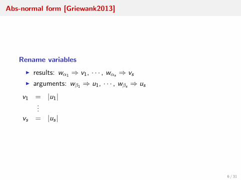
Rename variables

I results: wα1 ⇒ v1, · · · , wαs ⇒ vsI arguments: wβ1 ⇒ u1, · · · , wβs ⇒ us

v1 = |u1|...

vs = |us |

6 / 31

Rewrite the function

Define functions: g : Rn × Rs → Rs , h : Rn × Rs → Rm

u = g(x, v)v = abs(u) componentwise:vk = abs(uk) = |uk |y = h(x, v)

7 / 31

Rewrite function: example

Example1: f (x1, x2) = min(|x1 + x2|, |x1 − x2|), where n = 2,m = 1, min(a, b) = (a + b − |a− b|) ∗ 0.5

Consider the case: x1 = 0.0 and x2 = 0.0 (s = 3)w1 = x1 + x2

w2 = abs(w1)w3 = x1 − x2

w4 = abs(w3)w5 = w2 − w4

w6 = abs(w5)w7 = w2 + w4 − w6

y = w8 = w7 ∗ 0.5

u1 ≡ w1, u2 ≡ w3, u3 ≡ w5,v1 ≡ w2 = |u1|, v2 ≡ w4 = |u2|, v3 ≡ w6 = |u3|.

8 / 31

Rewrite function: example

Example1 (mod): f (x1, x2) = min(|x1 + x2|, |x1 − x2|), wheren = 2, m = 1, min(a, b) = (a + b − |a− b|) ∗ 0.5

Consider the case: x1 = 0.1 and x2 = 0.1 (s = 1)w1 = x1 + x2

w2 = abs(w1)w3 = x1 − x2

w4 = abs(w3)w5 = w2 − w4

w6 = abs(w5)w7 = w2 + w4 − w6

y = w8 = w7 ∗ 0.5

u1 ≡ w3,v1 ≡ w4 = |u1|.

9 / 31

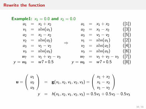
Rewrite the function

Example1: x1 = 0.0 and x2 = 0.0u1 = x1 + x2

v1 = abs(u1)u2 = x1 − x2

v2 = abs(u2)u3 = v1 − v2

v3 = abs(u3)w7 = v1 + v2 − v3

y = w8 = w7 ∗ 0.5

⇒

u1 = x1 + x2 ([1])u2 = x1 − x2 ([3])u3 = v1 − v2 ([5])v1 = abs(u1) ([2])v2 = abs(u2) ([4])v3 = abs(u3) ([6])w7 = v1 + v2 − v3 ([7])

y = w8 = w7 ∗ 0.5 ([8])

u =

u1

u2

u3

= g(x1, x2, v1, v2, v3) =

x1 + x2

x1 − x2

v1 − v2

y = h(x1, x2, v1, v2, v3) = 0.5v1 + 0.5v2 − 0.5v3

10 / 31

Rewrite procedure for linearization

Note that uk = 0.0 for k = 1, 2, 3.

rewrite for linearization∆u1 = ∆x1 + ∆x2

∆v1 = abs(∆u1) = sign(∆u1) ·∆u1 = σ1∆u1

∆u2 = ∆x1 −∆x2

∆v2 = abs(∆u2) = σ2∆u2

∆u3 = ∆v1 −∆v2

∆v3 = abs(∆u3) = σ3∆u3

∆w7 = ∆v1 + ∆v2 −∆v3

∆y = ∆w8 = ∆w7 ∗ 0.5

σk =

{1 if ∆uk > 0−1 if ∆uk < 0

}

11 / 31

Rewrite procedure for linearization

Note that uk = 0.0 for k = 1, 2, 3.

rewrite for linearization∆u1 = ∆x1 + ∆x2

∆u2 = ∆x1 −∆x2

∆u3 = ∆v1 −∆v2

∆v1 = abs(∆u1) = σ1∆u1

∆v2 = abs(∆u2) = σ2∆u2

∆v3 = abs(∆u3) = σ3∆u3

∆w7 = ∆v1 + ∆v2 −∆v3

∆y = ∆w8 = ∆w7 ∗ 0.5

σk =

{1 if ∆uk > 0−1 if ∆uk < 0

}

12 / 31

Differentiation of Absolute function [Griewank2013]

Absolute function

v = |u| = abs(u) = sign(u) · u

v + ∆v = |u + ∆u|= sign(u + ∆u) · (u + ∆u)

= sign(u + ∆u) ·∆u + sign(u + ∆u) · u

∆v = sign(u + ∆u) ·∆u + (sign(u + ∆u)− sign(u)) · u

when u = 0

∆v = sign(∆u) ·∆u = |∆u|

13 / 31

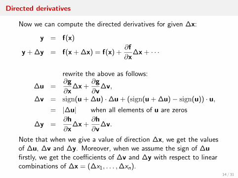
Directed derivatives

Now we can compute the directed derivatives for given ∆x:

y = f(x)

y + ∆y = f(x + ∆x) = f(x) +∂f

∂x∆x + · · ·

rewrite the above as follows:

∆u =∂g

∂x∆x +

∂g

∂v∆v,

∆v = sign(u + ∆u) ·∆u + (sign(u + ∆u)− sign(u)) · u,= |∆u| when all elements of u are zeros

∆y =∂h

∂x∆x +

∂h

∂v∆v.

Note that when we give a value of direction ∆x, we get the valuesof ∆u, ∆v and ∆y. Moreover, when we assume the sign of ∆ufirstly, we get the coefficients of ∆v and ∆y with respect to linearcombinations of ∆x = (∆x1, . . . ,∆xn).

14 / 31

What is my talk

I We check the above concepts with c++ operator overloadprogram for generating computational graph G .

I For a scalar function f (x), we check the first order optimalitycondition (minimization or maximization) by solving LP(Linear Programming) repeatedly.

I The number of solving different LP is O(2s) (naively count)I Reduce the number by branch and bound.

15 / 31

Computation of derivatives

implementation outline

The partial derivatives ∂g/∂x, ∂g/∂v, ∂h/∂x, ∂h/∂v arecomputed as follows.

(i) Make a computational graph G of f as well as the sets ofrenamed nodes, i.e., V = {v1, . . . , vs} and U = {u1, . . . , us}.

(ii) For each node v in V , change the node type of v from thetype that is the result of abs() operation to the type that isthe new independent variable.

(iii) Compute ∂gk/∂xj (j = 1, . . . , n) and ∂gk/∂v` (` = 1, . . . , s)by reverse mode (or forward mode) for all uk ∈ U(k = 1, . . . , s). That is, after the topological sort with thedepth first search from uk , the adjoint values are computedfor all w ≺ uk ∈ G .

(iv) Compute ∂h/∂xj (j = 1, . . . , n) and ∂h/∂v` (` = 1, . . . , s) byreverse mode from the node corresponding to y = f (x).

16 / 31

Representation of ∆v, ∆u, ∆y [Griewank2013]

∆u = (∂g/∂x) ∆x + (∂g/∂v) ∆v∆v = Σ∆u,where Σ ≡ diag(σ1, . . . , σs) is a diagonal matrix.we can eliminate ∆v and get the explicit form ∆u with respect to∆x, that is,∆u = (I − (∂g/∂v) Σ)−1 (∂g/∂x) ∆x.Thus the directed derivative ∆y = (∂f /∂x)∆x is computed by

∆y = (∂h/∂x) ∆x + (∂h/∂v)Σ(I − (∂g/∂v)Σ)−1(∂g/∂x)∆x. (1)

U ≡ (∂g/∂x), L ≡ (∂g/∂v), J ≡ (∂h/∂x) and V ≡ (∂h/∂v).

∆y =(J + VΣ(I − LΣ)−1U

)∆x

17 / 31

Check the local minimum of the linearization

One of key advantages of the abs-normal form is that thecoefficients of a directional derivative ∆y can be computed withthe sign of the ∆u.The sign of the ∆u is computed by the value of the direction ∆x.

Usually

Given ∆x , compute y = f (x)⇒ y + ∆y = f (x + ∆x).

Usually (Abs-normal form)

Given ∆x, compute u = g(x, v), v = |u| ⇒ y = h(x, v)Σ is determined by ∆x∆u = U∆x,∆v = Σ∆u⇒ ∆y = J∆x + V∆v

Fix Σ first(Abs-normal form)

Fix Σ, compute ∆y = J∆x + V∆vCheck the existence of the direction ∆x that realizes the given Σ.

18 / 31

Check the existence of ∆x with respect to Σ

The k-th diagonal element of Σ, σk , indicates the sign of ∆uk .

Check the existence (or finding the subdomain)

I Compute ∆uk as a linear combination of ∆x (k = 1, · · · , s)∆uk > 0 for σk = 1, or, ∆uk < 0 for σk = −1

I Construct an s × n matrix A whose k-th row is ∆uk(ifσk = 1) or −∆uk(if σk = −1)

I Check the feasibility of an LP:min∆x ∆y s.t. A∆x > 0 and − inf < ∆xj < inf

I if it is feasible, there is a direction ∆x that realizes all the signof ∆uk ’s equal to σk ’s.

I if it is not feasible, there is no direction that realizes Σ.

19 / 31

Check the first order condition of locally minimum of the linearization

Check the first order condition of locally minimum of thelinearization

I There are 2s combinations of the values of σk ’s.

I Thus, we can compute a direction that gives ∆y < 0 (or∆y > 0) after solving LP 2s times.

I When we want to know locally minimum (maximum),we check there are no direction that gives ∆y < 0 (∆y > 0).

20 / 31

Algorithm

Algorithm

I (i) Fix a combination of the diagonal values ofΣ = diag(σ1, . . . , σs) = diag(±1, . . . ,±1).

I (ii) Compute ∆u = (I − LΣ)−1U∆x and∆y = (J + VΣ(I − LΣ)−1U)∆x.The coefficients of ∆x1, . . ., ∆xn of the above ∆y may giveone of the generalized gradients.

I (iii) Check the direction ∆x that gives the directed derivative∆y by feasibility of A∆x > 0 with LP

I (iv) Finally, for each matrix A corresponding to all thepossible diagonal matrices Σ, we can check the infeasibility of∆y < 0 and A∆x > 0. When there are no feasible solutionsthe given point x is local minimum or stationary point of thelinearization.

21 / 31

Branch and bound search

I The number of solving LP is at most 2s .I Let a k × n matrix A denote submatrix of A (k ≤ s).

I When A∆x > 0 is feasible, any subsystem of A∆x > 0 shouldbe feasible,

I When A∆x > 0 is infeasible, its extended system A∆x > 0should be infeasible.

I Construct matrix A from the first row to s th row with step bystep (gk indicates the k-th component of g(x, v))

∆u1 =∂g1

∂x∆x

∆u2 =∂g2

∂x∆x +

∂g2

∂v1∆v1 =

∂g2

∂x∆x +

∂g2

∂v1σ1∆u1

· · ·

∆uk =∂gk∂x

∆x +k−1∑j=1

∂gk∂vj

σj∆uj

22 / 31

Branch and bound

Construct sub matrix A(k)

∆uk =∂gk∂x

∆x +k−1∑j=1

∂gk∂vj· σj ·∆uj (k = 1, . . . , s).

After the computation of ∆uk in the explicit form with respect to∆x under the selected sign combination of σ1, . . ., σk , we have∆u1, . . ., ∆uk .Then, we can check the feasibility of A(k)∆x > 0, where the

coefficient matrix is defined by A(k) ≡

σ1∆u1...

σk∆uk

.

I When A(k)∆x > 0 is feasible, we should check A(k+1)∆x > 0is feasible or infeasible for σk+1 = 1 and σk+1 = −1.

I When it is infeasible, there are no feasible solution with thecurrent σ1, . . ., σk . Try the next combination.

23 / 31

Example

Again, f (x1, x2) = min(|x1 + x2|, |x1 − x2|), x1 = 0.0 and x2 = 0.0.

Abs-normal form

∆u =

∆u1

∆u2

∆u3

=

∆x1 + ∆x2

∆x1 −∆x2

∆v1 −∆v2

,

∆v1

∆v2

∆v3

=

σ1∆u1

σ2∆u2

σ3∆u3

,

∆y = 0.5 ∗ (∆v1 + ∆v2 −∆v3)

Partial derivativesWith the forward AD technique, we have

U = (∂g/∂x) =

1 11 −10 0

, L = (∂g/∂v) =

0 0 00 0 01 −1 0

,

J = (∂h/∂x) =(

0 0), V = (∂h/∂v) =

(0.5 0.5 −0.5

).

24 / 31

Explicit ∆y form with respect to ∆x

case: ∆u1 > 0, ∆u2 > 0 and ∆u3 > 0

Σ =

σ1 0 00 σ2 00 0 σ3

=

1 0 00 1 00 0 1

, ∆v1 = ∆u1, ∆v2 = ∆u2,

∆v3 = ∆u3.

The conditions, ∆u1 = ∆x1 + ∆x2 > 0, ∆u2 = ∆x1 −∆x2 > 0and ∆u3 = ∆v1 −∆v2 = ∆u1 −∆u2 = 2∆x2 > 0, hold for∆x1 > ∆x2 > 0.

∆y = (J + VΣ(I − LΣ)−1U)∆x

=

( 0 0)

+(

12

12 − 1

2

) 1 0 00 1 01 −1 1

1 11 −10 0

∆x

=(

1 −1)·∆x = ∆x1 −∆x2.

25 / 31

Figures

-

6

���

@@@

���

@@@

(1)(8)

(4) (5)

(2) (6)

(7) (3)

∆x1

∆x2

26 / 31

Generalized gradient

Table : The generalized gradient ∆y

No. ∆u1 ∆u2 ∆u3 σ1 σ2 σ3 Domain ∆y

(1) > 0 > 0 > 0 1 1 1 ∆x1 > ∆x2 > 0 ∆x1 −∆x2

(2) < 0 > 0 > 0 −1 1 1 0 > ∆x1 > ∆x2 ∆x1 −∆x2

(3) > 0 < 0 > 0 1 −1 1 0 < ∆x1 < ∆x2 −∆x1 + ∆x2

(4) < 0 < 0 > 0 −1 −1 1 ∆x1 < ∆x2 < 0 −∆x1 + ∆x2

(5) > 0 > 0 < 0 1 1 −1 ∆x1 > −∆x2 > 0 ∆x1 + ∆x2

(6) < 0 > 0 < 0 −1 1 −1 0 < ∆x1 < −∆x2 −∆x1 −∆x2

(7) > 0 < 0 < 0 1 −1 −1 0 < −∆x1 < ∆x2 ∆x1 + ∆x2

(8) < 0 < 0 < 0 −1 −1 −1 −∆x1 > ∆x2 > 0 −∆x1 −∆x2

27 / 31

Max-min of planes

Scalar function f (x1, x2) is defined with 2n planes as

f (x1, x2) ≡ max0≤`<n

min(a2`x1 + b2`x2, a2`+1x1 + b2`+1x2).

The k th plane akx1 + bkx2 (k = 0, . . ., 2n− 1) is defined by three points

(pk , qk , rk), (pk+1, qk+1, rk+1) and (0, 0, 0), where

(pk , qk) = (cos(πn k), sin(π

n k)) and arbitrarily given rk((p2n, q2n, r2n) ≡ (p0, q0, r0)).

Figure : Origin is local minimal point28 / 31

Example2-1

n = 32, r2k = 0.3, r2k+1 = 1.0 (k = 0, . . . , 31).Locally minimal point at (0, 0).There are 63 absolute operations whose results are zero, s = 63.The number of solving LP is 2s = 263 ' 1019

the total number of solving LP is only 10340 with the branch andbound search.Computational time is about 7 seconds (Ubuntu14.04LTS, VMware

Fusion 7.1.3, Macbook pro core i7).

Figure : Origin is local minimal point29 / 31

Example2-2

n = 16, r26 = −0.1, r2k = 0.3 (k = 0, . . . , 12, 14, 15), andr2k+1 = 1.0 (k = 0, . . . , 15).The origin (0, 0) is not locally minimal.There are directions along with which the value of f is decreased.There are 31 absolute operations whose results are zero, s = 31.The number of solving LP is 2s = 231 ' 2× 109

the total number of solving LP is only 2222 with the branch andbound search.

Figure : Origin is not local minimal point 30 / 31

Conclusion

Conclusion:

I Simple implementation of piecewise linearization with“abs-normal-form” in C++

I An efficient way to check the local minimal point with branchand bound technique,

I Two dimensional examples that may have 2n planes wereshown, where the number of solving LP is reduced:263 → 10340, 231 → 2222.

Future work:

I More practical experiments and the investigation of theoptimal topological order for the branch and bound are needed

I the investigation of the higher derivatives with absoluteoperations and effects of numerical computational errors.

31 / 31