Simulating and Optimising Design Decisions in Quantitative Goal Models

William Heaven and Emmanuel Letier

Department of Computer Science

University College London {w.heaven, e.letier}@cs.ucl.ac.uk

Abstract—Making decisions among a set of alternative system

designs is an essential activity of requirements engineering. It

involves evaluating how well each alternative satisfies the

stakeholders’ goals and selecting one alternative that achieves

some optimal tradeoffs between possibly conflicting goals.

Quantitative goal models support such activities by describing

how alternative system designs – expressed as alternative goal

refinements and responsibility assignments – impact on the

levels of goal satisfaction specified in terms of measurable

objective functions. Analyzing large numbers of alternative

designs in such models is an expensive activity for which no

dedicated tool support is currently available. This paper takes

a first step towards providing such support by presenting

automated techniques for (i) simulating quantitative goal

models so as to estimate the levels of goal satisfaction

contributed by alternative system designs and (ii) optimising

the system design by applying a multi-objective optimisation

algorithm to search through the design space. These techniques

are presented and validated using a quantitative goal model for

a well-known ambulance service system.

Keywords — requirements simulation and optimisation;

quality requirements; goal-oriented requirements engineering;

quantitative modelling; search-based software engineering

I. INTRODUCTION

Consider a development project to improve the efficiency of an existing system. Stakeholders and designers have identified several alternative ways that improvements might be achieved and you have to guide them in making the best decisions about which of these alternatives ought to be selected for implementation. Imagine, for example, an ambulance dispatching system for the London Ambulance Service (LAS) [1][2]. This system must ensure that ambulances respond to reported incidents across the city as swiftly as possible. Alternative options for improving the system include improving some of the call-taking features of the software so that details about reported incidents can be encoded faster and more accurately; replacing ambulance radios with mobile data terminals so that more information can be communicated directly to the ambulance crews; and improving the speed and accuracy of ambulance-allocation decisions by automating all or part of the allocation process. These alternatives have different costs and different impacts on the system goals. A key goal in this example is to maximize the 14 minute response rate, that is, the percentage of incidents for which the first ambulance arrives at the incident scene within 14 minutes of the first call. This goal

comes from a 1992 UK Government standard requiring the 14 minute response rate to be above or equal to 95 %. Being able to estimate how much each alternative option would contribute to improving the 14 minute response rate would help decision makers make informed decisions between the alternative options.

In previous work, we have presented a quantitative goal modeling framework for specifying goals with measurable objective functions and modeling the impact that alternative system designs have on these goals [3]. This framework extends the KAOS goal modeling language [4] with a probabilistic layer allowing one to specify and reason about measurable quantitative requirements in the spirit of the VOLERE [5] and Planguage methods [6]. The work presented there motivates the need for quantitative goal models based on measurable goal definitions, defines the language‟s formal semantics, and presents a set of heuristics for the systematic elaboration of such models. It does not consider how to automate the model analysis. It gives an illustration of how quantitative goal models can be used to compare three alternative system designs for an ambulance despatching system. This analysis was done following an ad-hoc process using a mix of analytical and numerical methods. The process used there is error-prone, labour intensive, and does not scale to very large numbers of design alternatives. Our objective in this paper is to address these limitations by presenting automated techniques for evaluating large numbers of design alternatives and identifying the optimal ones among them.

The paper presents a simulation and optimisation framework for evaluating the impact of alternative system designs on high level goals and for finding optimal design options among the alternatives. Given a quantitative goal model, our technique generates a stochastic simulation model able to simulate the whole range of alternative designs in the goal model. The simulation takes as input a particular set of design choices and a sample size to be simulated (for example the number of incidents to be simulated), it then uses the probability distributions and equations of the quantitative goal model to simulate the behaviour of that particular design and compute the levels of goal satisfaction obtained for that simulation. This simulation model is then used by a multi-objective optimization component that searches through the design space in order to identify the optimal design choices.

The techniques are illustrated on the London Ambulance Service goal model for which a prototype simulation model – implemented in Matlab – is generated manually (but

systematically) from the goal model and the NSGAII genetic algorithm is used to search through the design space. The case study shows the potential of simulation and optimisation techniques in providing sound decision making tools for requirements engineering and highlights the need for improved optimization algorithms for exploring alternative design options in such goal models.

II. BACKGROUND

A. Goal-Oriented RE with KAOS

Goal-oriented requirements engineering is a popular paradigm for eliciting, modelling, and reasoning about system requirements [4]. Goals are prescriptive statements of intent that the system should satisfy through the cooperation of its agents. Agents are active system components playing specific roles in the goals satisfaction. Agents include human agents, software components, and hardware devices such as sensors and actuators. Goals can be AND/OR refined into subgoals. An AND-refinement relates a parent goal to a set of subgoals; it means that the satisfaction of all subgoals ensures the satisfaction of the parent goal in the application domain. An OR-refinement relates a parent goal to a set of alternative AND-refinements; it means that any one of the alternative AND-refinements is sufficient for satisfying the parent goal. OR-refinements are used to model alternative design choices for satisfying the parent goal. Goals are AND-refined into subgoals until the resulting subgoals can be assigned as the responsibility of single agents. Assigning a goal to an agent means that the agent is the only one required to restrict its behaviour to ensure the goal‟s satisfaction. OR-responsibility assignments are used to model alternative assignment of goals to agents. These correspond to alternative design choices, for example of assigning a goal to a human or automated agent.

Figure 1 shows portion of a goal model built for the London Ambulance Service (LAS) case study [3], which was based on the report from the inquiry following a major system failure [1]. The top-level goal in this figure, Achieve

[Ambulance Intervention], requires that a first ambulance arrives at the incident scene within 14 minutes after the first call.

Goal specifications include a natural language definition and an optional formal specification in Linear Temporal Logic. The goal Achieve [Ambulance Intervention] is AND-refined into the subgoals Achieve [Ambulance Mobilisation] and Achieve

[Mobilised Ambulance Intervention]. The goal Achieve [Ambulance

Mobilised] requires that an ambulance be mobilised to an incident within 3 minutes after the first call and that the mobilised ambulance is less than 11 minutes away from the incident. The goal Achieve [Mobilised Ambulance Intervention] requires that once an ambulance is mobilised for an incident location it will reach that location without delay.

Options correspond to alternative choices at decision points in the goal model, where a decision point is either an OR refinement or an OR responsibility assignment (other decision points related to conflict and obstacle resolutions [2][7] are not considered in this paper). Options correspond to the system reference attribute attached to goal refinements, responsibility assignments, and obstacle resolutions in the KAOS meta-model [4]. To save space, in Figure 1 we show the options without showing the alternative goal refinements or responsibility assignments that define them. In this model, the goal Achieve [Incident Form Encoded] has four alternative options for its satisfaction. The first corresponds to the current paper based-system (in 1992), the second corresponds to using an computer-based call tacking system, the third consists in using an automated system for locating calls, and the fourth consists in using a computer-based call taking system with automated call location. Options for satisfying the goal Achieve [Ambulance Allocated] are to use the current radio-based system, or to use mobile data terminals on board of ambulances of which two different systems could be chosen, system A or B.

B. Quantitative Goal Models

We have previously developed an extension of the KAOS framework for reasoning about alternative design choices based on measurable, domain-specific criteria [3]. In this framework, the degrees of satisfaction for a goal are specified using objective functions defined in terms of quality variables, which are random variables (i.e. functions over probability spaces). For example, we can specify the

Ambulance Intervention

Ambulance Mobilized Mobilized Ambulance Intervention

Incident Form Encoded Ambulance Mobilized Based on Incident Form

Option 1.1.Curent paper-based

Option 1.2. Computer-based call taking

Option 1.3. Automated Call Location

Option 1.4. Computer-based + automated location

Ambulance Allocated Based on Incident Form

Allocated Ambulance Mobilised

Ambulance Allocated Based on Incident Form and Ambulance Info

Option 2.1. Current Radio-based

Option 2.2. MDT- System A

Option 2.3. MDT- System B

Accurate Ambulance Info

Option 3.1. Current radio and paper-based

Option 3.2. Automated Vehicle Location (A)

Option 3.3. Automated Vehicle Location (B)

Option 4.1. Current paper-based

Option 4.2.Interactive Allocation

Option 4.3.Fully Automated Allocation

Figure 1. Partial goal model for the LAS system showing decision points for alternative system designs

goal Achieve [Ambulance Intervention] as follows:

Goal Achieve [Ambulance Intervention]

Definition

For every urgent call reporting an incident, there should be an ambulance at the incident scene within 14 minutes after receiving the first call.

Formal Definition ( i:Incident, c: UrgentCall)

Reporting(c, i) ײ14mins ( a:Ambulance) Intervention(a,i)

Objective Functions

14MinResponseRate = MAX [ P(ResponseTime 14 mins) ] 8MinResponseRate = MAX [ P(ResponseTime 8 mins) ]

Quality Variable

ResponseTime: Incident -> Time {def: the duration in seconds between the start of the first call reporting the incident and the arrival of the first ambulance at the incident scene.}

The goal‟s definition and formal definition define what it means for the goal to be satisfied in an absolute sense; the goal semantic is the set of system behaviours – i.e. sequences of system states – that satisfy the goal‟s formal definition. The goal objective functions define the measures to be used for assessing partial levels of goal satisfaction. Objective functions are defined in terms of quality variables that correspond to domain phenomena related to the goal‟s definition. In this example, the quality variable is the incident response time, and the objective functions are the probability that the response time is less than 14 minutes and 8 minutes, respectively. In this example, both objective functions have to be maximized. For the actual LAS system, the target values for these objective functions are Government standards that in 1992 were set at 95% and 50%, respectively. The specification of adequate objective functions is one of the most critical steps of a system design. Designing an ambulance system to optimize these objective functions is likely to yield a very different system than one whose only objective function would be to minimize the mean response time for example.

The quality variables associated with a goal can be related to quality variables associated with its subgoals through domain-specific refinement equations. For example, the quality variable response time is related to the quality variables MobilisationTime, MobilisationDistance, and

AmbulanceDelay of the goals Achieve [Ambulance Mobilisation]

and Achieve [Mobilised Ambulance Intervention] through the following refinement equations:

ResponseTime =

MobilisationTime + MobilisationDistance + AmbulanceDelay.

The variable MobilisationTime denotes the time it takes to mobilize the first ambulance, MobilisationDistance denotes the time-distance between the mobilised ambulance and the incident location (e.g. the ambulance is 11 minutes away from the incident), and AmbulanceDelay denotes the difference between the mobilisation distance and the actual time taken by the ambulance to reach the incident location. Figure 2 shows the goals‟ quality variables for the portion of the goal model in Figure 1.

Quality variables can be of any type, they are not restricted to a time domain. For example, in the LAS model the goal Achieve [Ambulance Intervention] has an additional Boolean quality variable

IncidentDropped: Incident -> Boolean

that is true of reported incidents for which no ambulance ever arrives at the incident scene [3]. The associated objective (not shown in the example above) is to minimize the probability that an incident is dropped. This quality variable can be related to quality variables of subgoals through the following equation involving other Boolean quality variables:

IncidentDropped = NoAmbulanceMobilisedWrongMobilisationDestination AmbulanceInterventionFailure.

Goals quality variables are thereby recursively related to other quality variables along the goal refinement links until reaching goals assigned to the responsibility of single agents. Quality variables attached to a goal assigned to a single agent can be further related to quality variables attached to obstacles to that goal. An obstacle to a goal is a condition that violates the goal [2]. For example, AmbulanceDelay could be a function of the quality variables AmbulanceBreakdown, TrafficLevel, and AmbluanceLost attached to obstacles to the

Ambulance Intervention

Ambulance Mobilised Mobilised Ambulance Intervention

Incident Form Encoded Ambulance Mobilised Based on Incident Form

Ambulance Allocated Based on Incident Form Allocated Ambulance Mobilised

ResponseTime

AmbulanceDelay MobilisationTime MobilisationDistance

MobilisationCommunicationTime

CallTakingTime DistanceMobilised Ambulance

MobilisationTime AfterFormEncoding

AllocationTime DistanceAllocatedAmbulance

Figure 2. Quality variables for the LAS goal model

goal Achieve [Mobilized Ambulance Intervention] [3]. The handling of quality variables and refinement equations on obstacles is the same as for quality variables attached to goals and therefore does not require a special treatment when simulating the model.

Quantitative goal models can be used to evaluate the expected value for the goals‟ objective functions in alternative system designs. This evaluation requires an estimation of the probability distribution function for each leaf quality variable in the model. For example, the variable CallTakingTime – denoting the time it takes to fill in the incident form after the start of the first call– could be characterized as having an exponential distribution whose mean varies from 60 seconds to 30 seconds depending on which option is selected for satisfying the goal:

CallTakingTime = Exp(60) if Option 1.1 is selected Exp(40) if Option 1.2 is selected Exp(45) if Option 1.3 is selected Exp(30) if Option 1.4 is selected

Estimating the probability distributions of leaf quality variables can be done in various ways; it can for example be inferred from statistical data about the existing system or be constructed from expert judgement about the future system. An important distinction is to be made between descriptive, predictive, and prescriptive probability distributions. A descriptive distribution is one that describes characteristics of the existing system, a predictive distribution is one that predicts some characteristics for the future system, and a prescriptive distribution is one that prescribes some characteristics for the future system. For example, the probability distribution for CallTakingTime is descriptive for Option 1.1 because it describes how long it takes to write down call details on incident form in the existing paper-based system. It is predictive for Option 1.2 because it predicts how long it will take to call takers to encode incident details using an existing computer-based call tacking system. It is prescriptive for Option 1.3 because it prescribes how the automated call location feature should contribute to reducing the call taking time. The probability distribution for Option 1.2 could also be seen as prescriptive if it is meant to impose a requirement to be met by the designers of the computer-based call taking system.

Unlike probabilistic transition systems and model checkers [8], the model is not restricted to random variables with exponential distributions. Any distribution function can be used. For example, the quality variable AmbulanceDelay could be characterized as having a normal distribution with a mean of 0 and standard deviation of 120 seconds: AmbulanceDelay = Normal(0, 120).

Computing objective functions from leaf quality variables and refinement equations rely on the assumption that the leaf quality variables are statistically independent. This assumption –also used in quantitative fault trees and Bayesian networks– is required to ensure correctness of the computations (it allows the probability of two events – e.g. that the call taking time for an incident is less than 1 minute and its ambulance allocation time less than 2 minutes – to be computed as the product of the probability of each event).

The stochastic simulation process we present in the following section relies on this assumption because it generates simulated values for each quality variable according to its probability distribution function independently from other variables simulations. If the system analysts suspect that the independence assumption between leaf quality variables does not hold, they have to elaborate the model by refining the quality variables further until reaching leaf quality variables that can be considered to be independent.

Systematic techniques for elaborating quantitative goal models have been proposed [3]. These include heuristics for deriving a goal's quality variables and objective functions from the goal's definition, patterns of refinement equations, and guidance on how to reach a set of independent leaf quality variables.

III. EVALUATING ALTERNATIVES WITH STOCHASTIC

SIMULATION

The problem we address is how to evaluate and compare degrees of goal satisfaction contributed by alternative system designs. In the context of our quantitative goal model, the problem is thus how to compute the objective functions for the higher-level goals given the refinement equations and estimates of the probability distributions for all leaf quality variables. The problem is particularly complex because our models allows any refinement equations (they are not restricted to linear functions such as weighted sums) and leaf quality variables can have any distributions (they are not restricted to a single distribution type).

Our previous approach for computing objective functions involved transforming the quality variable refinement equations into equations relating the quality variables probability density functions, which are integral equations that we resolved using numerical techniques [3]. This process is labour-intensive, error-prone, and does not scale to the evaluation of large number of alternatives.

The approach described in this paper overcomes these limitations by generating a stochastic simulation model from the quantitative goal model. The stochastic simulation model simulates each alternative system design by generating sample values for each leaf quality variables according to its probability distribution in a chosen design option and computes the objective functions values obtained in that simulation. An additional benefit of this approach is that it generates simulated values for all quality variables that could then be analysed to gain further insights in the system behaviour than just computing its objective functions.

A. Simulating Goal Models

Our simulation process can be described as the function

SimulateGoal :G × N→ Gsim

that takes as input a goal G for which an objective function is defined and a parameter N specifying a sample size for the quality variables in the model, and generates a structure Gsim consisting of a goal graph rooted at G (i.e. G and all transitively related sub-goals) in which approximate values have been computed for all objective functions and

simulated values generated for all quality variables. If the model contains quality variables with different domains, separate sample sizes can be specified for each.

For example, we might simulate our top-level goal Achieve [Ambulance Intervention] with a sample size of 1000, i.e. we would simulate the goal for 1000 incidents since this is the domain for the quality variables of the model (e.g. ResponseTime: Incident → Time). The procedure call

SimulateGoal(Ambulance Intervention, 1000)

then generates a goal graph rooted at this top-level goal for which we have computed

a vector of 1000 simulated values for each quality variable in this goal graph, e.g. ResponseTime = [v1, v2, ..., v1000]

simulated values for the goal's two objective functions computed using the 1000 simulated values for ResponseTime.

Our simulation algorithm computes the quality variables and objective functions simulated values by traversing the goal graph recursively from the top-level goals. Since a goal model is a directed acyclic graph, we must ensure that a goal is not simulated twice for the same instances in the quality variable sample space (e.g. we must avoid generating two different vectors of simulated values of CallTakingTime for the same incidents). To achieve this, the algorithm stores the results of goals that have already been simulated in a data structure Gsim. The procedure for simulating a goal G is composed of the following steps:

1. If G has subgoals (or obstacles), simulate each subgoal (or obstacle) that has not already been simulated, i.e. that is not already in Gsim.

2. For each leaf quality variable in G (if any), generate its vector of N simulated values using its probability distribution in the simulated design option.

3. For each non-leaf quality variable in G (if any), compute its vector of sample values using its refinement equation and the simulated values for the quality variables involved in that equation.

4. If the goal has objective functions, compute the objective functions simulated values from the quality variables simulated values.

5. Add the goal and its simulated quality variables and objective functions to Gsim.

Our simulation model for the LAS quantitative goal model is implemented in Matlab. We use Matlab built-in functions to generate sample values for all leaf quality variables. For example, the Matlab command

CallTakingTime = exprnd(meanCallTakingTime, 1, N)

generates a vector CallTakingTime of N random numbers from an exponential distribution with mean of meanCallTakingTime. Each value in this vector represents the call taking time for one particular incident. The quality variables refinement equations are then applied to the vectors of sample quality variable values using the usual element-wise vector operations. For example, the equation

ResponseTime = MobilisationTime + MobilisationDistance + AmbulanceDelay

generates an N-dimension vector obtained from the element-wise addition of the three vectors in the right hand side of the equation. Simulated values for the goals‟ objective functions are computed from the simulated vectors for the goal‟s quality variables using the frequentist interpretation of probabilities. For example, the 8 minutes and 14 minutes response rate defined in Section II are computed as the percentage of simulated response time that is below 8 and 14 minutes, respectively:

8MinResponseRate = sum(ResponseTime<= 8 min)/N 14MinResponseRate = sum(ResponseTime<=14 min)/N

where N is the number of simulated incidents. In addition to the LAS simulation, we have also

developed a simulation model for a financial fraud detection system based on a quantitative goal model for that system [9][10]. This simulation is implemented in R, a mathematical programming environment that provides the same high-level mechanisms for random variable generation and vector manipulation as Matlab.

Using these high-level mathematical environments allowed us to build quick prototypes for the simulation models and to easily connect these models to existing optimization algorithms as will be described in Section IV. The goal-based, recursive structure of our simulation technique could equally be implemented in faster, procedural programming languages. Ideally, future work should automate the generation of the simulation models from quantitative goal models.

B. An Example Simulation

As an example let us compute approximate values for the objective functions 8MinResponseRate and 14MinResponseRate for the current system in Figure 1, i.e. the system defined by selecting options 1.1., 2.1, 3.1, and 4.1. In addition to providing a benchmark against which to judge potential improvement, simulating the existing system design can be a useful exercise in practice since it may be possible to compare the approximate values computed for the objective functions with actual values measured for the real system, thereby validating the quantitative goal model. We can also assume that good estimates of the expected values and probability distributions for the quality variables in question are known for the current system. Let us assume the estimated distribution functions for the leaf quality variables in Figure 1 are defined as follows (time is measured in seconds):

CallTakingTime = Exp(60) AmbulanceDelay = Normal(0, 120) AllocationTime = Exp(60) MobilisationCommunicationTime = Exp(60)

The quality variable DistanceAllocatedAmbulance, denoting the time-distance between the incident location and the ambulance allocated to the incident, depends on the quality variables denoting the number of ambulances, the frequency of incidents, the city size, the error in ambulance location and availability information, and error in the allocation decision process attached to lower-level goals and domain properties not shown in Figure 1.

For this example, a simulation run with 1000 incidents computes the expected values for the 8 and 14 minutes response rate to be 61% and 97%, respectively. These rates are both above the government standard. However, we may still be interested in finding improvements. Running the simulation again but this time selecting the second option for Achieve [Ambulance Allocated Based On Incident Form], which allocates responsibility for the goal to a software agent instead of a human operator, giving an estimated mean Allocation Decision Time of only 5 seconds, we see an improved approximate value for 8MinReponseRateof 73%. This simulation returns a result in about a second on an average desktop machine.

C. Setting the simulation size to a confidence interval

Because our model involves probabilistic variables, the simulation of a particular system design is non-deterministic and the simulated value for its goals‟ objective functions may not correspond to their exact values for the model. The deviation between an objective function simulated value and its exact value will decrease as the size of the sample space used during the simulation increases. This deviation can be assessed using the common statistical measures of standard error and confidence interval. We have used such measures to allow goal simulation to incrementally increase the sample size to be simulated until reaching a confidence interval of 95% (or some other desired target) on all top-level objective functions.

IV. SEARCHING FOR OPTIMAL TRADEOFFS IN MULTI-

OBJECTIVE DESIGNS

We have seen how stochastic simulation can be used to evaluate alternative system designs. However, by itself, the simulation-based approach we have described still requires comparisons between distinct design choices to be assessed manually. For example, simulations could be run individually for two separate designs and the results compared by hand, with the engineer opting for the design that gives the better degrees of satisfaction across the important goals of interest. But teasing out the subtleties of different tradeoffs between multiple competing goals is not straightforward. More importantly the design space of distinct alternative system designs grows exponentially with the number of individual design choices. For example, if we have 2 goals each with 3 possible OR-refinements we have 9 potential system designs to evaluate, and if we add just 2 more goals, each with 4 alternative refinements, we have 144 designs (assuming these alternatives are neither mutually inconsistent nor mutually dependent, which would constrain the design space somewhat). Techniques are therefore needed to guide the evaluation and comparison of large numbers of alternative system designs in goal models.

A. Multi-Objective Optimisation Problems

The problem to be solved is a multi-objective optimization problem because design choices must take into account multiple stakeholders‟ goals that are not directly comparable one to another. For example, for the LAS, the objectives of maximizing the 14 minutes and 8 minutes

response rates must be balanced against an objective of minimising costs. For a plastic card fraud detection system, the objective of minimizing undetected frauds must be balanced against the objective of minimizing false alerts that result in cards being blocked unnecessarily. These two objectives are themselves related to conflicting goals at a higher-level in the goal model such as minimizing financial loss due to fraud, minimizing card holders‟ inconvenience, and minimizing fraud investigation costs. In general, there is not a single design that is better than all others for all objectives simultaneously.

Formally, the problem consists in selecting options for all decision points in the goal model, i.e. for all alternative goal refinements and responsibility assignments, so as to optimize the set of objective functions {OF1, ..., OFn} attached to the models‟ top-level goals. If there are M decision points, a particular system design can be represented as a vector d =

[d1, ..., dM] where di represents the choice made for decision point i. The objective function OFi for a particular system design d = [d1, ..., dm], noted OFi(d), is computed by simulating the goal model for this set of design options. A system design d is said to dominate a system design d’ if and only if it performs better than d’ for at least one objective function and performs as least as well as d’ for all other objective functions:

OFi(d) >OFi(d') for some i in 1..n

OFi(d) ≥OFi(d') for all i in 1..n.

(This formulation assumes that all objective functions have to be maximized. An objective function that has to be minimized can always be transformed into one that has to be maximised by reversing its sign.) A system design is said to be Pareto-optimal if it is not dominated by any other system design. The set of Pareto-optimal solutions is therefore composed of all “best” designs from the goal model. Allowing decision makers to explore this set helps them to identify what can be achieved and to select one design in that

G

G1 G2

G1.2 G1.1 G1.2 G1.1

refinement A refinement B OR

Ag1 Ag2 Ag3

Responsibility

(XOR)

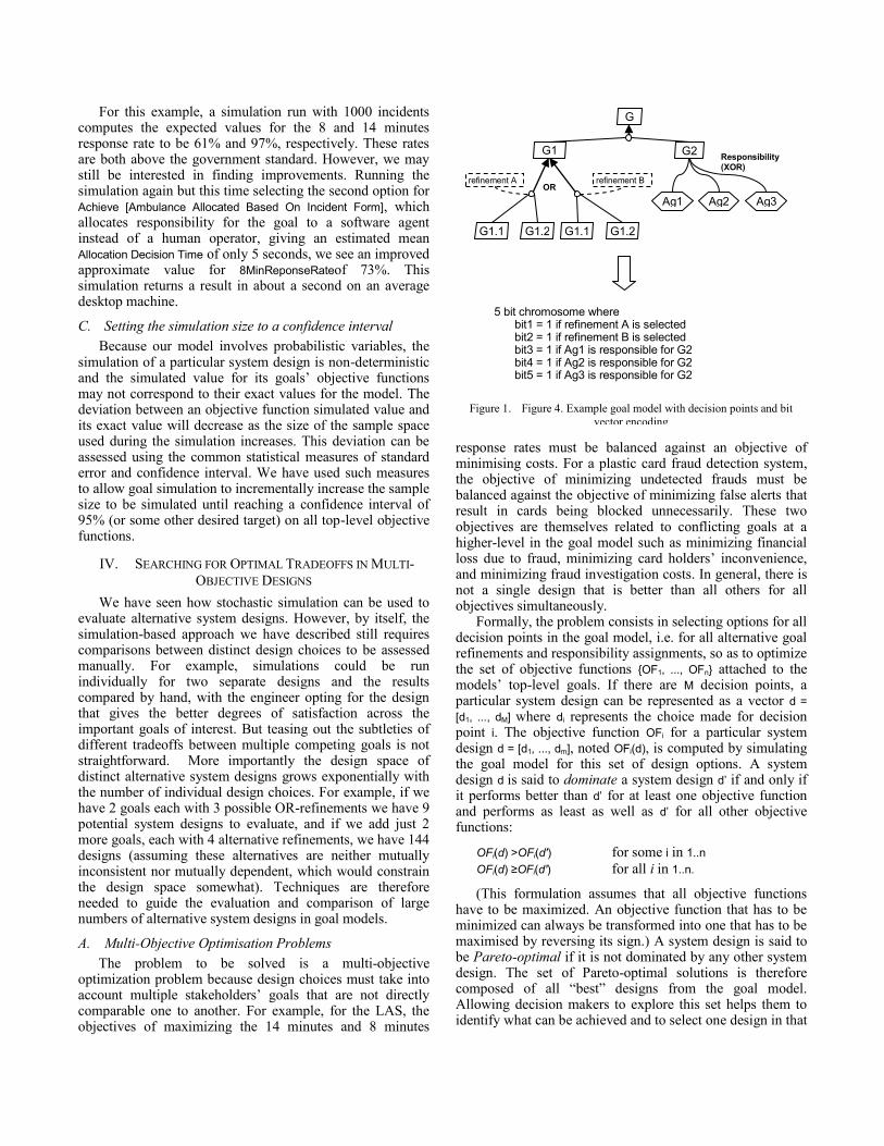
5 bit chromosome where bit1 = 1 if refinement A is selected bit2 = 1 if refinement B is selected bit3 = 1 if Ag1 is responsible for G2 bit4 = 1 if Ag2 is responsible for G2 bit5 = 1 if Ag3 is responsible for G2

Figure 1. Figure 4. Example goal model with decision points and bit

vector encoding

set that corresponds to an appropriate trade-off between the multiple objectives.

One approach to solving a multi-objective optimization problem is to transform it into a single objective problem by aggregating all objectives into a single one defined as the weighted sum of the individual objectives. This approach, however, requires the a priori elicitation of the objective functions weights –which are subjective and without physical interpretation in the application domain– and produces as output a single element in the set of Pareto-optimal solutions instead of allowing decision makers to explore the full set of such solutions [11].

B. Multi-Objective Optimization Algorithms

Our aim in this section is to explore the use of out-of-the-box multi-objective optimization techniques for exploring alternative system designs in goal models. Standard techniques such as Integer Linear Programming will in general not be applicable because objective functions and quality variable refinement equations are not restricted to linear functions. A suitable approach in our context is to use meta-heuristic search algorithms to let the objective functions guide the search through the design space. Such algorithms are used increasingly to solve optimization problems in different areas of software engineering [11]. For the LAS case study, we have used NSGA-II [12] which is a state-of-the-art genetic algorithm that has an implementation in Matlab‟s Global Optimization Toolbox. We here briefly sketch the basic mechanisms of such an algorithm necessary to understand how to map the search for optimal design decisions in goal models to an adequate representation allowing such algorithm to be used.

Genetic search-based algorithms converge on a solution over the course of a number of iterations, known as generations. In our case, a solution would be a set of Pareto optimal designs. Each generation a candidate approximation of the real solution – known as that generation‟s population – is selected and each member of the population – known as a chromosome – is evaluated via a fitness function, which ranks the chromosomes according to given criteria. For multi-objective optimisation we would rank highly those chromosomes that represent a value that is dominated by no (or relatively few) others in the population. We evaluate alternative chromosomes (design choices) based on the approximate values they contribute to objective functions. The next generation‟s population is then selected from the highest ranking chromosomes of the current population by a customisable process known as crossover, which splices parts of two parent chromosomes together to create a new one that inherits characteristics of both parents. Typically, a certain number of the highest ranking chromosomes will also survive through to the next generation. The key feature of this algorithm is that exploration of the search space is guided by the fitness function since it determines the direction in which the search proceeds by selecting the best candidates for crossover.

C. Encoding the Optimisation Problem for Design Choices

Genetic algorithms like NSGAII represent chromosomes using a binary representation, i.e. each chromosome is represented as a vector of bits. In order to use such algorithm to explore alternative design choices in goal models, we therefore need to define a mapping from alternative system designs in the goal model to a binary representation. Figure 4 illustrates this mapping for a small general example. Here the goal model has five decision points which we encode with a five-bit vector in which 1 (resp. 0) indicates that the design option represented by that bit is selected (resp. not selected). Further constraints on the selection of design choices, such as exclusive alternatives or mutual dependencies between design options are captured by logical constraints over these bit vectors. For example, in each system design a goal can be assigned as the responsibility of at most one agent. In our example, this means that bits 3 to 5 in a chromosome are mutually exclusive.

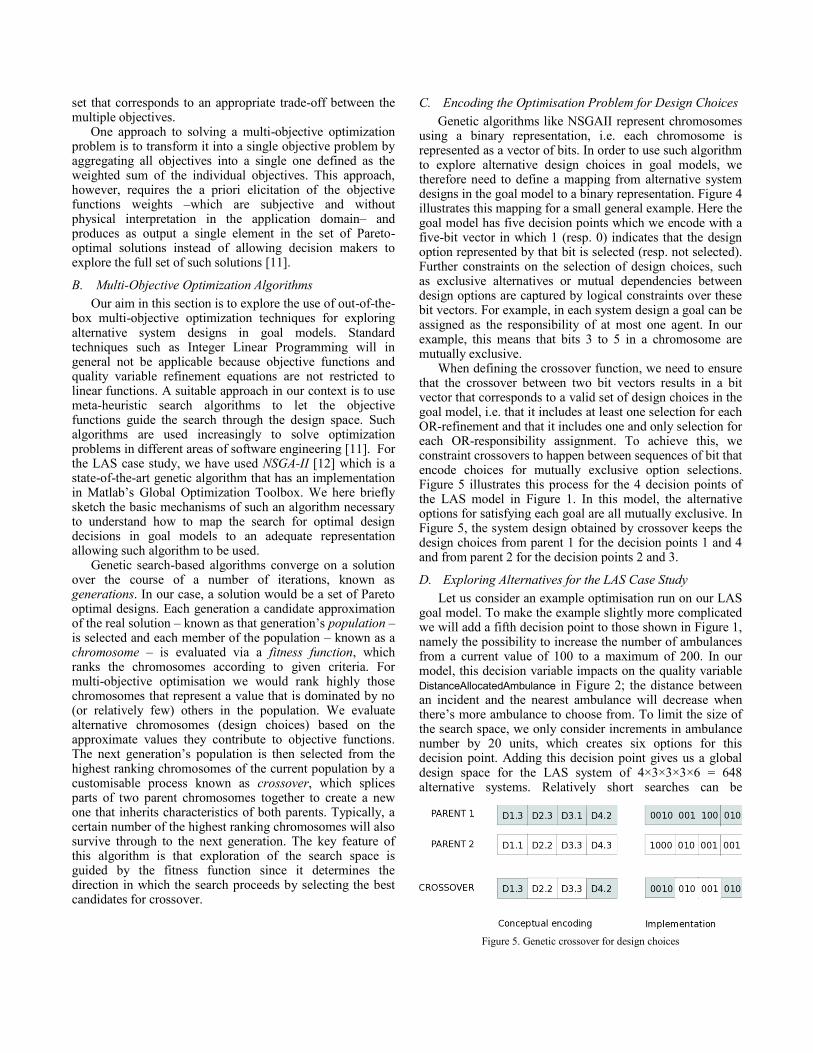
When defining the crossover function, we need to ensure that the crossover between two bit vectors results in a bit vector that corresponds to a valid set of design choices in the goal model, i.e. that it includes at least one selection for each OR-refinement and that it includes one and only selection for each OR-responsibility assignment. To achieve this, we constraint crossovers to happen between sequences of bit that encode choices for mutually exclusive option selections. Figure 5 illustrates this process for the 4 decision points of the LAS model in Figure 1. In this model, the alternative options for satisfying each goal are all mutually exclusive. In Figure 5, the system design obtained by crossover keeps the design choices from parent 1 for the decision points 1 and 4 and from parent 2 for the decision points 2 and 3.

D. Exploring Alternatives for the LAS Case Study

Let us consider an example optimisation run on our LAS goal model. To make the example slightly more complicated we will add a fifth decision point to those shown in Figure 1, namely the possibility to increase the number of ambulances from a current value of 100 to a maximum of 200. In our model, this decision variable impacts on the quality variable DistanceAllocatedAmbulance in Figure 2; the distance between an incident and the nearest ambulance will decrease when there‟s more ambulance to choose from. To limit the size of the search space, we only consider increments in ambulance number by 20 units, which creates six options for this decision point. Adding this decision point gives us a global design space for the LAS system of 4×3×3×3×6 = 648 alternative systems. Relatively short searches can be

Figure 5. Genetic crossover for design choices

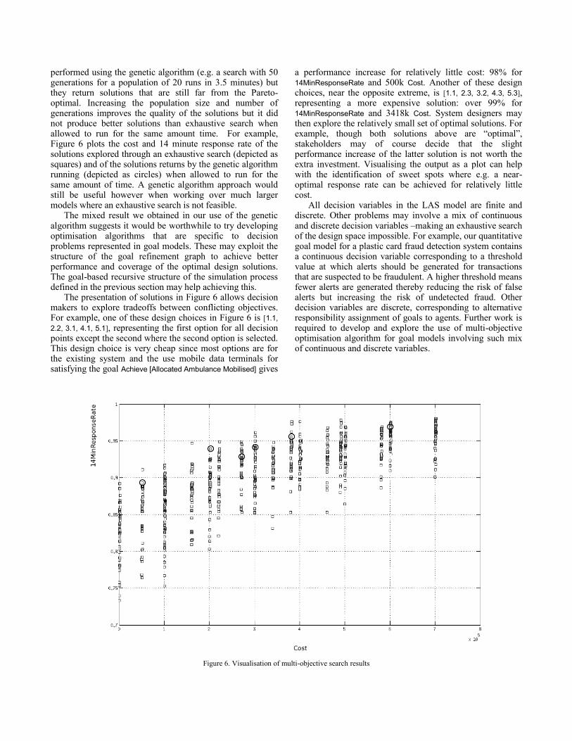
performed using the genetic algorithm (e.g. a search with 50 generations for a population of 20 runs in 3.5 minutes) but they return solutions that are still far from the Pareto-optimal. Increasing the population size and number of generations improves the quality of the solutions but it did not produce better solutions than exhaustive search when allowed to run for the same amount time. For example, Figure 6 plots the cost and 14 minute response rate of the solutions explored through an exhaustive search (depicted as squares) and of the solutions returns by the genetic algorithm running (depicted as circles) when allowed to run for the same amount of time. A genetic algorithm approach would still be useful however when working over much larger models where an exhaustive search is not feasible.

The mixed result we obtained in our use of the genetic algorithm suggests it would be worthwhile to try developing optimisation algorithms that are specific to decision problems represented in goal models. These may exploit the structure of the goal refinement graph to achieve better performance and coverage of the optimal design solutions. The goal-based recursive structure of the simulation process defined in the previous section may help achieving this.

The presentation of solutions in Figure 6 allows decision makers to explore tradeoffs between conflicting objectives. For example, one of these design choices in Figure 6 is [1.1,

2.2, 3.1, 4.1, 5.1], representing the first option for all decision points except the second where the second option is selected. This design choice is very cheap since most options are for the existing system and the use mobile data terminals for satisfying the goal Achieve [Allocated Ambulance Mobilised] gives

a performance increase for relatively little cost: 98% for 14MinResponseRate and 500k Cost. Another of these design choices, near the opposite extreme, is [1.1, 2.3, 3.2, 4.3, 5.3], representing a more expensive solution: over 99% for 14MinResponseRate and 3418k Cost. System designers may then explore the relatively small set of optimal solutions. For example, though both solutions above are “optimal”, stakeholders may of course decide that the slight performance increase of the latter solution is not worth the extra investment. Visualising the output as a plot can help with the identification of sweet spots where e.g. a near-optimal response rate can be achieved for relatively little cost.

All decision variables in the LAS model are finite and discrete. Other problems may involve a mix of continuous and discrete decision variables –making an exhaustive search of the design space impossible. For example, our quantitative goal model for a plastic card fraud detection system contains a continuous decision variable corresponding to a threshold value at which alerts should be generated for transactions that are suspected to be fraudulent. A higher threshold means fewer alerts are generated thereby reducing the risk of false alerts but increasing the risk of undetected fraud. Other decision variables are discrete, corresponding to alternative responsibility assignment of goals to agents. Further work is required to develop and explore the use of multi-objective optimisation algorithm for goal models involving such mix of continuous and discrete variables.

Figure 6. Visualisation of multi-objective search results

V. RELATED WORK

There exist many requirements engineering techniques to guide the selection among alternative system designs. Qualitative techniques such as the NFR framework [13] and Win-Win model [14] allow one to reason about the positive or negative influences of alternative design options on goals, but the qualitative information contained in these models is generally insufficient to make informed decisions. Numerous quantitative techniques have been proposed with the aim of providing more detailed information on which to base requirements decisions. These include NASA‟s DDP framework [15], the house of quality matrix in the QFD method [16], and quantitative extensions to goal models in the NFR, KAOS, and GRL frameworks [17][18][19]. However, more detailed does not necessarily mean more accurate. A major problem with the above techniques is that there is no way to check the accuracy of the quantitative models against the real-world system they represent because the quantities they manipulate have no physical interpretation in the application domain [3]. For example, specifying that the impact of a computer-based call taking system on the LAS performance goal is 7 whereas the impact of an automated call location system is 5 tells us that stakeholders believe the first option is slightly better than the second but, because these numbers have no meaning in the application domain, there is no way of checking the validity of that belief. This contrasts with the quantitative approaches where level of goals satisfaction have a concrete physical interpretation such as VOLERE fit criteria [5], Planguage quantified requirements [6] and performance indicators used in organization management and recently introduced in the User Requirements Notation [20][21]. Our quantitative goal modelling framework provides formal foundation for reasoning about measurable levels of goal [3]. This paper extends this framework with automated techniques for simulating and optimizing the design decisions in such models. These techniques allow one to simulate large numbers of alternative systems designs more efficiently and systematically than the initial ad-hoc process of [3] that relied on transforming refinement equations into integrals on quality variables probability density functions.

The multi-objective search-based optimization technique proposed in this paper can be seen as an alternative and extension to the backward propagation algorithms on qualitative and quantitative goal models [22][19]. These algorithms allow one to explore whether there exist sets of design alternatives in a goal model that satisfy top-level goals to acceptable levels but not to search for optimal design alternatives among them.

Probabilistic models such as queuing models, Markov models, reliability block diagrams, fault trees, and event trees provide standard techniques to evaluate performance, reliability, and availability goals [23]. Our quantitative goal modelling framework [3] differs from probabilistic transition systems in several ways: it is goal-based and declarative instead of being operational, it allows for compositional reasoning with respect to the goal structure, and it allows for a variety of probability distribution function to be used

whereas exponential distributions only are used in probabilistic transition systems. These differences imply entirely different simulation techniques than the ones used for probabilistic transition systems [8].

Bayesian Belief Networks (BBNs) provide alternative models for evaluating and making decisions among alternative system designs [24]. They are however limited to discrete random variables whose probabilities are related through the specification of probability tables. Extensions to standard BBN models allow one to automatically transform continuous random variables into discrete BBN nodes [25]. We had initially envisaged using such technique to map quantitative goal models to BBN thereby allowing standard BBN tools to be used for analysing quantitative goal models. Our simulation technique is an alternative approach that avoids such transformations altogether.

Stochastic simulation methods are common in many areas of engineering and management. In this paper, we show how probabilistic simulation models for complex socio-technical systems can be constructed systematically from quantitative goal-oriented requirements models. Combining simulation models with optimization techniques is also a common engineering approach, although to our knowledge it has never been used to guide the choices of design decision in goal models. Multi-objective optimization techniques are receiving increasing attention in requirements engineering. They are notably used to guide the selection of requirements based on cost, value and fairness [26][27], and to guide the selection of optimal sets of actions to mitigate risks obstructing project goals [15][28]. Our work differs from these in that it uses richer models (given by refinement equations following the structure of the goal-refinement graph) to relate alternative design options to objective functions that are measurable in the application domain.

VI. CONCLUSION

Simulation and multi-objective optimization techniques have an important role to play in requirements engineering. This paper showed how they can support decision making among large numbers of design alternatives in goal-oriented requirements models. In particular, we have showed how stochastic simulation models of design alternatives can be derived from quantitative goal models, how such simulations can be used to estimate levels of goals satisfaction specified in terms of measurable objective functions, and how they can be used by multi-objective optimisation algorithm to search for optimal designs. A key feature of these models, as opposed to other quantitative goal models, is that objective functions and model variables have physical interpretation in the application domain. This allows the models to be tested against actual system behaviours.

Much further work lies ahead. A first set of questions concerns the model elaboration. Systematic techniques need to be developed to help the construction of such models, their validation against the current system, and their refinement based on the finding of such validation. Techniques for specifying adequate objective functions for „soft‟ criteria and for adequately eliciting quality variables probability distributions will be particularly important. It will

also be important to understand what levels of detail and accuracy are required of quantitative goal models to be useful to guide decision making, and when their elaboration cost justifies their use against simpler qualitative or quantitative techniques. Details concerning the inclusion of obstacle resolution alternatives in the quantitative model also still need to be resolved. A second set of questions concerns computational challenges. This involves improving the performance of simulation and optimisation algorithms, extending the analysis capabilities with sensitivity analysis, robustness analysis, and allowing optimisation with respect to a mix of continuous and discrete decision variables. A third set of questions concerns the usage of these techniques by decision makers, notably how to support the analysis of simulation runs and Pareto-optimal set of solutions to gain useful insights about the decision problem and how to use such model to support the human and political aspects of decision making.

ACKNOWLEDGEMENT.

The work reported herein was supported by the EPSRC grant EP/H011447/1.

REFERENCES

[1] A. Finkelstein and J. Dowell, “A comedy of errors: the

London Ambulance Service case study,” in Proc. IWSSD 8,

1996, pp. 2-4.

[2] A. van Lamsweerde and E. Letier, “Handling Obstacles in

Goal-Oriented Requirements Engineering,” IEEE

Transactions on Software Engineering, vol. 26, no. 10, pp.

978–1005, Oct. 2000.

[3] E. Letier and A. van Lamsweerde, “Reasoning about partial

goal satisfaction for requirements and design engineering,”

in Proc. FSE'04, 2004, pp. 53-62.

[4] A. van Lamsweerde, Requirements Engineering: From

System Goals to UML Models to Software Specifications.

John Wiley & Sons, 2009.

[5] S. Robertson and J. C. Robertson, Mastering the

Requirements Process, 2nd ed. Addison Wesley, 2006.

[6] T. Gilb, Competitive engineering: a handbook for systems

engineering, requirements engineering, and software

engineering using Planguage. Butterworth-Heinemann,

2005.

[7] A. van Lamsweerde, R. Darimont, and E. Letier, “Managing

conflicts in goal-driven requirements engineering,” IEEE

Transactions on Software Engineering, vol. 24, no. 11, pp.

908-926, Nov. 1998.

[8] M. Kwiatkowska, G. Norman, and D. Parker, “PRISM:

Probabilistic Symbolic Model Checker,” in Computer

Performance Evaluation: Modelling Techniques and Tools,

LNCS vol. 2324, Springer, 2002, pp. 200-204.

[9] L. Duboc, E. Letier, D. S. Rosenblum, and T. Wicks, “A

Case Study in Eliciting Scalability Requirements,” in Proc.

RE ’08, 2008, pp. 247-252.

[10] A. L. de Cerqueira Leite Duboc, “A framework for the

characterization and analysis of software systems

scalability,” PhD thesis, March 2010.

[11] M. Harman, “The Current State and Future of Search Based

Software Engineering,” in Future of Software Engineering,

Los Alamitos, CA, USA, 2007, pp. 342-357.

[12] K. Deb, A. Pratap, S. Agarwal, and T. Meyarivan, “A fast

and elitist multiobjective genetic algorithm: NSGA-II,”

IEEE Transactions on Evolutionary Computation, vol. 6, no.

2, pp. 182-197, Apr. 2002.

[13] J. Mylopoulos, L. Chung, and B. Nixon, “Representing and

Using Nonfunctional Requirements: A Process-Oriented

Approach,” IEEE Transactions on Software Engineering,

vol. 18, no. 6, pp. 483-497, 1992.

[14] B. Boehm, P. Bose, E. Horowitz, and Ming-June Lee,

“Software requirements as negotiated win conditions,” in

Proc. RE'94, 1994, pp. 74-83.

[15] M. S. Feather and S. L. Cornford, “Quantitative risk-based

requirements reasoning,” Requirements Engineering, vol. 8,

no. 4, pp. 248-265, Nov. 2003.

[16] Y. Akao, Quality Function Deployment: Integrating

Customer Requirements Into Product Design. Productivity

Press, 2004.

[17] P. Giorgini, J. Mylopoulos, E. Nicchiarelli, and R.

Sebastiani, “Reasoning with Goal Models,” in Conceptual

Modeling — ER 2002, LNCS vol. 2503, 2003, pp. 167-181.

[18] A. Lamsweerde, “Reasoning About Alternative

Requirements Options,” in Conceptual Modeling:

Foundations and Applications, LNCS vol. 5600, 2009, pp.

380-397.

[19] D. Amyot, S. Ghanavati, J. Horkoff, G. Mussbacher, L.

Peyton, and E. Yu, “Evaluating goal models within the

goal‐oriented requirement language,” International Journal

of Intelligent Systems, vol. 25, no. 8, pp. 841-877, Aug.

2010.

[20] A. Pourshahid et al., “Business process management

with the user requirements notation,” Electronic Commerce

Research, vol. 9, no. 4, pp. 269-316, Aug. 2009.

[21] V. Popova and A. Sharpanskykh, “Formal modelling of

organisational goals based on performance indicators,” Data

& Knowledge Engineering, vol. 70, no. 4, pp. 335-364, Apr.

2011.

[22] J. Horkoff and E. Yu, “Finding Solutions in Goal Models:

An Interactive Backward Reasoning Approach,” in

Conceptual Modeling – ER 2010, LNCS 6412, Springer,

2010, pp. 59-75.

[23] K. S. Trivedi, Probability and statistics with reliability,

queuing and computer science applications, 2nd ed. John

Wiley and Sons Ltd., 2002.

[24] N. Fenton and M. Neil, “Making decisions: using Bayesian

nets and MCDA,” Knowledge-Based Systems, vol. 14, no. 7,

pp. 307-325, Nov. 2001.

[25] M. Neil, M. Tailor, D. Marquez, N. Fenton, and P. Hearty,

“Modelling dependable systems using hybrid Bayesian

networks,” Reliability Engineering & System Safety, vol. 93,

no. 7, pp. 933-939, Jul. 2008.

[26] A. Finkelstein, M. Harman, S. A. Mansouri, J. Ren, and Y.

Zhang, “A search based approach to fairness analysis in

requirement assignments to aid negotiation, mediation and

decision making,” Requirements Engineering, vol. 14, no. 4,

pp. 231-245, Feb. 2009.

[27] Y. Zhang, M. Harman, and S. A. Mansouri, “The multi-

objective next release problem,” in Proc. GECCO'07,

London, England, 2007, pp. 1129–1137.

[28] M. S. Feather and T. Menzies, “Converging on the optimal

attainment of requirements,” in Proc. RE'02, 2002, pp. 263-

270.