Simulation modeling for cost estimation B Y RICHARD WATERMAN Department of Statistics, Wharton School, University of Pennsylvania, and DONALD RUBIN Department of Statistics, Harvard University, and NEAL THOMAS Datametrics Research Inc. and ANDREW GELMAN Department of Statistics, Columbia University. Draft of June 9th 1999 Prepared for the Seventh Conference on Postal and Delivery Economics: Current Directions in Postal Reform. June 23–26, 1999, Sintra, Portugal. The authors acknowledge the contribution of many individuals to both the design and construction of the model. Paul Kleindorfer and Michael Crew were instrumental to the design of the underlying econometric models. Without the inputs from the U.S. Postal Service, provided by Ross Bailey, John Reynolds and their staff, there would be no data on which to run the model. The members of the LINX DQS team turned the Postal data 1
Transcript
Simulation modeling for cost estimation
BY RICHARD WATERMANDepartment of Statistics, Wharton School, University of Pennsylvania,
andDONALD RUBIN
Department of Statistics, Harvard University,and
NEAL THOMASDatametrics Research Inc.
andANDREW GELMAN
Department of Statistics, Columbia University.
Draft of June 9th 1999
Prepared for the Seventh Conference on Postal and Delivery Economics: CurrentDirections in Postal Reform. June 23–26, 1999, Sintra, Portugal.
The authors acknowledge the contribution of many individuals to both the design andconstruction of the model. Paul Kleindorfer and Michael Crew were instrumental to thedesign of the underlying econometric models. Without the inputs from the U.S. PostalService, provided by Ross Bailey, John Reynolds and their staff, there would be no dataon which to run the model. The members of the LINX DQS team turned the Postal data
1
into formats amenable for input to the economic models. Many discussions with both thePostal Rate Commission and the General Accounting Office helped steer the modeling inrelevant directions.
2
1 The simulation model context
1.1 Introduction
What do a group of statisticians have to contribute to the subject of good cost-ing practices, and in particular the United States Postal Service (USPS) costingmethodology? Credible cost estimates require the collection of high quality in-formation as component inputs. Deciding what information to collect lies in theprovince of the economist, but exactlyhow to collectthat information,when tocollect it, how much of it to collect, as well as a significant part of the overallevaluation of the quality of the information itself, lies in the province of the statis-tician.
Our involvement with the Postal Service costing dialog began as membersof the LINX team on a large scale Data Quality Study (DQS) of Postal Servicedata inputs to the Postal Service rate making process. This study took place fromJune 1997 to April 1999 and is fully described in the Summary Report and foursupporting Technical Reports [LINX, 1999]1. Though the study was broad inits approach, including economic, statistical and an Industry Survey studies, onecomponent involved the construction of a simulation model to investigate a vari-ety of questions including the overall quality of specific marginal cost estimates,as well as an examination of issues and concerns raised by intervenors duringvarious Postal Service rate hearings. This paper describes the rationale for thesimulation model, explains the key ideas on which it is founded, and illustrates itsuse. Furthermore, it expands on some of the insights provided by the model.
In particular, among the benefits of the simulation model approach are that itforces the user to think hard about their assumptions and to focus on what exactlyit is that needs to be measured. Thereby it may provide a means of exploringconjectures and their consequences, of different or even opposing viewpoints.
1.2 The role of a simulation model within cost accounting sys-tems
Accurate costing of products is an essential activity within any large companywith a diverse product mix. It is a key requirement for identifying the organiza-tions ultimate profitability. A diverse and complex product mix is likely to require
1Available fromhttp://www.usps.gov/clr/dqs.htm . A full description of the sim-ulation model, its results and conclusions constitute Technical Report #3.
3
an involved process to reveal individual product costs. In these circumstances itcan be a major achievement simply to arrive at a product level cost estimate. How-ever, there is a second and even more demanding dimension to the cost estimationprocess: to ask how reliably (described in terms ofprecisionandaccuracy) thosecosts have been estimated. If we agree that it is important to estimate costs, then itis clearly equally important to quantify the quality of those cost estimates. Cooperand Kaplan [1991, pg. 368] discuss possible reasons for, and the impact of, mea-surement errors in cost management systems.
The simulation model is one way to approach this second–level question – thequestion that asks, not simply “how should we estimate costs”, but adds caveats“how well have these costs been estimated”, and “what are the likely conse-quences of potential errors in the cost estimation process”.
1.3 The multi-product multi-driver firm
Because costs arise from a variety of sources, it is necessary to construct a costformulation that incorporates a range of cost drivers. In the case of the Postal Ser-vice, there are nineteen separate cost segments involved, (for example, PurchasedTransportation, Supervisors and Technical Personneletc.), which are further sub-divided into 59 cost components.
In addition, the annual Cost and Revenue Analysis (CRA) presents attributablecosts from numerous categories of mail and services. Though the CRA costsare based on accounting records, the accounts do not differentiate the costs byclass and subclass of mail. In order to provide this breakdown by mail class andsubclass, additional sources of information have to be utilized. These sourcesinclude large scale multi-stage sample surveys, operating data systems and specialpurpose econometric studies. Data from these sources most often makes theirappearance in (i) the distribution keys used to distribute the attributable cost, and(ii) the elasticities of accrued component cost with respect to the cost driver. Dueto the diversity of the inputs to the cost calculations, it is extremely difficult toidentify analytically the quality of the resulting cost estimates, despite being avery legitimate question to ask. Further, one of the cost measures of interest to thePostal Service, the marginal cost estimate (Unit Volume Variable Cost in PostalService parlance) is calculated by combining four multiplicative factors:
1. The accrued cost.
2. The elasticity of the accrued cost with respect to the cost driver.
4
3. The elasticity of the driver with respect to mail volumes (Distribution KeyShare – DKS).
4. The mail volumes.
Bradley et al. [1993] and Panzer2 provide a detailed description of this productcosting procedure.
An estimate of each of the four components must be derived, and it is not at allobvious how the uncertainty in each component relates to the uncertainty in theoverall marginal cost estimate. One immediate practical application that resultsfrom measuring this uncertainty is that it enables the analyst to begin addressingthe following question “if there were one million dollars to spend on improvedinformation collection, where should those dollars be spent – better elasticity esti-mates, distribution key shares or volume estimates”. Furthermore, the simulationmodel helps direct the analyst to the specific cost components (for example Deliv-ery, Transportation or Mail Processing) where better component estimates wouldprovide significantly better overall cost estimates.
1.4 The Data Quality Study
Information Technology is often cited as the key driver of current productivity in-creases. A sometimes overlooked component is the raw material of the IT systemitself, that is the data/information that these systems work with. If the IT systemis ideally a machine that constructs knowledge, then what the DQS looked at wasthe sometimes less than glamorous, but clearly essential, raw material inputs tothe machine. Simply put, without quality inputs there are unlikely to be qualityoutputs.
1.5 A neutral analytical tool
Value from an endeavor often arises indirectly, even serendipitously, and that ap-pears to have been the case during the implementation of the simulation model.The reason why value from the model may be gained indirectly, is that the con-struction of an acceptable cost estimation model requiresdialogconcerning:
� An agreed upon language.
� The definition of terms.2Testimony in Docket No. R97-1
5
� The formulation of an accepted cost–generation process.
� The relevant outputs from the model.
As such, the model may play the role of arule bookin a sporting contest. Theplayers should agree on the rulesa priori and accept the outcome. This is not tomake the claim that the rules should be immutable; clearly, over time adaptationof the rules is a necessary consideration, but for any particular game they shouldbe fixed.
Two examples follow that illustrate the manner in which the model lead topotentially useful insights. The project had initially focused entirely on marginalcost estimates for the mail subclasses of interest. After consideration of resultsfrom the model, parties to the project began to focus attention also onrelativemarginal costs, which represented a major change in the main outcome measureof interest.
Further, concern had been expressed over the consequences from a recent de-crease in data collection resources in the core statistical sampling systems. Themodel simulation model suggested that this was not of primary concern, becausethere were other components in the cost estimation process that contributed moreto the overall uncertainty of cost estimates. This example illustrates how the sim-ulation model offered the potential to focus attention on those parts of the processthat were most influential with respect to the outcome of interest.
2 What we want to measure and why
2.1 Key objectives
The principle objectives of the simulation model were two-fold
1. To calculate marginal costs of a set of subclass products and to ascertain theprecision of those estimates – in colloquial parlance, to determine whetherthe marginal cost estimates were hard or soft.
2. To investigate and quantify the sensitivity of the marginal cost estimates topotential systematic errors in the inputs, termedbiases.
The quantification of these factors enables the strong and weak components ofa complex system to be isolated. If we consider the entire costing process as a verylarge black box, with all raw data inputs entering one side of the box and the final
6
cost estimates emerging from the other, then the simulation model corresponds totaking the lid off the box and systematically, revealing, diagnosing and perturbingits inner workings. In addition it can help identify which components are vital tothe smooth running of the machine, and others that may be somewhat peripheral.
This type of information should be useful for purposes other than solely therate setting environment. This is because the real goal here is to measure boththe cost causation relationships as well as how much is known about those rela-tionships. This data quality information addresses the issues of where to collectinformation to describe with sufficient accuracy these cost causation characteris-tics of the firm. That is, this information should be valuable to help manage thebusiness as well as to set rates.
2.2 Marginal Cost / Unit Volume Variable Cost
The simulation model was built with the objective of measuring marginal cost atthe subclass level, in Postal Service parlance, Unit Volume Variable Cost (UVVC).UVVC has been accepted as a fundamental input for the rate making process3.However, though rates are built from marginal cost, their final determination in-volves an additional set of inputs and judgments, for example themark upprocess,that are not dealt with by the simulation model. The model only goes so far, andit is important to recognize its scope and limitations.
2.3 The structure of the UVVC equation
Figure 1 displays the structure of the UVVC estimation equation, and indicatesthe components involved in its calculation. Clearly, within each costpool 4 in-formation elements are required: the costpool dollars, the cost pool elasticity, thecostpool distribution key share, and the product volumes. Within any particularcostpool, the subclass’ UVVC is calculated as the product and ratio of variousinputs. The point of Figure 1 is that it shows the complexity of this process –that UVVC’s are calculated from a variety of inputs, and the overall quality of theUVVC estimate will depend on a complicated way on the quality of its inputs. TheUVVC for each subclass, which is generically denoted as UVVC(i), results fromthe summation of the subclass’ UVVC in each of the costpools. The costpools areagain generically indexed by the letter (j).
3Testimony of Michael D. Bradley in Docket No. R97-1, UPS-T-14
7
Figure 1: Schematic representation of the Unit Volume Variable Cost estimationequation
UVVC(i)$/Piece
= @@
��
costpools(j)
Cost(j)$
Elasticity(j) DKS(i,j)
Volume(i)Pieces
8
2.4 The input sources to the UVVC equation
Figure 2 indicates the sources of the data required by the UVVC estimation equa-tion. The costpool dollar quantity is derived from the General Ledger, and is thusthe responsibility of the accountants. Costpool elasticities (volume variabilities inPostal Service language) may be derived from econometric studies or by expertopinion and thus are the responsibility of the econometricians. Finally, the dis-tribution key shares and volumes are typically estimated from statistical samplingsystems and are the responsibility of statisticians.
Not only are the inputs combined in a complicated fashion, they are producedby the triumvirate of accountants, economist and statisticians. The fact that differ-ent professional disciplines have responsibility for the different components onlyexacerbates the difficulty in evaluating the overall quality of the UVVC estimates.
The simulation model dealt with 8 mail subclasses and 29 cost segments, andaccounted for approximately 50% of each subclass’ UVVC. It utilized a databasecontaining 8000 separate estimation components. To construct the model not onlywere estimates required of all input parameters, but precision estimates (cv’s) wereneeded as well.
3 The necessity for a simulation model
A review of Figure 2 reveals immediately the complexity of the UVVC estimationprocess. The calculation of the UVVC involves a
� ratio
� products
� interdependencies between its elements because common data inputs mayfeed into multiple components (for example the same data elements mayappear in both the DKS and the allocated dollars to the costpool)
� finally the UVVC in each costpool must besummedto obtain the overallUVVC for the subclass of interest
This complexity means that an analytical or formulaic approach infeasible. Itcould be argued that an analytic approach is not even desirable, because it wouldhave to be based on a series of simplifying assumptions. The simulation modeleffectively trades analytical complexity for computational intensity. In this sense
9
Figure 2: Sources of the inputs to the UVVC estimation equation
UVVC(i) = @@
��
costpools(j)
Cost(j)Generalledger
Accountants
Elasticity(j)Special studies
AssumptionEconometricians
DKS(i,j)Statisticalsampling
Statisticians
Volume(i)Statisticalsampling
Statisticians
10
the model is similar to a computer chess game, that derives its strength from theability to explore billions of possible situations.
4 Simulation model foundations
4.1 The estimation paradox
In order to ascertain if a methodology provides accurate estimates, it is necessaryto know the value of the quantity being estimated, in this case the true value ofa subclass’ UVVC. By analogy, to determine if a shot is close to a target, thelocation of the target must be known. This realization at first appears to be aninsurmountable paradox; after all if the true values of the UVVC’s were knownthen there would be no need for a simulation study.
The approach of the simulation model is to assess the accuracy of the costestimates, byconstructing realistic values of Postal Service costs, volumes, andinput parameter estimates. That is, a world is constructed, termed theHypotheti-cal Worldin which the true costs are known. The estimation methodology used bythe Postal Service in their cost estimation procedures is then applied to this gener-ated Hypothetical World to quantify the accuracy of those methods. These PostalService estimation methodologies are termedSurvey Estimation Procedures, orSEPs for short.
By analogy, a set of hypothetical targets is generated and how well the pro-cedures perform against these targets is measured. If the estimation methodolo-gies perform well across a range of targets, then there is much more confidencethat they will perform well on the true but unobserved targets (the UVVC’s).If a weapon is accurate when aimed at artificial targets, it increases ones con-fidence that it will be accurate in the field. This approach is analogous to theapproach taken by clinical trials that test drugs under experimental conditions onnon-random samples of subjects, who are randomized into treatment groups. If adrug is effective for various subsets of subjects with differing characteristics (age,gender etc) enrolled at different clinical sites, it is likely to be effective in actualmedical practice.
A potential criticism of this approach is that if the values of the UVVC’s andother inputs are unknown, then there is no way to know if the simulated targetsare close to the truth. This criticism can be answered from two perspectives.First, targets similar to those observed are constructed. The simulation modelachieves this by matching important characteristics such as attributable dollars and
11
Figure 3: Simulation model for a mail piece volume, under a no bias assumption
Volume
100000 150000 200000
Sampling distribution
oHypothetical World
(true value)
ooo ooo ooo oo o ooooo oo oSEP estimates
Std. Err.
elasticities. A second answer to this criticism is that it is, in fact, not importantfor the simulated targets to be true, because the “truth” itself is dynamic. Ofmost interest is whether thedifferences between the generated “true” costs inthe simulation world and those produced by the estimation procedure are small.Because the focus is on differences, the targets from which those differences aremeasured are no longer of primary importance. Recall the weapons analogy wherethe size of the targets are roughly the size of the actual objectives and the errorsin hitting the targets are more important than the location of the targets.
The simulation is replicated a large number of times (usually 1000 in thestudy). Even though the HW is fixed, the simulation does not give identical resultsfor the SEP estimate for each replication because for each replication, the inputsto the SEP arerandomlydrawn from a statistical distribution. This distributionis constructed from information supplied by the Postal Service. As an example,consider a hypothetical product’s volume estimate as would be supplied by theRevenue Pieces and Weight (RPW) system. Assume that the product’s true vol-
12
ume is 150,000 with a cv of 10%. From these inputs we may construct asamplingdistribution for the volume estimator. Reasonable considerations suggest a Nor-mal Distribution, which under a no bias assumption would be centered at 150,000.The precision of the estimator is described by itsstandard error, obtained fromthe cv, and in this case would be 15,000 (10% of 150,000). Figure 3 shows agraphical representation of how the SEP provides a set of estimates for the HWvalue. Notice that with no bias, the SEP estimates cluster around the true HWvalue. The variability of the SEP estimates about the true volume parameter isdefined as thesampling errorof the estimator. As the sampling error decreases sothe estimate becomes more precise.
Figure 4 displays the same graphic, except this time the estimates now clusterabout the wrong value. The fact that they cluster about the wrong value is termednon-sampling error, and their average distance from the true value is called thebias of the estimation procedure. A problem such as double counting of mailwould give rise to a non-sampling error in a volume estimate.
The power of the simulation model lies in taking thousands of such inputsand combining them according to the methods that the Postal Service uses in itsmarginal cost estimation procedures.
Even though the simulations produce quantitative results, the exact numericalresults are not emphasized in the interpretations. Rather, the numerical results areused as indicators of general areas of strengths and weaknesses. For example, theexact value of a bias, quantified in the simulation model, is not by itself directlyrelevant since it is computed with respect to a particular simulated world. Therelative magnitude of biases resulting from different types of potential errors inthe input parameter estimates is, however, indicative of the relative importance ofdifferent potential input errors.
Two recent examples of the use of simulation modeling within governmentagencies include an analysis of the National Center for Health Statistics NHANESsurvey [Ezzati-Rice et al., 1995] and the more recent evaluation by the Bureau ofLabor Statistics of multiple imputation techniques in labor force surveys [Raghu-nathan and Rubin, 1997]. This latter study is similar to the simulation modelingcarried out in this report. It requires the creation of a “Hypothetical World”, butagain the accuracy of the Hypothetical World itself is not of primary importancebecause its role is as a test bed for evaluating estimation procedures. Both ofthese simulation models have been well received by the government research andacademic communities. Considerable current interest is being shown in the lat-ter simulation model as evidenced by a special session devoted to it at the 1998American Statistical Association annual meeting. Similar acceptance of the sim-
13
Figure 4: Simulation model for a mail piece volume, under a no bias assumption
Volume
100000 150000 200000
Sampling distribution
oHypothetical World
(true value)
ooo oooo oo ooo oo oo oo ooSEP estimates
Std. Err.
BIAS
14
ulation study for UVVC’s is anticipated. A presentation on the method has beeninvited for the 1999 American Statistical Association annual meeting.
4.2 A language for the simulation environment
4.2.1 Hypothetical Worlds
The Hypothetical World describes how the economic reality was generated. Itcontains a full description of cost generation processes, cost drivers, elasticitiesand distribution key shares.
In the full simulation model seven different HW’s were used; in this sectionwe describe the 2 main ones. More than one Hypothetical World is considered,that is more than one truth, because people argue over what exactly the truth is;the simulation model allows for a flexible description of reality.
The first (HW1) assumes that costs are generated according to an identicalcost generation process as described by the Postal Service during Fiscal Year 1996(FY96). Economic assumptions are made, such that if they were to hold true, thenthey would provide a rationale for the existing cost estimation methodology. Inparticular, it is assumed that there is a log-linear relationship between costs and acost driver, and true values for model parameters are provided by FY96 estimates.In particular the cost elasticity for Mail Processing is taken to be 1.0.
A second Hypothetical World (HW2) includes an identical set of assumptions,with the exception of the cost elasticity and DKS assumptions for Mail Process-ing, which are taken from analyses provided by Bradley and Degen in DocketNo. R97–1, USPS-T-14 and USPS-T-12 respectively. The purpose of HW2 isto provide a testbed to investigate the consequences of different approaches tosetting/estimating cost elasticities and distribution key shares. In the Bradley-Degen approach, which would be the correct estimation approach if HW2 weretrue, these are derived from empirical estimates and MODS data. In HW1, theseelasticities are set to one and the distribution key shares are derived at a moreaggregate level.
These hypothetical worlds could clearly be expanded, and as noted earlierthe full simulation model considered 7 different HW’s including one in whichcosts were generated according to drivers sensitive to peak load effects [Crew andKleindorfer, 1992, Chapter 3].
15
4.2.2 Survey Estimation Procedures
The Survey Estimation Procedure describes the methodology used to measure theparameters of interest in the Hypothetical World.
Three SEPs were used in the full simulation model. For illustrative purposestwo are described here, which correspond to the 2 Hypothetical Worlds introducedin §4.2.1.
SEP1.Estimation based on FY96 procedures.This SEP is based on the statistical properties of the procedures underlying the
FY96 estimation by the Postal Service.SEP2. Estimation based on FY96 procedures but with alternative mail pro-
cessing measures.This SEP is derived from SEP1 except for the mail processing costs, where the
Bradley-Degen approach to measuring cost elasticities and distribution key sharesis simulated. SEP2 is a step in the direction of more refined empirical estimationof mail processing labor costs based on operating data systems. Comparing theresults of using SEP2 in a world where it does not apply (i.e., HW1) with resultsin a world where it does apply (HW2) would provide valuable information on thelikely impact of implementing more detailed empirically-based SEPs.
4.2.3 Scenarios and runs
A scenario is defined as the crossing of a Hypothetical World with a SEP. That is, ascenario is generated from 2 elements;, first a mechanism for generating a reality,the HW, and then a means for revealing that reality, the SEP. The HW can bethought of as a set of rules for constructing an artificial world in which everythingthat there is to know about costs, elasticities, drivers, distribution key sharesetc.is known. The SEP can be interpreted as a lens through which this artificial worldis observed. A good lens results in a clear view of the world, whereas a bad one,may distort and mis-represent the truth.
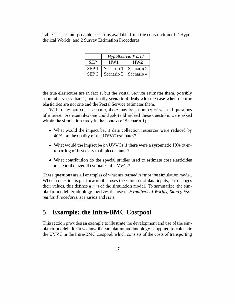
As we have described 2 HW’s and 2 SEPs, 4 scenarios are possible and aredisplayed in Table 1.
In order to draw attention to the difference between the scenarios we concen-trate for illustratory purposes on the role of mail processing; scenario one inves-tigates the case when mail processing elasticities are 1, and the Postal Serviceestimates them as 1. Scenario 2 considers what happens if mail processing elas-ticities are not one, but the Postal Service estimates them as 1, in other words thereis a systematic bias in the elasticity estimates. Scenario 3 looks at the case when
16
Table 1: The four possible scenarios available from the construction of 2 Hypo-thetical Worlds, and 2 Survey Estimation Procedures
the true elasticities are in fact 1, but the Postal Service estimates them, possiblyas numbers less than 1, and finally scenario 4 deals with the case when the trueelasticities are not one and the Postal Service estimates them.
Within any particular scenario, there may be a number of what–if questionsof interest. As examples one could ask (and indeed these questions were askedwithin the simulation study in the context of Scenario 1),
� What would the impact be, if data collection resources were reduced by40%, on the quality of the UVVC estimates?
� What would the impact be on UVVCs if there were a systematic 10% over–reporting of first class mail piece counts?
� What contribution do the special studies used to estimate cost elasticitiesmake to the overall estimates of UVVCs?
These questions are all examples of what are termedrunsof the simulation model.When a question is put forward that uses the same set of data inputs, but changestheir values, this defines arun of the simulation model. To summarize, the sim-ulation model terminology involves the use ofHypothetical Worlds, Survey Esti-mation Procedures, scenariosandruns.
5 Example: the Intra-BMC Costpool
This section provides an example to illustrate the development and use of the sim-ulation model. It shows how the simulation methodology is applied to calculatethe UVVC in the Intra-BMC costpool, which consists of the costs of transporting
17
mail between Bulk Mail Centers and mail processing facilities within their area.The Intra-BMC costpool is one of the more straight forward costpools consideredin the simulation model, but even so the presentation here is somewhat of a sim-plification of the costpool. There is always a model design decision that has tobe made concerning the level of detail to incorporate in the model. Practically,too much detail and the model may never be built, too little detail and the resultscould be misleading.
The first aspect of formulating the simulation model is to define both the Hypo-thetical World and the Survey Estimation Procedure, which specifies the method-ologies used to estimate the quantities defined in the Hypothetical World. A singleHypothetical World (HW1) and a single Survey Estimation Procedure (SEP1) arepresented in this section.
5.1 Hypothetical World construction for the Intra-BMC Cost-pool
Costs in the Hypothetical World (HW) are generated according to the log-linearcost model,
C = e�0D�1 ; (1)
where C denotes the costpool dollars, D denotes the cost driver,�1 is the elasticityof cost with respect to the driver, and�0 is a multiplicative constant that determinesthe overall level of costs.
Costpools are dollar costs associated with some activity, here, transportation.A cost driver is a measure of the activity that determines the marginal costs inthe costpool. In the Intra-BMC costpool, the costs accrue from transporting mailbetween Bulk Mail Centers, and the cost driver is cubic–foot miles. In a mailprocessing costpool, for example, the costs are employee salaries and the costdriver may be Total Pieces Handled, or Total Pieces Handled During a Peak TimePeriod. Equation (1) specifies the relationship between the total costs and the costdriver. The focus of the methods evaluated by the simulation study is to distributecosts to specific products, termed subclasses. The goal is to compute marginalcosts as a function of volume for each subclass. For theith subclass, denote thevolume (pieces) byMi. The cost driver measuring activity associated with theith
subclass in the costpool is denoted byDi, and it is assumed to be proportional tothe volume for theith subclass,
Di = �i Mi: (2)
18
The proportionality constants,�i, can vary across subclasses. The sum of theDi across all subclasses equalsD, the value of the driver. The true UVVC forsubclassi is the derivative of (1) with respect toMi. Based on the log-linear costmodel in Equation (1), and the proportional relationship between the cost driverand the volume for each subclass in (2), the UVVC is
UVVCi =dC
dMi
=C �1�i
Mi
; (3)
where�i is the distribution key share for subclass i in the Intra-BMC costpool:�i = Di=D. Note that equation 3 is comprised four components and forms thebasis for Figure 1. The formula for the UVVC does not require the explicit spec-ification of the�i. This model completes the structural specification of costs inthe HW and allows “true” UVVC’s to be calculated for each subclass. The hy-pothetical targets against which the Survey Estimation Procedure is evaluated arethe subclass UVVCs.
5.2 Survey Estimation Procedures (SEPs) for the Intra-BMCCostpool
The Survey Estimation Procedure (SEP) describes the methodological approachused to estimate the true but (supposed) unknown costs in the HW. In most of thesimulations, the UVVC formula in the SEP has the same form as the true cost-generating model. The values estimated by the SEP differ from the UVVC valuesgenerated in the HW because the SEP uses estimates of the inputs to the UVVCformula.
5.3 Data Sources for the Intra-BMC Costpool
In the Intra-BMC costpool, the estimates of the inputs to the SEP are based onfour data sources:
1. The cost value from the General Ledger account (Postal Service accountingdata).
2. The elasticity estimate from a special study.
3. The distribution key share (DKS) from the TRACS purchased transportationsampling system.
4. The volume estimates from the RPW system.
19
5.4 Assigning Input Values for a Hypothetical World for theIntra-BMC Costpool
To compute the UVVC for each subclass in the HW, values must be assigned toeach input parameter in Equation (3). There are 9 subclass volumes (8 specificsubclasses plus a category for “other”). There are also 9 subclass cubic-foot miledollar equivalents,Di, an elasticity term,�1 and the costpool dollarsC, yieldinga total of 21 input values.
The values for the input parameters are in the third column of Table 2 Thelog-linear UVVC equation (3) for the HW is solved for�0 to make the righthand side equal the allocated cost pool dollars of $251,149 thousand4. Solvingfor the parameter�0 thus insures that costs generated in the HW will equal thecost reported by the Postal Service:$251; 149 = e�0(244; 0870:9743), and thus,�0 = ln($251; 149) � 0:9743 ln(244; 087) = 0:3473. The sum of theDi isD = 244; 087.
Using the inputs in column 3 of Table 2, theUV V Ci in the HW can be calcu-lated. In this example, the calculation is only shown for the Standard B – parcelpost subclass.
The cost and elasticity values in the HW read from Table 2 are $251,149 and0.97, respectively. The distribution key share (DKS) for Standard B – parcel postsubclass is found by dividing the Standard BU parcel post subclass,Di, 71,330,by D = 244; 087 to obtain a value of 0.2922. Finally, the Standard B – parcelpost subclass volume in Table 2 is 212,828. Putting all these components into theUVVC estimating equation (3) gives a UVVC in the HW of
UVVCi =dC
dMi
=251; 149� 0:97� 0:2922
212; 828= 0:3345; (4)
so that the UVVC for Standard Parcel Post subclass from the Intra-BMC costpoolis roughly 33 cents.
5.5 Simulating Input Parameter Estimates for the Intra-BMCCostpool
Each parameter estimate input to the UVVC equations is generated according toits statistical properties determined from the analyses of the major data systemsand special studies. The statistical properties are the mean, cv, bias, sampling
4Data inputs were obtained from Postal Service FY96 values
20
distribution (e.g., Normal, Gamma etc.), and dependence on other estimates. Inthis example, the SEP estimators are assumed to have zero bias. For instance,consider the elasticity�1, which has a true value of 0.97 in the HW. The SEPvalue of�1 is generated by taking a random draw from a normal distribution witha mean of 0.97 (no bias in this input), and a cv of 1.65%. The value for the cv isbased on the Postal Service report for the Fiscal Year 1996. The SEP estimate ofthe elasticity willnot be exactly equal to the true value in the HW, but the smallerthe cv, the closer it will tend to be to the HW value (see Figure 3). Becausethe HW value and SEP estimate of the elasticity are not identical (and this is thecase for most input estimates), the SEP UVVC estimates will differ from theircorresponding HW values.
One of the key aspects of the simulation is that within any single replicationof the simulation model, all estimates of volume, revenue, etc., are generated onlyonce, and the same value is used in every costpool calculation. In this way, thecomplex dependencies and covariances inherent in the UVVC estimates across allthe costpools are implicitly accounted for by the simulation model. To simplifythe generation of the numerous parameter estimates, they are refined to a levelwhere they can be assumed statistically independent in the SEP. An example ofthe simulated (SEP) estimates of the input parameters to the UVVC estimationequation, is in the fourth column of Table 2 for a single replication (a typical runof the simulation model has 1000 replications).
Evaluating the UVVC equation with the SEP values for the Standard ParcelPost gives 37.32 cents.
In section §5.4, the UVVC equation evaluated with HW values yielded 0.3345.Thus, the simulation model has provided a target value of 33 cents for the “truth”in the HW, and a value of 37 cents for the estimate by the SEP. To evaluate the SEP,numerous replications of the SEP estimates are generated for each HW. Statisticalsummaries of the differences between the SEP estimates and the HW true valuesprovide the basis for evaluating the SEP.
6 Precision/accuracy and mean squared error
This section describes the statistical summaries used to evaluate the Survey Es-timation Procedures. They focus on the statistical properties of the differencebetween the estimated and true values of an attribute of interest, the UVVC inparticular. The difference between the estimated and true values of the attribute istheestimation error.
21
Table 2: Input Parameter Values for the HW and SEP for One Replication of theIntra-BMC Costpool
Description Input Parameter HW SEPvalues values
General Ledger Accrued dollars $251,149 $251,149Dollars (’000)
�0 0.3473 0.3473Elasticity �1 0.97 0.99
First Class Letters Flats 27,380 30,810& IPPs (incl. Presorts)Periodicals – w/n County 0 0Periodicals – Regular Rate 19,160 15,860
subclass Cost Standard – Enhanced 12,850 8,240Drivers Carrier Route(based on TRACS) Standard – Regular 46,740 48,350
Standard – Non-profit 7,930 7,650Standard – Parcel Post 71,330 81,460Standard – Library 4,010 2,970OTHER 54,690 57,720
First Class Letters Flats 93,207,952 93,302,256& IPPs (incl. Presorts)Periodicals – w/n County 877,829 888,834Periodicals – Regular Rate 6,984,301 6,995,104
subclass Volumes Standard – Enhanced 29,180,737 29,319,610in thousands Carrier Route(based on RPW) Standard – Regular 30,150,508 30,156,708
Standard – Non-profit 9,300,466 9,277,951Standard – Parcel Post 212,828 216,116Standard – Library 30,133 34,399OTHER 13,494,719 13,578,647
22
6.1 Coefficient of Variation (cv)
The coefficient of variation (cv) is a summary measure used to report uncertaintyin sample survey estimates of positive quantities. It is used to describe thesam-pling error of the estimate. There is uncertainty regarding an estimate from asurvey, because if the survey were repeated the estimate would almost certainlychange. If a census, rather than a survey were undertaken, then there would beno uncertainty in the estimate and the estimate should equal the true value. Thecv is defined as�=�, where� is the standard error of the estimate, and� its ex-pected value. The cv expresses the standard error of an estimate as a proportionof the mean value of the estimate. In practice, the numbers� and� are not knownso they are replaced by estimates from the survey. The smaller the cv, the moreprecise the estimate. In the simulation model, these summaries are calculated asfollows:
1. Each replication of the simulation provides an estimate of a subclass’ UnitVolume Variable Cost from the SEP. A simulation run with 1,000 replica-tions thus produces 1,000 such estimates.
2. After the 1,000 estimates have been computed, two summaries are derived:the mean of the 1,000 values, which is an estimate of the expected value ofthe estimator; and the standard deviation of the 1,000 values, which is anestimate of the standard error of the estimator.
3. The ratio of the standard error to the mean is then calculated to estimate thecv.
4. The cv’s are often reported on a percentage scale computed by multiplyingby 100.
The cv’s, combined with standard assumptions that lead to the approximate nor-mality of the estimate, can be used to simulate the sampling distribution of anestimator. For example, if the cv is 5%, then standard theory indicates that ap-proximately 95% of values generated from the sampling distribution are within+/- 10% of the mean of the estimator.
6.2 Bias
Bias exists when an estimate departs systematically from the parameter it is de-signed to estimate. The smaller the bias, the more accurate the estimate. For
23
example, if the true elasticity in a costpool is 0.7 and the SEP always uses anestimate of 1.0, then this estimate would bebiasedby 0.3. This situation de-scribes bias in an input parameter and is an example of anon-samplingerror.Non-sampling errors can also arise from problems such as double counting, sys-tematic mis-classification of the mail and incomplete sampling frames.
Biases in the inputs will typically lead to biases in the estimates of the outputquantities of interest as well, in particular in the UVVC estimates. In this context,a UVVC estimate would be termed biased if on average it was different from thetrue UVVC value it was attempting to estimate. For example, if the true UVVCof a product were 2c and the estimate had an average value of 3c, then this wouldconstitute a 1c, or 50% bias in the UVVC estimate. It is quite possible for allinput quantities to be unbiased but the output quantity of interest still to be biased,if these inputs are combined in a complicated (non-linear) fashion as is illustratedin Figure 1. In practice, it is the qualitative magnitude of the bias that is impor-tant, not simply the fact that bias exists. In real world sampling systems, totaleradication of all potential bias is not feasible.
Bias may also be described as a proportion of the parameter to be estimated.This facilitates comparing biases across the various subclasses of mail. When thebias is expressed as a proportion in this way, it is termedrelative bias.
6.3 Root Mean Squared Error
Root Mean Squared Error (RMSE) is an alternative way of judging the quality ofa SEP. The RMSE provides an enhancement to simply using the bias and cv asdescriptors of a SEP, because it incorporates both the cv and the bias. The MeanSquared Error (MSE) is defined as the standard error squared plus the bias squared– so that either a large standard erroror a large bias makes the MSE large. TheRMSE is the square root of the MSE, and provides a summary on the same scaleas the estimate. This means that if the cost estimates are in cents then the RMSEis measured in cents providing a directly comparable measure. RMSE providesthe foundation for comparisons between sampling and non-sampling errors. Asthe potential non-sampling error, which is revealed throughbias in the UVVCestimator, becomes larger it contributes a greater component to the RMSE.
24
7 Illustration of model results
In this section 2 sets of results are summarized from the simulation model. Thepurpose is to give an idea of the types of information that the model may provide.
7.1 UVVC cv’s, measuring sampling error
One of the main contributions to the cost estimation debate provided by the sim-ulation model, was that it represented the first time to our knowledge that uncer-tainty estimates (cv’s) have been calculated for the UVVC’s. The third columnof Table 3, under the headingSEP cv, presents these uncertainties for the 8 sub-classes incorporated in the model.
Column 1 of Table 3 indicates the subclass, column 2 contains the averagevalue of the UVVC estimate in cents. Column 3 presents the overall cv for theUVVC estimate as a percentage. Columns 4 through 9 display the cv for theUVVC, but from a run in which the variability due to a particular data systemhas been removed. For example, the change in cv forStandard A enhanced car-rier route between column 3 and column 9, where it drops from 8.00% to 1.32%shows that much of the uncertainty in this subclass arises from the Delivery Spe-cial Studies (SS). When a system’s specific cv’s have been set to zero in the modelthen we term this as “turning the system off”.5
Each of columns 4 through 9 of Table 3 shows the impact on uncertainty ofa particular data system. “ELAS” refers to elasticity data elements and “SS” tocarrier special study data elements. One conclusion is that different subclasses areimpacted differentially by the various data systems. For example, the UVVC esti-mate for Standard B parcel post realizes much of its uncertainty from the TRACSsystem. TRACS measures purchased transportation costs. This is indicated by thefact that the cv falls from 4.59 to 3.75, a drop of about 15% when the TRACSsystem is turned off. Likewise, Periodicals, within county, receives much of itsuncertainty from the IOCS system, which is due to the fact that Periodicals withincounty is a low volume subclass and thus hard to estimate from the IOCS (InOffice Cost System) sample.
In summary, Table 3 helps identify which products are most impacted bywhich data system.
5Small increases in the UVVC cv after “turning off” a system are due to simulation errors thatoccur because only 4000 replications were performed. When this occurs, it indicates that samplingand non-sampling errors from the system have a very small effect on the UVVC’s. These instancesare denoted in the table by the * symbol.
25
Table 3: Summary of the sampling variability in the UVVC estimates for the 8products used in the simulation model.
Subclass cv when a specificSubclass UVVC SEP subsystem is “turned off”
7.2 Mail processing elasticity estimates, an example where po-tential bias overwhelms sampling error
This example summarizes the potential consequences of a divergence betweenthe Hypothetical World and the SEP. In particular, the HW is taken as HW2 butthe SEP used is SEP1. That is, true elasticity values in mail processing are notequal to one, but in the SEP they assumed equal to one. In addition, the SEPover-aggregates the DKS.
The analysis reported in Table 4 reports the UVVC’s from only the Mail Pro-cessing costpools and shows that changes in elasticity estimates and DKS in MailProcessing will have a large potential impact on subclass UVVC’s. The mainconsequence of using SEP1 when HW2 represents the “truth”, is seriously biasedestimates of the UVVC’s, by between 10 to 40%.
This potential over-estimation of UVVC is due to the use of a higher elas-ticity in the SEP than the HW. Further, this potential relative bias is an order ofmagnitude larger than the cv of the UVVC estimate for all but the low volumeproducts, indicating the potential bias would be much more important than theSEP sampling variability. For example, the cv for First Class Letters Flats andIPPs is 0.82%, whereas the relative bias is 31.55%.
8 Conclusions
The simulation approach to cost estimation was shown to be a feasible methodwith which to estimate UVVCs and to evaluate the impact on these estimates ofboth the quantity of data collected and various potential sources of systematicerror. It allowed for the first time, uncertainties on subclass UVVCs to be cal-culated. Though the model was limited in its scope, covering only 8 subclassesand 29 costpools there is no fundamental reason why it could not be expanded tocapture a greater portion of the UVVC. Such an expansion would entail a sizeableeffort as the existing model took 6 months to construct. Further, if the model is toremain useful then its data inputs would have to be updated on a regular basis.
The construction of the model contributes to answering the question “how wellare costs estimated”? As such it allows one to direct both dialog and potentially,action in terms of information collection resources, to those areas of the cost gen-eration process that are most influential on the costs themselves. The model hasthe potential to be the foundation of a methodology that would provide a rationalallocation of information collection resources. However, if it were to take on this
27
Table 4: UVVC Estimates and cv’s of UVVC’s in the Mail Processing costpoolswhen the Hypothetical World is HW2 but the SEP is SEP1
First Class 5.42 7.13 31.55 0.82Letters Flats& IPPsPeriodicals 1.52 1.87 22.37 14.12within countyPeriodicals 5.83 6.58 12.86 2.05regular rateStandard A 0.80 0.91 12.50 2.60enhancedcarrier routeStandard A 4.51 5.59 23.95 1.40regular rateStandard A 3.48 4.36 25.29 2.12non-profitStandard B 64.98 82.78 26.45 3.38parcel postStandard B 47.07 67.84 44.13 13.31library
28
role then additional information would need to be incorporated, in particular thecosts of collecting information.
Though the model was constructed within the context of the Data QualityStudy there is no reason why the results from the model could not be used ina wider context than the Postal rate setting environment alone. The underlyingquestions that motivated the construction of the model, that is the quality of theraw material to an information based decision system, could be posed to any in-formation system, and in particular could include operating data systems.
As a final point, there is nothing intrinsic to the simulation methodology thatwould prohibit its use outside of the Postal Service environment. Other industriesmay find benefit in taking a hard look, and attempting to quantify the qualityof their data. As management decisions are increasingly information driven, theremust come a point when the quality of the raw material inputs to those informationsystems becomes paramount. The approach taken here may provide a frameworkfrom which to formulate data quality metrics in a wider context.
In summary, if it is critically important to measure cost, then one should wantto know how well those costs have been measured. The simulation model is a firststep in this endeavor.
29
References
M.D. Bradley, J.L. Colvin, and M.A. Smith. Measuring product costs for ratemak-ing: The United States Postal Service. In M. A. Crew and P. R. Kleindorfer,editors,Regulation and the Nature of Postal and Delivery Services. KluwerAcademic Publishers, Boston, MA, 1993.
R. Cooper and R.S. Kaplan.The Design of Cost Management Systems. PrenticeHall, Englewood Cliffs, NJ, 1991.
M.A. Crew and P.R. Kleindorfer.The Economics of Postal Service. Kluwer Aca-demic Publishers, Boston, MA, 1992.
T.M. Ezzati-Rice, W. Johnson, M. Khare, R.J.A. Little, J.L. Schafer, and D.B.Rubin. A simulation study to evaluate the performance of multiple imputationin the NCHS Health Exam Survey. InProceedings of the Bureau of the Census.11th Annual Research Conference, pages 257–266, 1995.
LINX. Data Quality Study, April 1999. Available online athttp://www.usps.gov/clr/dqs.htm.
T.E. Raghunathan and D.B. Rubin. Roles for Bayesian techniques in survey sam-pling. In Proceedings of the Survey Methodology Section of the Statistical So-ciety of Canada, pages 51–55, 1997.