HAL Id: hal-00728587 https://hal.archives-ouvertes.fr/hal-00728587 Submitted on 30 Aug 2012 HAL is a multi-disciplinary open access archive for the deposit and dissemination of sci- entific research documents, whether they are pub- lished or not. The documents may come from teaching and research institutions in France or abroad, or from public or private research centers. L’archive ouverte pluridisciplinaire HAL, est destinée au dépôt et à la diffusion de documents scientifiques de niveau recherche, publiés ou non, émanant des établissements d’enseignement et de recherche français ou étrangers, des laboratoires publics ou privés. Simulation of a UAV ground control station Alain Ajami, Thibault Maillot, Nicolas Boizot, Jean-François Balmat, Jean-Paul Gauthier To cite this version: Alain Ajami, Thibault Maillot, Nicolas Boizot, Jean-François Balmat, Jean-Paul Gauthier. Simulation of a UAV ground control station. 9th International Conference on Modeling, Optimization SIMulation, Jun 2012, Bordeaux, France. 2012. <hal-00728587>
Transcript
HAL Id: hal-00728587https://hal.archives-ouvertes.fr/hal-00728587
Submitted on 30 Aug 2012
HAL is a multi-disciplinary open accessarchive for the deposit and dissemination of sci-entific research documents, whether they are pub-lished or not. The documents may come fromteaching and research institutions in France orabroad, or from public or private research centers.
L’archive ouverte pluridisciplinaire HAL, estdestinée au dépôt et à la diffusion de documentsscientifiques de niveau recherche, publiés ou non,émanant des établissements d’enseignement et derecherche français ou étrangers, des laboratoirespublics ou privés.
Simulation of a UAV ground control stationAlain Ajami, Thibault Maillot, Nicolas Boizot, Jean-François Balmat,
Jean-Paul Gauthier
To cite this version:Alain Ajami, Thibault Maillot, Nicolas Boizot, Jean-François Balmat, Jean-Paul Gauthier. Simulationof a UAV ground control station. 9th International Conference on Modeling, Optimization
SIMulation, Jun 2012, Bordeaux, France. 2012. <hal-00728587>
ABSTRACT: In this article we present the development of a UAV ground control station simulator. Wepropose a module based description of the architecture of this simulator. We recall the nonlinear model of afixed-wing aircraft. Finally, we outline ideas for improved path planning tasks. The approach is made clearthrough several diagrams, figures of the resulting station are displayed.
KEYWORDS: path planning, simulation, UAV, optimal control, inverse optimal control problem
1 INTRODUCTION
Today’s interest in drone technology led to an in-creasing number of dedicated projects (Tisdale, Kim& Hedric 2009, Kim, Shim & Sastry 2002, Fabiani,Fuertes, Piquereau, Mampey & Teichteil-Konigsbuch2007, Ippolito, Yeh & Campbell 2009). Thoseprojects tackle problems such as the autonomy im-provement, the reduction of drone crashes due to pooravailability of information, the organization of droneswarms, or the calculation of secure and optimal flightpaths. LSIS laboratory joins this research effort in theframework of project SHARE. Supported by a con-sortium of companies and research laboratories1, theresearch aims to develop a universal and interopera-ble ground control station for fixed and rotary-wingUAVs for a reduced number of operators. Specifi-cally, LSIS focuses on the connections between theUAV trajectory and its sensors. As a consequence,improved path planning algorithms that take into ac-count payload requirements, optimal costs and obsta-cles (or no flight zones) avoidance are needed.
In order to test and demonstrate our techniques aground control station simulator is required. The useof engineering and simulation softwares allows shorterdevelopment time and still maintain portability of thecode. Since the development is done in close contactwith our research partners, modularity is a key fac-tor. Indeed, we want to be able to easily add, remove,or modify parts of the simulator. Another challenge
is to determine the automation level of the station.(Cummings, Platts & Sulmistras 2006, Sheridan, Ver-plank & Brooks 1978) propose insights on automa-tion strategies that are useful to describe the simu-lator. On the Sheridan-Verplank scale, the stationranks no more than 3 and, according to (Cummingset al. 2006), it has a level of interoperability of 4 withrespect to the STANAG 4586 classification. This lat-ter level can be described as follows: the ground sta-tion allows the control and monitoring of the UAV atthe exception of launch and recovery situations. Thesimulation of such a device starts with the simulationof the aircraft’s trajectory. Then follows the emula-tion of all the data exchanged between the operatorand the UAV through the station, and finally of thecontrol algorithms.
Classic tools for the implementation of the aircraft’sdynamics, the controller part and the man machineinterface are Matlab and Matlab/Simulink. We pref-ered the use of S-functions to a systematic blockbased implementation in order to ease portability incase of discard of Matlab’s automatic code genera-tion features. The simulation of the virtual envi-ronment and of the video flow is done by means ofby a flight simulator (Craighead, Murphy, Burke &Goldiez 2007). Flightgear which is open source andinterfaces nicely with Matlab/Simulink is used (Yang,Qi & Shan 2009, Sorton & Hammaker 2005).
The rest of this article is organised as follows. Thestructure of the simulator is presented in section 2.It is broken into several modules which functionalitiesare explained. The nonlinear aircraft dynamics are re-called in section 3. Although project SHARE aims ata ground control station that addresses both fixed and
MOSIM’12 - June 06-08, 2012 - Bordeaux - France
rotative wing aircrafts, we focus on fixed-wing ones.Finally section 4 contains both low and high level de-scriptions of the control module (cf. figure 4). Inparticular, several notions regarding high level pathplanning and learning algorithms are sketched in sub-section 4.2.
2 SIMULATOR
A ground control station simulation instance has twomain parts: the initialization phase and the scenariorealization. The initialization phase allows the defi-nition of the parameters that are specific to a givensimulation instance, this step is detailed in subsec-tion 2.1. During the simulation several different mis-sions can be realized accordingly to the operator’sscenario. The architecture of this scenario realizationpart is detailed in subsection 2.2.
2.1 Simulator’s Initialization Phase
We divide simulation parameters into two categories:setup parameters and core parameters. Core param-eters contribute to the simulation inner mechanisms:model parameters (subsections 3.3.1, 3.3.2 and 3.4)and control parameters (section 4). As such the usercannot manipulate them directly: they are eitherloaded through a setup assistant utility or managedthrough a modify/create assistant.
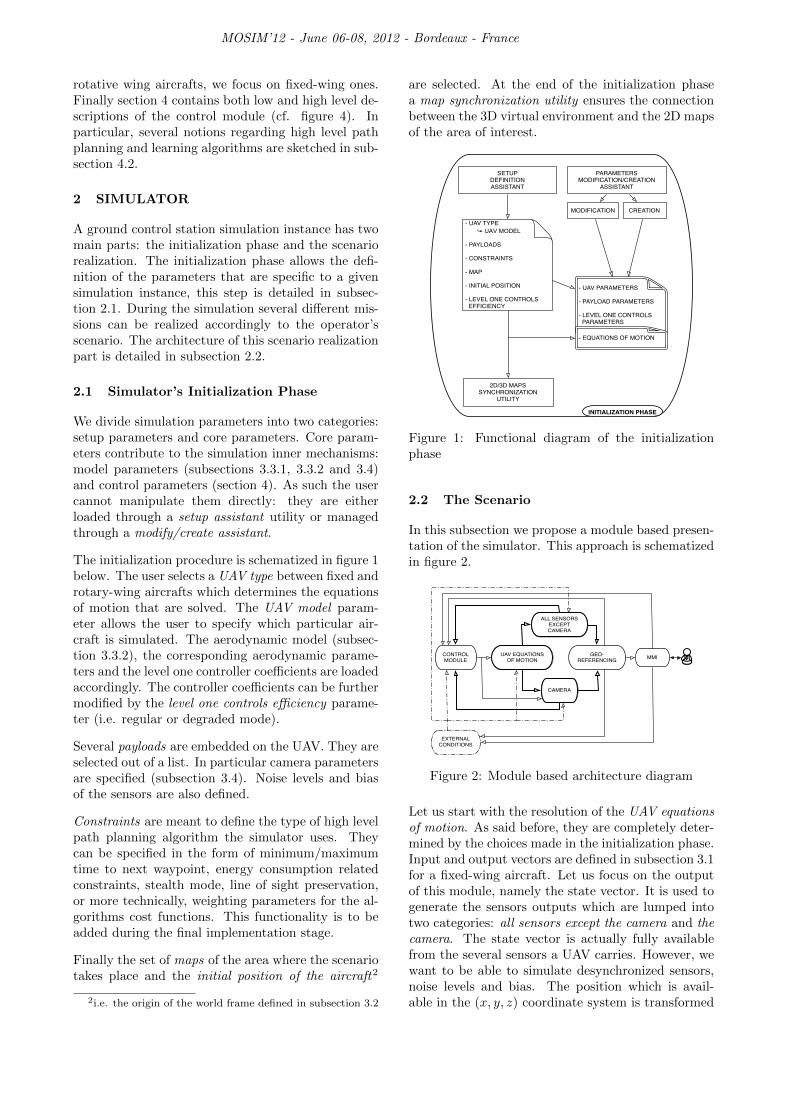
The initialization procedure is schematized in figure 1below. The user selects a UAV type between fixed androtary-wing aircrafts which determines the equationsof motion that are solved. The UAV model param-eter allows the user to specify which particular air-craft is simulated. The aerodynamic model (subsec-tion 3.3.2), the corresponding aerodynamic parame-ters and the level one controller coefficients are loadedaccordingly. The controller coefficients can be furthermodified by the level one controls efficiency parame-ter (i.e. regular or degraded mode).
Several payloads are embedded on the UAV. They areselected out of a list. In particular camera parametersare specified (subsection 3.4). Noise levels and biasof the sensors are also defined.
Constraints are meant to define the type of high levelpath planning algorithm the simulator uses. Theycan be specified in the form of minimum/maximumtime to next waypoint, energy consumption relatedconstraints, stealth mode, line of sight preservation,or more technically, weighting parameters for the al-gorithms cost functions. This functionality is to beadded during the final implementation stage.
Finally the set of maps of the area where the scenariotakes place and the initial position of the aircraft2
2i.e. the origin of the world frame defined in subsection 3.2
are selected. At the end of the initialization phasea map synchronization utility ensures the connectionbetween the 3D virtual environment and the 2D mapsof the area of interest.
SETUP DEFINITIONASSISTANT
- UAV TYPE ➥ UAV MODEL
- PAYLOADS
- CONSTRAINTS
- MAP
- INITIAL POSITION
- LEVEL ONE CONTROLS EFFICIENCY
PARAMETERS MODIFICATION/CREATION
ASSISTANT
MODIFICATION CREATION
2D/3D MAPS SYNCHRONIZATION
UTILITY
- UAV PARAMETERS
- PAYLOAD PARAMETERS
- LEVEL ONE CONTROLS PARAMETERS
- EQUATIONS OF MOTION
INITIALIZATION PHASE
Figure 1: Functional diagram of the initializationphase
2.2 The Scenario
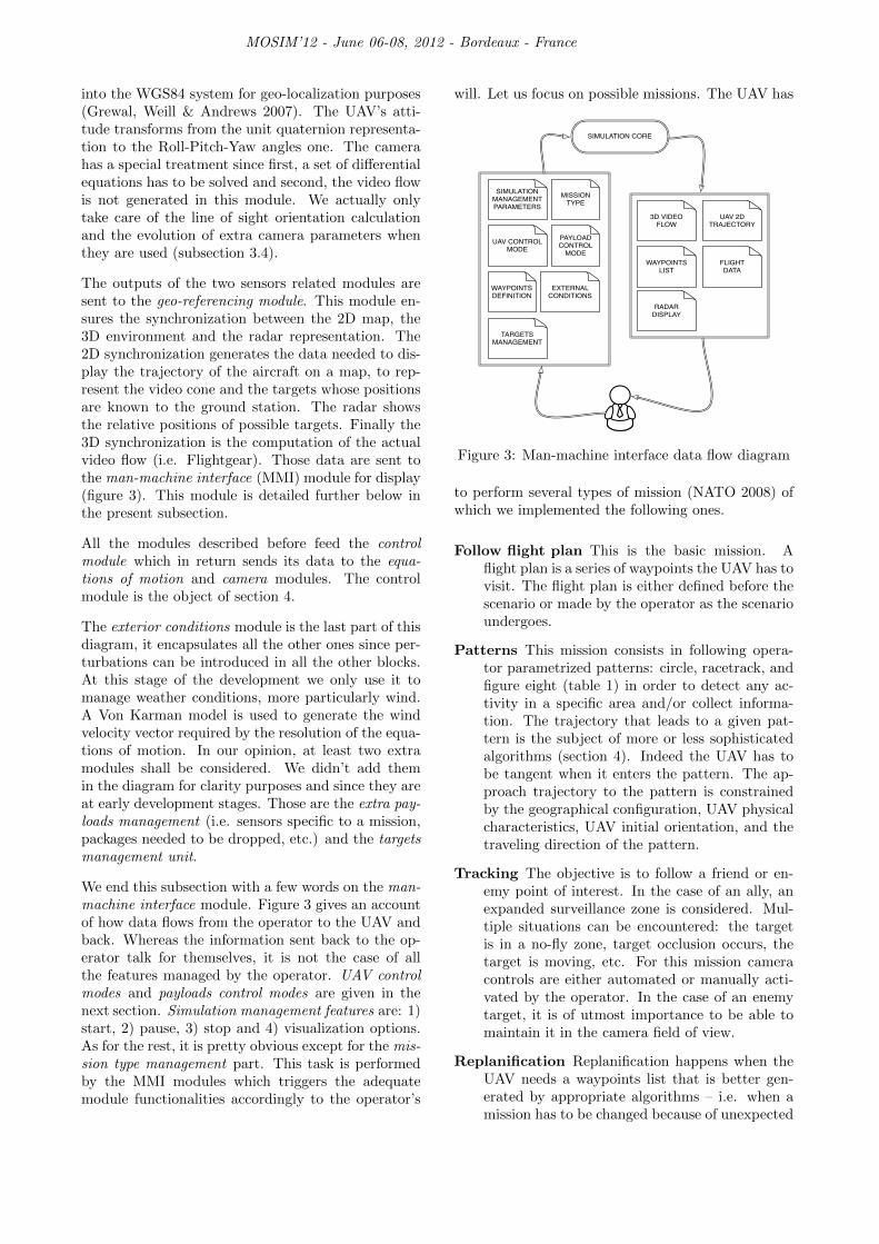
In this subsection we propose a module based presen-tation of the simulator. This approach is schematizedin figure 2.
UAV EQUATIONSOF MOTION
ALL SENSORS EXCEPT CAMERA
CAMERA
CONTROLMODULE
GEO-REFERENCING MMI
EXTERNALCONDITIONS
Figure 2: Module based architecture diagram
Let us start with the resolution of the UAV equationsof motion. As said before, they are completely deter-mined by the choices made in the initialization phase.Input and output vectors are defined in subsection 3.1for a fixed-wing aircraft. Let us focus on the outputof this module, namely the state vector. It is used togenerate the sensors outputs which are lumped intotwo categories: all sensors except the camera and thecamera. The state vector is actually fully availablefrom the several sensors a UAV carries. However, wewant to be able to simulate desynchronized sensors,noise levels and bias. The position which is avail-able in the (x, y, z) coordinate system is transformed
MOSIM’12 - June 06-08, 2012 - Bordeaux - France
into the WGS84 system for geo-localization purposes(Grewal, Weill & Andrews 2007). The UAV’s atti-tude transforms from the unit quaternion representa-tion to the Roll-Pitch-Yaw angles one. The camerahas a special treatment since first, a set of differentialequations has to be solved and second, the video flowis not generated in this module. We actually onlytake care of the line of sight orientation calculationand the evolution of extra camera parameters whenthey are used (subsection 3.4).
The outputs of the two sensors related modules aresent to the geo-referencing module. This module en-sures the synchronization between the 2D map, the3D environment and the radar representation. The2D synchronization generates the data needed to dis-play the trajectory of the aircraft on a map, to rep-resent the video cone and the targets whose positionsare known to the ground station. The radar showsthe relative positions of possible targets. Finally the3D synchronization is the computation of the actualvideo flow (i.e. Flightgear). Those data are sent tothe man-machine interface (MMI) module for display(figure 3). This module is detailed further below inthe present subsection.
All the modules described before feed the controlmodule which in return sends its data to the equa-tions of motion and camera modules. The controlmodule is the object of section 4.
The exterior conditions module is the last part of thisdiagram, it encapsulates all the other ones since per-turbations can be introduced in all the other blocks.At this stage of the development we only use it tomanage weather conditions, more particularly wind.A Von Karman model is used to generate the windvelocity vector required by the resolution of the equa-tions of motion. In our opinion, at least two extramodules shall be considered. We didn’t add themin the diagram for clarity purposes and since they areat early development stages. Those are the extra pay-loads management (i.e. sensors specific to a mission,packages needed to be dropped, etc.) and the targetsmanagement unit.
We end this subsection with a few words on the man-machine interface module. Figure 3 gives an accountof how data flows from the operator to the UAV andback. Whereas the information sent back to the op-erator talk for themselves, it is not the case of allthe features managed by the operator. UAV controlmodes and payloads control modes are given in thenext section. Simulation management features are: 1)start, 2) pause, 3) stop and 4) visualization options.As for the rest, it is pretty obvious except for the mis-sion type management part. This task is performedby the MMI modules which triggers the adequatemodule functionalities accordingly to the operator’s
will. Let us focus on possible missions. The UAV has
UAV CONTROLMODE
MISSIONTYPE
SIMULATIONMANAGEMENTPARAMETERS
EXTERNAL CONDITIONS
WAYPOINTSDEFINITION
PAYLOADCONTROL
MODE
TARGETSMANAGEMENT
3D VIDEOFLOW
UAV 2D TRAJECTORY
WAYPOINTSLIST
FLIGHT DATA
RADARDISPLAY
SIMULATION CORE
Figure 3: Man-machine interface data flow diagram
to perform several types of mission (NATO 2008) ofwhich we implemented the following ones.
Follow flight plan This is the basic mission. Aflight plan is a series of waypoints the UAV has tovisit. The flight plan is either defined before thescenario or made by the operator as the scenarioundergoes.
Patterns This mission consists in following opera-tor parametrized patterns: circle, racetrack, andfigure eight (table 1) in order to detect any ac-tivity in a specific area and/or collect informa-tion. The trajectory that leads to a given pat-tern is the subject of more or less sophisticatedalgorithms (section 4). Indeed the UAV has tobe tangent when it enters the pattern. The ap-proach trajectory to the pattern is constrainedby the geographical configuration, UAV physicalcharacteristics, UAV initial orientation, and thetraveling direction of the pattern.
Tracking The objective is to follow a friend or en-emy point of interest. In the case of an ally, anexpanded surveillance zone is considered. Mul-tiple situations can be encountered: the targetis in a no-fly zone, target occlusion occurs, thetarget is moving, etc. For this mission cameracontrols are either automated or manually acti-vated by the operator. In the case of an enemytarget, it is of utmost importance to be able tomaintain it in the camera field of view.
Replanification Replanification happens when theUAV needs a waypoints list that is better gen-erated by appropriate algorithms – i.e. when amission has to be changed because of unexpected
MOSIM’12 - June 06-08, 2012 - Bordeaux - France
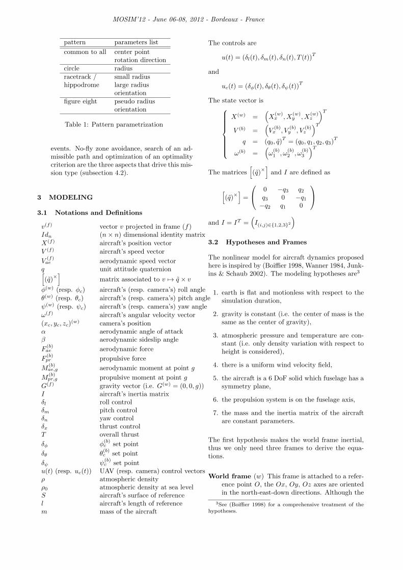
pattern parameters list
common to all center pointrotation direction
circle radiusracetrack / small radiushippodrome large radius
orientationfigure eight pseudo radius
orientation
Table 1: Pattern parametrization
events. No-fly zone avoidance, search of an ad-missible path and optimization of an optimalitycriterion are the three aspects that drive this mis-sion type (subsection 4.2).
3 MODELING
3.1 Notations and Definitions
v(f) vector v projected in frame (f)Idn (n× n) dimensional identity matrixX(f) aircraft’s position vectorV (f) aircraft’s speed vector
V(f)ae aerodynamic speed vectorq unit attitude quaternion[(q)×]
u(t) (resp. uc(t)) UAV (resp. camera) control vectorsρ atmospheric densityρ0 atmospheric density at sea levelS aircraft’s surface of referencel aircraft’s length of referencem mass of the aircraft
The controls are
u(t) = (δl(t), δm(t), δn(t), T (t))T
and
uc(t) = (δφ(t), δθ(t), δψ(t))T
The state vector is
X(w) =(X
(w)x , X
(w)y , X
(w)z
)TV (b) =
(V
(b)x , V
(b)y , V
(b)z
)Tq = (q0, q)
T= (q0, q1, q2, q3)
T
ω(b) =(ω(b)1 , ω
(b)2 , ω
(b)3
)TThe matrices
[(q)×]
and I are defined as
[(q)×]
=
0 −q3 q2q3 0 −q1−q2 q1 0
and I = IT =
(I(i,j)∈{1,2,3}2
)3.2 Hypotheses and Frames
The nonlinear model for aircraft dynamics proposedhere is inspired by (Boiffier 1998, Wanner 1984, Junk-ins & Schaub 2002). The modeling hypotheses are3
1. earth is flat and motionless with respect to thesimulation duration,
2. gravity is constant (i.e. the center of mass is thesame as the center of gravity),
3. atmospheric pressure and temperature are con-stant (i.e. only density variation with respect toheight is considered),
4. there is a uniform wind velocity field,
5. the aircraft is a 6 DoF solid which fuselage has asymmetry plane,
6. the propulsion system is on the fuselage axis,
7. the mass and the inertia matrix of the aircraftare constant parameters.
The first hypothesis makes the world frame inertial,thus we only need three frames to derive the equa-tions.
World frame (w) This frame is attached to a refer-ence point O, the Ox, Oy, Oz axes are orientedin the north-east-down directions. Although the
3See (Boiffier 1998) for a comprehensive treatment of thehypotheses.
MOSIM’12 - June 06-08, 2012 - Bordeaux - France
aircraft’s position expressed through the equa-tions of motion is given in the (x, y, z) system, weneed to express it in the WGS84 system in orderto perform geo-referencing (Grewal et al. 2007).
Body frame (b) This frame is attached to the air-craft’s center of mass (G). The Gx(b) axis goesalong the fuselage axis. The Gz(b) axis is taken inthe plane of symmetry of the aircraft and pointsdownward, and Oy(b) = Oz(b) ×Ox(b)The composition of a translation and a rotationtransforms frame (w) into frame (b). The rota-tion defines the attitude of the aircraft. We usethe Euler angles Roll-Pitch-Yaw parametrizationfor its physical meaning, and the unit quater-nion parametrization to solve differential equa-tions (Junkins & Schaub 2002, Diebel 2006).
Aerodynamic frame (a) This frame shares his ori-gin with frame (b). The Gx(a) axis is carried bythe aerodynamic velocity vector. The rotationthat transforms Gx(b) into Gx(a) is parametrizedby the angle of attack and the sideslip angle.The other axes are obtained through this rota-tion (subsection 3.3.2).
3.3 Aircraft Dynamics
3.3.1 Equations of Motion
The dynamic resultant theorem and the dynamic mo-ment theorem write as
m ddt V
(b) = F (b)ae + F (b)
pr +mG(b) − ω(b) ×mV (b)
(1)
Iω(b) = M (b)ae,g +M (b)
pr,g − ω(b) × Iω(b) (2)
where
F (b)ae =
ρSV 2ae
2
−C(b)A
C(b)Y
−C(b)N
F (b)pr =
F(b)pr,x
F(b)pr,y
F(b)pr,z
(3)
M (b)ae =
ρSlV 2ae
2
ClCmCn
M (b)pr =
M(b)x
M(b)y
M(b)z
(4)
The rotation matrix from the world frame to the bodyframe expressed in terms of q, and the dynamics of qare (Junkins & Schaub 2002)
R(q) =(q20 − qqT
)Id3 + 2
(qT q − q0
[q×])
(5)
and
q =1
2
(0 −ω(b)
ω(b) −[(ω(b)
)×] ) q (6)
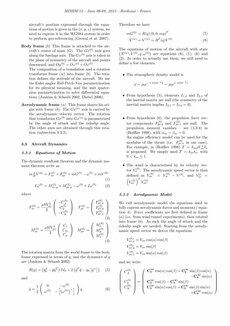
Therefore we have
mG(b) = R(q) (0, 0,mg)T
(7)
X(w) = V (w) = RT (q)V (b) (8)
The equations of motion of the aircraft with state(X(w), V (b), q, ω(b)
)are equations (8), (1), (6) and
(2). In order to actually use them, we still need todefine a few elements.
• The atmospheric density model is
ρ = ρ0e−1.1210−4h = ρ0e
1.1210−4z
• From hypothesis (5), elements I1,2 and I2,3 ofthe inertial matrix are null (the symmetry of theinertial matrix implies I2,1 = I3,2 = 0).
• From hypothesis (6), the propulsion force vec-
tor components F(b)pr,y and F
(b)pr,z are null. The
propulsion moment vanishes – see (4.3.4) in(Boiffier 1998), with αm = βm = 0.An engine efficiency model can be used for the
modulus of the thrust (i.e. F(b)pr,x in our case).
For example, in (Boiffier 1998) T = kmρVλaeδx
is proposed. We simply used T = kmδx, with0 < km ≤ 1.
• The wind is characterized by its velocity vec-
tor V(b)w . The aerodynamic speed vector is then
defined as V(b)ae = V
(b)w − V (b), and V 2
ae =(V
(b)ae
)TV
(b)ae
3.3.2 Aerodynamic Model
We call aerodynamic model the equations used tofully express aerodynamic forces and moments ( equa-tion 4). Force coefficients are first defined in frame(a) (i.e. from wind tunnel experiments), then rotatedinto frame (b). As such the angle of attack and thesideslip angle are needed. Starting from the aerody-namic speed vector we derive the equations
V (b)ae,x = Vae cos(α) cos(β)
V (b)ae,y = Vae sin(β)
V (b)ae,z = Vae sin(α) cos(β)
and we writeC
(b)A
C(b)Y
C(b)N
=
C
(a)x cos(α) cos(β) + C
(a)y sin(β) cos(α)
−C(a)z sin(α)
C(a)y cos(β)−C
(a)x sin(β)
C(a)x sin(α) cos(β) + C
(a)y sin(β) sin(α)
+C(a)z cos(α)
MOSIM’12 - June 06-08, 2012 - Bordeaux - France
There are many possible models for C(a)x , C
(a)y , C
(a)z ,
Cl, Cm and Cn (Wanner 1984, Schmidt 1998). Wecite the simple model
C(a)x = Cx,0 + kiC
2z
C(a)y = Cy,ββ + Cy,δnδn
C(a)z = Cz,αα+ Cz,δmδm
Cl = Cl,β sin(β) + l(Cl,ω1
ω1
Vae+ Cl,ω3
ω3
Vae
)+Cl,δlδl + Cl,δnδl
Cm = Cm,α + Cm,δmδm + Cm,ω2
lω2
Vae
Cn = Cn,β + Cn,δnδn + Cn,ω3
ω3
Vae
3.4 Camera Dynamics
This model tracks the orientation of the line of sightof the camera. This latter is assumed to be solidlyattached to the center of mass of the aircraft:
xwc = X(w)x
ywc = X(w)y
zwc = X(w)z
Following camera datasheet specifications (wescam2011), the dynamics can be approximated as a firstorder response to an attitude set point. This atti-
tude set point is given in the (b) frame (i.e. φ(b)c =
(−φ(b)c + φ(b)set)/τ). The time constant τ defines the
speed of the camera steering system. Constraints onthe coverage can be expressed in terms of constraintson the inputs rather than on the output (a significantasset both for implementation and optimal controlpurposes).
φ(w)c = ω
(b)1 − 1
τ
(φ(w)c − φ(w)
)+ 1
τ δφ
θ(w)c = ω
(b)2 − 1
τ
(θ(w)c − θ(w)
)+ 1
τ δθ
ψ(w)c = ω
(b)3 − 1
τ
(ψ(w)c − ψ(w)
)+ 1
τ δψ
(9)
Extra parameters that can be used to model thecamera system are described in the following table(wescam 2011).
parameter indicative value
optical eye field of view 36 to 1 (◦)IR fields of view 30, 7 and 1.8 (◦)frequency 24 (FPS)turret coverageazimuth 0 to 360 (◦)elevation 90 to -120(◦)roll na
turret steering speed 0 to 60 (◦/sec)turret stabilization quality abt 3.10−3 (◦)autofocus time constant 0
(i.e. instantaneous)
4 CONTROL MODULE
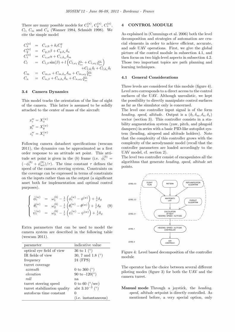
As explained in (Cummings et al. 2006) both the leveldecomposition and strategies of automation are cru-cial elements in order to achieve efficient, accurate,and safe UAV operations. First, we give the globalpicture of the control module in subsection 4.1, andthen focus on two high-level aspects in subsection 4.2.Those two important topics are path planning andlearning techniques.
4.1 General Considerations
Three levels are considered for this module (figure 4).Level zero corresponds to a direct access to the controlsurfaces of the UAV. Although unrealistic, we keptthe possibility to directly manipulate control surfacesas far as the simulator only is concerned.The level one controller input signal is of the formheading, speed, altitude. Output is a (δl, δm, δn, δx)vector (section 3). This controller consists in a sta-bility augmentation system (yaw, pitch, and phugoiddampers) in series with a basic PID-like autopilot sys-tem (heading, airspeed and altitude holders). Notethat the complexity of this controller grows with thecomplexity of the aerodynamic model (recall that thecontroller parameters are loaded accordingly to theUAV model, cf. section 2).The level two controller consist of encapsulates all thealgorithms that generate heading, speed, altitude setpoints.
REPLANIFICATIONALGORITHMPATTERNFLIGHT
PLAN
WAYPOINTSLIST
CALCULATIONOF NEXT
HEADING / SPEED / ALTITUDE
PURSUITALGORITHM
HEADING / SPEED / ALTITUDECONTROLLER
UAVCONTROLSLEVEL 0
LEVEL 1
LEVEL 2.1
LEVEL 2.2
LEVEL 2.3
Figure 4: Level based decomposition of the controllermodule
The operator has the choice between several differentpiloting modes (figure 3) for both the UAV and thecamera turret.
Manual mode Through a joystick, the heading,speed, altitude setpoint is directly controlled. Asmentioned before, a very special option, only
MOSIM’12 - June 06-08, 2012 - Bordeaux - France
available in simulation, grants access to the con-trol surfaces of the UAV.
Semi-manual mode At least one of the three com-ponents of the heading, speed, altitude setpointis managed by the system – e.g. altitude is keptfixed.
Automatic mode The level one set point is definedby a level two algorithm which depends on theactive mission.
The control modes of the camera are simpler to han-dle as only manual and automatic modes are pro-posed. Knowing the lastly visited, the targeted andthe next on the list waypoints, the calculation ofthe new heading, speed, altitude set point is easilyobtained from geometry. Note that a waypoint isdefined by its WGS84 coordinates and an optionaltimestamp. When minimum/maximum time betweenwaypoints constraints are activated, timestamps areused to adjust the set speed.
The next three parts to explain are the pattern, re-planification and pursuit algorithms. As said before apattern is defined by a set of parameters (table 1) assuch a waypoints list describes it. What remains to bedone is to propose a trajectory that allows the UAVto reach the pattern with the correct configuration(i.e. tangentially), starting from any initial point andany initial orientation. This is one of the jobs doneby the replanification algorithm. The second one isto generate optimal trajectory to travel through anarea without having a pre-established flight plan. Astrategy in order to use this algorithm is to solve a re-planification problem, then propose the solution tra-jectory as a list of waypoints and finally refresh thelist through a new calculation each time a waypoint isreached. The pursuit algorithm output can be seen asa heading, altitude, speed vector that is recomputedwhenever necessary.
A few insights on replanification algorithms are pro-posed in the next subsection. We even make one stepfarther by presenting experiment based learning ofoptimal cost functions.
4.2 planning and Learning
4.2.1 Introduction
In the context of the project SHARE we have also toachieve two extra tasks:
1. Fill in the modules called replanification algo-rithm and pursuit algorithm in figure 4. Thereis a lot of bibliography on this topic (Betts 2001,Bullo & Lewis 2004, Fliess, Levine, Martin &Rouchon 1995, Kim et al. 2002, Laumond 1998,
LaValle 2006, Park, Deyst & How 2004, Van-Nieuwstadt & Murray 1998) , non exhaustively.These classical algorithms are based upon verydifferent approaches such as geometric control,optimal control, flatness. In fact we are also de-veloping our own methods that we present brieflybelow (subsection 4.2.2).
2. An idea to develop planification/replanificationmethods is to learn from the behavior of ex-perimented pilots. We do this here for HALE(High Altitude Long Endurance) drones. Insubsection 4.2.3 we present briefly our ideas,that are inspired from the beautiful work ofJean and al. in the papers (Chitour, Jean &Mason 2012, Chittaro, Jean & Mason to ap-pear). In these papers, they attack the prob-lem of identification of the cost minimized in hu-man locomotion. Our problem is very similarsince HALE drones behave kinematically more orless as a human being moving on a plane (con-stant altitude, constant speed). There is a lotof other methods dedicated to this human loco-motion problem, see for instance (Li, Todorov &Liu 2011, Berret, Darlot, Jean, Pozzo, Papaxan-this & Gauthier 2008).
4.2.2 Planification/Replanification
In general the mission of a drone is planed in advanceand specified by a certain number of checkpoints anda certain number of patterns (line, circle, figure eightand hippodrome). There is the need of on-line replan-ification methods when the mission is interrupted andthe drone has to:
• Join a fixed target and turn around following acertain pattern,
• Join a moving target and follow it. This is notan obvious problem when the minimum speed ofthe drone is higher than the target speed.
Regarding the case (not yet treated above) of HALErotorcraft-based drones, they behave kinematicallymore or less as the classical “simple car” model(Laumond 1998). Hence one can formulate an opti-mal control problem which looks like a left-invariantsubriemannian problem over the group of motions ofthe plane. On this topic there is the beautiful com-plete mathematical work of Yuri Sachkov (Moiseev& Sachkov 2010, Sachkov 2010, Sachkov 2011) thatdoes the job, if no obstacles are taken into account. Ifobstacles occur, the Sachkov method can be coupledto a method for finding first non admissible trajec-tories avoiding obstacles and approximating them bypieces from the Sachkov synthesis. Several methodsare available to find such non admissible trajectories,
MOSIM’12 - June 06-08, 2012 - Bordeaux - France
see (LaValle 2006) for an extensive overview of suchtechniques.
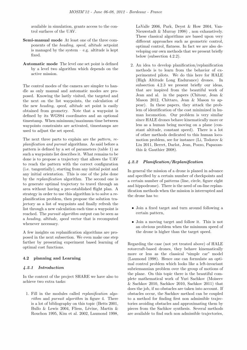
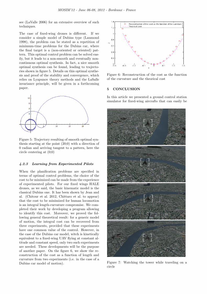
The case of fixed-wing drones is different. If weconsider a simple model of Dubins type (Laumond1998), the problem can be stated as a repetition ofminimum-time problems for the Dubins car, wherethe final target is a (non-oriented or oriented) pat-tern. This optimal control problem can be solved eas-ily, but it leads to a non-smooth and eventually non-continuous optimal synthesis. In fact, a nice smoothoptimal synthesis can be found, leading to trajecto-ries shown in figure 5. Details on this optimal synthe-sis and proof of the stability and convergence, whichrelies on Lyapunov theory methods and the LaSalleinvariance principle, will be given in a forthcomingpaper.
Figure 5: Trajectory resulting of smooth optimal syn-thesis starting at the point (20;0) with a direction of0 radian and arriving tangent to a pattern, here thecircle centering at (0;0)
4.2.3 Learning from Experimented Pilots
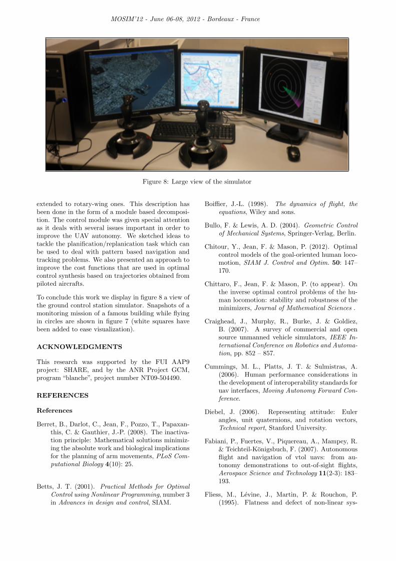
When the planification problems are specified interms of optimal control problems, the choice of thecost to be minimized can be made from the experienceof experimented pilots. For our fixed wings HALEdrones, as we said, the basic kinematic model is theclassical Dubins one. It has been shown by Jean andal. (Chitour et al. 2012, Chittaro et al. to appear)that the cost to be minimized for human locomotionis an integral length-curvature compromise. We com-pleted their work by developing a program allowingto identify this cost. Moreover, we proved the fol-lowing general theoretical result: for a generic modelof motion, the integral cost can be recovered fromthree experiments, provided that these experimentshave one common value of the control. However, inthe case of the Dubins car model, witch is kineticallyequivalent to a fixed-wing UAV flying at constant al-titude and constant speed, only two such experimentsare needed. These developments will be the purposeof another paper. On the figure 6, we show the re-construction of the cost as a function of length andcurvature from two experiments (i.e. in the case of aDubins car model of motion).
Figure 6: Reconstruction of the cost as the functionof the curvature and the theorical cost
5 CONCLUSION
In this article we presented a ground control stationsimulator for fixed-wing aircrafts that can easily be
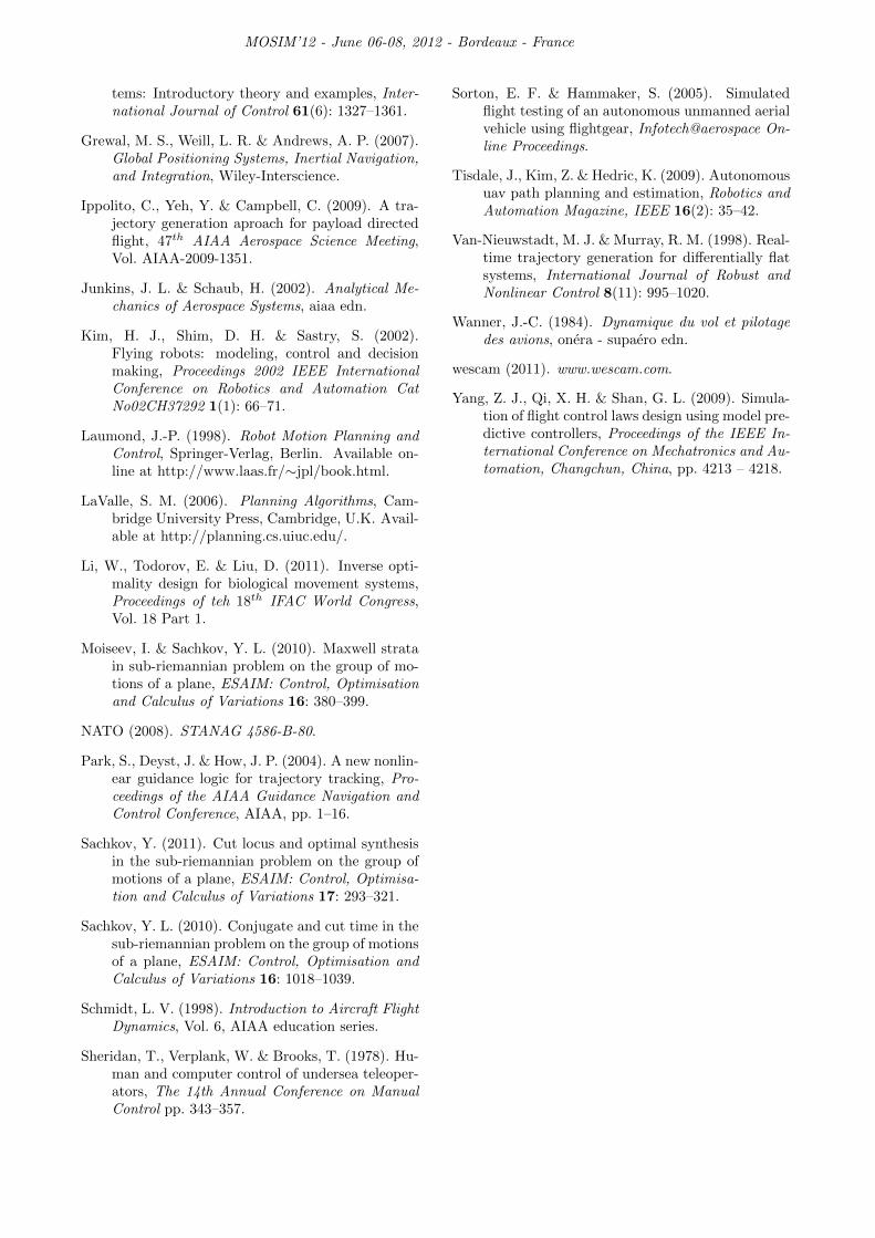
Figure 7: Watching the tower while traveling on acircle
MOSIM’12 - June 06-08, 2012 - Bordeaux - France
Figure 8: Large view of the simulator
extended to rotary-wing ones. This description hasbeen done in the form of a module based decomposi-tion. The control module was given special attentionas it deals with several issues important in order toimprove the UAV autonomy. We sketched ideas totackle the planification/replanication task which canbe used to deal with pattern based navigation andtracking problems. We also presented an approach toimprove the cost functions that are used in optimalcontrol synthesis based on trajectories obtained frompiloted aircrafts.
To conclude this work we display in figure 8 a view ofthe ground control station simulator. Snapshots of amonitoring mission of a famous building while flyingin circles are shown in figure 7 (white squares havebeen added to ease visualization).
ACKNOWLEDGMENTS
This research was supported by the FUI AAP9project: SHARE, and by the ANR Project GCM,program “blanche”, project number NT09-504490.
REFERENCES
References
Berret, B., Darlot, C., Jean, F., Pozzo, T., Papaxan-this, C. & Gauthier, J.-P. (2008). The inactiva-tion principle: Mathematical solutions minimiz-ing the absolute work and biological implicationsfor the planning of arm movements, PLoS Com-putational Biology 4(10): 25.
Betts, J. T. (2001). Practical Methods for OptimalControl using Nonlinear Programming, number 3in Advances in design and control, SIAM.
Boiffier, J.-L. (1998). The dynamics of flight, theequations, Wiley and sons.
Bullo, F. & Lewis, A. D. (2004). Geometric Controlof Mechanical Systems, Springer-Verlag, Berlin.
Chitour, Y., Jean, F. & Mason, P. (2012). Optimalcontrol models of the goal-oriented human loco-motion, SIAM J. Control and Optim. 50: 147–170.
Chittaro, F., Jean, F. & Mason, P. (to appear). Onthe inverse optimal control problems of the hu-man locomotion: stability and robustness of theminimizers, Journal of Mathematical Sciences .
Craighead, J., Murphy, R., Burke, J. & Goldiez,B. (2007). A survey of commercial and opensource unmanned vehicle simulators, IEEE In-ternational Conference on Robotics and Automa-tion, pp. 852 – 857.
Cummings, M. L., Platts, J. T. & Sulmistras, A.(2006). Human performance considerations inthe development of interoperability standards foruav interfaces, Moving Autonomy Forward Con-ference.
Diebel, J. (2006). Representing attitude: Eulerangles, unit quaternions, and rotation vectors,Technical report, Stanford University.
Fabiani, P., Fuertes, V., Piquereau, A., Mampey, R.& Teichteil-Konigsbuch, F. (2007). Autonomousflight and navigation of vtol uavs: from au-tonomy demonstrations to out-of-sight flights,Aerospace Science and Technology 11(2-3): 183–193.
Fliess, M., Levine, J., Martin, P. & Rouchon, P.(1995). Flatness and defect of non-linear sys-
MOSIM’12 - June 06-08, 2012 - Bordeaux - France
tems: Introductory theory and examples, Inter-national Journal of Control 61(6): 1327–1361.
Grewal, M. S., Weill, L. R. & Andrews, A. P. (2007).Global Positioning Systems, Inertial Navigation,and Integration, Wiley-Interscience.
Ippolito, C., Yeh, Y. & Campbell, C. (2009). A tra-jectory generation aproach for payload directedflight, 47th AIAA Aerospace Science Meeting,Vol. AIAA-2009-1351.
Junkins, J. L. & Schaub, H. (2002). Analytical Me-chanics of Aerospace Systems, aiaa edn.
Kim, H. J., Shim, D. H. & Sastry, S. (2002).Flying robots: modeling, control and decisionmaking, Proceedings 2002 IEEE InternationalConference on Robotics and Automation CatNo02CH37292 1(1): 66–71.
Laumond, J.-P. (1998). Robot Motion Planning andControl, Springer-Verlag, Berlin. Available on-line at http://www.laas.fr/∼jpl/book.html.
LaValle, S. M. (2006). Planning Algorithms, Cam-bridge University Press, Cambridge, U.K. Avail-able at http://planning.cs.uiuc.edu/.
Li, W., Todorov, E. & Liu, D. (2011). Inverse opti-mality design for biological movement systems,Proceedings of teh 18th IFAC World Congress,Vol. 18 Part 1.
Moiseev, I. & Sachkov, Y. L. (2010). Maxwell stratain sub-riemannian problem on the group of mo-tions of a plane, ESAIM: Control, Optimisationand Calculus of Variations 16: 380–399.
NATO (2008). STANAG 4586-B-80.
Park, S., Deyst, J. & How, J. P. (2004). A new nonlin-ear guidance logic for trajectory tracking, Pro-ceedings of the AIAA Guidance Navigation andControl Conference, AIAA, pp. 1–16.
Sachkov, Y. (2011). Cut locus and optimal synthesisin the sub-riemannian problem on the group ofmotions of a plane, ESAIM: Control, Optimisa-tion and Calculus of Variations 17: 293–321.
Sachkov, Y. L. (2010). Conjugate and cut time in thesub-riemannian problem on the group of motionsof a plane, ESAIM: Control, Optimisation andCalculus of Variations 16: 1018–1039.
Schmidt, L. V. (1998). Introduction to Aircraft FlightDynamics, Vol. 6, AIAA education series.
Sheridan, T., Verplank, W. & Brooks, T. (1978). Hu-man and computer control of undersea teleoper-ators, The 14th Annual Conference on ManualControl pp. 343–357.
Sorton, E. F. & Hammaker, S. (2005). Simulatedflight testing of an autonomous unmanned aerialvehicle using flightgear, Infotech@aerospace On-line Proceedings.
Tisdale, J., Kim, Z. & Hedric, K. (2009). Autonomousuav path planning and estimation, Robotics andAutomation Magazine, IEEE 16(2): 35–42.
Van-Nieuwstadt, M. J. & Murray, R. M. (1998). Real-time trajectory generation for differentially flatsystems, International Journal of Robust andNonlinear Control 8(11): 995–1020.
Wanner, J.-C. (1984). Dynamique du vol et pilotagedes avions, onera - supaero edn.
wescam (2011). www.wescam.com.
Yang, Z. J., Qi, X. H. & Shan, G. L. (2009). Simula-tion of flight control laws design using model pre-dictive controllers, Proceedings of the IEEE In-ternational Conference on Mechatronics and Au-tomation, Changchun, China, pp. 4213 – 4218.