Simulation of Ground-Water Flow and Potential Contaminant ...

Simulation of Ground-Water Flow and PotentialContaminant Transport at Area 6 Landfill,Naval Air Station Whidbey Island,Island County, Washington

U.S. Department of the InteriorU.S. Geological Survey

Water-Resources Investigations Report 01-4252

Prepared in cooperation withDepartment of the NavyEngineering Field Activity, NorthwestNaval Facilities Engineering Command

Crescent Harbor

City of Oak Harbor

Strr

ait o

f Jua

n de

Fuc

a

DuguallaBay

OakHarbor

AULT FIELD

SEAPLANE BASE

Sta

teH

ighw

ay 2

0

Area 6 Landfill

Area 6

Model boundary

science for a changing world

U.S. GEOLOGICAL SURVEY

Water-Resources Investigations Report 01-4252

Simulation of Ground-Water Flow andPotential Contaminant Transport at Area 6Landfill, Naval Air Station Whidbey Island,Island County, Washington

Prepared in cooperation with

DEPARTMENT OF THE NAVYENGINEERING FIELD ACTIVITY NORTHWESTNAVAL FACILITIES ENGINEERING COMMAND

By F. William Simonds

Tacoma, Washington2002

U.S. DEPARTMENT OF THE INTERIOR

GALE A. NORTON, Secretary

U.S. GEOLOGICAL SURVEY

Charles G. Groat, Director

For additional information write to:

District ChiefU.S. Geological Survey1201 Pacific Avenue – Suite 600Tacoma, Washington 98402

http://wa.water.usgs.gov

Copies of this report can be purchasedfrom:

U.S. Geological SurveyInformation ServicesBuilding 810Box 25286, Federal CenterDenver, CO 80225-0286

Any use of trade, product, or firm names in this publication is for descriptive purposes only and does not imply endorsement by the U.S. Government.

District ChiefU.S. Geological Survey1201 Pacific Avenue – Suite 600Tacoma, Washington 98402http://wa.water.usgs.gov

http://wa.water.usgs.gov

Contents iii

CONTENTS

Abstract ................................................................................................................................................................ 1Introduction .......................................................................................................................................................... 1

Background ................................................................................................................................................. 3Purpose and Scope ...................................................................................................................................... 5Description of the Study Area..................................................................................................................... 5Previous Investigations ............................................................................................................................... 5Acknowledgments....................................................................................................................................... 6

Hydrogeology of the Ground-Water Flow System .............................................................................................. 6Geologic Framework and Hydrologic Units ............................................................................................... 6Hydraulic Properties of Aquifers and Confining Units............................................................................... 15Recharge...................................................................................................................................................... 15

Steady-State Simulation of the Ground-Water Flow System............................................................................... 16Modeling Approach .................................................................................................................................... 16Description of Model .................................................................................................................................. 21

Boundary Conditions ......................................................................................................................... 21Calibration of Model to Pre-Remediation Conditions ................................................................................ 22

Sensitivity Analysis for the Calibrated Model................................................................................... 25Steady-State Simulation of Post-Remediation Conditions .................................................................................. 30

Evaluation of the Effects of Boundary Conditions on Model Results ........................................................ 35Sensitivity of Water Levels to Boundary Conditions ........................................................................ 35Sensitivity of Fluxes to Boundary Conditions ................................................................................... 37Sensitivity of Potential Contaminant Migration to Boundary Conditions......................................... 39

Discussion of Ground-Water Flow Simulation.................................................................................................... 41Flow Within and Between Aquifers............................................................................................................ 41Potential Contaminant Migration................................................................................................................ 43Model Limitations....................................................................................................................................... 43

Summary and Conclusions................................................................................................................................... 44References Cited .................................................................................................................................................. 45

FIGURES

Figure 1. Map showing location of the Whidbey Island Naval Air Station and Area 6 landfill study area, Island County, Washington...................................................................................................... 2

Figure 2. Map showing location of Area 6 landfill and surrounding features, including selected wells, hazardous waste storage area, and contaminant plumes................................................................... 4

Figure 3. Map showing generalized hydrogeologic section showing distribution of aquifer and confining units and the numbered layers used in the ground-water model ...................................... 7

Figure 4. Map showing ground-water flow in the shallow aquifer, July 1989 ................................................ 8Figure 5. Map showing thickness of Vashon advance outwash deposits in Area 6, including Vashon

till where present .............................................................................................................................. 9Figure 6. Map showing thickness of subunit 1 of the Whidbey Formation that defines the upper

confining unit, or layer 3 of the model ............................................................................................. 11Figure 7. Map showing ground-water flow in the intermediate aquifer, November 1991 .............................. 12Figure 8. Map showing thickness of subunit 2 of the Whidbey Formation that defines the

intermediate aquifer, or layer 4 of the model ................................................................................... 13Figure 9. Map showing thickness of subunit 3 of the Whidbey Formation that defines the lower

confining unit, or layer 5 of the model ............................................................................................. 14Figure 10. Map showing distribution of recharge values used in the ground-water model............................... 17Figure 11. Map showing finite-difference grid for the numerical three-dimensional model of

ground-water flow at the Area 6 landfill .......................................................................................... 18Figure 12. Hydrographs showing Water levels for selected wells screened in the shallow aquifer for the

period April 1994 to December 1998. .............................................................................................. 20Figure 13. Map showing model boundaries and pre-remediation water levels for the shallow aquifer ............ 23Figure 14. Map showing model boundaries and pre-remediation water levels for the intermediate aquifer .... 24Figure 15a. Map showing simulated head distribution in layer 1, the upper portion of the shallow aquifer,

for the pre-remediation period.......................................................................................................... 26Figure 15b. Graphs showing comparison of simulated and observed heads in wells with screens in the

shallow aquifer for the pre-remediation period and a summary of error.......................................... 27Figure 16a. Map showing simulated head distribution in layer 4, the intermediate aquifer, for the

pre-remediation period ..................................................................................................................... 28Figure 16b. Graph showing comparison of simulated and observed heads in wells with screens in the

intermediate aquifer for the pre-remediation period and a summary of error .................................. 29Figure 17a. Map showing simulated head distribution in layer 1, the upper portion of the shallow

aquifer, for the post-remediation period ........................................................................................... 32Figure 17b. Graph showing comparison of simulated and observed heads in wells with screens in the

shallow aquifer for the pre-remediation period and a summary of error.......................................... 33Figure 18a. Map showing simulated head distribution in layer 4, the intermediate aquifer, for the

post-remediation period.................................................................................................................... 34Figure 18b. Graph showing comparison of simulated and observed heads in wells with screens in the

intermediate aquifer for the pre-remediation period and a summary of error .................................. 35Figure 19a. Map showing simulated head distribution in layer 1, the upper portion of the shallow aquifer,

for the post-remediation pumping simulation with specified head boundary conditions................. 36Figure 19b. Graph showing comparison of simulated and observed heads in wells with screens in the

shallow aquifer for the post-remediation period and a summary of error ........................................ 37

iv Contents

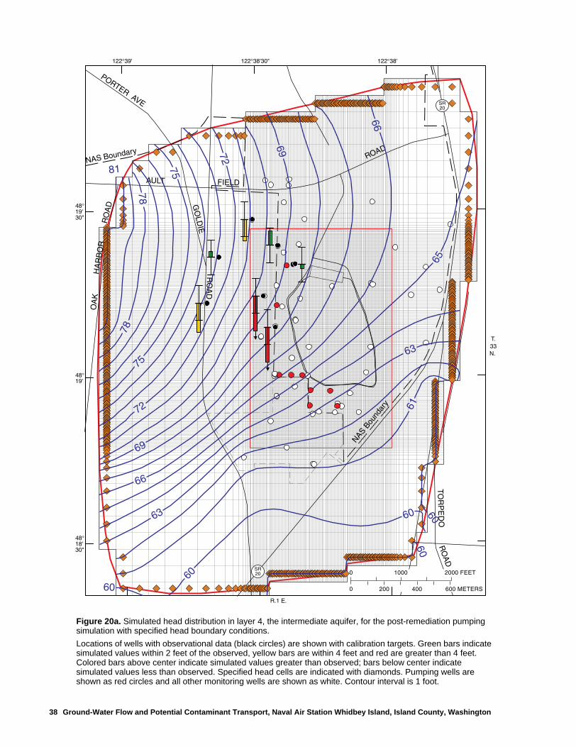
Figure 20a. Map showing simulated head distribution in layer 4, the intermediate aquifer, for the post-remediation pumping simulation with specified head boundary conditions ............................ 38

Figure 20b. Graph showing comparison of simulated and observed heads in wells with screens in the intermediate aquifer for the post-remediation period and a summary of error ................................ 39

Figure 21. Diagram showing comparison of fluxes for model runs using no-flow and specified-head boundary conditions for all cells within the area of primary concern .............................................. 40

Figure 22. Map showing flow paths of particles placed in the vicinity of the contaminant source area indicated by elevated soil gas readings............................................................................................. 42

Contents v

vi Contents

TABLES

Table 1. Precipitation data for Whidbey Island and nearby areas, 1994–98 .................................................. 19Table 2. Hydrologic parameters used in the steady-state model ..................................................................... 27Table 3. Results of sensitivity analysis ........................................................................................................... 30Table 4. Flow rates in extraction wells ........................................................................................................... 31Table 5. Model-derived volumetric ground-water budget for three scenarios ............................................... 43Table 6. Summary of well data ....................................................................................................................... 48

Conversion Factors vii

CONVERSION FACTORS AND VERTICAL DATUM

Temperature in degrees Celsius (°C) may be converted to degrees Fahrenheit (°F) as follows:

°F=1.8 °C+32

Sea level: In this report "sea level" refers to the National Geodetic Vertical Datum of 1929 (NGVD of1929)--a geodetic datum derived from a general adjustment of the first-order level nets of both theUnited States and Canada, formerly called Sea Level Datum of 1929.

Multiply By To obtain

Lengthinch (in) 25.4 millimeterfoot (ft) 0.3048 meter

mile (mi) 1.609 kilometerArea

acre 4,047 square meteracre 0.004047 square kilometer

square mile (mi2) 2.590 square kilometer Volume

gallon (gal) 3.785 literFlow rate

foot per day (ft/d) 0.3048 meter per dayfoot per year (ft/yr) 0.3048 meter per year

cubic foot per day (ft3/d) 0.02832 cubic meter per daygallon per minute (gal/min) 0.06309 liter per second

gallon per day (gal/d) 0.003785 cubic meter per dayinch per year (in/yr) 25.4 millimeter per year

Simulation of Ground-Water Flow and Potential Contaminant Transport at Area 6 Landfill,Naval Air Station Whidbey Island,Island County, Washington

By F. William Simonds

ABSTRACT

A three-dimensional finite-difference steady-state ground-water flow model was developed to simulate hydraulic conditions at the Area 6 Landfill, Naval Air Station Whidbey Island, near Oak Harbor, Washington. Remediation efforts were started in 1995 in an attempt to contain trichloroethene and other contaminants in the ground water. The model was developed as a tool to test the effectiveness of the pump-and-treat remediation efforts as well as alternative remediation strategies. The model utilized stratigraphic data from approximately 76 Navy and 19 private wells to define the geometry of the shallow, intermediate, and deep aquifers and the intervening confining layers.

Initial aquifer parameters and recharge estimates from aquifer tests and published remedial investigation reports were used in the model and then adjusted until simulated water levels closely matched observed water-level data collected prior to the onset of remediation in 1995. The calibrated model was then modified to depict the remedial pump-and-treat system, in which contaminated ground water is extracted, treated, and returned to the ground surface for infiltration. The water levels simulated by the modified model were compared with observed water levels for the 1998 calendar year, during which time the pump-and-treat system was in nearly continuous operation and the ground-water system had equilibrated to steady-state conditions. Although artificial boundaries were used in the model, the choice of model boundary conditions was

determined not to have a significant effect on flow simulation in the area of primary concern surrounding the western contaminant plume and extraction wells. Particle tracking results indicate that the model can effectively simulate the advective transport of contaminants from the source area to the pumping wells and thus be used to test alternative remedial pumping strategies.

INTRODUCTION

The United States Naval Air Station (NAS) at Whidbey Island, Washington, was commissioned in 1942 and served as one of the most important facilities in the Northwest for operation and maintenance of patrol squadrons during World War II. Located on the largest island in the Puget Sound lowland (fig. 1), the base continues to serve as a strategic air base and training facility. From 1942 to about 1992, municipal and industrial wastes generated at the base facilities were disposed of in onsite landfills, open trenches, or by burning. Although considered acceptable at the time, past waste disposal practices have produced potential health and environmental concerns through the release of hazardous contaminants into the soil and ground water.

Within Area 6, a 260-acre tract in the southeastern corner of Ault Field (fig. 2), there are two known waste-disposal areas: a hazardous-waste storage area and a 40-acre landfill. The hazardous-waste storage area is a 4.5-acre tract located to the northwest of the former landfill where an “acid” pit (used for disposal of acids, caustics, and solvents), an oily-sludge pit, waste oil tanks, and a solvent/caustics waste tank were all located.

Abstract 1

Crescent Harbor

City of Oak Harbor

0

0 1

1

2

2

3 MILES

3 KILOMETERS Strait of

Juan de Fuca DuguallaBay

OakHarbor

AULT FIELD

SEAPLANE BASE

Area 6

Area of primaryconcern

Oak HarborLandfill

Naval Air StationWhidbey Island

Seattle

Tacoma

WASHINGTON

Area 6Landfill

S

TATE

H

IGHW

AY

20

Area modeled

NAS Whidbey

Island

PortTownsend

Seattle

Pug

et S

ound

SR20

SR20

Coupeville

Whidb

ey

I s l a n

d

Crescent Harbor

City of Oak Harbor

0

0 1

1

2

2

3 MILES



OakHarbor

AULT FIELD

SEAPLANE BASE

Area 6


Oak HarborLandfill


Seattle

Tacoma

WASHINGTON

Area 6Landfill

S

TATE

H

IGHW

AY

20

Area modeled

NAS Whidbey

Island

PortTownsend

Seattle

Pug

et S

ound

SR20

SR20

Coupeville

Whidb

ey

I s l a n

d

Crescent Harbor

City of Oak Harbor

0

0 1

1

2

2

3 MILES



OakHarbor

AULT FIELD

SEAPLANE BASE

Area 6


Oak HarborLandfill


Seattle

Tacoma

WASHINGTON

Area 6Landfill

S

TATE

H

IGHW

AY

20

Area modeled

NAS Whidbey

Island

PortTownsend

Seattle

Pug

et S

ound

SR20

SR20

Coupeville

Whidb

ey

I s l a n

d

2 G

Figure 1. Location of the Whidbey Island Naval Air Station and Area 6 landfill study area, Island County, Washington.(From URS Consultants, 1993a.)

round-Water Flow and Potential Contaminant Transport, Naval Air Station Whidbey Island, Island County, Washington

The 40-acre landfill at Area 6 was used primarily to dispose of Navy household municipal waste from 1969–92. The landfill accepted solid waste, asbestos, wood, rubble, animal remains, construction debris, and hazardous liquids or sludge. The base of the landfill was not lined. Disposal at the landfill began at the northern end and progressed southward. An estimated maximum of 2.2 million gallons of liquids and sludge containing hazardous wastes was reportedly disposed of in the northern two-thirds of the landfill from 1969–83.

Immediately southwest of Area 6, the City of Oak Harbor operated a 70-acre landfill in a former borrow pit from 1953-82 (fig. 2). Approximately 129 tons of dry-cleaning wastes were reportedly disposed of in the Oak Harbor landfill, along with domestic wastes, demolition materials, and sewage sludge (Ecology and Environment, 1988). A sewage-sludge disposal area was located immediately south of Navy monitoring wells PW-4, 6-S-29, and 6-S-19, and a mixed municipal-waste disposal area is located about 300 feet south of Navy wells PW-5, PW-6, and PW-7. Although the site has not been fully characterized, the quality of ground water beneath the landfill has been monitored regularly at four locations during the 1990’s (R. Knudson, City of Oak Harbor, written communication, 1998).

The Navy started remediation efforts in 1995 to contain trichloroethene (TCE) and other contaminants in the ground water at the Area 6 Landfill by capping the landfill and installing an extraction, treatment and recharge system (referred to as a pump-and-treat system). In 1997, the U.S. Geological Survey began a study in cooperation with the Navy to develop a tool that could test the effectiveness of the pump-and-treat remediation efforts and alternative remediation strategies.

Background

Ground water beneath Area 6 has been sampled multiple times since 1988, confirming that the shallow aquifer is currently contaminated with trichloroethene (TCE), 1,1,1-trichloroethane (TCA), and other volatile organic compounds (VOCs) that are probable degradation products of TCE and TCA. Two somewhat distinct contaminant plumes were identified at the site, one that begins beneath the former hazardous-waste storage area and spreads southward along the western

site boundary, and a second that begins beneath the former landfill and also spreads southward (fig. 2). The western plume is primarily TCA, and TCE and the degradation products cis-1, 2-dichloroethene (cisDCE), 1,1-dichloroethane (DCA), and 1,1-dichloroethene (DCE). The eastern plume is primarily landfill leachate with TCA and the degradation products DCA and vinyl chloride (VC).

In 1989, the Washington Department of Health sampled 13 public wells located within a 1-mile radius of Area 6 and the City of Oak Harbor landfill and found no detectable VOCs. Again in 1991, the Department of Health sampled one public well and six private wells in the vicinity of Area 6 and found no evidence of contamination in any of the wells. Six private water-supply wells located within a 1-mile radius of Area 6 were sampled again in 1994, and no VOCs were detected. As a precautionary measure, however, the Navy began a program offering voluntary water hookups to the public water-supply system for landowners that could potentially be affected, and many wells were subsequently abandoned.

The remedial action selected for treating contaminated ground water at Area 6 included capping the landfill and installing an extraction, treatment, and recharge system (URS Consultants, 1993b). The goals of the remedial action include preventing landfill leachate from reaching ground water, preventing further spread of VOCs, and reducing concentrations of contaminants in the shallow aquifer, with the ultimate goal of meeting State and Federal drinking water standards at specified points of compliance.

The ground-water extraction and treatment system began operation on June 27, 1995; the landfill cap was completed in 1996. From the outset, the pump-and-treat system encountered numerous operational difficulties due to fouling of extraction and treatment equipment and the subsurface drains and reinjection wells by bacteria and iron precipitates (Personal Communication, Sonia Murphy, U.S. Navy, Poulsbo, Washington, 1999; Hart Crowser, 1999a). Most of the recharge-related difficulties were overcome by discharging treated water into an intermittent stream located in a swale just northeast of the landfill and allowing it to infiltrate to the water table; most of the infiltration occurs in the vicinity of monitoring well 6-S-26. Fouling problems in extraction wells and treatment equipment still remain, despite additional recommended maintenance procedures (Hart Crowser, 1999b).

Introduction 3

0

0

1500 FEET

500 METERS

Sw

ale

P-6

N6-38

N6-37

Ault Field Road

State

Hig

hway

20

Gol

die

Roa

d

T.33 N.

R.1 E.

EXPLANATION

Wetland

Area 6 Landfill

Boundary of area of primary concern

Retention pond

Location of hydrogeologic section shown in figure 3

A'AWestern plume - predominantly (TCA)1,1,1-trichloroethane, (TCE)trichloroethene and degradation products

Eastern plume - predominantly (TCA)1,1,1-trichloroethane, (DCA)1,1-dichloroethane, and (VC)vinyl chloride

Monitoring well

Pumping well

Shallow aquifer well

Naval Air Station Boundary

Former 4.5-acrehazardous wastestorage area andother contaminantsources

A'

A

Road

Oak Harbor Landfill

MW-9

MW-6

MW-5

MW-8

MW-10

MW-7MW-14

MW-11

MW-1MW-3B

MW-1

PW-9

PW-8PW-2

PW-4

PW-6

PW-3

PW-1

PW-5 PW-7

PW-4

6-S-276-S-28

6-S-17

6-S-16

6-S-6

6-S-126-S-24

6-S-25

6-S-13

6-S-4

6-S-23

6-S-14

6-S-11 6-S-156-S-9

6-S-2

6-S-7

6-S-26

6-S-106-S-21

6-S-22

6-S-196-S-296-S-3

6-S-25

4 G

Figure 2. Location of Area 6 landfill and surrounding features, including selected wells, hazardous waste storage area, and contaminant plumes.


Purpose and Scope

The purpose of this study was to develop a tool that could be used at some later time to evaluate the effectiveness of the current remediation system in containing the western contaminant plume and to compare alternative remediation strategies. A three-dimensional finite-difference, steady-state ground-water flow model for the Area 6 landfill and vicinity was developed to provide a detailed depiction of the hydrologic system with the flexibility to be modified to simulate a variety of stresses on the system. This report describes the three-dimensional ground-water flow model and how it was developed, calibrated, and tested. The model was developed specifically for the Area 6 landfill site and is focused primarily on the former hazardous-waste storage area, western contaminant plume, and extraction wells. The source area for the eastern plume from the landfill itself is not well known enough to realistically simulate the extent of contamination in that area. The sensitivity of the flow regime, within the area of primary concern, to boundary conditions, hydrologic parameters, and other assumptions also was evaluated. The Navy intends to use the model to test the effects of operating fewer extraction wells, to optimize the location of new monitoring wells for a proposed monitored natural attenuation remedy (Dinicola, 2000), and to conduct more detailed modeling of the contaminant plume. The model differs from previous models constructed for the site in that it incorporates stratigraphic data from more Navy and private wells and is a three-dimensional representation of the hydraulic flow regime.

The model input files used in this study can be obtained on CD-ROM from the USGS District Office in Tacoma, Wash.

Description of the Study Area

NAS Whidbey is located on Whidbey Island in Island County, Washington, on the north end of Puget Sound and the eastern end of the Strait of Juan de Fuca (fig. 1). The island is from 1 to 10 miles wide and almost 40 miles long. The topography of Whidbey Island is characterized by rolling uplands 100-300 feet above sea level, with steep bluffs along the coast. NAS Whidbey is located on the northern part of the island, just north of the City of Oak Harbor (population about 15,000). Forests cover the largest percentage of the island, and urban and agricultural areas cover the

remainder. Land use in the vicinity of Area 6, NAS Whidbey is primarily residential with small commercial areas and open forested or cleared tracts. The former City of Oak Harbor Landfill is immediately southwest of Area 6.

Whidbey Island has a temperate marine climate characterized by warm, dry summers and cool, wet winters. Mean annual temperature is about 50°F; January is the coolest month and August is the warmest. Mean annual precipitation ranges from 18 inches in the northern part of the island to 34 inches in the southern part; that for NAS Whidbey is about 20 inches. Snowfall averages less than 8 inches per year (in/yr), and rainstorms are generally not intense. There are no perennial streams draining the study area, and surface water from extreme storm runoff drains to the north into wetlands near the runways at Ault Field (Dinicola and others, 2000).

Previous Investigations

The Navy was prompted to begin remedial actions at the site by a concern that contaminants could be readily transported in the underlying ground water from the base and into nearby public and private wells on neighboring properties. An Initial Assessment Study (IAS) of all Naval Air Station facilities was conducted in 1984 to identify potential threats to human health or the environment caused by past hazardous-materials handling and disposal practices (Naval Energy and Environmental Support Activity, 1984). The IAS report identified a total of 35 sites as potential sources of contamination that were grouped into 11 areas for further investigation and possible remedial action. Monitoring wells were drilled and a confirmation study was conducted in 1987 to verify and characterize the extent of the contamination (SCS Engineers, 1988). In February 1990, the Ault Field facility was included as a Superfund site on the EPA’s National Priorities List. In response to EPA’s listing and continued concerns about the migration of VOCs in ground water, a Record of Decision was signed in 1993 that committed the Navy to construct a ground-water extraction and treatment system at Area 6 (URS Consultants, 1993a). A Remedial Investigations report was also prepared in 1993 describing the results of extensive characterization of the site and available information on distribution of contamination (URS Consultants, 1993b).

Introduction 5

The ground-water extraction, treatment, and recharge system was installed and began operation in 1995. The system currently extracts, treats, and recharges approximately 275,000 gallons per day.

Four regional ground-water models were developed by the U.S. Geological Survey (USGS) for Island County to evaluate the potential for seawater intrusion into public water-supply wells on Whidbey and Camano Islands (Sapik and others, 1987). These models provided the regional framework for later ground-water models developed specifically for the Area 6 landfill facility.

To aid in design and operation of the pump-and-treat system, a two-dimensional numerical flow model for Area 6 was constructed using FLOWPATH version 4 (IT Corporation, 1993; 1996; 1997). The purpose of the two-dimensional model was to determine the optimal locations for installation of extraction and monitoring wells. Later versions of the model were used to evaluate different remediation strategies by varying pumping rates and locations of treated effluent recharge sites (IT Corporation, 1996, 1997).

When bacteria and iron precipitate buildup began clogging treated effluent reinjection wells, the USGS was asked to evaluate the effect on the regional ground-water system if treated water was not recharged to the aquifer. The USGS model developed for northern Whidbey Island (Sapik and others, 1987) was modified to simulate the effect of pumping ground water from wells at the Naval Air Station, Area 6 landfill facility (E.A. Prych, written communication, 1997). Although the simulation showed only minor regional effects, the need for a more detailed three-dimensional model utilizing refined local stratigraphy and more accurate hydraulic parameters became apparent.

Hydraulic conductivity estimates made during the initial remedial investigation ranged over two orders of magnitude (URS Consultants, 1993b). Multiple well aquifer tests at four of the extraction wells were conducted in June 1998 to obtain more reliable aquifer characteristics (Foster Wheeler Environmental Corporation, 1998b). The results of the 1998 aquifer tests yielded hydraulic conductivity values slightly higher than those used in the two-dimensional ground-water model. The two-dimensional FLOWPATH model was updated later in 1998 to account for the new aquifer-test data and to correct several errors in the previous model (Foster Wheeler Environmental Corporation, 1998a).

Acknowledgments

The author gratefully acknowledges the cooperation and support of Sonia Murphy, Douglas Thelin, and John Gordon of the Naval Facilities Engineering Command, Engineering Field Activity Northwest. Richard Wice of the International Technology Corporation and Tom Goodlin of the Foster Wheeler Environmental Corporation provided geologic information, water-level data and well construction specifications. Henry Bauer, Sue Kahle, and Marijke Van Heeswijk were invaluable resources and provided feedback throughout the study. The report greatly benefited from editorial reviews by James Lyles, Ginger Renslow, and John Clemens and illustration support by Robert Crist.

HYDROGEOLOGY OF THE GROUND- WATER FLOW SYSTEM

Island County lies within the Puget Sound lowland, a topographic and structural depression between the Cascade Range on the east and the Olympic Mountains on the west. Whidbey Island is composed of unconsolidated Pleistocene glacial and interglacial deposits overlying Tertiary and older bedrock (Easterbrook and Anderson, 1968). The unconsolidated deposits range in thickness from a few hundred to 3,000 feet thick and represent deposits from at least three glaciations (Sapik and others, 1987). Surficial deposits consist of unconsolidated sand and gravel with local exposures of more densely compacted glacial till and widely scattered glacial erratic boulders.

Geologic Framework and Hydrologic Units

Ground water in the vicinity of NAS Whidbey generally occurs within a series of aquifers composed of permeable sand-and-gravel layers deposited by glacial melt water, separated by finer grained glacial silt-and-clay or interglacial fluvial and lacustrine deposits (URS Consultants, 1993b). These subsurface materials have been locally characterized into six hydrogeologic units (URS Consultants, 1993b; Sapik and others, 1987). These units are the Vashon till, Vashon advance outwash, and four subunits of the Whidbey Formation.

6 Ground-Water Flow and Potential Contaminant Transport, Naval Air Station Whidbey Island, County, Washington

Beneath Area 6, the upper 200 feet of sediments contain three principal water-bearing units, referred to as the shallow, intermediate, and deep, or sea level, aquifers (fig. 3).

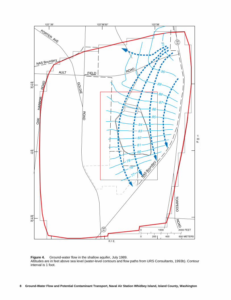
The shallow aquifer is contained within the Vashon advance outwash sediments. It is a major water-bearing zone in the region and extends throughout all of Area 6. The shallow aquifer contains the largest contaminant concentrations and is the primary focus of this and previous investigations. Although some water can be found perched above the glacial till in small portions of Area 6, the shallow aquifer is generally unconfined, with water levels ranging from about 20 to 145 feet below the ground surface. Ground-water flow directions are toward the southwest in the northern part of the area and toward the southeast in the southern part, forming a generally

accurate path from north to south (fig. 4). North of the study area, a poorly defined flow divide separates a component of flow to the northwest towards Ault Field. Stratigraphy and thickness data are available from 44 Navy and various private wells that fully penetrate the Vashon advance outwash (see table 6 at end of report). The Vashon advance outwash is a medium to coarse sandy gravel or gravely sand that becomes finer grained with depth. Including Vashon till where present, the thickness of Vashon advance outwash ranges from 21 feet to 176 feet thick within the study area (fig. 5). However, the saturated portion of the deposit ranges from 13 feet to 61 feet thick and averages 30 feet thick. The horizontal hydraulic conductivity is estimated to be 87 feet per day (ft/d) for the upper portion of the unit, and 70 ft/d for the lower, finer grained portion of the unit.

Figure 3. Generalized hydrogeologic section showing distribution of aquifer and confining units and the numbered layers used in the ground-water model.(Modified from Dinicola, 2000.) See figure 2 for trace of section.

Intermediate aquifer

Deep or sea-level aquifer

Shallow aquifer

Upper confining unit

Lower confining unitClay, sand, silt

Medium to coarse sandygravely or gravely sand

Clay, sand, siltSand,silt with some clay

Medium to coarse sandwith some gravel

Till

Silty sandSubunit 13

4

5

6

2

1

Subunit 2

Subunit 3

Subunit 4

Vashon till

Modellayers

North250

200

150

100

50

50

100A

LTIT

UD

E, I

N F

EE

T

SEALEVEL

6-S-26

6-S-10

6-S-22

6-S-156-S-236-S-14

6-S-256-S-13 B

EN

D IN

SE

CT

ION

BE

ND

INS

EC

TIO

N

BE

ND

INS

EC

TIO

N

South

~5x Vertical exaggeration

Vashonadvanceoutwash

WhidbeyFormation

0 500 1000 FEET

0 100 200 300 METERS

Intermediate aquifer

Deep or sea-level aquifer

Shallow aquifer

Upper confining unit

Lower confining unitClay, sand, silt

Medium to coarse sandygravely or gravely sand

Clay, sand, siltSand,silt with some clay

Medium to coarse sandwith some gravel

Till

Silty sandSubunit 13

4

5

6

2

1

Subunit 2

Subunit 3

Subunit 4

Vashon till

Modellayers

North250

200

150

100

50

50

100A

LTIT

UD

E, I

N F

EE

T

SEALEVEL

6-S-26

6-S-10

6-S-22

6-S-156-S-236-S-14

6-S-256-S-13 B

EN

D IN

SE

CT

ION

BE

ND

INS

EC

TIO

N

BE

ND

INS

EC

TIO

N

South

~5x Vertical exaggeration

Vashonadvanceoutwash

WhidbeyFormation

0 500 1000 FEET

0 100 200 300 METERS

Hydrogeology of the Ground- Water Flow System 7

SR20

SR20

PORTER AVE

GO

LDIE

RO

AD

FIELDAULT ROAD

RO

AD

TOR

PE

DO

NAS Boundary

NAS Bou

ndar

y

RO

AD

HA

RB

OR

OA

K

0

0

1000 2000 FEET

200 400 600 METERS

48° 19'30"

48° 18'30"

48° 19'

122°38'30" 122°38'122° 39'

T.33N.

87

86

85

84

83

82

81

80

79

78

77

90

91

89

88

SR20

SR20

PORTER AVE

GO

LDIE

RO

AD

FIELDAULT ROAD

RO

AD

TOR

PE

DO

NAS Boundary

NAS Bou

ndar

y

RO

AD

HA

RB

OR

OA

K

0

0

1000 2000 FEET

200 400 600 METERS

48° 19'30"

48° 18'30"

48° 19'

122°38'30" 122°38'122° 39'

T.33N.

R.1 E.

87

86

85

84

83

82

81

80

79

78

77

9091

89

88

8 G

Figure 4. Ground-water flow in the shallow aquifer, July 1989. Altitudes are in feet above sea level (water-level contours and flow paths from URS Consultants, 1993b). Contour interval is 1 foot.


150

150

140

130

120

90

9010

011

0

120

90

100

110

6070

70

80

60

70

30

30

40

5060

30

40

50

80

140150160

150

170

130

120

11010090

120

80

50

50

40

60

6040

7011

0

100

90

120

8080

130

140

SR20

SR20

PORTER AVE

GO

LDIE

RO

AD

FIELDAULT

ROAD

RO

AD

TOR

PE

DO

NAS Boundary

NAS Bou

ndar

y

RO

AD

HA

RB

OR

OA

K

0

0

1000 2000 FEET

200 400 600 METERS

T.33N.

R.1 E.

6-S-10

6-S-7

P-2

P-3P-4

P-1

Dickson

6-S-20

A381

6-S-22

PW-1

PW-6

MW-8

MW-7

PW-7

Rodewald

MW-10

6-S-21

6-S-17

6-S-296-S-19

MW-1

MW-9

6-S-13

6-S-276-S-28

6-S-12

6-S-18

MW-11

MW-15

PW-5

PW-4

6-S-11

6-S-15

MW-12

PW-3

MW-3b

MW-6

MW-13

6-S-16

6-S-2

6-S-14

MW-14

N6-37N6-38

6-S-8

6-S-5

PW-2 PW-8

PW-9

6-S-1

6-S-3

6-S-24

6-S-9

6-S-23

MW-2

MW-4

6-S-4

P-8P-7

P-6

6-S-25

P-5

6-S-6

MW-5

MW-3a

DOE

6-D-4

OakHarbor

6-D-1

6-D-2

6-D-3

6-I-1

Hilberdink

6-I-8

6-I-5

6-I-6

6-I-7

M&Eenterprizes

6-S-26

6-I-2

6-I-4

6-I-3

Figure 5. Thickness of Vashon advance outwash deposits in Area 6, including Vashon till where present.Contour interval is 10 feet. Wells that provide stratigraphic information for the shallow aquifer are shown in green, and the deep aquifer are shown in red. (Stratigraphic data from URS Consultants,1993b, and summarized in Appendix A.)


The uppermost subunit 1 in the Whidbey Formation is a confining unit consisting of dark green clay and fine sands and silts with minor peat and wood material that immediately underlies the shallow aquifer. The confining unit is generally about 10 feet thick, but can vary from 1 foot to 40 feet thick within the study area (fig. 6). Because of the fine-grained nature of the material, the hydraulic conductivity for this unit is estimated to be 0.0002 foot per day.

The intermediate aquifer is defined as subunit 2 of the Whidbey Formation. Although not a major water-bearing zone in the region, it extends throughout northern Whidbey Island. Only very low concentrations of contaminants have been detected within this aquifer beneath Area 6. The intermediate aquifer is generally confined, and water levels are generally 5 to 20 feet lower than those in the shallow aquifer. Ground-water flow directions in the intermediate aquifer are poorly defined, but are generally from the northwest to the southeast (fig. 7). Limited stratigraphic and thickness data are available from 13 Navy and two private wells that fully penetrate subunit 2 of the Whidbey Formation (see table 6). The subunit consists of sand and silts or fine sand and may contain thin, discontinuous, dark-gray silty clay layers. Thickness of the unit varies from 4 feet to 69 feet thick within the study area (fig. 8). The horizontal hydraulic conductivity for this unit is estimated to be 10 ft/d.

Subunit 3 of the Whidbey Formation is a confining unit consisting of dark-colored clay, sand, and silts with gravel or silty clay layers and woody material, and immediately underlies the intermediate

aquifer. The confining unit varies from 5 feet to 54 feet thick within the study area (fig. 9). Because of the fine-grained nature of the material, the hydraulic conductivity for this unit is estimated to be 0.0002 ft/d.

The deep, or sea level, aquifer is defined by subunit 4 of the Whidbey Formation. This unit is a continuous water-bearing zone in the region. No contaminants have been detected in this aquifer beneath Area 6, with the exception of those resulting from a now abandoned, poorly constructed monitoring well. The aquifer is confined, with water levels ranging from 11 to 17 feet above sea level. Ground-water flow direction in the deep aquifer is not well known but is generally towards the southwest. Very limited stratigraphic and thickness data are available from 4 Navy wells and 1 private well that intercepts the deep aquifer (see table 6). Only one deep drill hole, just northwest of the study area, penetrates the entire section of glacial deposits and is finished in bedrock at a depth of 531 feet below land surface. Subunit 4 of the Whidbey Formation consists of medium to coarse sand with gravel. The thickness of subunit 4 is estimated to be about 240 feet, based on the one deep drill hole. However, the aquifer thickness may be as much as 450 feet because the underlying Double Bluff Formation consists of similar sand and gravel glacial outwash material and the aquifer could continue into it.


SR20

SR20

PORTER AVE

GO

LDIE

RO

AD

FIELDAULT

ROAD

RO

AD

TOR

PE

DO

NAS Boundary

NAS Bou

ndar

y

RO

AD

HA

RB

OR

OA

K

0

0

1000 2000 FEET

200 400 600 METERS

T.33N.

R.1 E.

303540 25

15

20

15

30

15

152025

155

1020 10 5

25

1520

10

5

10 10

1010

10

6-S-10

6-S-7

P-2

P-3P-4

P-1

Dickson

6-S-20

A381

6-S-22

PW-1

PW-6

MW-8

MW-7

PW-7

Rodewald

MW-10

6-S-21

6-S-17

6-S-296-S-19

MW-1

MW-9

6-S-13

6-S-276-S-28

6-S-12

6-S-18

MW-11

MW-15

PW-5

PW-4

6-S-11 6-S-15

MW-12

PW-3

MW-3b

MW-6

MW-13

6-S-16

6-S-2

6-S-14

MW-14

N6-37

N6-38

6-S-8

6-S-5

PW-2PW-8

PW-9

6-S-1

6-S-3

6-S-24

6-S-9

6-S-23

MW-2

MW-4

6-S-4

P-8

P-7

P-6

6-S-25

P-5

6-S-6

MW-5

MW-3a

DOE

6-D-4

OakHarbor

6-D-1

6-D-2

6-D-3

6-I-1

Hilberdink

6-I-8

6-I-5

6-I-6

6-I-7

M&Eenterprizes

6-S-26

6-I-2

6-I-4

6-I-3

Figure 6. Thickness of subunit 1 of the Whidbey Formation that defines the upper confining unit, or layer 3 of the model.Contour interval is 5 feet. Wells that provide stratigraphic information for the upper confining unit are shown in black, green, and red. (Stratigraphic data from URS Consultants,1993b, and summarized in Appendix A.),


SR20

SR20

PORTER AVE

GO

LDIE

RO

AD

FIELDAULT

ROAD

RO

AD

TOR

PE

DO

NAS Boundary

NAS Bou

ndar

y

RO

AD

HA

RB

OR

OA

K

0

0

1000 2000 FEET

200 400 600 METERS

N

R.1 E.

75

70

65

60

70

65

60

12 G

Figure 7. Ground-water flow in the intermediate aquifer, November 1991.Altitudes are in feet above sea level (water-level contours and flow paths from URS Consultants, 1993b). Contour interval is 5 feet.


SR20

SR20

PORTER AVE

GO

LDIE

RO

AD

FIELDAULT

ROAD

RO

AD

TOR

PE

DO

NAS Boundary

NAS Bou

ndar

y

RO

AD

HA

RB

OR

OA

K

0

0

1000 2000 FEET

200 400 600 METERS

T33N

R.1 E.

6065

60

45

35

40

4550

55

45

403530

30

30

30

30

30

30

30

15

25

25

20

20

1510

5

4540

35

5055

2525

10

306-S-10

6-S-7

P-2

P-3P-4

P-1

Dickson

6-S-20

A381

6-S-22

PW-1

PW-6

MW-8

MW-7

PW-7

Rodewald

MW-10

6-S-21

6-S-17

6-S-29

6-S-19

MW-1

MW-9

6-S-13

6-S-276-S-28

6-S-12

6-S-18

MW-11

MW-15

PW-5

PW-4

6-S-11 6-S-15

MW-12

PW-3

MW-3b

MW-6

MW-13

6-S-16

6-S-2

6-S-14

MW-14

N6-37N6-38

6-S-8

6-S-5

PW-2 PW-8

PW-9

6-S-1

6-S-3

6-S-24

6-S-9

6-S-23

MW-2

MW-4

6-S-4

P-8P-7

P-6

6-S-25

P-5

6-S-6

MW-5

MW-3a

DOE

6-D-4

OakHarbor

6-D-1

6-D-2

6-D-3

6-I-1

Hilberdink

6-I-8

6-I-5

6-I-6

6-I-7

M&Eenterprizes

6-S-26

6-I-2

6-I-4

6-I-3

Figure 8. Thickness of subunit 2 of the Whidbey Formation that defines the intermediate aquifer, or layer 4 of the model.Contour interval is 5 feet. Wells that provide stratigraphic information for the intermediate aquifer are shown in green and red. (Stratigraphic data from URS Consultants,1993b, and summarized in Appendix A.)


SR20

SR20

PORTER AVE

GO

LDIE

RO

AD

FIELDAULT

ROAD

RO

AD

TOR

PE

DO

NAS Boundary

NAS Bou

ndar

y

RO

AD

HA

RB

OR

OA

K

0

0

1000 2000 FEET

200 400 600 METERS

T.33N.

R.1 E.

45

4540

35

50

45

30

25

20

35

40

40

30

2520

15 105

15

1510 20 25 30 35 40

10

10

2025

6-S-10

6-S-7

P-2

P-3P-4

P-1

Dickson

6-S-20

A381

6-S-22

PW-1

PW-6 MW-8

MW-7

PW-7

Rodewald

MW-10

6-S-21

6-S-17

6-S-296-S-19

MW-1

MW-9

6-S-13

6-S-27

6-S-28

6-S-12

6-S-18

MW-11

MW-15

PW-5

PW-4

6-S-11 6-S-15

MW-12

PW-3

MW-3b

MW-6

MW-13

6-S-16

6-S-2

6-S-14

MW-14

N6-37N6-38

6-S-8

6-S-5

PW-2 PW-8

PW-9

6-S-1

6-S-3

6-S-24

6-S-9

6-S-23

MW-2

MW-4

6-S-4

P-8P-7

P-6

6-S-25

P-5

6-S-6

MW-5

MW-3a

DOE

6-D-4

OakHarbor

6-D-1

6-D-2

6-D-3

6-I-1

Hilberdink

6-I-8

6-I-5

6-I-6

6-I-7

M&Eenterprizes

6-S-26

6-I-2

6-I-4

6-I-3

14 G

Figure 9. Thickness of subunit 3 of the Whidbey Formation that defines the lower confining unit, or layer 5 of the model.Contour interval is 5 feet. Wells that provide stratigraphic information for the lower confining unit are shown in red. (Stratigraphic data from URS Consultants, 1993b, and summarized in Appendix A.)


Hydraulic Properties of Aquifers and Confining Units

The hydraulic conductivity of the aquifers and confining units depends on the density and viscosity of the fluid and the grain size, shape, sorting, and packing of the matrix material (Freeze and Cherry, 1979). In this study, no seawater is involved and density/viscosity effects of the contaminants are assumed to be negligible, so the fluid (water) of the regional flow system is assumed to have a constant density and viscosity. Earlier published hydraulic conductivity data for the shallow, intermediate, and deep aquifers beneath the Area 6 landfill are derived from single-well pumping tests, slug tests and associated grain-size analyses, and laboratory tests (URS Consultants, 1993b). The resulting hydraulic conductivities varied widely, so in 1998 Navy contractors conducted additional multiple-well pumping tests at extraction wells PW-1, PW-3, PW-5, and PW- 9 to better define the values. Each test used one extraction well and 6 to 10 nearby observation wells (Foster Wheeler Environmental Corporation, 1998b). The multiple-well pumping tests yielded horizontal hydraulic conductivity values for the shallow aquifer that ranged from 47 to 126 ft/day (Foster Wheeler Corporation, 1998b). The average hydraulic conductivity for all the wells in the test was 87 ft/day, a value slightly higher than the values (40 to 80 ft/day) used in the previous modeling study (IT Corporation, 1997). The hydraulic conductivity data from the multiple-well pumping tests were considered more reliable and were used as initial estimates in this study.

Horizontal hydraulic conductivities are generally greater than vertical hydraulic conductivities because of the horizontal stratification of coarse and fine matrix materials in the glacial sediments. This vertical anisotropy in hydraulic conductivity occurs in both aquifers and confining units. However, confining units have such low hydraulic conductivities that the horizontal component of flow is considered to be negligible. Thus, a horizontal-to-vertical hydraulic conductivity ratio of 1:1 was assumed for the confining units. For aquifer materials, more reliable hydraulic conductivity data are available. A Neuman analysis conducted on one of the multiple-well pump tests (PW- 3) allowed for direct computation of vertical hydraulic conductivity in the shallow aquifer (Foster Wheeler Corporation, 1998b; Neuman, 1975). Test results indicated that ratios of horizontal to vertical

hydraulic conductivities for the aquifers were on the order of 4:1 to 8:1, or about 5:1 on average (Foster Wheeler Environmental Corporation, 1998b).

The ratio of horizontal to vertical hydraulic conductivity is important in determining the leakance between aquifer and confining layers. Leakance is a function of the layer thickness and the hydraulic conductivity of each layer bounding an interface between layers. Leakance is generally calculated by the equation:

(1)

where

Recharge

Virtually all of the naturally occurring ground-water recharge on Whidbey Island occurs by direct vertical infiltration of precipitation. Very few intermittent streams occur on the island and these flow only during heavy rainfall events. Based on 10 to 40 years of precipitation records, Whidbey Island receives an average annual precipitation of 18 to 34 in/yr; approximately 20 in/yr falls at the study area (Sapik and others, 1987). The amount of that precipitation that recharges the aquifer can be estimated on the basis of the type of land use and associated root-zone depths, as well as on geological considerations such as the presence of glacial till at the surface. Previous recharge estimates by Sapik and others (1987) range from 4 to 8 in/yr for forested land, 6 to 10 in/yr for agricultural land, and 8 to 12 in/yr for barren rangeland. Previous recharge estimates by IT Corporation (1997), based on soil types, ranged from 3.5 to 9.0 in/yr.

Zu is thickness of the upper layer;

Ku is conductivity of the upper layer;

Z1 is thickness of the lower layer; and

K1 is vertical hydraulic conductivity of the lower layer.

Leakage 1Zu

2 Ku×---------------

Z12 K1×---------------+

--------------------------------------=


In this study, the presence of glacial till is assumed to play an important role in governing the amount of precipitation recharging the aquifer system. In areas where highly compacted till with fine particle size mantle the land surface, recharge to the aquifer is limited because of the decreased infiltration capacity of the till (Bauer and Mastin, 1996). Thus, in this study, till-mantled areas are assumed to have a lower recharge value (7.0 in./yr) than areas where till is not present (10.0 in./yr) (fig. 10). The wetland area to the north of the Area 6 landfill is assumed to be an area of high recharge due to the fact that little or no surface flow leaves the wetland. Other wetland areas within the study area represent localized areas of perched water; they are wet only during heavy rain events and do not appear to influence ground-water flow directions in the shallow aquifer.

Remediation activities have changed the distribution of recharge across Area 6. The landfill was capped with an impermeable barrier in 1996, beneath which recharge was essentially eliminated. All precipitation falling on the landfill cap was redirected toward a retention pond (see fig. 10) on the north side of the landfill where it could infiltrate. On June 27, 1995, the treatment plant was started and ground water, extracted through pumping wells, was piped to an air-stripping tower where VOCs could be volatilized and removed. Treated ground water was returned to the shallow aquifer, initially through injection wells, but bacteria and iron precipitates caused clogging problems in the injection wells forcing treated water to be directed to the retention pond. Eventually treated ground water was directed to the intermittent stream north and east of the landfill, where it could infiltrate naturally to the shallow aquifer. All of the treated water usually infiltrates before reaching the wetlands.

STEADY-STATE SIMULATION OF THE GROUND-WATER FLOW SYSTEM

A three-dimensional, steady-state ground-water flow model of the Area 6 landfill was developed as a tool to test the effectiveness of the present pump-and-treat system and to investigate alternative remediation strategies. Specifically, the numerical model is designed to evaluate whether water traveling down gradient from a known former hazardous-waste storage

area is being captured by the existing pumping wells. Other important uses of the model include evaluating the effectiveness of different remediation strategies, such as the effects of operating fewer extraction wells, and helping to optimize the location of new monitoring wells for a proposed monitored natural attenuation remedy (Dinicola, 2000).

Modeling Approach

The ground-water flow system was simulated using Groundwater Modeling System (GMS version 2.1), a commercially available graphical user interface that supports MODFLOW versions 1638 and 1323 (McDonald and Harbaugh, 1988), MODPATH version 3.0 (Pollock, 1994), and other analysis codes. The area modeled in this study extends outside of the Naval Air Station Area 6 boundary but is centered on the western contaminant plume on the west side of the Area 6 landfill (fig. 2). The finite-difference grid used in the model (fig. 11) was designed to provide highest resolution for the area of primary concern, which includes the former hazardous waste storage area, western contaminant plume, extraction wells, and area 6 landfill. Care was taken to locate model boundaries in such a way as to minimize the influence of boundary conditions on the area of primary concern, and to limit the grid size for computational efficiency. Artificial model boundaries had to be used because natural hydrologic boundaries were too far away to be included in this highly localized modeling study. The limitations of the artificial boundaries were tested by specifying different boundary conditions and determining the effect on the area of primary concern.

Two time periods were selected for simulation, a calibration period that represented steady-state conditions prior to the onset of remediation activities, and a post-remediation period that represented steady-state conditions after water levels had stabilized in response to implementation of the pump-and-treat system. No significant commercial or residential pumping stresses are known to exist in the immediate vicinity of Area 6 during either time period; most domestic wells near the base boundary have been abandoned and both NAS Whidbey and the City of Oak Harbor use surface water as their primary water supply.


200

210

120

120

160

140

180

180

160

140

120

100

100

100

110

100

100

100

140

160

180

120

120

40

60

80

80

200

NAS Boundary

Landfill

Cap

Intermittent

Stream

Retention

Pond

Model

Boundary

Wet

Lands

122 38'30"

T.

33

N.

R.1 E.Base map modified from U.S. Geological Survey

Oak Harbor, 1:24,000, 1973

SR

20

SR

20

PO

RTER

GO

LD

IE

RO

AD

FIELDAULT

RO

AD

RO

AD

TO

RP

ED

O

NAS Boundary

RO

AD

HA

RB

OR

OA

K

High recharge (10.0 inches per year)

Low recharge (7.0 inches per year)

Altitude above sea level,

contour interval 20 feet

0

0

1000 2000 FEET

200 400 600 METERS

EXPLANATION

60

NATIONAL GEODETIC VERTICAL DATUM OF 1929

Figure 10. Distribution of recharge values used in the ground-water model.Areas where till is present were assigned the low recharge value and areas where it is absent, the high recharge value.

Steady-State Simulation of the Ground-Water Flow System 17

SR20

SR20

Landfill cap

Intermittent stream

Retention pond

Model boundary

NAS Boundary

NAS Bou

ndar

y

PORTER AVE

GO

LDIE

RO

AD

FIELDAULT

ROAD

RO

AD

TOR

PE

DO

0

0

1000 2000 FEET

200 400 600 METERS

T.33N.

R.1 E.

18 G

Figure 11. Finite-difference grid for the numerical three-dimensional model of ground-water flow at the Area 6 landfill.The red rectangle represents the area of primary concern, with a dense grid of 25-by-25-foot cells.


Water levels in approximately 52 wells were measured three times prior to the onset of remedial activities (IT Corporation, 1995). These water levels, measured on 5/19/94, 1/31/95- 2/1/95, and 6/19/95–6/20/95, were the only data available to constrain the pre-remediation steady-state condition. Although the pre-remediation water levels showed a slight decrease of about 1 foot, the change was likely related to below-normal precipitation (table 1) and recharge in 1994 (fig. 12). For each well, measured water levels were averaged to obtain a representative water level indicative of the pre- remediation, steady-state condition.

The 52 wells measured during the pre-remediation period also were measured on a monthly basis during the post-remediation period along with additional new monitoring wells, a selection of which are shown on figure 12. In order to avoid changes in ground-water storage due to pumping and climatic affects, only water level data from 1998 were used to constrain the simulation of the post-remediation period. These monthly data were averaged to obtain a representative water level indicative of the post-remediation steady-state condition. The unsteady-state transient response to the pump-and-treat system is evident in figure 12 between June 1995 and about December 1997 where water levels were equilibrating to a new steady-state condition. In addition to the new

pumping stress on the system, available precipitation records (table 1) show a slight increase from 1994 to 1998 for the nearby climatological stations at Coupeville and Port Townsend, as well as for the Olympic Mountains and San Juan Islands to the northeast as a whole (table 1; NOAA, 1994, 1995, 1996, 1997, 1998). Thus, the transient ground-water-level response seen from June 1995 to about December 1997 is due to the superimposed effects of the pump-and-treat system and increased precipitation. The water levels in well 6-S-2 (an upgradient well not substantially affected by remediation activities) indicate an increase in ground-water storage from late 1995 through mid 1997, followed by a period of less change. It is noteworthy that after the increase in storage, the water level in 6-S-2 did not recede to the pre-remediation level; this observation is further discussed in the section entitled “Simulation of post-remediation conditions.

The model was calibrated using initial hydraulic parameters derived from published reports. During calibration, the initial hydraulic parameters were adjusted iteratively by trial and error until simulated water levels most closely matched the averaged pre-remediation water levels. As part of the calibration processes a sensitivity analysis was performed to determine which parameters had the greatest affect on the model outcome.

Table 1. Precipitation data for Whidbey Island and nearby areas, 1994–98

Precipitation(inches per year)1

Year Coupeville Port TownsendNE Olympics andSan Juan Division

1998 21.86 (0.84) 23.00 (1.98) 109.82 (12.75)

1997 26.39 (5.37) 21.77 (0.75) 125.40 (28.33)

1996 .no data 21.39 (0.44) 109.04 (11.97)

1995 .no data 23.7 (2.68) 110.87 (13.80)

1994 .no data 13.93 (-7.09) 104.31 (7.24)

1Departure from normal for period of record shown in parentheses; data from National Oceanic and Atmospheric Administration, 1994–98.


20G

rou

nd

-Water F

low

and

Po

tential C

on

tamin

ant T

ransp

ort, N

aval Air S

tation

, Wh

idb

ey Island

, Island

Co

un

ty, Wash

ing

ton

OC

T

DE

C

FE

B

AP

RIL

JUN

E

AU

G

OC

T

DE

C

1998

-S-21

-S-22

-S-23

6-S-25

6-S-27

JUN

E

AU

G

OC

T

DE

C

FE

B

AP

RIL

JUN

E

AU

G

OC

T

DE

C

FE

B

AP

RIL

DATE

19951994 1996

AP

RIL

JUN

E

AU

G

OC

T

DE

C

FE

B

AP

RIL

70

75

80

85

90

95

ALT

ITU

DE

, IN

FE

ET

AB

OV

E S

EA

LE

VE

L

PRE-REMEDIATION REMEDIATION

Selected wells

6-S-2

6-S-3

6-S-4

6-S-6

6-S-7

6-S-8

6-S-10

6-S-11

6-S-12

6-S-15

6-S-19

6-S-20

Non-pumpinginterval

EXPLANATION

Figure 12. Water levels for selected wells screened in the shallow aquifer for the period April 1994 to DecembeGray bars at the base of the graph indicate periods when the pump-and-treat system was not in operation.

JUN

E

AU

G

1997

6

6

6

r 1998.

The calibrated model was then modified to simulate the existing remedial extraction and treatment system by adding nine extraction wells that withdraw water at average rates of flow published in quarterly reports (1995, 1996, 1997, 1998, and 1999). In the model, treated water was returned to the system by adding the extracted volume to recharge cells located along the intermittent stream.

To test the effects of assumed boundary conditions on simulated flow within the area of primary concern, scenarios were run using two different types of boundary conditions. In both scenarios, water-level distributions, fluxes through the area of primary concern, and particle flow paths in the shallow aquifer were compared.

Description of Model

The modeled area is overlain by a rectangular grid with cells that ranged in size from 25 ft to 300 ft on a side (fig. 11). The smallest cells (25 ft by 25 ft) were centered on the area of primary concern, which includes contaminant source areas, extraction wells, and the Area 6 landfill. In the horizontal dimensions, the grid was made up of 189 rows and 130 columns and covered a total area of about 2.5 square miles. The grid was oriented in the north-south direction, roughly parallel to the primary ground-water flow direction. Aquifer materials are assumed to be homogeneous and isotropic and thus, there is no preferred alignment of the transmissivity tensor.

In the vertical dimension, the modeled area was conceptualized as a ground-water flow system with six layers (see fig. 3) based on subsurface geology from lithologic logs from approximately 76 Navy wells and 19 private wells (URS Team, 1998). The unsaturated zone, consisting of surficial gravels, Vashon till, and the upper part of the Vashon advance outwash, was included as part of layer 1 in the model; however, ground-water flow calculations were performed only on the saturated portions of the model. Layer 2 consists of generally finer grained sediments in the lower portion of the Vashon advance outwash. Because the contact between layers 1 and 2 is not well defined on the available lithologic logs, layer 2 was conceptualized as a 10-foot-thick layer with a lower hydraulic conductivity than layer 1. Together, layer 1 and layer 2 comprise the unconfined, shallow aquifer. Layer 3 is a confining layer defined as subunit 1 of the

Whidbey Formation. Horizontal flow through layer 3 was assumed to be insignificant due to the low hydraulic conductivity and presumably small horizontal gradients of hydraulic head. Layer 4 represents the intermediate aquifer and is equivalent to subunit 2 of the Whidbey Formation. Layer 5 is the lower confining unit and is equivalent to subunit 3 of the Whidbey Formation. Horizontal flow through layer 5 was also assumed to be insignificant due to the low hydraulic conductivity and presumably small horizontal gradients of hydraulic head. Layer 6 is the bottom or deepest layer in the model and represents the deep aquifer, or subunit 4 of the Whidbey Formation. Because the depth to bedrock, type of material, and actual thickness of the deep aquifer are unknown, the deep aquifer was assigned an estimated thickness of 250 feet based on one well in the area that penetrates to bedrock

Boundary Conditions

Conditions along the perimeter of the model are important, as they may affect the results of the simulation. Ideally, the location of model boundaries should correspond to actual hydrologic boundaries. However, when hydrologic boundaries cannot be represented realistically in the model, it is important that prescribed boundaries be located far enough away that they do not have an effect on the simulated conditions in the area of primary concern. Of the various types of boundaries typically used in ground-water flow models (Franke and others, 1987), the following types were applicable for use in this study. One type is the streamline or stream-surface (no-flow) boundary, used where the flow is parallel to a boundary and no component of flow crosses the boundary. Here a specified flux of zero was assigned at the boundary. Another type is a specified-head boundary, where head is specified and the flow into or out of the model is allowed to adjust accordingly. The bottom of the model was specified as a constant-head boundary, used to allow flow out the bottom of the model while maintaining the same head value at all points. The top of the model was specified a free-surface boundary, represented by the water table, and allowed to rise and fall as needed in response to recharge and flow through the model.


In this study, care was taken to locate lateral model boundaries perpendicular to previously published ground-water-level contours in the shallow aquifer (layers 1 and 2) so that a no-flow boundary would be a reasonable assumption on the east and west sides of the model (fig. 13). The northern boundary of the model was chosen to coincide with a postulated hydrologic flow divide so that a no-flow assumption would also be reasonable for layers 1 and 2 (see fig. 4). The southern boundary was aligned parallel to ground-water-level contours so that heads could be specified on the basis of projections of observed water-level data. The topography of the study area and conceptual ground-water flow suggests that a wetland area just southeast of the model boundary, and east of Oak Harbor, could be a discharge area for the shallow aquifer. In order to represent this concept, head values near land surface were specified along the southeast corner of the model for layers 1 and 2 to simulate discharge to the wetland.

Limited observed water-level data for the intermediate aquifer (layer 4) indicates that ground-water flow is generally toward the southeast corner of the study area. To simulate flow in the intermediate aquifer, a combination of specified-head and no-flow boundaries were specified along the perimeter of layer 4 (fig. 14). The head values were specified along the western and a portion of the eastern boundaries in such a way as to create flow directions in the corresponding model layer 4 that approximate the observed data.

The lower boundary of the model was defined as the bottom of the deep aquifer (layer 6). Although very few observational data are available for the deep aquifer, data from 1991 and 1992 show a ground-water flow direction to the southwest at a gradient of 0.00015 to 0.006 foot per foot (URS, 1993b). For the purposes of this modeling study the observed gradient was assumed to be insignificant, thus, all cells in layer 6 were assigned a uniform constant head set at 14 feet, equivalent to the average water level observed in wells that penetrate the deep aquifer. All confining units (layers 3 and 5) were assigned no-flow lateral boundaries because any significant flow in these units is assumed to be vertical.

Calibration of Model to Pre-Remediation Conditions

The model was calibrated to the conditions existing before installation of the landfill cap and operation of remedial extraction wells in June 1995. The ground-water system was assumed to be at steady state, based on the absence of any pronounced trends in water levels for the period May 1994 through June 1995 (see fig. 12). The model was calibrated by running MODFLOW simulations and comparing the simulated head values with observed pre-remediation water-level data. Values for recharge, hydraulic conductivity, and specified head cells at model boundaries were systematically adjusted until simulated heads most closely matched pre-remediation water levels and flow directions. Special care was taken to keep values for hydraulic conductivity, recharge, and specified heads within reported limits and not introduce values unsupported by the available data.

Initial values for hydraulic conductivity were established using values from the previous modeling study by IT Corporation (1997) and the results of recent aquifer tests (Foster Wheeler Environmental Corp., 1998b). Hydraulic conductivities for the shallow aquifer were initially applied along northeast to southwest trending zones of 90 ft/d, 85 ft/d, and 75 ft/d. A horizontal to vertical conductivity ratio of 10 to 1 was used initially in the calculation of leakance. Recharge values initially were set in zones of high (10 in/yr), medium (8 in/yr), and low (7in/yr) recharge, similar to the previous modeling study (IT Corporation, 1997). The observed pre-remediation water levels are from published measurements made on May 19, 1994, January 31 to February 1, 1995, and June 19 to 20, 1995 (IT Corporation, 1995). This data set includes 39 wells with screens in the shallow aquifer and 7 wells screened in the intermediate aquifer. Water-level measurements for each well were averaged to obtain a time-averaged representation of the pre-remediation water level.


SR20

SR20

PORTER AVE

GO

LDIE

RO

AD

FIELDAULT

ROAD

RO

AD

TOR

PE

DO

NAS Boundary

NAS Bou

ndar

y

RO

AD

HA

RB

OR

OA

K

0

0

1000 2000 FEET

200 400 600 METERS

T.33N.

R.1 E.

86

84

82

80

78

90

88

Figure 13. Model boundaries and pre-remediation water levels for the shallow aquifer. Model boundaries shown are for the no-flow boundary condition; only cells along the southern boundary havespecified heads (diamonds). Pumping wells are shown as red circles and monitoring wells are shown in black. Contour interval is 1 foot.


SR20

SR20

PORTER AVE

GO

LDIE

RO

AD

FIELDAULT

ROADR

OA

DTO

RP

ED

O

NAS Boundary

NAS Bou

ndar

y

RO

AD

HA

RB

OR

OA

K

0

0

1000 2000 FEET

200 400 600 METERS

T.33N.

R.1 E.

75

70

65

60

70

65

60

24 G

Figure 14. Model boundaries and pre-remediation water levels for the intermediate aquifer.Model boundaries shown are for the no-flow boundary condition; only cells along the west and southeast boundaries have specified heads (diamonds). Pumping wells are shown as red circles and monitoring wells are shown as black. Contour interval is 5 feet.


After each trial simulation, layer-wide adjustments were made to hydraulic parameters until simulated head distributions in all the aquifers were reasonably consistent with the observed data set (figure 15a, figure 16a). The following changes were made to the model during the calibration process. (1) Zones of hydraulic conductivity were removed and all cells in a given layer were assigned the same value which was adjusted to obtain a best fit with the observed data. Each modification to the hydraulic conductivity in a particular model layer was accompanied by a re-computation of the leakance value for each cell in that layer. (2) The ratio of horizontal to vertical conductivity used in the leakance calculation was changed from 10:1 to 5:1. (3) Recharge was simplified into two zones of 7 in/yr and 10 in/yr. (4) Specified head values at boundary cells were changed to match the observed head data and adjust flow directions. Final hydraulic parameters, shown in table 2, were selected to minimize the mean error of computed verses observed values (see error summary, (fig. 15b). For the intermediate aquifer, the observed data set is sparse and although flow paths appeared reasonable (fig. 16a), the simulated heads did not match as well as did those for the shallow aquifer (fig. 16b).

Sensitivity Analysis for the Calibrated Model

The sensitivity of model-computed values to changes in model-input parameters was investigated by using multiple model runs with systematically varying

model-input parameters. The model-computed values used in the analyses were the computed heads for shallow aquifer wells 6-S-21 and 6-S-27, the computed gradient between wells 6-S-21 and 6-S-27, the mean error of all wells in the shallow aquifer, and the mean error in all wells in the intermediate aquifer. Model-input parameters that were varied include recharge, hydraulic conductivity of the shallow aquifer, and leakance through the shallow aquifer (layer 2) and the upper confining layer (layer 3). In each of the model runs, a multiplier was applied to the model-input parameter so that the value for each cell in the layer was increased or decreased by the same amount. The results of the sensitivity analyses are summarized in table 3. Computed heads and the residual of computed-minus-observed heads are shown for comparison.

The sensitivity analyses (table 3) show that simulated changes in recharge and hydraulic conductivity cause the greatest changes in model-computed heads in both the shallow and intermediate aquifers. Changing the leakance through the shallow aquifer and upper confining unit also caused large changes in computed heads, especially in the intermediate aquifer. In all the tests conducted, none was able to significantly alter the gradient between 6-S-21 and 6-S-27. In all the simulations the computed gradient was slightly less than the observed gradient. Because the model is focused on ground-water flow in the shallow aquifer, the calibrated parameters were adjusted to minimize errors in the shallow aquifer rather than in the intermediate aquifer.


SR20

SR20

PORTER AVE

GO

LDIE

RO

AD

FIELDAULT

ROAD

RO

AD

TOR

PE

DO

NAS Boundary

NAS Bou

ndar

y

RO

AD

HA

RB

OR

OA

K

63

66

66

6369

69

72

7275

75

7878

81

81

84

84

8787

0

0

1000 2000 FEET

200 400 600 METERS

T.33N.

R.1 E.

26 G

Figure 15a. Simulated head distribution in layer 1, the upper portion of the shallow aquifer, for the pre-remediation period.Locations of wells with observational data (black circles) are shown with calibration targets. Green bars indicate simulated values within 2 feet of the observed and yellow bars are within 4 feet. Colored bars above center indicate simulated values greater than observed; bars below center indicate simulated values less than observed. Specified head cells are indicated with diamonds. Brown areas indicate dry cells. Pumping wells are shown as red circles and all other monitoring wells are shown as white. Contour interval is 1 foot.


80.0

90.0

70.0

5.0

2.5

0

-2.5

-5.0

70 74 78 82 86 9072 76 80 84 88

70 74 78 82 86 9072 76 80 84 88

CO

MP

UT

ED

RE

SID

UA

L

ERROR SUMMARYData set name:

Observed parameter:Mean error:

Mean absolute error:Root mean square error:

prepumping-sim_Headsshallow-aquifer wells0.081.221.50

OBSERVED WATER LEVEL, IN FEET

WA

TE

R L

EV

EL,

IN F

EE

T

Figure 15b. Comparison of simulated and observed heads in wells with screens in the shallow aquifer for the pre-remediation period and a summary of error.

Table 2. Hydrologic parameters used in the steady-state model

[Kh, horizontal hydraulic conductivity; Kv, vertical hydraulic conductivity; ft/d, feet per day; in/yr, inches per year; n/a, no value assigned]

Recharge(in/yr)

Kh(ft/d)

Kh:Kv Porosity1Layer type

Layer 1 7.0 and 10.0 87 5:1 0.25 Unconfined

Layer 2 n/a 70 5:1 0.25 Confined/unconfined

Layer 3 n/a 0.0002 1:1 0.10 Confined

Layer 4 n/a 10 5:1 0.20 Confined

Layer 5 n/a 0.0002 1:1 0.10 Confined

Layer 6 Constant head elevation set at 14 feet above sea level

1Porosity values were used in MODPATH particle tracking simulations only.


SR20

SR20

GO

LDIE

RO

AD

FIELDAULT

ROAD

RO

AD

TOR

PE

DO

NAS Boundary

NAS Bou

ndar

y

RO

AD

HA

RB

OR

OA

K

PORTER AVE

0

0

1000 2000 FEET

200 400 600 METERS

T.33N.

R.1 E.

78

75

72

69

66

63

60

78

81 75

72

69

66

63

6561

60

28 G

Figure 16a. Simulated head distribution in layer 4, the intermediate aquifer, for the pre-remediation period.

Locations of wells with observational data (black circles) are shown with calibration targets. Green bars indicate simulated values within 2 feet of the observed, yellow bars are within 4 feet and red are greater than 4 feet. Colored bars above center indicate simulated values greater than observed; bars below center indicate simulated values less than observed. Specified head cells are indicated with diamonds. Pumping wells are shown as red circles and all other monitoring wells are shown as white. Contour interval is 1 foot.


Figure 16b. Comparison of simulated and observed heads in wells with screens in the intermediate aquifer for the pre-remediation period and a summary of error.

80.0

75.0

70.0

65.0

5.0

-5.0

-10.0

65.0 67.5 70.0 72.5 75.0 77.5

65.0 67.5 70.0 72.5 75.0 77.5




prepumping-sim_Headsintermediate-aquifer wells-1.13 2.26 2.77

0

CO

MP

UT

ED

RE

SID

UA

LW

AT

ER

LE

VE

L, IN

FE

ET



Table 3. Results of sensitivity analysis

[Changes in model-computed values caused by changes in model-input parameters, using the pre-remediation condition]

Head, 6-S-21(observed 85.6)

(feet)

Head, 6-S-27(observed 78.3)

(feet)

Computed gradient

(observed 0.00317)

Model input parameter

Change inparameter

Com-puted

Resi-dual

Com-puted

Resi-dual

Com-puted

Resi-dual

Mean errorin shallow

aquifer

Mean error in

intermediateaquifer

Calibratedparameters

None 85.2 -0.39 79.3 1.02 0.00195 -0.00122 0.008 -1.13

Recharge 20 percentdecrease

82.0 -3.6 76.8 -1.5 .00172 -.00145 -2.76 -1.9

20 percentincrease

88.2 2.6 81.6 3.3 .00218 -.00099 2.68 -0.42

Hydraulic conductiv-ity in theshallowaquifer

20 percentdecrease

88.3 2.7 81.7 3.4 .00218 -.00099 2.77 -0.4

20 percentincrease

82.9 -2.7 77.5 77.5 -.08 .00178 -.00139 -1.94 -1.68

Leakage inlayers 2 and 3

20 percentdecrease

85.5 -0.06 79.6 1.3 .00195 -.00122 0.34 -1.94

20 percentincrease

84.9 -0.7 79.1 0.8 .00191 -.00126 -0.22 -0.44

100 percentincrease

83.9 -1.7 78.3 -.005 .00185 -.00132 -1.09 1.57

1,000 percentincrease

81.0 -4.6 75.8 -2.5 .00172 -.00145 -3.92 6.07

STEADY-STATE SIMULATION OF POST-REMEDIATION CONDITIONS

Using the hydraulic parameters determined for the steady-state, pre-remediation condition (table 2), the model was then modified to simulate the steady-state conditions resulting from the effects of the pump-and-treat system and landfill cap. Nine extraction wells were added to the model to simulate post-remedial conditions. To simulate the reinfiltration of treated water, the volume of water extracted from the wells was returned to the aquifer by applying additional recharge to those cells along the trace of the intermittent stream (see fig. 11 for location on model

grid). Recharge for the area beneath the landfill cap was adjusted to zero and the volume of water that would have recharged the aquifer from precipitation falling on the landfill cap was redirected to the retention pond; evapotranspiration was not simulated. Additional modifications included adding a series of drains to represent engineered runway drainage ways in the wetland area north of Ault Field Road. The drains were added to simulate possible ground-water discharge to the land surface should water-table altitudes rise above land-surface altitudes in response to the reintroduction of treated water and redirection of landfill precipitation.


The time period for which post-remediation water levels were assumed to have been in steady-state is from January 1, 1998 to December 31, 1998. For this time period, data on flow rates for the extraction wells were taken from published quarterly reports (Foster Wheeler Environmental Corporation, 1998c-f). Actual rates varied because iron and bacteria gradually fouled the pump intakes causing electrical systems to fail. The extraction wells generally were quickly treated with biocide solutions to clear pump intakes and restore flow rates. For modeling purposes, an average flow rate was estimated using production data from January 1997 to January 1999 for each extraction well (table 4). The flow rates used in the model slightly overestimate the published average daily flow through the treatment plant for the same period (Foster Wheeler Environmental Corporation, 1998c-f). In the model, water was extracted from layers 1 and 2 in proportion to the length of screened interval in each layer (table 4). Because layer 2 is a somewhat arbitrary designation designed to simulate a poorly defined trend of finer particles with depth, the slight difference in hydraulic

conductivity between the two layers was not factored into the proportioning of extracted water from layers 1 and 2.

Simulated heads and observed water levels were compared for the shallow aquifer (fig. 17a) and for the intermediate aquifer (fig. 18a). The data set of observed water levels comes from quarterly reports containing monthly measurements for the period January 1, 1998, through December 30, 1998 (Foster Wheeler Environmental Corporation, 1998c-f). The data set includes 52 wells screened in the shallow aquifer and 7 wells screened in the intermediate aquifer. The monthly water-level measurements were averaged for the year to obtain a water level representative of the steady-state remedial pumping condition. The twelve-month period for 1998 was chosen because the pump-and-treat system had been in continuous operation except for March 9–30, when system maintenance was performed, and June 3 to July 13, when pump tests were being conducted (fig. 12). Also, water levels appeared to be relatively stable during this period and not affected by changes in ground-water storage.

Table 4. Flow rates in extraction wells

[gal/min, gallons per minute; gal/d, gallons per day; ft3/d, cubic feet per day; data from Foster Wheeler Environmental Corporation, 1998c-f]

Amount of extracted water1

Pumpingwells

Average flow rate Layer 1 Layer 2

(gal/min) (gal/d) (ft3/d) (ft3/d) (Percent) (ft3/d) (Percent)

PW-1 30 43,200 5,776 4,332 (75) 1,444 (25)

PW-2 0 0 0 0 0

PW-3 30 43,200 5,776 4,332 (75) 1,444 (25)

PW-4 22 31,680 4,236 3,008 (71) 1,228 (29)

PW-5 22 3,1680 4,236 3,008 (71) 1,228 (29)

PW-6 23 33,120 4,428 3,321 (75) 1,107 (25)

PW-7 20 28,800 3,851 2,580 (67) 1,271 (33)

PW-8 10 14,400 1,925 962.5 (50) 962.5 (50)

PW-9 20 28,800 3,851 1,925.5 (50) 1,925.5 (50)

Cumulative total 254,880 34,079

Published total, January 1997 - January 1999

252,000 33,692

1Parentheses indicate percent proportioned: the percentage of water extracted from each layer in proportion to the length of screened interval in that layer.

Steady-State Simulation of Post-Remediation Conditions 31

SR20

SR20

PORTER AVE

GO

LDIE

RO

AD

FIELDAULT

ROAD

RO

AD

TOR

PE

DO

NAS Boundary

NAS Bou

ndar

y

RO

AD

HA

RB

OR

OA

K

0

0

1000 2000 FEET

200 400 600 METERS

T.33N.

R.1 E.

63

66

69

72

75

78

81

84

87

90 91

90

78

81

75

63

69

66

72

32 G

Figure 17a. Simulated head distribution in layer 1, the upper portion of the shallow aquifer, for the post-remediation period.Locations of wells with observational data (black circles) are shown with calibration targets. Green bars indicate simulated values within 2 feet of the observed, yellow bars are within 4 feet and red are greater than 4 feet. Colored bars above center indicate simulated values greater than observed; bars below center indicate simulated values less than observed. Green circles indicate cells with assigned drain attributes, and specified head cells are indicated with diamonds. Pumping wells are shown as red circles and all other monitoring wells are shown as white. Contour interval is 1 foot.


100.0

90.0

80.0

70.0

2.5

0

-2.5

-5.0

72 74 76 78 80 82 84 86 88 90 92 94

72 74 76 78 80 82 84 86 88 90 92 94

pumpingsimulation_Headsshallow-aquifer wells-1.27 1.38 1.50

CO

MP

UT

ED

RE

SID

UA

LW

AT

ER

LE

VE

L, IN

FE

ET





Figure 17b. Comparison of simulated and observed heads in wells with screens in the shallow aquifer for the pre-remediation period and a summary of error.

The simulated water levels for the shallow aquifer matched the observed data set generally within 2 feet. Although simulated water levels in several wells were as much as 2 to 4 feet too low, most wells were about a foot too low. Overall the simulated water levels matched the observed data with a mean error of -1.27 feet (fig. 17b). One reason for the lower simulated water levels throughout the model was that more ground water appeared to be in storage during the post-remediation simulation period than during the pre-remediation period (fig. 12). The same recharge estimate was used for simulations of both periods, so it appears that there may have been somewhat more recharge prior to and during the post-remediation period. Simulated water levels in the intermediate aquifer did not match as well. Although the mean error for the intermediate aquifer was -1.87 feet (fig. 18b), simulated water levels in several wells were as much as 6 feet too low.

Simulated head distributions in the shallow aquifer for the steady-state remedial pumping condition (fig. 17a) differ from those of the steady-state

pre-remediation condition (fig. 15a) in that a prominent ground-water mound develops in the vicinity of the intermittent stream during remedial pumping conditions. A less obvious but anticipated result is the deflection of contours that represents drawdown around pumping wells. The effects of the pump-and-treat system are evident in figure 12 where wells in the vicinity of the ground-water mound show a significant water-level increase. The formation of the ground-water mound has the effect of redirecting a portion of ground-water flow toward the northern boundary of the model. Because the northern boundary is a specified no-flow boundary, ground-water flow is redirected parallel to the northern edge of the model. This does not occur in reality, and thus indicates that the northern no-flow boundary assumption may not be valid for the remedial pumping condition. Because the ground-water mound likely causes some amount of flow to cross the northern boundary of the model, the effect of that flow on the area of primary concern was evaluated.


SR20

SR20

PORTER AVE

GO

LDIE

RO

AD

FIELDAULT

ROAD

RO

AD

TOR

PE

DO

NAS Boundary

NAS Bou

ndar

y

RO

AD

HA

RB

OR

OA

K

0

0

1000 2000 FEET

200 400 600 METERS

T.33N.

R.1 E.

6966

66

63

63

69

72

72

75

75

78

60

60

60

60

78

60

34 G

Figure 18a. Simulated head distribution in layer 4, the intermediate aquifer, for the post-remediation period.



80.0

75.0

70.0

65.0

5.0

0

-5.0

-10.065.0 67.5 70.0 72.5 75.0 77.5

65.0 67.5 70.0 72.5 75.0 77.5

pumpingsimulation_Headsintermediate-aquifer wells-1.87 2.74 3.39

CO

MP

UT

ED

RE

SID

UA

L


WA

TE

R L

EV

EL,

IN F

EE

T




Figure 18b. Comparison of simulated and observed heads in wells with screens in the intermediate aquifer for the pre-remediation period and a summary of error.

Evaluation of the Effects of Boundary Conditions on Model Results

The assumed validity of no-flow boundaries along the east, north, and west sides of the model was evaluated by comparing results from two steady-state remedial pumping simulations, each with different boundary conditions for the shallow and intermediate aquifers. In the first simulation, as described in the previous section of this report, the shallow aquifer had no-flow boundaries along the east, north, and west sides and specified heads along the south boundary of the model (fig. 17a). The intermediate aquifer had no-flow boundaries along the northeast and south sides and heads were specified along the west and southeast boundaries of the model (fig. 18a). In the second simulation, all no-flow boundaries in the shallow and intermediate aquifers were replaced with specified heads fixed at pre-remediation water levels. The differences in water levels, fluxes through the area of primary concern, and potential contaminant migration between model runs were compared in order to test the

validity of the no-flow boundary assumption and determine the sensitivity of the choice of boundary conditions on the area of primary concern.

Sensitivity of Water Levels to Boundary Conditions

A simulation was run using specified heads fixed at pre-remediation water levels at boundary cells for both the shallow (fig 19a) and the intermediate (fig. 20a) aquifers. The resulting distributions of computed head are generally similar to the distributions of heads using no-flow boundaries (figs. 17a, 18a). The primary difference between the two simulations is that for the shallow aquifer, water-level contours are dissimilar near the northeastern boundary. Another difference is that, for the shallow aquifer, computed water levels in the specified-head boundary condition scenario are 1 to 2 feet lower than in the no-flow boundary condition scenario. For the shallow aquifer, this results in a greater error compared to the observed water-level data set (fig. 19b).


SR20

SR20

PORTER AVE

GO

LDIE

RO

AD

FIELDAULT

ROAD

RO

AD

TOR

PE

DO

NAS Boundary

NAS Bou

ndar

y

RO

AD

HA

RB

OR

OA

K

0

0

1000 2000 FEET

200 400 600 METERS

T.33N.

R.1 E.

78

75

72

69

69

66

66

63

81

8487

87

88

84

63

81

72

75

78

36 G
Figure 19a. Simulated head distribution in layer 1, the upper portion of the shallow aquifer, for the post-remediation pumping simulation with specified head boundary conditions.Locations of wells with observational data (black circles) are shown with calibration targets. Green bars indicate simulated values within 2 feet of the observed, yellow bars are within 4 feet and red are greater than 4 feet. Colored bars above center indicate simulated values greater than observed; bars below center indicate simulated values less than observed. Green circles indicate cells with assigned drain attributes, and specified head cells are indicated with diamonds. Pumping wells are shown as red circles and other monitoring wells are shown as white. Contour interval is 1 foot.

100.0

75.0

50.0

5.0

0

-5.070 75 80 85 90 95

70 75 80 85 90 95

pumpsim-specifiedheads_Headsshallow-aquifer wells-2.30 2.33 2.51

CO

MP

UT

ED

RE

SID

UA

L





WA

TE

R L

EV

EL,

IN F

EE

T

Figure 19b. Comparison of simulated and observed heads in wells with screens in the
shallow aquifer for the post-remediation period and a summary of error.
Differences between the two simulations are less pronounced for the intermediate aquifer although the specified-head boundary condition scenario produced a slightly greater error compared to the observed water-level data set (fig. 20b).

The lower simulated water levels in both of the remedial pumping scenarios is, in part, related to variability of precipitation and ground-water recharge that is not accounted for in this model. Because ground-water recharge was calibrated to the slightly drier 1994–95 conditions, it is reasonable to expect that simulated water levels for 1998 (representing relatively wet 1996–98 conditions) might be consistently lower than observed water levels. The reason for the greater error for the specified-head simulation is that with specified-head boundary cells water is allowed to exit the model, thus lowering water levels.

Sensitivity of Fluxes to Boundary Conditions

When treated water is discharged to the intermittent stream, a ground-water mound develops that revises flow at the northern boundary and creates a new ground-water divide farther south. Thus, flow

across the northern boundary is induced. In the no-flow boundary scenario, water cannot escape and is forced to flow parallel to the boundary. In the specified-head boundary scenario, water is allowed to enter and exit the model as needed. To determine what effect the choice of boundary conditions had on the modeling results, the fluxes across model boundaries were examined. For each scenario net fluxes through each layer were computed for the entire model and for the area of primary concern. Flux through the area of primary concern was determined by computing the flux through the dense grid of 25-by-25 foot cells in the model. A comparison of fluxes through the model and the area of primary concern for each boundary scenario are shown on figure 21.

The flux analysis suggests that the fluxes throughout the model, especially downward fluxes, are relatively insensitive to alternative boundary conditions. Lateral fluxes through model layers are greater when specified head boundaries are used. The proximity of the northern model boundary to the ground-water mound creates a minor problem in that some flow is induced across the model boundary.


Figure 20a. Simulated head distribution in layer 4, the intermediate aquifer, for the post-remediation pumping

SR20

SR20

PORTER AVE

GO

LDIE

RO

AD

FIELDAULT

ROAD

RO

AD

TOR

PE

DO

NAS Boundary

NAS Bou

ndar

y

RO

AD

HA

RB

OR

OA

K

0

0

1000 2000 FEET

200 400 600 METERS

T.33N.

R.1 E.

81

78

69

66

66

63

60

75

72

60

78

69

6060

63

65

75

72

60

61

38 G

simulation with specified head boundary conditions.



75.0

70.0

80.0

65.0

5.0

0

-10.0

-5.0

65.0 67.5 70.0 72.5 75.0 77.5

65.0 67.5 70.0 72.5 75.0 77.5

pumpsim-specifiedheads_Headsintermediate-aquifer wells-2.24 2.89 3.58




CO

MP

UT

ED

RE

SID

UA

L


WA

TE

R L

EV

EL,

IN F

EE

T

Figure 20b. Comparison of simulated and observed heads in wells with screens in the
intermediate aquifer for the post-remediation period and a summary of error.
The flux out of the model through cells along the northern boundary in the specified head scenario was on the order of 3,850 cubic ft/d for the shallow aquifer. Although this induced flux is a small portion of the total flow through the model (0.03 percent), it may represent a significant portion (13 percent) of the amount of treated water being returned to the ground-water system. Within the area of primary concern, fluxes through the 25-by-25 foot cells were very similar for both scenarios (fig. 21). Therefore, it is reasonable to conclude that although the original no-flow boundary condition assumption may be violated for the remedial pumping condition, the effect on fluxes in the area of primary concern is insignificant.

Sensitivity of Potential Contaminant Migration to Boundary Conditions

To determine if simulated contaminant migration is affected by specified conditions at the model boundaries, the paths of particles were compared for

each alternative boundary condition. A MODPATH simulation was developed in which an array of particles was placed in 306 model cells in the vicinity of the hazardous waste storage area. Using hydrologic parameters from table 2 and pumping rates from table 3, two particle-tracking simulations were performed using the post-remediation steady-state model with each boundary condition. Particle tracking is based on computed ground-water velocities and thus requires that porosities be specified for the aquifer and confining unit materials in the model. Porosity values of 0.25 for the shallow aquifer, 0.20 for the intermediate aquifer, and 0.10 for confining units were estimated based on the grain size of the materials in each layer and input into the MODPATH simulation (table 2). Particles were placed in the center of cells in layer 1 and allowed to pass through weak sinks as they moved advectively with ground water. In both post-remediation steady-state simulations with different boundary scenarios the effects of dispersion were not accounted for, all other parameters were held constant.


40G

rou

nd

-Water F

low

and

Po

tential C

on

tamin

ant T

ransp

ort, N

aval Air S

tation

, Wh

idb

ey Island

, Island

Co

un

ty, Wash

ing

ton

area of primary concern.

SP

EC

IFIE

D H

EA

D B

OU

ND

AR

Y S

CE

NA

RIO

REA OF PRIMARY CONCERN,T PER DAY

0

1,222

LAYER 1

6,586

22,681

46,419

-14,132

RECHARGE

2,485

457

LAYER 2

1,782

4,969

-13,753

2,802

3,190

LAYER 4

-18

5,349

-1,136

-1,657

0

LAYER 6

0

5,349

0

-19,

899

Well

s

-8,9

99

Well

s

Figure 21. Comparison of fluxes for model runs using no-flow and specified-head boundary conditions for all cells w

LAYER 1

61,006

118,387

RECHARGE ANDTREATED WATER

2,849

34,633

19,899

NO

-FLO

W B

OU

ND

AR

Y S

CE

NA

RIO

SP

EC

IFIE

D H

EA

D B

OU

ND

AR

Y S

CE

NA

RIO

FLUX THROUGH ALL CELLS IN THE MODEL,IN CUBIC FEET PER DAY

Wells

Drains

SpecifiedHead

LAYER 2

12,767

39,240

8,999

Wells

SpecifiedHead

LAYER 4

28,504

1,92217,659

LAYER 6

28,504

LAYER 1

54,637

107,662

0

45,507

19,899

Wells

Drains

SpecifiedHead12,381

SpecifiedHead

7,025Specified

HeadLAYER 2

12,191

40,472

8999

Wells

SpecifiedHead

LAYER 4

28,375

3,158

LAYER 6

28,375

19,342Specified

HeadSpecified

Head

RECHARGE ANDTREATED WATER

-319

LAYER 1

23,309

46,419

-15,004

RECHARGE

-19

NO

-FLO

W B

OU

ND

AR

Y S

CE

NA

RIO

FLUX THROUGH CELLS IN CU

58

LAYER 2

5,172

-14,111

3,052

LAYER 4

5,386

-1,187

0

LAYER 6

5,386

0

Well

s

Well

s-8

,9

ithin the

9,698

2,412

,899

WITHIN ABIC FEE

9,698

2,295

73

-1,724

0

0

99

The results of the MODPATH simulations (fig. 22) show how the particles move with ground water. In both scenarios all particles remained in layers 1 and 2 and were effectively captured by three of the extraction wells (PW1, PW3, and PW5). Particles followed a north to south trajectory that was nearly identical for both specified-head and no-flow boundary scenarios. Maximum travel time for particles to reach PW-5 in the specified-head boundary scenario was 2,079 days (5.7 years) and slightly longer, 2,279 days (6.2 years) for the no-flow boundary scenario. The difference in travel time may be due to the slightly lower hydraulic gradient when using the specified- head boundaries. The similarity of particle tracks further suggests that choice of boundary condition does not greatly affect simulated ground-water flow within the area of primary concern.

DISCUSSION OF GROUND-WATER FLOW SIMULATION

The two steady-state pumping simulations modeled in this study, no-flow and specified-head boundary conditions, represent conceptual end members of a spectrum of possible model boundary configurations. In reality, neither head nor flux is constant at those boundaries, both vary in time and space. Designating these conditions at the model boundaries is not an ideal situation, but in some cases it is a necessary alternative to extending the model to real hydrologic boundaries that are either poorly defined or far from the area of primary concern. The solutions obtained for the two simulations modeled in this study appear to be insensitive to the boundary conditions. The fact that both pumping scenarios yielded similar output in terms of flow direction, head distribution, and particle tracking lends credence to the modeling approach used in this study. Although the model may misrepresent the flow system near the model boundaries, the calibrated model provides a reasonable approximation of the three-dimensional ground-water flow system in the vicinity of the contamination plume and extraction wells.

Flow Within and Between Aquifers

The downward component of ground-water flow, governed by the leakance parameter, is controlled primarily by the vertical hydraulic conductivity of the confining units. In the two steady- state simulations, downward flow between the layers was nearly identical with 53 percent of the recharge moving through the shallow aquifer from layer 1 to layer 2 and 11percent of the recharge passing through the upper confining unit, layer 3, into the intermediate aquifer, layer 4. Vertical downward movement of water through the upper confining layer is estimated at a rate of 0.0002 ft/d (see table 2). Based on average thickness and vertical hydraulic conductivity, travel time of the contaminant by advective transport through the upper confining layer is estimated to be 137 years, but could take between 14 years where the layer is thinnest and 550 years where it is thickest. Travel times for particles advected from the source area to the extraction wells suggest that ground water is moving at a horizontal velocity of about 420 feet per year (ft/yr). This estimate is within the range of velocities (320 to 640 ft/yr) computed for the same area using hydraulic gradient, hydraulic conductivity, and porosity (Dinicola, 2000).

The volumetric water budgets for each scenario listed in table 5 are derived from MODFLOW output files and include all layers in the model. Fluxes at constant-head cells are similar in the pre-remediation and no-flow remediation scenarios, but when specified-head cells are used as a boundary condition, additional water is allowed to enter and exit the model. Drains were used in the no-flow and specified-head remediation scenarios, however head distributions were generally lower with the specified-head boundary condition so the drains were not activated. Recharge from precipitation was held constant for all the simulations. In the no-flow and specified-head remediation scenarios, water extracted from wells was added to the recharge from precipitation. The recharge input for the specified-head boundary condition is less than the no-flow scenario because specified-head cells do not accept recharge. Total volumetric budgets for no-flow and specified- head boundary condition scenarios differ by about 10 percent.

Discussion of Ground-Water Flow Simulation 41

42G

rou

nd

-Water F

low

and

Po

tential C

on

tamin

ant T

ransp

ort, N

aval Air S

tation

, Wh

idb

ey Island

, Island

Co

un

ty, Wash

ing

ton

e right are from the post-

Specified-Head Boundary

PumpingWell-3

PumpingWell-1

PumpingWell-5

EET

ERS

Figure 22. Flow paths of particles placed in the vicinity of the contaminant source area indicated by elevated soil gParticle tracks on the left are from the post-remediation pumping simulation with no-flow boundary conditions; particremediation pumping simulation with specified-head boundary conditions. Pumping wells are shown as red circle sy

0

0

1000 FEET

200 METERS

Swale

Ault Field Road

State

Hig

hway

20

Gol

die

Roa

d

Oak Harbor Landfill

PW9

PW8

PW2

PW4

PW6

PW3

PW1

PW5

PW7

WetlandArea 6Landfill

Storm-waterdetention basin

ApproximateWestern Plume

ApproximateSouthern

Plume

Nav

alA

irS

tatio

nbo

unda

ry

T.33 N.

R.1 E.

No-Flow Bo

PumpingWell-3

PumpiWell-

0

0

as readings.le tracks on thmbols.

undary

PumpingWell-1

ng5

400 F

100 MET

Table 5. Model-derived volumetric ground-water budget for three scenarios

[Cumulative volumes shown in cubic feet for a period of 1 day]

Remediation

Pre-remediation

No-flowboundary

Specific-headboundary

IN:

CONSTANT HEAD = 18,731 18,569 45,391

WELLS = 0 0 0

DRAINS = 0 0 0

RECHARGE = 89,535 123,570 112,850

TOTAL IN = 108,270 142140 158,240

OUT:

CONSTANT HEAD = 108,270 103,290 124,160

WELLS = 0 34,079 3,4079

DRAINS = 0 4,769.8 0

RECHARGE = 0 0 0

TOTAL OUT = 108,270 142,140 158,240

Potential Contaminant Migration

The advective migration of contaminants from the hazardous-waste storage area can be modeled using particle tracking. Flow paths of particles do not seem to be greatly influenced by the boundary assumptions used in the model, as indicated by the nearly identical particle tracks (see fig. 22); only travel times were affected slightly. In both scenarios particles remained in layer 1 except in the immediate vicinity of extraction wells PW-1, PW-3, and PW-5, where approximately 25 percent of the extracted water from each well is withdrawn from layer 2. In the simulations no particles entered the upper confining unit (layer 3) or the intermediate aquifer (layer 4). The model simulations indicate that all particles were effectively captured by three of the nine extraction wells (PW1, PW3, and PW5). Analytical data show that contaminant concentrations are highest along an elongate area encompassing PW1, PW3, and PW5, suggesting that these wells extract the majority of contamination originating from the hazardous waste storage area (Dinicola, 2000). The other extraction wells do not appear to have an influence on the western contamination plume, however they do appear to capture VC contaminants and landfill leachate from the

eastern plume. The effectiveness of the pump-and-treat system in containing landfill leachate was not addressed in this model. Simple modifications to the existing model would allow this and other evaluations to be made.

Model Limitations

The purpose of the model was to develop a tool that could be used to evaluate the effectiveness of the current remediation system and to compare alternative remediation strategies. To that end the model is useful, but for the area of primary concern only, including the hazardous waste storage area, landfill, extraction wells, and monitoring wells. The ability of the model to realistically simulate ground-water flow in the vicinity of the model boundaries and in the intermediate aquifer is less certain. It is recognized that the assumption of steady-state conditions may not be perfectly valid for the simulations because of changing climatic conditions and variable extraction rates. However, every attempt was made to calibrate the model to the period of time when precipitation and pumping conditions were most stable.

Discussion of Ground-Water Flow Simulation 43

Another important limitation is that the steady-state model cannot simulate the period(s) of transition from different pumping scenarios. Variability of precipitation and infiltration make recharge probably the most uncertain parameter used in the model. The tendency of the model to underestimate heads greater than 85 feet and overestimate heads less than 85 feet suggests that hydraulic conductivity may have some zonal variation within individual layers and may not be homogenous, as assumed in the model. Zonal variations in hydraulic conductivity, in combination with the poorly constrained recharge estimates, create the potential for a non-unique solution. However, these parameters were constrained to reasonable ranges and adjusted so that simulated results achieved a best fit with observational data.

The contaminant migration simulations did not account for the effects of dispersion or physical and chemical retardation of the contaminant. The particle tracking model was based on advective transport only. The long, narrow shape of the western contaminant plume suggests that lateral dispersion is not a dominant transport process at Area 6. Dinicola (2000) concludes that dispersion does not have a substantial effect on contaminant transport in the shallow aquifer because of the relatively homogenous aquifer materials and high transmissivities.

SUMMARY AND CONCLUSIONS

A three-dimensional, steady-state, ground-water flow model was developed to test the effectiveness of remediation efforts to contain trichloroethene and other contaminants in the ground water at the Whidbey Island Naval Air Station, Area 6 landfill facility. The model was calibrated by adjusting model input parameters until a best fit was achieved between simulated and observed water levels prior to installation of a pump-and-treat remediation system in July 1995. The calibrated model was subsequently modified to simulate the steady-state pumping condition of the pump-and-treat remediation in 1998. Simulated water levels compared favorably to observed average water levels measured in 1998. The effect on

simulated water levels within the area of primary concern was evaluated using two boundary condition scenarios (1) mostly no-flow and (2) all specified-head boundary conditions. Simulated water levels and fluxes near the perimeter of the model domain are sensitive to different boundary conditions, although the fluxes, water levels, and potential contaminant migration within the specific area of primary concern are insensitive to different boundary conditions. The sensitivity of the model to boundary conditions is pronounced in the northern part of the modeled area and is caused by the southward migration of the northern hydraulic boundary due to recharge of treated water through a nearby intermittent stream.

Flux analysis for the area of primary concern surrounding the western contamination plume, extraction wells, and observation wells within the landfill facility indicates that the model is reasonably calibrated within the area of primary concern. However, the calibration is less certain near the model boundaries. The advective transport of contaminants from the hazardous-waste storage area was simulated using particle tracking. Particles originating in the hazardous-waste storage area had nearly identical trajectories in both pumping simulations, indicating that advective flow in the vicinity of the contamination plume is unaffected by the choice of boundary conditions used in the model. Although the simulated water levels do not fit the observational data precisely, the model can be used to test the effectiveness of the existing pump-and-treat system and simulate the effects of various pumping strategies that involve equivalent or lesser pumping rates once the system reaches a new steady-state for the new pumping rate. It is less suitable for simulating increased ground-water withdrawal due to the close proximity of the model boundaries to Area 6. Advective transport of ground-water contamination can be simulated and interactions between the shallow, intermediate, and deep flow systems can be evaluated. However, model calibration is less certain for the intermediate and deep aquifers due to a lack of data.


REFERENCES CITED

Bauer, H.H., and Mastin, M.C., 1996, Recharge from precipitation in three small glacial-till mantled catchments in the Puget Sound lowland, Washington: U.S. Geological Survey Water-Resources Investigations Report 96-4219, 119 p.

Dinicola, R. S., Cox, S. E., and Bradley, P. M., 2000, Natural Attenuation of Chlorinated Volatile Organic Compounds in Ground Water at Area 6, Naval Air Station Whidbey Island, Washington: U. S. Geological Survey Water-Resources Investigations Report 00-4060, 86 p.

Easterbrook, D.J. and Anderson, H.W. Jr., 1968, Pleistocene stratigraphy and groundwater Resources of Island County: Washington Department of Water Resources Bulletin 25, p. 1-34.

Ecology and Environment, 1988, Site inspection report for Oak Harbor landfill, Oak Harbor, Washington.

1998a, Update to FLOWPATH Groundwater Model, November 1998, NAS, Whidbey Island: Prepared for Engineering Field Activity Northwest, Naval Facilities Engineering Command, Poulsbo, WA.

———1998b, Pumping Test Report, October 1998 NAS, Whidbey Island: Prepared for Engineering Field Activity Northwest, Naval Facilities Engineering Command, Poulsbo, WA.

———1998c, Quarterly Technical Report operating period January-March 1998 Operations of Interim Action Groundwater Extraction, Treatment, and Recharge System: Area 6 Landfill NAS, Whidbey Island, Washington: Prepared for Engineering Field Activity Northwest, Naval Facilities Engineering Command, Poulsbo, WA.

———1998d, Quarterly Technical Report operating period April-June 1998 Operations of Interim Action Groundwater Extraction, Treatment, and Recharge System: Area 6 Landfill NAS, Whidbey Island, Washington: Prepared for Engineering Field Activity Northwest, Naval Facilities Engineering Command, Poulsbo, WA.

———1998e, Quarterly Technical Report operating period July-September 1998 Operations of Interim Action Groundwater Extraction, Treatment, and Recharge System: Area 6 Landfill NAS, Whidbey Island, Washington: Prepared for Engineering Field Activity Northwest, Naval Facilities Engineering Command, Poulsbo, WA.

———1998f, Quarterly Technical Report operating period October-December 1998 Operations of Interim Action Groundwater Extraction, Treatment, and Recharge System: Area 6 Landfill NAS, Whidbey Island, Washington: Prepared for Engineering Field Activity Northwest, Naval Facilities Engineering Command, Poulsbo, WA.

Franke, L.O., Reilly, T.E., and Bennett, G.D., 1987, Definition of Boundary and Initial Conditions in the Analysis of Saturated Ground-water Flow Systems-An Introduction, Techniques of Water- Resources Investigations of the United States Geological Survey, Chapter B5, 14 p.

Freeze, R.A. and Cherry, J.A., 1979, Groundwater: Englewood Cliffs, N.J., Prentice Hall, Inc., 604 p.

Hart Crowser, 1999a, Biofouling discussion paper, NAS, Whidbey Island, Operable Unit 1, Area 6 Landfill: Prepared by Hart Crowser Earth and Environmental Technologies, Seattle, Washington for Engineering Field Activity, Northwest, Naval Facilities Engineering Command, Silverdale, Wash., 25 p.

———1999b, Biofouling technical memorandum, NAS, Whidbey Island, Operable Unit 1, Area 6 Landfill: Prepared by Hart Crowser Earth and Environmental Technologies, Seattle, Washington for Engineering Field Activity, Northwest, Naval Facilities Engineering Command, Silverdale, Wash., 22 p.

IT Corporation, 1993, Baseline Groundwater Quality Interim Action Groundwater Extraction, Treatment, and Recharge System, Area 6 Landfill, NAS, Whidbey Island, Oak Harbor Washington: Prepared for Engineering Field Activity Northwest, Naval Facilities Engineering Command, Poulsbo, WA.

———1995, System Startup and Operations December 1994 through July 1995 Interim Action Groundwater Extraction, Treatment, and Recharge System, Area 6 Landfill, NAS, Whidbey Island, Oak Harbor Washington: Prepared for Engineering Field Activity Northwest, Naval Facilities Engineering Command, Poulsbo, WA.

———1996, FLOWPATH Groundwater Model Scenarios, Groundwater Extraction, Treatment and Recharge System: Prepared for Engineering Field Activity Northwest, Naval Facilities Engineering Command, Poulsbo, WA.

———1997, FLOWPATH Groundwater Model Summary Report Interim Action Groundwater Extraction, Treatment, and Recharge System, Area 6 Landfill, NAS, Whidbey Island, Oak Harbor Washington: Prepared for Engineering Field Activity Northwest, Naval Facilities Engineering Command, Poulsbo, WA.

McDonald, M.G. and Harbaugh, A.W., 1988, A Modular Three –Dimensional Finite Difference Groundwater Flow Model: Techniques of Water-Resources Investigations of the U. S. Geological Survey, U.S. Geological Survey Open-File Report 83-875.

National Oceanic and Atmospheric Administration, 1994, Climatological Data Annual Summary: Washington, V. 98, no. 13, p. 3.

References Cited 45



———1997, Climatological Data Annual Summary: Washington, V. 101, no. 13, p. 3.

———1998, Climatological Data Annual Summary: Washington, V. 102, no. 13, p. 3.

Naval Energy and Environmental Support Activity, 1984, Initial Assessment Study of Naval Air Station, Whidbey Island, Washington.

Neuman, S.P., 1975, Analysis of pumping test data from anisotrophic unconfined aquifers considering delayed gravity response: Water Resources Research V. 11, no. 329, 42p.

Pollock, D.W., 1994, User’s Guide for MODPATH.MODPATH-PLOT, Version 3: a Particle Tracking Post-Processing Package for MODFLOW, the U.S. Geological Survey finite difference groundwater flow model: U.S. Geological Survey Open-File Report 94-464, 250p.

Sapik, D.B., G.C. Bortleson, B.W. Drost, M.A. Jones, and E.A. Prych, 1987, Groundwater Resources and simulation of flow in aquifers containing freshwater and sea water, Island County, Washington: U.S. Geological Survey Water-Resources Investigations Report 87-4182, 67 p.

SCS Engineers, 1988, Current Situation Report, NAS Whidbey Island, Washington.

URS Consultants, 1993a, Final Record of Decision for Operable Unit 1, NAS Whidbey Island, Oak Harbor, Washington: Prepared by URS Consultants, Seattle Washington for Engineering Field Activity, Northwest, Naval Facilities Engineering Command, Poulsbo, Wash. 72 p.

———1993b, Final Remedial Investigation for Operable Unit 1, NAS Whidbey Island, Oak Harbor, Washington.

URS Team, 1998, Draft monitoring well closure management plan: Prepared for EFANW, NFEC, Poulsbo, WA.


TABLE 6. SUMMARY OF WELL DATA

Table 6. Summary of well data 47

Table 6. Summary of well data

Localwell

number

Studywellnum-ber

Lati-tude

Longi-tude

Measur-ing

pointaltitude

Originalgroundsurfacealtitude

Measur-ing

pointaboveland

surface

Welldepthfrom

measur-ing

point

Welldepthfromland

surface

Altitudeat

bottomof hole

Topof

screen

33N/01E-26A05 PW-1 481920 1223824 170.8 170.8 0 122 122 48.8 87.5

33N/01E-26J14 PW-2 481858 1223816 212.8 212.8 0 168.5 168.5 44.3 132.5

33N/01E-26H10 PW-3 481913 1223826 198.4 198.4 0 150 150 48.4 108

33N/01E-26J15 PW-4 481855 1223816 209 209 0 165 165 44 128

33N/01E-26J16 PW-5 481900 1223825 197.5 197.5 0 158 158 39.5 120

33N/01E-26J16 PW-6 481900 1223822 201.5 201.5 0 160 160 41.5 116.5

33N/01E-26J17 PW-7 481900 1223819 209.3 209.3 0 165 165 44.3 133

33N/01E-26J18 PW-8 481858 1223811 217.8 217.8 0 166 166 51.8 145

33N/01E-26J19 PW-9 481855 1223809 205.5 205.5 0 150 150 55.5 130

33N/01E-25L01 6-S-1 481907 1223745 173 170.9 2.1 112.1 110 60.9 89.1

33N/01E-25C01 6-S-2 481928 1223740 183.6 182.1 1.5 113.5 112 70.1 95

33N/01E-25N02 6-S-3 481854 1223803 202.9 201.2 1.7 144.7 143 58.2 124.7

33N/01E-26J01 6-S-4 481900 1223817 213 210.2 2.8 149.3 146.5 63.7 132.3

33N/01E-25F03 6-S-5 481917 1223742 183.6 181.5 2.1 109.1 107 74.5 97.1

33N/01E-26H01 6-S-6 481909 1223826 197.5 195.5 2 134 132 63.5 114

33N/01E-26A01 6-S-7 481932 1223825 96.9 95.4 1.5 61.5 60 35.4 30

33N/01E-25D01 6-S-8 481932 1223801 163.7 161.8 1.9 99.9 98 63.8 74.9

33N/01E-26H06 6-S-9 481917 1223811 174.2 177.9 -3.7 108.3 112 65.9 91.3

33N/01E-26A02 6-S-10 481924 1223821 152.3 148.9 3.4 163.4 160 -11.1 93.4

33N/01E-26G01 6-S-11 481915 1223829 190.8 188.3 2.5 143 140.5 47.8 132.5

33N-01E-26G02 6-S-12 481907 1223830 193.1 190.4 2.7 150.7 148 42.4 137.2

33N/01E-26J02 6-S-13 481901 1223826 197.8 194.7 3.1 159.6 156.5 38.2 148.1

33N/01E-26H03 6-S-14 481910 1223821 211.5 204.5 7 164 157 47.5 152

33N/01E-26H04 6-S-15 481914 1223820 200.6 186.5 14.1 155.6 141.5 45 136.6

33N/01E-25M01 6-S-16 481906 1223800 195.7 191.9 3.8 141.8 138 53.9 119.8

33N/01E-25M02 6-S-17 481901 1223802 206.1 195.2 10.9 148.9 138 57.2 127.9

33N/01E-26G03 6-S-18 481913 1223845 142.7 140.8 1.9 79.9 78 62.8 61.4

33N/01E-26R01 6-S-19 481854 1223809 219.4 216.3 3.1 172.1 169 47.3 146.6

33N/01E-26B01 6-S-20 481928 1223833 109.2 106.2 3 63.5 60.5 45.7 22

33N/01E-26A03 6-S-21 481924 1223826 157.7 155.1 2.6 109.1 106.5 48.6 66.1

33N/01E-26A04 6-S-22 481921 1223821 173.5 170.7 2.8 125.3 122.5 48.2 112.8

33N/01E-26H05 6-S-23 481910 1223821 211.7 204 7.7 143.7 136 68 128.7

33N/01E-26G04 6-S-24 481907 1223830 192.6 190.1 2.5 122.5 120 70.1 108

33N/01E-26J03 6-S-25 481900 1223826 197.9 195.5 2.4 128.9 126.5 69 117.4

33N/01E-26A05 6-S-26 481929 1223819 128.5 125.7 2.8 79.3 76.5 49.2 65.8

[All units except latitude//longitude are in feet; <, less than; nd, no data; Layer 1, Vashon till and advance outwash; Layer 2, Vashon advance outash; Layer 3, Whidbey unit 1; Layer 4, Whidbey unit 2; Layer 5, Whidbey unit 3; Layer 6, Whidbey unit 4]

48 Ground-Water Flow and Potential Contaminant Transport, Naval Air Station Whidbey Island, Island County, Washington

Table 6. Summary of well data—Continued

Localwell

number

Studywell

number

Bottomof

screen

Top ofLayer 1

Top ofLayer 2

Top ofLayer 3

Top ofLayer 4

Top ofLayer 5

Top ofLayer 6

Top ofDoubleBluff

Formation

Top ofBed-rock

33N/01E-26A05 PW-1 117.5 nd 170.8 49.3 nd nd nd nd nd

33N/01E-26J14 PW-2 167.5 212.8 202.8 45.8 nd nd nd nd nd

33N/01E-26H10 PW-3 148 198.4 168.4 48.9 nd nd nd nd nd

33N/01E-26J15 PW-4 163 209 149 45 nd nd nd nd nd

33N/01E-26J16 PW-5 155 197.5 167.5 41.5 nd nd nd nd nd

33N/01E-26J16 PW-6 156.5 nd 201.5 42.5 nd nd nd nd nd

33N/01E-26J17 PW-7 163 nd 209.3 45.3 nd nd nd nd nd

33N/01E-26J18 PW-8 155 nd nd nd nd nd nd nd nd

33N/01E-26J19 PW-9 150 nd nd nd nd nd nd nd nd

33N/01E-25L01 6-S-1 99.1 170.9 153.9 <60.9 nd nd nd nd nd

33N/01E-25C01 6-S-2 105 182.1 162.1 71.1 nd nd nd nd nd

33N/01E-25N02 6-S-3 134.7 201.2 191.2 64.2 nd nd nd nd nd

33N/01E-26J01 6-S-4 142.3 210.2 153.2 <63.7 nd nd nd nd nd

33N/01E-25F03 6-S-5 107.1 181.5 119.5 <74.5 nd nd nd nd nd

33N/01E-26H01 6-S-6 124 195.5 185.5 <63.5 nd nd nd nd nd

33N/01E-26A01 6-S-7 40 95.4 69.4 45.4 nd nd nd nd nd

33N/01E-25D01 6-S-8 84.9 161.8 146.8 <63.8 nd nd nd nd nd

33N/01E-26H06 6-S-9 101.3 177.9 162.9 <65.9 nd nd nd nd nd

33N/01E-26A02 6-S-10 103.4 148.9 138.9 46.9 38.9 -10.1 nd nd nd

33N/01E-26G01 6-S-11 142.5 188.3 168.3 47.3 nd nd nd nd nd

33N-01E-26G02 6-S-12 147.2 190.4 161.4 44.4 nd nd nd nd nd

33N/01E-26J02 6-S-13 158.1 194.7 165.2 39.2 nd nd nd nd nd

33N/01E-26H03 6-S-14 162 204.5 184.5 49 nd nd nd nd nd

33N/01E-26H04 6-S-15 146.6 186.5 166.5 53.5 nd nd nd nd nd

33N/01E-25M01 6-S-16 129.8 191.9 171.9 64.9 nd nd nd nd nd

33N/01E-25M02 6-S-17 147.9 nd 195.2 58.2 nd nd nd nd nd

33N/01E-26G03 6-S-18 71.4 140.8 125.8 <62.8 nd nd nd nd nd

33N/01E-26R01 6-S-19 166.6 nd 216.3 51.3 nd nd nd nd nd

33N/01E-26B01 6-S-20 62 106.2 96.2 46.2 nd nd nd nd nd

33N/01E-26A03 6-S-21 106.1 155.1 152.6 49.1 nd nd nd nd nd

33N/01E-26A04 6-S-22 122.8 nd 170.7 49.7 nd nd nd nd nd

33N/01E-26H05 6-S-23 138.7 nd 204 <68 nd nd nd nd nd

33N/01E-26G04 6-S-24 118 nd 190.1 <70 nd nd nd nd nd

33N/01E-26J03 6-S-25 127.4 195.5 175.5 <69 nd nd nd nd nd

33N/)1E-26A05 6-S-26 75.8 nd 125.7 51.2 nd nd nd nd nd



Localwell

number

Studywellnum-ber

Lati-tude

Longi-tude

Measur-ing

pointaltitude


Measur-ing

pointaboveland

surface

Welldepthfrom

measur-ing

point

Welldepthfromland

surface

Altitudeat

bottomof hole

Topof

screen

33N/01E-26J08 6-S-27 481856 1223826 198.6 198.6 0 130 130 68.6 120

33N/01E-26J09 6-S-28 481856 1223825 198.6 198.6 0 155 155 43.6 146

33N/01E-26J10 6-S-29 481854 1223814 213.1 213.1 0 164 164 49.1 144

33N/01E-26Q02 MW-1 481845 1223834 152.8 152.8 0 131 131 21.8 121

33N/01E-26R02 MW-2 481847 1223822 187.8 187.8 0 99 99 88.8 90

33N/01E-26R03 MW-3A 481845 1223815 177.9 177.9 0 22 22 155.9 15

33N/01E-26R04 MW-3B 481845 1223815 178.2 178.2 0 120 120 58.2 109

33N/01E-26R05 MW-4 481854 1223816 209.6 209.6 0 138 138 71.6 129

33N/01E-26J11 MW-5 481858 1223821 207.1 207.1 0 140 140 67.1 127

33N/01E-26Q03 MW-6 481852 1223827 188.9 188.9 0 139 139 49.9 124

33N/01E-26H09 MW-7 481917 1223826 199.5 197.4 2.1 152.1 150 47.4 118.4

33N/01E-26J12 MW-8 481904 1223822 205.9 203.9 2 164 162 41.9 122

33N/01E-25M03 MW-9 481857 1223806 212.5 210.5 2 154.5 152.5 58 132

33N/01E-26J13 MW-10 481906 1223817 216.2 208.6 7.6 169.6 162 46.6 121

33N/01E-25E01 MW11 481917 1223800 172.8 170.6 2.2 112.2 110 60.6 83

33N/01E-25D02 MW-12 481924 1223754 182.8 180.8 2 122 120 60.8 98

33N/01E-25C03 MW-13 481921 1223746 194.4 192.4 2 123 121 71.4 101

33N/01E-25E02 MW-14 481915 1223750 183 180.9 2.1 111.1 109 71.9 93

33N/01E-25E03 MW-15 481917 1223801 172.2 172.2 0 109 109 63.2 89

33N/01E-26A09 N6-37 481921 1223822 172.3 170.9 1.4 96 94.6 76.3 85.5

33N/01E-26A10 N6-38 481923 1223825 163.9 163.3 0.6 98 97.4 65.9 79.5

33N/01E-26A06 6-I-1 481921 1223821 174 171.3 2.7 181.2 178.5 -7.2 163

33N/01E-26G05 6-I-2 481915 1223830 190.7 188.5 2.2 179.2 177 11.5 162

33N/01E-26H02 6-I-3 481909 1223826 198.6 196.2 2.4 187.9 185.5 10.7 166

33N/01E-26J04 6-I-4 481900 1223826 194.8 194.8 0 193.5 193.5 1.3 172.5

33N/01E-26B02 6-I-5 481928 1223833 108.7 106 2.7 95.7 93 13 81.5

33N/01E-26B03 6-I-6 481921 1223842 139.3 136.9 2.4 137.4 135 1.9 120

33N/01E-26G06 6-I-7 481913 1223845 142.8 140.3 2.5 140.5 138 2.3 124

33N/01E-26A07 6-I-8 481924 1223826 157 154.6 2.4 161.9 159.5 -4.9 147

33N/01E-26J05 6-D-1 481924 1223821 211.9 210.2 1.7 261.7 260 -49.8 241

33N/01E-25L02 6-D-2 481921 1223807 172.9 172.9 0 220 220 -47.1 206

33N/01E-25C02 6-D-3 481900 1223752 183 181.7 1.3 202.8 201.5 -19.8 189.5

33N/01E-26A08 6-D-4 481900 1223752 171.1 171.1 0 220 220 -48.9 193

33N/01E-23Q01 P-1 481935 1223830 97 97 0 20 20 77 5

33N/01E-23R01 P-2 481936 1223824 96.1 96.1 0 20 20 76.1 5



Localwell

number

Studywell

number

Bottomof

screen

Top ofLayer 1

Top ofLayer 2

Top ofLayer 3

Top ofLayer 4

Top ofLayer 5

Top ofLayer 6

Top ofDoubleBluff

Formation

Top ofBed-rock

33N/01E-26J08 6-S-27 130 nd nd nd nd nd nd nd nd

33N/01E-26J09 6-S-28 166 nd nd nd nd nd nd nd nd

33N/01E-26J10 6-S-29 164 nd 213.1 49.1 nd nd nd nd nd

33N/01E-26Q02 MW-1 126 152.8 144.8 <21.8 nd nd nd nd nd

33N/01E-26R02 MW-2 95 nd 187.8 <88 nd nd nd nd nd

33N/01E-26R03 MW-3A 20 nd 177.9 <155.9 nd nd nd nd nd

33N/01E-26R04 MW-3B 114 nd 178.2 <58.2 nd nd nd nd nd

33N/01E-26R05 MW-4 134 nd 209.6 <71.6 nd nd nd nd nd

33N/01E-26J11 MW-5 132 207.1 202.1 <67.1 nd nd nd nd nd

33N/01E-26Q03 MW-6 129 nd 188.9 <49.9 nd nd nd nd nd

33N/01E-26H09 MW-7 148.4 nd 197.4 47.9 nd nd nd nd nd

33N/01E-26J12 MW-8 162 nd 203.9 42.4 nd nd nd nd nd

33N/01E-25M03 MW-9 152 nd 210.5 58.5 nd nd nd nd nd

33N/01E-26J13 MW-10 161 nd 208.6 47.1 nd nd nd nd nd

33N/01E-25E01 MW-11 108 170.6 150.6 61.6 nd nd nd nd nd

33N/01E-25D02 MW-12 118 180.8 148.8 62.8 nd nd nd nd nd

33N/01E-25C03 MW-13 121 192.4 142.4 72.4 nd nd nd nd nd

33N/01E-25E02 MW-14 108 180.9 160.9 72.9 nd nd nd nd nd

33N/01E-25E03 MW-15 109 nd nd nd nd nd nd nd nd

33N/01E-26A09 N6-37 95.5 nd 170.9 <74.9 nd nd nd nd nd

33N/01E-26A10 N6-38 89.5 163.3 150.8 73.8 nd nd nd nd nd

33N/01E-26A06 6-I-1 177 171.3 162.3 47.3 41.3 14.3 <-7.2 nd nd

33N01I-26G05 6-I-2 172 188.5 160.5 46.5 38.5 13.5 nd nd nd

33N/01E-26H02 6-I-3 176 196.2 176.2 45.2 41.2 14.7 nd nd nd

33N/01E-26J04 6-I-4 182.5 194.8 176.8 41.8 34.8 9.8 nd nd nd

33N/01E-26B02 6-I-5 91.5 106 91 45 36 14 nd nd nd

33N/01E-26B03 6-I-6 130 136.9 116.9 41.9 35.4 3.9 nd nd nd

33N/01E-26G06 6-I-7 134 125.3 34.3 33.3 3.8 nd nd nd nd

33N/01E-26A07 6-I-8 157 nd 154.6 20.6 14.6 -2.9 nd nd nd

33N/01E-26J05 6-D-1 251 210.2 153.2 34.2 30.2 20.2 -27.8 nd nd

33N/01E-25L02 6-D-2 216 172.9 156.4 60.9 50.9 24.9 -10.1 nd nd

33N/01E-25C02 6-D-3 199.5 181.7 166.7 58.7 46.7 22.7 6.7 nd nd

33N/01E-26A08 6-D-4 203 nd 171.1 13.1 12.1 -2.9 -18.9 nd nd

33N/01E-23Q01 P-1 20 nd 77 nd nd nd nd nd nd

33N/01E-23R01 P-2 20 nd 76.1 nd nd nd nd nd nd



Localwell

number

Studywell

number

Lati-tude

Longi-tude

Measur-ing

pointaltitude


Measur-ing

pointaboveland

surface

Welldepthfrom

measur-ing

point

Welldepthfromland

surface

Altitudeat

bottomof hole

Topof

screen

33N/01E-23Q02 P-3 481935 1223828 96.7 96.7 0 20 20 76.7 5

33N/01E-23R02 P-4 481935 1223824 96.7 96.7 0 20 20 76.7 5

33N/01E-26J06 P-5 481855 1223808 204.6 202.3 2.3 140.3 138 64.3 128

33N/01E-26J07 P-6 481855 1223809 205.3 203 2.3 142.3 140 63 129

33N/01E-26H07 P-7 481913 1223825 204.7 201.9 2.8 142.8 140 61.9 130

33N/01E-26H08 P-8 481914 1223826 201.6 199.2 2.4 142.4 140 59.2 125

33N/01E-26N05 Hilberdink 481848 1223916 100 100 0 120 120 -20 115

33N/01E-35G03 A381 481822 1223835 nd nd nd 16 nd nd 11

33N/01E-36C Rodewald 481834 1223735 nd nd nd 39 nd nd 33

33N/01E-N02 Dickson 481847 1223908 109 109 0 67 67 42 62

33N/01E-26Q01 Oak HarborM&E

481848 1223837 140 140 0 214 214 -74 184

33N/01E-26M01 Enterprises 481901 1223916 140 140 0 128 128 12 nd

33N/01E-26D05 DOE 481933 1223913 117 117 0 682 682 -565 nd

Localwell

number

Studywell

number

Bottomof

screen

Top ofLayer 1

Top ofLayer 2

Top ofLayer 3

Top ofLayer 4

Top ofLayer 5

Top ofLayer 6

Top ofDoubleBluff

Formation

Top ofBed-rock

33N/01E-23Q02 P-3 20 nd 76.7 nd nd nd nd nd nd

33N/01E-23R02 P-4 20 nd 76.7 nd nd nd nd nd nd

33N/01E-26J06 P-5 138 202.3 <64.3 nd nd nd nd nd nd

33N/01E-26J07 P-6 139 203 173 <63 nd nd nd nd nd

33N/01E-26H07 P-7 140 201.9 166.9 <61.9 nd nd nd nd nd

33N/01E-26H08 P-8 135 199.2 169.2 <59.3 nd nd nd nd nd

33N/01E-26N05 Hilberdink 120 nd 100 14 -12 nd nd nd nd

33N/01E-35G03 A381 16 nd nd nd nd nd nd nd nd

33N/01E-36C Rodewald 38 nd nd nd nd nd nd nd nd

33N/01E-N02 Dickson 67 109 76 42 nd nd nd nd nd

33N/01E-26Q01 Oak HarborM&E

214 nd 140 85 53 23 -6 nd nd

33N/01E-26M01 Enterprises nd nd 117 37 -3 -73 -81 -323 -531

33N/01E-26D05 DOE 117.5 nd 170.8 49.3 nd nd nd nd nd


Date post:	06-Jan-2017
Category:	Documents
Upload:	donguyet
View:	219 times
Download:	1 times

Simulation of Ground-Water Flow and Potential Contaminant ...

Documents