Page 1
Simulation of Solar System Objects for the
NISP instrument of the ESA Euclid Mission
Vanshika Kansal
Space Engineering, master's level (120 credits)
2018
Luleå University of Technology
Department of Computer Science, Electrical and Space Engineering
Page 2
LULEÅ TECHNICAL UNIVERSITY
MASTER’S THESIS
Simulation of Solar System Objects for the NISP Instrument of the
ESA Euclid Mission
Author: Supervisor:
Vanshika KANSAL Mr. Bruno ALTIERI
Mr. Luca CONVERSI
Examiner:
Dr. Victoria BARABASH (LTU)
Dr. Peter Von BALLMOOS (UPS III)
December 16, 2018
Page 3
i
DISCLAIMER
This project has been funded with support from the European
Commission. This publication reflects the views only of the author,
and the Commission cannot be held responsible for any use which
may be made of the information contained therein.
Page 4
2
Abstract
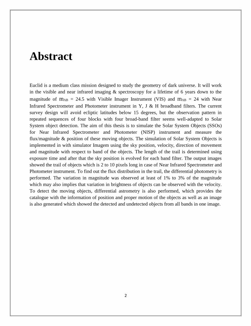
Euclid is a medium class mission designed to study the geometry of dark universe. It will work
in the visible and near infrared imaging & spectroscopy for a lifetime of 6 years down to the
magnitude of mAB = 24.5 with Visible Imager Instrument (VIS) and mAB = 24 with Near
Infrared Spectrometer and Photometer instrument in Y, J & H broadband filters. The current
survey design will avoid ecliptic latitudes below 15 degrees, but the observation pattern in
repeated sequences of four blocks with four broad-band filter seems well-adapted to Solar
System object detection. The aim of this thesis is to simulate the Solar System Objects (SSOs)
for Near Infrared Spectrometer and Photometer (NISP) instrument and measure the
flux/magnitude & position of these moving objects. The simulation of Solar System Objects is
implemented in with simulator Imagem using the sky position, velocity, direction of movement
and magnitude with respect to band of the objects. The length of the trail is determined using
exposure time and after that the sky position is evolved for each band filter. The output images
showed the trail of objects which is 2 to 10 pixels long in case of Near Infrared Spectrometer and
Photometer instrument. To find out the flux distribution in the trail, the differential photometry is
performed. The variation in magnitude was observed at least of 1% to 3% of the magnitude
which may also implies that variation in brightness of objects can be observed with the velocity.
To detect the moving objects, differential astrometry is also performed, which provides the
catalogue with the information of position and proper motion of the objects as well as an image
is also generated which showed the detected and undetected objects from all bands in one image.
Page 5
3
Résumé
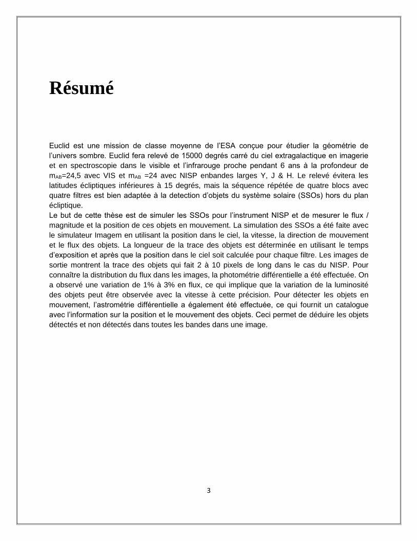
Euclid est une mission de classe moyenne de l’ESA conçue pour étudier la géométrie de
l’univers sombre. Euclid fera relevé de 15000 degrés carré du ciel extragalactique en imagerie
et en spectroscopie dans le visible et l’infrarouge proche pendant 6 ans à la profondeur de
mAB=24,5 avec VIS et mAB =24 avec NISP enbandes larges Y, J & H. Le relevé évitera les
latitudes écliptiques inférieures à 15 degrés, mais la séquence répétée de quatre blocs avec
quatre filtres est bien adaptée à la detection d’objets du système solaire (SSOs) hors du plan
écliptique.
Le but de cette thèse est de simuler les SSOs pour l’instrument NISP et de mesurer le flux /
magnitude et la position de ces objets en mouvement. La simulation des SSOs a été faite avec
le simulateur Imagem en utilisant la position dans le ciel, la vitesse, la direction de mouvement
et le flux des objets. La longueur de la trace des objets est déterminée en utilisant le temps
d’exposition et après que la position dans le ciel soit calculée pour chaque filtre. Les images de
sortie montrent la trace des objets qui fait 2 à 10 pixels de long dans le cas du NISP. Pour
connaître la distribution du flux dans les images, la photométrie différentielle a été effectuée. On
a observé une variation de 1% à 3% en flux, ce qui implique que la variation de la luminosité
des objets peut être observée avec la vitesse à cette précision. Pour détecter les objets en
mouvement, l’astrométrie différentielle a également été effectuée, ce qui fournit un catalogue
avec l’information sur la position et le mouvement des objets. Ceci permet de déduire les objets
détectés et non détectés dans toutes les bandes dans une image.
Page 6
4
Acknowledgements
I would like to thank my Supervisors Mr. Bruno Altieri and Mr. Luca Conversi from European
Space Astronomy Center (ESAC) for their valuable encouragement, support and monitoring
during the course of this internship/thesis. Each of them have been a wealth of useful information
and advice during this work as well as a source of inspiration for me and for my future. I am
truly lucky to have both of you as my supervisors and came up with topics that were exactly
what I wanted. I learned a lot from you and I am looking forward to work with you in future and
learn more science from you. I also want to thank the ESAC Euclid team for their help and
support.
Furthermore I would like thank my parents and brothers for their support throughout all my
study and encouraging me to pursue my education. Some special thanks to Véronique Chantrelle
and Sylvestre Maurice for helping me and motivating me towards my true passion and overall
played a big role in where I am today.
I also want to thank my fellow students & trainees for the fun and awesome times throughout the
last few years, be it either during leisure times or projects.
Finally, I am also thankful to everybody who was helpful and supportive for the success of this
internship and, I apologize to whom I could not mention one by one personally.
Page 7
5
Contents Abstract……………………………………………………………………………………………2
Acknowledgements………………………………………………………………………………..4
List of Figures……………………………………………………………………………………..7
List of Tables………………………………………………………………………………….......9
List of Abbreviations………………………………………………………………………….....10
1. Introduction……………………………………………………………………………………15
2. Euclid Mission………………………………………………………………………………...19
2.1 Euclid Science.......................................................................................................…...19
2.1.1 Primary Science……………………………………………………………22
2.1.1.1 Dark Energy……………………………………………………...22
2.1.1.2 Dark Matter……………………………………………………....23
2.1.1.3 Gravity Test……………………………………………………...23
2.1.1.4 Initial state of Universe…………………………………………..23
2.1.2 Legacy Science…………………………………………………………….24
2.2 Survey Design………………………………………………………………………..25
2.2.1 Wide Survey………………………………………………………………..25
2.2.2 Deep Survey………………………………………………………………..26
2.3 Ground Segment……………………………………………………………………..27
3. Scientific Instruments…………………………………………………………………………31
3.1 VIS Instrument……………………………………………………………………….33
Page 8
6
3.2 NISP Instrument……………………………………………………………………...34
3.2.1 Readout Principle…………………………………………………………..37
3.2.2 Near-Infrared Photometry Performance…………………………………...39
3.2.3 Near-Infrared Spectroscopy Performance………………………………….40
4. Solar system science with Euclid……………………………………………………………...42
4.1 Observation…………………………………………………………………………..42
4.2 Simulation……………………………………………………………………………44
4.2.1 Results and Discussion…………………………………………………….46
4.3 Photometry…………………………………………………………………………...47
4.3.1 Results and Discussion…………………………………………………….48
4.4 Astrometry…………………………………………………………………………...49
4.4.1 Results and Discussion…………………………………………………….51
Conclusion……………………………………………………………………………………….52
Appendices……………………………………………………………………………………….54
A. Configuration Files………………………………………………………………………54
B. Activities…………………………………………………………………………………64
C. Software flowchart……………………………………………………………………….66
Bibliography……………………………………………………………………………………..69
Page 9
7
List of Figures
1.1 Euclid Telescope. (Left) Design led by Astrium GmbH (Germany), (Right) Design led by
Thales Alenia Space Italy (Turin)………………………………………………………………..16
1.2 Cumulative size distribution of each SSO population……………………………………….18
2.1 (Left) Expansion history of universe and (Right) mass-energy budget at our cosmological
epoch ……………………...……………………………………………………………………..20
2.2 Two probes (Left) Weak Lensing (Right) Baryonic acoustic oscillation……………………21
2.3 The evolution of structure is seeded by quantum fluctuations amplified by inflation……….23
2.4 Euclid survey strategy………………………………………………………………………..25
2.5 Euclid Survey………………………………………………………………………………...26
2.6 Organisation of Science Data Centres (SDCs)………………………………………………27
2.7 Euclid data processing units………………………………………………………………….29
3.1 Schematic of resulting Optical design of Euclid……………………………………………..31
3.2 Mechanical Architecture of telescope………………………………………………………..32
3.3 NISP Instrument……………………………………………………………………………...34
3.4 NISP Optical design………………………………………………………………………….36
3.5 Wheel Mechanism: (a) Filter Wheel Assembly (FWA) & (b) Grism Wheel Assembly
(GWA)…………………………………………………………………………………………...37
3.6 Up the Ramp (UTR) Data Acquisition……………………………………………………....38
3.7 Bias of flux estimator………………………………………………………………………...39
3.8 The point spread functions…………………………………………………………………...40
3.9 Single chip H-band simulated Image………………………………………………………...40
3.10 Simulation of Euclid slitless observation…………………………………………………...41
Page 10
8
4.1 Euclid observation sequence…………………………………………………………………43
4.2 Euclid SSO observation trail…………………………………………………………………44
4.3 Overview of SSO catalogue………………………………………………………………….44
4.4 Simulation during (a) NIS (during VIS exposure), (b) Y exposure (c) J exposure, & (d) H
exposure………………………………………………………………………………………….47
4.5 Mosaic of Y band simulated images…………………………………………………………50
4.6 Detected sources overlap with reference sources……………………………………………51
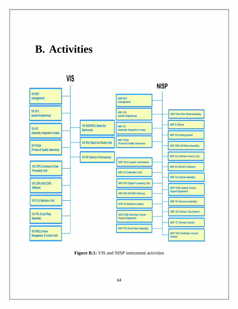
B.1 VIS and NISP instrument activities…………………………………………………………64
B.2 Science Ground Segment activities………………………………………………………….65
B.3 Science Working Groups……………………………………………………………………65
C.1 Flowchart of Imagem………………………………………………………………………..66
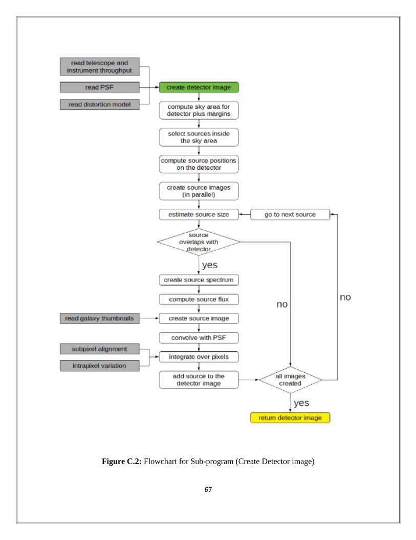
C.2 Flowchart for Sub-program (Create Detector image)……………………………………….67
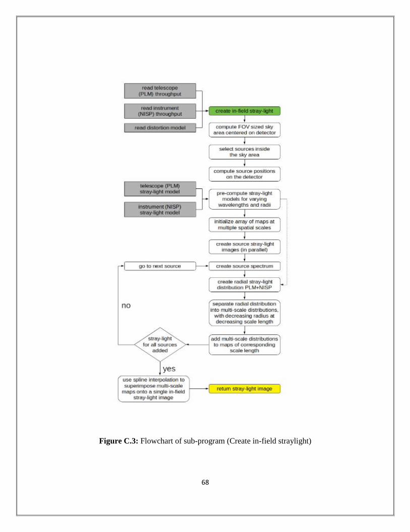
C.3 Flowchart of sub-program (Create in-field straylight)………………………………………68
Page 11
9
List of Tables
2.1 Euclid Performance based on survey………………………………………………………...24
2.2 Summary of Primary science………………………………………………………………...26
3.1 VIS Functional units’ description……………………………………………………………33
3.2 NISP main elements………………………………………………………………………….35
Page 12
10
List of Abbreviations
2MASS Two Micron All-Sky Survey
AU Astronomical Unit
AGN Active Galactic Nucleus
AOCS Attitude and Orbit Control System
ASCII American Standard Code for Information Interchange
BAO Baryonic Acoustic Oscillations
CCD Charge Coupled Devices
CDM Cold Dark Matter
CMB Cosmic Microwave Background
CR Cosmic Ray
CRFP Carbon Fiber Reinforced Plastic
CSD Cumulative Size Distribution
DDS Data Distribution System
DEC Declination
DENIS Survey Deep Near Infrared Survey of the Southern Sky
DES Dark Energy Survey
DHS Data Handling System
DUNE Dark UNiverse Explorer
EC SGS Euclid Consortium Science Ground Segment
ELA Euclid Legacy Archive
ELT Extremely Large Telescope
Page 13
11
EM Electromagnetic
EMA Euclid Mission Archives
eROSITA extended ROentgen Survey with an Imaging Telescope Array
ESA European Space Agency
ESO European Space Organisation for Astronomical Research in the
Southern Hemisphere
ESAC European Space Astronomy Centre
FITS Flexible Image Transport System
FoM Figure of Merit
FOV Field Of View
FPA Focal Plane Array
FWA Filter Wheel Assembly
FWHM Full Width at Half Maximum
GR General Relativity
GS Ground Segment
GWA Grism Wheel Assembly
HgCdTe Mercury Cadmium Telluride
HST Hubble Space Telescope
IMB Inner Main Belt
IOC Instrument Operation Center
IR Infra-red
ISO International Organization for Standardization
JWST James Webb Space Telescope
KBOs Kuiper-Belt Objects
LDAC Leiden Data Analysis Center
LSST Large Synoptic Survey Telescope
LTU Luleå Tekniska Universitet
Page 14
12
MACC Multi-Accumulation
MBA Main-Belt Asteroids
MCs Mars-Crossers
MMB Middle Main Belt
MOC Mission Operations Centre
Mpc Megaparsec
NEA Near-Earth Asteroids
NI-CU NISP Calibration Unit
NI-DCU NISP Detector Control Unit
NI-DPU NISP Data Processing Unit
NI-DS NISP Detector System
NI-FWA NISP Filter Wheel Assembly
NI-GWA NISP Grism Wheel Assembly
NI-ICU NISP Instrument Control Unit
NI-OMA NISP Opto-Mechanical Assembly
NIP Near Infrared Imaging Photometer Channel
NIR Near Infrared
NIS Near Infrared Spectroscopic Channel
NISP Near Infrared Spectrometer and Photometer
NNO New Norcia
OGS Operations Ground Segment
OMB Outer Main Belt
OU Organization Unit
Pbit Petabits
PF Processing Functions
PSF Point Spread Function
PSU Power Supply Units
Page 15
13
RA Right Ascension
ROE Read Out Electronic Units
RMS Root Mean Square
SAOImage DS9 Smithsonian Astrophysical Observatory Image Deep Space 9
SCAMP Software for Calibrating AstroMetry and Photometry
SDCs Science Data Centres
SExtractor Source Extractor
SGS Science Ground Segment
SiC Silicon Carbide
SNR Signal to Noise Ratio
SOC Science Operations Centre
SPACE SPectroscopic All Sky Cosmic Explorer
SSO Solar System Object
TIME-OBS Time of Observation at which Catalogue created
TTC Telemetry and Tele command
T_SIMULATION Time in which the Simulation/Observation takes places
UTR Up the Ramp
VIS VISible Imager
VISTA Visible and Infrared Survey Telescope for Astronomy
VI-CU VIS Calibration Unit
VI-CDPU VIS Control and Data Processing Unit
VI-FH VIS Flight Harness
VI-FPA VIS Focal Plane Assembly
VI-PMCU VIS Power and Mechanism Control Unit
VI-SU VIS Shutter
VLT Very Large Telescope
WCS World Coordinate System
Page 16
14
WISE Wide-field Infrared Survey Explorer
WL Weak Gravitational Lensing
WMAP Wilkinson Microwave Anisotropy Probe
Page 17
15
Chapter 1
INTRODUCTION
The more we know,
The more we know that we don’t know.
Socrates
Twinkling stars tempts everyone on Earth to see the sky and wonder about the universe and this
leads to monitor the sky to know more about space and time. Astronomy, in ancient times,
tracked the motion of the objects across the sky. As time passed & technology improved, the
distant regions of the universe have become accessible and revealing objects with fascinating
properties. We can now survey for new objects of the outer regions of our solar system including
tiny objects with their smaller satellites. However, there is a lot to learn about our solar system
itself.
The acceleration of the expansion universe is the biggest challenge of the cosmology, which is a
branch of astronomy and explain the origin and evolution of the universe from inflation & big
bang, and physics. The Euclid will observe and measure the shapes of the billions of galaxies &
redshifts of tens of millions of galaxies for weak lensing which will help to answer some
questions such as how cosmic acceleration, the velocity at which galaxy is receding from the
observer & continuously increasing with time causing expansion of the, modifies the expansion
and distribution of matter in the universe. The redshift defines the shift in light on wavelength
band coming from the objects in space and moving away from us. This redshift concept is the
key to record the expansion of the universe.
The nature of Dark matter and dark energy is still unknown but there are some observations that
are recorded by other missions will assist the Euclid’s work. In 2008, Fermi gamma-ray space
telescope was launched with one of the scientific goal to look at dark matter by probing excess
Page 18
16
gamma rays from Milky Way’s center and in 2014, NASA announced that the excess emission
seen in that area is consistent with some forms of dark matter. Other space mission whose
primary mission wasn’t to observe dark matter have glimpsed dark matter for example, in 2015,
data from the Hubble Space Telescope and the Chandra X-ray Observatory used to study the 72
galaxy cluster collisions. Using these observations results, it concluded that Astronomers can
map the distribution of dark matter by analyzing how the light from distant sources beyond the
cluster is magnified and distorted by gravitational effects. In 2013, ESA’s Gaia mission launched
to create the map of the stars position in sky most accurately. It is believed that charting their
movements will reveal more information about the nature of dark matter, and how it influenced
the universe's history.
For the first time, Euclid mission will provide homogeneous optical and NIR imaging and
spectroscopy survey for the entire extragalactic sky. Before Euclid, for whole sky optical survey,
different instruments were required at different hemisphere. Euclid will provide natural synergy
with other present & planned space based all sky surveys which also includes some other
missions such as Wide-field Infrared Survey Explorer (WISE), eROSITA and Planck/WMAP.
WISE can help in accurate determination of stellar masses and dust by providing additional
infrared fluxes on brightest Euclid sources. The eROSITA (extended ROentgen Survey with
an Imaging Telescope Array) will enhanced the studies cluster mass function. Plank/WMAP
(Wilkinson Microwave Anisotropy Probe) will provide the cross-correlations between these two
datasets looking for Cosmic Microwave Background (CMB) signals. The design of Euclid can be
seen in the Figure 1.1.
Figure 1.1: Euclid Telescope. (Left) Design led by Astrium GmbH (Germany). (Right) Design
led by Thales Alenia Space Italy (Turin)
Page 19
17
Euclid has synergy with large-mirror, smaller-area facilities like JWST, ELT, VLTs, etc. These
can provide detailed spectral information for the faint populations discovered by Euclid, as well
as their spectroscopic redshifts, important for calibrating Euclid’s photo-z at faint magnitudes.
The Euclid mission’s primary scientific goal is to understand the nature of dark energy & dark
matter by measuring weak gravitational lensing and galaxy clustering [Laureijs et al., 2011], but
also expected to carry out additional science. The solar system science is one of the legacy
science of Euclid. The Solar aspect angle of Euclid is determined as between 87 and 110 degrees
[B. Carry, 2017].
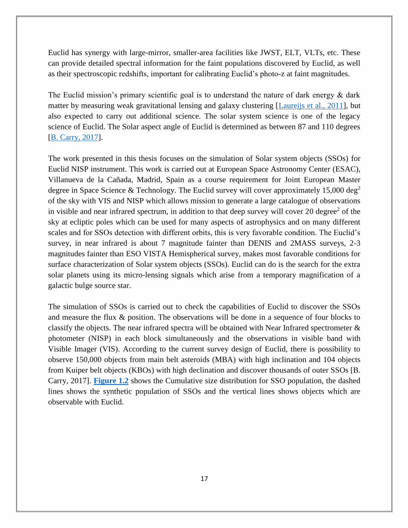
The work presented in this thesis focuses on the simulation of Solar system objects (SSOs) for
Euclid NISP instrument. This work is carried out at European Space Astronomy Center (ESAC),
Villanueva de la Cañada, Madrid, Spain as a course requirement for Joint European Master
degree in Space Science & Technology. The Euclid survey will cover approximately 15,000 deg2
of the sky with VIS and NISP which allows mission to generate a large catalogue of observations
in visible and near infrared spectrum, in addition to that deep survey will cover 20 degree2 of the
sky at ecliptic poles which can be used for many aspects of astrophysics and on many different
scales and for SSOs detection with different orbits, this is very favorable condition. The Euclid’s
survey, in near infrared is about 7 magnitude fainter than DENIS and 2MASS surveys, 2-3
magnitudes fainter than ESO VISTA Hemispherical survey, makes most favorable conditions for
surface characterization of Solar system objects (SSOs). Euclid can do is the search for the extra
solar planets using its micro-lensing signals which arise from a temporary magnification of a
galactic bulge source star.
The simulation of SSOs is carried out to check the capabilities of Euclid to discover the SSOs
and measure the flux & position. The observations will be done in a sequence of four blocks to
classify the objects. The near infrared spectra will be obtained with Near Infrared spectrometer &
photometer (NISP) in each block simultaneously and the observations in visible band with
Visible Imager (VIS). According to the current survey design of Euclid, there is possibility to
observe 150,000 objects from main belt asteroids (MBA) with high inclination and 104 objects
from Kuiper belt objects (KBOs) with high declination and discover thousands of outer SSOs [B.
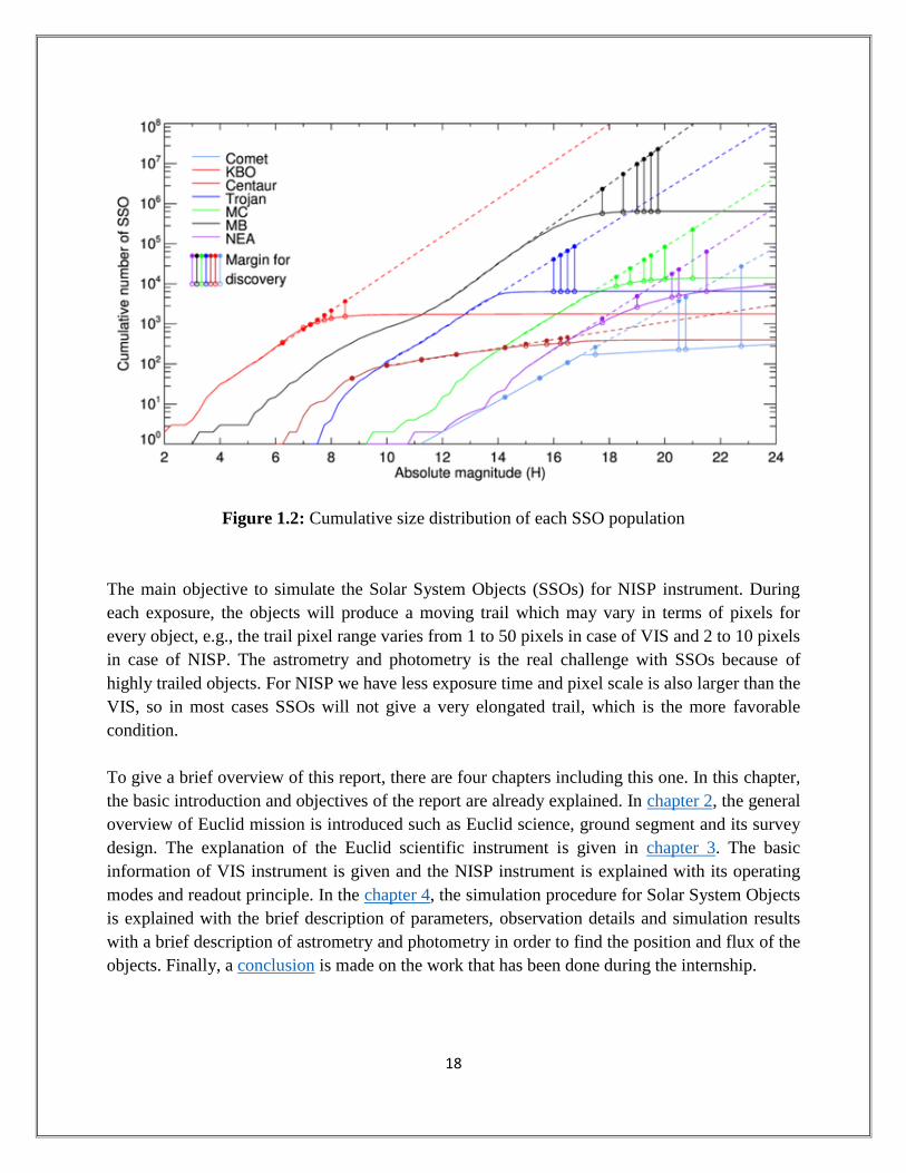
Carry, 2017]. Figure 1.2 shows the Cumulative size distribution for SSO population, the dashed
lines shows the synthetic population of SSOs and the vertical lines shows objects which are
observable with Euclid.
Page 20
18
Figure 1.2: Cumulative size distribution of each SSO population
The main objective to simulate the Solar System Objects (SSOs) for NISP instrument. During
each exposure, the objects will produce a moving trail which may vary in terms of pixels for
every object, e.g., the trail pixel range varies from 1 to 50 pixels in case of VIS and 2 to 10 pixels
in case of NISP. The astrometry and photometry is the real challenge with SSOs because of
highly trailed objects. For NISP we have less exposure time and pixel scale is also larger than the
VIS, so in most cases SSOs will not give a very elongated trail, which is the more favorable
condition.
To give a brief overview of this report, there are four chapters including this one. In this chapter,
the basic introduction and objectives of the report are already explained. In chapter 2, the general
overview of Euclid mission is introduced such as Euclid science, ground segment and its survey
design. The explanation of the Euclid scientific instrument is given in chapter 3. The basic
information of VIS instrument is given and the NISP instrument is explained with its operating
modes and readout principle. In the chapter 4, the simulation procedure for Solar System Objects
is explained with the brief description of parameters, observation details and simulation results
with a brief description of astrometry and photometry in order to find the position and flux of the
objects. Finally, a conclusion is made on the work that has been done during the internship.
Page 21
19
Chapter 2
EUCLID MISSION
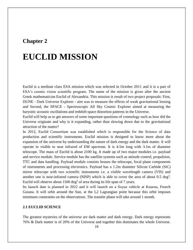
Euclid is a medium class ESA mission which was selected in October 2011 and it is a part of
ESA’s cosmic vision scientific program. The name of the mission is given after the ancient
Greek mathematician Euclid of Alexandria. This mission is result of two project proposals: First,
DUNE - Dark Universe Explorer - aim was to measure the effects of weak gravitational lensing
and Second, the SPACE - Spectroscopic All Sky Cosmic Explorer aimed at measuring the
baryonic acoustic oscillations and redshift-space distortion patterns in the Universe.
Euclid will help us to get answers of some important questions of cosmology such as how did the
Universe originate and why is it expanding, rather than slowing down due to the gravitational
attraction of the matter?
In 2012, Euclid Consortium was established which is responsible for the Science of data
production and scientific instruments. Euclid mission is designed to know more about the
expansion of the universe by understanding the nature of dark energy and the dark matter. It will
operate in visible to near infrared of EM spectrum. It is 4.5m long with 3.1m of diameter
telescope. The mass of Euclid is about 2100 kg. It made up of two major modules i.e. payload
and service module. Service module has the satellite systems such as attitude control, propulsion,
TTC and data handling. Payload module consists houses the telescope, focal plane components
of instruments and processing electronics. Payload has a 1.2m diameter Silicon Carbide (SiC)
mirror telescope with two scientific instruments i.e. a visible wavelength camera (VIS) and
another one is near-infrared camera (NISP) which is able to cover the area of about 0.5 deg2.
Euclid will observe about 1500 deg2 of area during its life span of 7 years.
Its launch date is planned in 2022 and it will launch on a Soyuz vehicle at Kourou, French
Guiana. It will orbit around the Sun, at the L2 Lagrangian point because this orbit imposes
minimum constraints on the observations. The transfer phase will take around 1 month.
2.1 EUCLID SCIENCE
The greatest mysteries of the universe are dark matter and dark energy. Dark energy represents
76% & Dark matter is of 20% of the Universe and together this dominates the whole Universe.
Page 22
20
There is only 4% of universe is visible out of which we can see only some fraction of it. The
dark energy is the main reason of the expanding universe but the existence and energy scale is
unexplainable with our current knowledge of physics. The Dark matter is said to be exert
gravitational attraction but doesn’t emit any light like visible universe objects do but actual
nature of dark matter is unknown because the axion are plausible candidates for cold dark matter
and massive neutrons for hot dark matter. The possible solution is Einstein’s theory of General
Relativity.
Figure 2.1: (Left) Expansion history of universe (Credit: Euclid Assessment Study Report) and
(Right) mass-energy budget at our cosmological epoch
Euclid Telescope will show the darker universe to us. It will observe large number of galaxies
and monitor observational marks of the dark matter, dark energy and gravity to map the
geometry of the universe. It will get high-resolution images and spectra, and characterize this
dark matter and dark energy using techniques such as weak gravitational lenses and the
clustering of galaxies.
Euclid will measure galaxy redshift up to 2, hence with a large enough look-back time to study
Dark energy that causes the acceleration of the expansion of the Universe. As stated above,
Euclid is merging result of DUNE and SPACE. And both of these missions were designed to
study the dark matter and dark energy with two different methods/probes. Euclid is a high
precision mission which will use the two cosmological probes: Weak lensing and Baryonic
Acoustic Oscillations.
Page 23
21
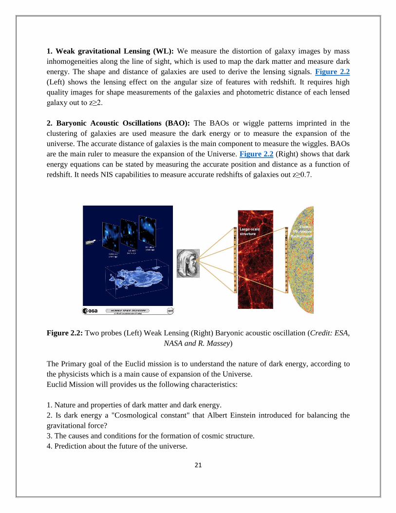
1. Weak gravitational Lensing (WL): We measure the distortion of galaxy images by mass
inhomogeneities along the line of sight, which is used to map the dark matter and measure dark
energy. The shape and distance of galaxies are used to derive the lensing signals. Figure 2.2
(Left) shows the lensing effect on the angular size of features with redshift. It requires high
quality images for shape measurements of the galaxies and photometric distance of each lensed
galaxy out to z≥2.
2. Baryonic Acoustic Oscillations (BAO): The BAOs or wiggle patterns imprinted in the
clustering of galaxies are used measure the dark energy or to measure the expansion of the
universe. The accurate distance of galaxies is the main component to measure the wiggles. BAOs
are the main ruler to measure the expansion of the Universe. Figure 2.2 (Right) shows that dark
energy equations can be stated by measuring the accurate position and distance as a function of
redshift. It needs NIS capabilities to measure accurate redshifts of galaxies out z≥0.7.
Figure 2.2: Two probes (Left) Weak Lensing (Right) Baryonic acoustic oscillation (Credit: ESA,
NASA and R. Massey)
The Primary goal of the Euclid mission is to understand the nature of dark energy, according to
the physicists which is a main cause of expansion of the Universe.
Euclid Mission will provides us the following characteristics:
1. Nature and properties of dark matter and dark energy.
2. Is dark energy a "Cosmological constant" that Albert Einstein introduced for balancing the
gravitational force?
3. The causes and conditions for the formation of cosmic structure.
4. Prediction about the future of the universe.
Page 24
22
In order to answer these questions, Euclid will be used to map the geometry of universe as a
function of redshift (0<z<2) or cosmological time (commonly used in big bang model).
2.1.1 Primary Science
In order to know the nature of dark energy and dark matter, the high precision measurements are
required and Euclid is designed to take the accurately measurements from space. Euclid mission
will create the largest map of the universe and trace the distribution of luminous as well as dark
components of the universe. Euclid will be able to answer the key questions about dark energy,
dark matter, gravity and initial state of universe.
1. Is the dark energy simply a cosmological constant, or is it a field that evolves
dynamically with the expansion of the Universe?
2. What is dark matter? What is the absolute neutrino mass scale and what is the number of
relativistic species in the Universe?
3. Alternatively, is the apparent acceleration instead a manifestation of a breakdown of
General Relativity on the largest scales, or a failure of the cosmological assumptions of
homogeneity and isotropy?
4. What is the power spectrum of primordial density fluctuations, which seeded large-scale
structure, and are they described by a Gaussian probability distribution?
2.1.1.1 Dark Energy
The ratio of the pressure to density of dark energy p (a) = w(a)×ρ(a)c2 is said to be dark energy
equation of state. The high precision redshift dependence of the function is one of the main goal
of Euclid mission which can be parameterized using first order Taylor expansion wrt the scale
factor a = 1/ (1+z), w(a)= wp + (ap−a) wa. The cosmological constant corresponds to w(a) = -1
imply a dynamical dark energy. An important question for Euclid is how to determine the w(a).
Currently, we can only present the statistical argument instead of theoretical guidance that w(a)
needs to be calculated as a precision ~1% to test the cosmological constant model. There is
possibility to compare two models of dark energy, one with cosmological constant and another
model where two parameters wp and wa varies with in a reasonable range. Cosmological constant
model would be favored and simpler for small variations but two parameter model will be
considered if variations are large. This quantified by Bayesian evidence calculation which shows
that cosmological constant model will be favored when data are consistent and FoM>400
(△wp~0.016 and △wa~0.16).
Page 25
23
2.1.1.2 Dark Matter
The total neutrino mass is the sum of the masses of the three known species (electron, muon and
tau neutrinos). Massive neutrinos damp structure growth on small scales. The larger the mass,
the more damping occurs, leaving a clear signature in the matter power spectrum observed by
Euclid.
2.1.1.3 Gravity Test
Einstein theory of general relativity (GR) is another possibility to explain the cosmic acceleration
and also understand the gravity so we can revise the cosmological scale. The expansion history,
evolution of perturbations and growth structure of the universe will change as models modify the
GR. The goal of the Euclid to measure the growth of structure with respect to canonical dark
energy models (γ) with a 1σ uncertainty of 0.02 then testing the general relativity with precision
so we can reconstruct the growth history in several redshift bins.
2.1.1.4 Initial State of Universe
To solve the number of problems in big bang cosmology using the large scale structure that
Euclid will observe arises from the quantum fluctuations that grew to cosmological scales during
inflation.
Inflation models can predict a primordial power spectrum scale invariant with power law spectral
index ns~1. Euclid will measure the spectral index with a precision similar to that of Planck, and
providing independent confirmation of the cosmic microwave background (CMB) results. Euclid
will improve the constraints on power spectrum of initial fluctuation by a factor 2 over Planck
alone.
Figure 2.3: The evolution of structure is seeded by quantum fluctuations amplified by inflation.
By combining Euclid and CMB data we will map the evolution of structure over orders of
magnitude in time.
Page 26
24
The concordance cosmological model assumes an initial Gaussian random field of perturbations,
from which large-scale structure grows. A detection of non-Gaussianity would signify a
departure from this central assumption of the current standard model. The fNL parameter is a way
to quantify the amplitude of this effect.
Table 2.1: Summary of Primary science
Science Targets
Dark Energy 1. Measure the expansion of universe with in the redshift bins
0.7<z<2.
Dark Matter 1. Detect dark matter halos on a mass scale between 108 and
>1015 MSun
2. Measure the dark matter mass profiles on cluster and galactic
scales
Gravity Test 1. Measure the growth index with a precision of 0.02 and the
growth rate in redshift bins between 0.5< z < 2.
2. Test the cosmological principle
Initial State of Universe 1. Measure the matter power spectrum on a large range of
scales
2. Measure a non-Gaussianity parameter: fNL for local-type
models with an error < +/-2.
2.1.2 Legacy Science
The current survey of Euclid covers approximately 15,000 deg2 of the sky with VIS and NISP
which allows mission to generate a dataset of observations in Visible and near Infrared spectrum
which can be used on many aspects of astrophysics and on many different scales such as
detection of SSOs, brown dwarfs.
In addition to that, the Deep survey which covers the 20 deg2 of the sky at ecliptic poles, is not
required only for calibration but also can be used for other science such as Type Ia Supernova
searches. If I say more briefly, Euclid will provide the more detailed study of thin and thick disk
of our galaxy using the deep survey. It would trace the spiral arms, extent of galactic bar, star
formation rates etc.
Another legacy science that Euclid can do is the search for the extra solar planets using its micro-
lensing signals which arise from a temporary magnification of a galactic bulge source star.
Euclid’s high angular resolution and VIS & NIR sensitivity will provide the detection of planets
down to 0.1-1 M⊕ from orbits of 0.5 AU and will also give us the knowledge of the nature of
planetary systems and their host stars which is necessary to get more information about
planet formation and habitability.
Page 27
25
2.2 SURVEY DESIGN
Euclid survey is designed to observe and understand the expansion of Universe. Its observations
will be carried out in step and share mode. It will measure about 0.5 degrees2 of the sky at a time,
NISP and VIS will share the field of view (FOV), imaging approximately 30 galaxies per square
arc-min with redshift z=1. It will observe 10-20 degree of long strip per day i.e. the patches of
about 400 degrees2 per month. Euclid will point in opposite direction after every 6 months to
take the observations of the other hemisphere. Euclid mission is designed to complete two
surveys: Wide Survey ensures the performance of the primary science and Deep Survey for
legacy science. The survey strategy mainly designed by wide survey requirement and the main
considerations are given below which is shown in Figure 2.4.
1. In the ecliptic plane, the sun-spacecraft line will move 1 degree per day.
2. The spacecraft forces the pointing direction to be perpendicular to the Sun-spacecraft axis
and maintaining the thermal stability.
Figure 2.4: Euclid survey strategy (Credit: ESA)
2.2.1 Wide Survey
Euclid will cover the darkest sky, free from our galaxy and solar system’s light, with 15,000
degress2 area. This is the core area to measure the Weak Lensing (WL), Baryonic Acoustic
Oscillations (BAO) and redshift signals. This survey will avoid the galactic latitudes (below 30
degree) and ecliptic latitudes (below 15 degree).
Page 28
26
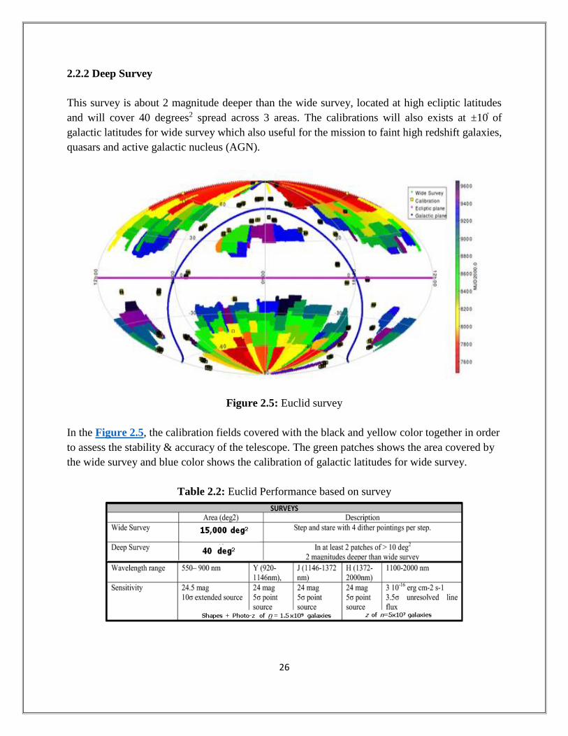
2.2.2 Deep Survey
This survey is about 2 magnitude deeper than the wide survey, located at high ecliptic latitudes
and will cover 40 degrees2 spread across 3 areas. The calibrations will also exists at ±10֯ of
galactic latitudes for wide survey which also useful for the mission to faint high redshift galaxies,
quasars and active galactic nucleus (AGN).
Figure 2.5: Euclid survey
In the Figure 2.5, the calibration fields covered with the black and yellow color together in order
to assess the stability & accuracy of the telescope. The green patches shows the area covered by
the wide survey and blue color shows the calibration of galactic latitudes for wide survey.
Table 2.2: Euclid Performance based on survey
Page 29
27
The hundreds of thousands of images and several tens of petabytes of data will be produced by
this complete survey. Billions of sources will be observed by Euclid which will be used for WL
and measuring galaxy redshifts.
2.3 GROUND SEGMENT
Euclid will deliver a large volume of data about 850 Gigabit of compressed data per day or 1 Pbit
data per year about 4 times more than Gaia. The data will be compressed by the Lossless
compression technique with compression rates of the order 2 to 3. The Euclid spacecraft will
perform the corrective actions on-board in case of any anomalies. The ground segment will not
need to monitor the spacecraft in real time.
The ground segment is composed of two units Science Operations Centre (SOC), and Science
Ground Segment (SGS) which are operated by the ESA and Euclid Consortium respectively. The
organization of SDCs is shown in figure. SOC will be the interface between ESA Mission
Operations Centre (MOC) and Euclid Operations Ground Segment (OGS). It will also manage
the downlink data with K-band and X-band tele-commanding and provide the data to SGS for
further science processing which will occur in national science data centers (SDCs).
Figure 2.6: Organization of Science Data Centers (SDCs) (Credit: ESA)
Page 30
28
MOC is located in ESOC, Darmstadt which will take care of mission operations planning,
execution, monitoring and controlling of spacecraft & ground segment. During Launch and Early
operations phase (LEOP), 3 Deep space antennas in New Norcia (NNO), Western Australia,
Cebreros (CEB), Spain and Malargue, Argentina will be used.
The SOC is located in ESAC, Villafranca del Castillo, Madrid, Spain which is in charge of the
scientific operations planning, monitor the performance and instrument files provided by MOC,
and interface with the Euclid Science Data Center (SDC) and archiving.
SGS is mainly responsible for the survey definition, data processing, and instrument operations
and archiving. SGS is designed to maximize the impact of Euclid. Ground based data from DES,
LSST and other optical surveys is used for the calibrations, quality control tasks, data reduction
and for photometric redshifts.
Data handling system is the main link between various branches of GS (MOC, SOC, IOCs and
SDCs) which is very cost effective and also avoid duplication of work and tasks. The data is
divided in to levels as follows:
1. Level 1: It includes the raw VIS and NISP images. Also unpacked & checked telemetry
data from satellite.
2. Level 2: This levels includes calibrated and intermediate data, PSF model and optical
distortion maps.
3. Level 3: It includes science ready data such as catalogues (including redshift, ellipticity,
shear, etc.), dark matter mass distribution and additional science catalogues. The level
two data is being processed to obtain the science goals of the mission using various
pipelines.
4. Level 4: This level includes data ready for public. This consists of level 3 data & some
part of level 2 data which combined together form Euclid legacy archive (ELA).
5. Level S (Simulation): This level includes pre-launch simulations and modelling data.
6. External Data: This data composed of re-processed data from existing mission & ground
based surveys which can be useful for simulation and calibration for the mission.
The data flows include:
MOC-SOC: The MOC sends telemetry data and attitude information to SOC via Data
Distribution System (DDS). SOC will send the tele-commands to plan the survey,
schedule the observations etc.
SOC-IOCs: The data flow of Level 1 data (all relevant instrument & science telemetry)
SDCs-IOCs: The data flow of simulated data.
IOC-IOC: The data flow of exchange of calibrated data between them.
IOCs-SDCs: The data flow of Level 2 and Level 3 data for science data processing.
Page 31
29
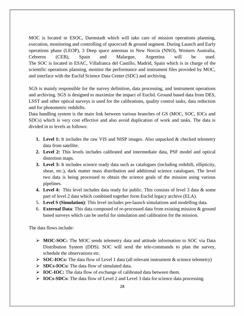
There are different data processing units and each level of data flows connected to these data
processing functions. The flow of data processing functions in the Euclid SGS is shown in
Figure 2.7 and briefly described below:
1. VIS: This function is for processing the Visible imaging data. It produces fully calibrated
images from edited telemetry to level 2.
2. NIR: It is in charge of processing the Near-Infrared imaging data. It also produces fully
calibrated images from edited telemetry to level 2 and allows spectra extraction.
3. SIR: It is in charge of processing the Near-Infrared imaging data. It also produces fully
calibrated images from edited telemetry to level 2 and extracts the spectra in the slitless
spectroscopic frames.
4. EXT: It is in charge for all the needed data to enter in Euclid Mission Archive (EMA) to
proceed with Euclid Science.
5. SIM: In order to test & validate the pipelines , this function implements the simulations.
6. MER: It merge all level 2 information and provides the stack images and source
catalogues.
7. SPE: It will extracts the Spectroscopic redshifts using the data and spectra from Level 2.
Figure 2.7: Euclid data processing units (Credit: Pasian F., et al.)
Page 32
30
8. PHZ: It will compute the photometric redshifts from the multi-wavelength imaging data.
9. SHE: It is going to compute the shape measurements on VIS data.
10. LE3: It computes all the high level science from the fully processed data.
Organisation unit (OU) supports each Processing functions (PF) inrequirements, algorithm and
prototype designs, test performances and comparision with requirements. One prototype get
validated by OU, it handed over to SDC, where this prototype is turned into a full-fledged Euclid
pipeline element.
Page 33
31
Chapter 3
SCIENTIFIC INSTRUMENTS
Euclid satellite is a 4.5m long X 3.1m in diameter and approximately 2100 kg of mass, consists
of a 1.2m diameter Korsch telescope to observe the universe with a large field of view (FOV).
The scientific goals described in previous chapter suggested a payload solution with two
instruments that is Visual Instrument (VIS) and Near Infrared Spectrometer and Photometer
(NISP) instrument and both instruments covers a large FOV of ~0.5degree2. The telescope
directs light to both instruments simultaneously using a dichroic filter in the exit pupil. The
reflected light is led to VIS and transmitted light goes to NISP. VIS will provide the high quality
images for doing processing for weak lensing galaxy shear measurements and NISP will perform
slitless spectroscopy to obtain spectroscopy redshifts and photometry to provide photometric
redshifts using near infrared (NIR) photometric measurements.
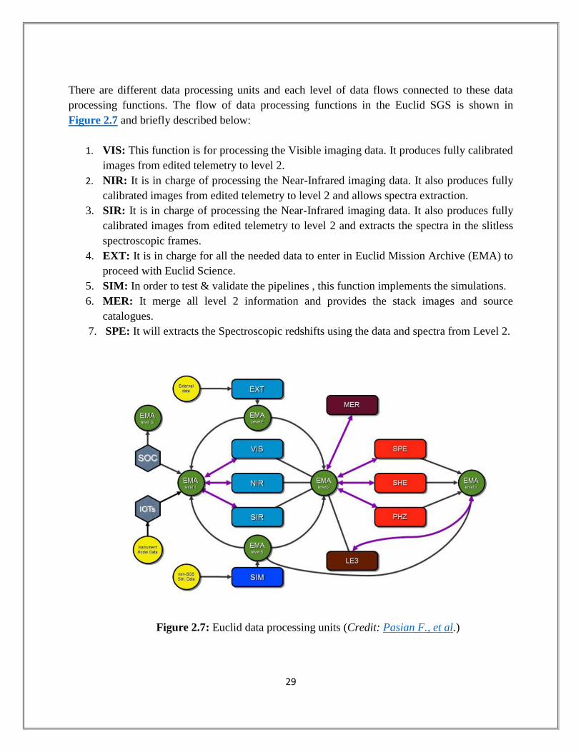
The main driving parameters to design the telescope is the high quality image from VIS for point
spread function’s (PSF) ellipticity, full width at half maximum (FWHM) and encircled energy.
According to the Euclid FOV, the two mirror telescope will not give a good image quality so the
three mirror configuration is the better solution for this problem such as Korsch configuration
because it provide more degree of freedom to get good level of image scale, aberration correction
and low distortion.
Figure 3.1: Schematic of resulting Optical design of Euclid
Page 34
32
Euclid telescope has three mirror Korsch configuration with 0.45 degree FOV and aperture stops
at primary mirror as shown in Figure 3.1. The entrance pupil diameter is 1.2m, the focal length
is 24.5m and FOV is 0.79m X 1.16 degree2. The interface between telescope & VIS and
telescope & NISP are focal plane & dichroic beam splitter respectively. The telescope directs
light to both instruments simultaneously using a dichroic filter in the exit pupil. The maximum
temperature of telescope is ~240K and NIR detector temperature should be ~100K in order to
minimize the dark current noise. VIS and NIP use a common M3 (mirror 3) optic.
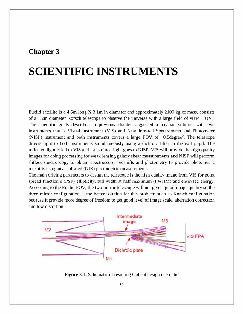
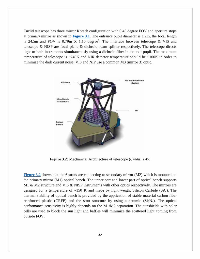
Figure 3.2: Mechanical Architecture of telescope (Credit: TAS)
Figure 3.2 shows that the 6 struts are connecting to secondary mirror (M2) which is mounted on
the primary mirror (M1) optical bench. The upper part and lower part of optical bench supports
M1 & M2 structure and VIS & NISP instruments with other optics respectively. The mirrors are
designed for a temperature of ~150 K and made by light weight Silicon Carbide (SiC). The
thermal stability of optical bench is provided by the application of stable material carbon fiber
reinforced plastic (CRFP) and the strut structure by using a ceramic (Si3N4). The optical
performance sensitivity is highly depends on the M1/M2 separation. The sunshields with solar
cells are used to block the sun light and baffles will minimize the scattered light coming from
outside FOV.
Page 35
33
3.1 VIS INSTRUMENT
It will be used for measuring gravitational lensing effects. It will study the dark matter
distribution. It will contains the 36 (array of 6 X 6) CCD based focal plane array (FPA) will
measure the shapes of galaxies with 0.1 arcsec pixels in 550-900 nm Passband (R+I+Z) &
resolution better than 0.18 arcsec. These CCDs have extremely high efficiency, low noise and
good radiation tolerance. Each CCD area have 4096 pixels X 4132 pixels, so the VIS will
generate 610 megapixel images.
The VIS channel is made up of some functional units and these are listed in the Table 3.1.
Table 3.1: VIS Functional units’ description
Name Unit Function Mass (Kg)
VI-FPA VIS Focal Plane Assembly Detection of visible light for
imaging
66
VI-SU VIS Shutter Close VIS optical path for read out
Close VIS optical path for dark
calibration
15
VI-CU VIS Calibration Unit Illumination the FPA with Flat field
for calibration
1
VI-
CDPU
Control and Data Processing
Unit
Control Instrument
Perform data processing
Interface with spacecraft for data
handling
17
VI-
PMCU
Power and Mechanism
Control Unit
Control units 14
The detector subassembly and the electronics sub-assembly together makes VIS Focal Plane
Assembly (VI-FPA) and these subassemblies are not linked mechanically but electrically by
CCD harnesses to prevent the mechanical and thermal perturbation. It is thermal-mechanical
structure which supports the detector assembly of 6X6 CCDs and provides path for power
dissipation by these CCDs to the radiator. It also associated with the Read out Electronic Units
(ROE) and Power supply units (PSUs).
VI-SU will prevent the CCDs from direct light falling when sensors are exposed to light
continuously.
VI-CU allows flat fields of focal plane array to be obtained. This unit will be driven by the VI-
PMCU.
VI-PMCU encompasses all the functions required to control VIS mechanisms as well as the
calibration sources.
Page 36
34
VI-CDPU is located in service module. It is responsible for the telemetry & tele-command
within the spacecraft control& data management unit, synchronizing all instrument activities,
instrument monitoring and control based on housekeeping data and data acquisition from ROEs
and processing based on telemetry command.
3.2 NISP INSTRUMENT
NISP (Near infrared spectrometer and photometer) instrument will operate in the range 0.9-2.0
micron of wavelength at temperature lower than 140K. It will be used to measure the redshifts of
the galaxies. Its spectroscopic data will explain the galaxy clusters and their distribution and then
the effects of the dark energy & dark matter over them. It has two modes of observations:
photometric mode and spectroscopic mode. The photometric mode will be used for the
acquisition of the images with broad band filters and the spectroscopic mode for the slitless
dispersed images on the detectors. NISP contains two channels slit-less spectrometer (NIS) and a
three band photometer (NIP). Both channels shares common optics, focal plane, electronics and
support structure. The overview of NISP can be shown in Figure 3.3.
Figure 3.3: NISP Overview
Page 37
35
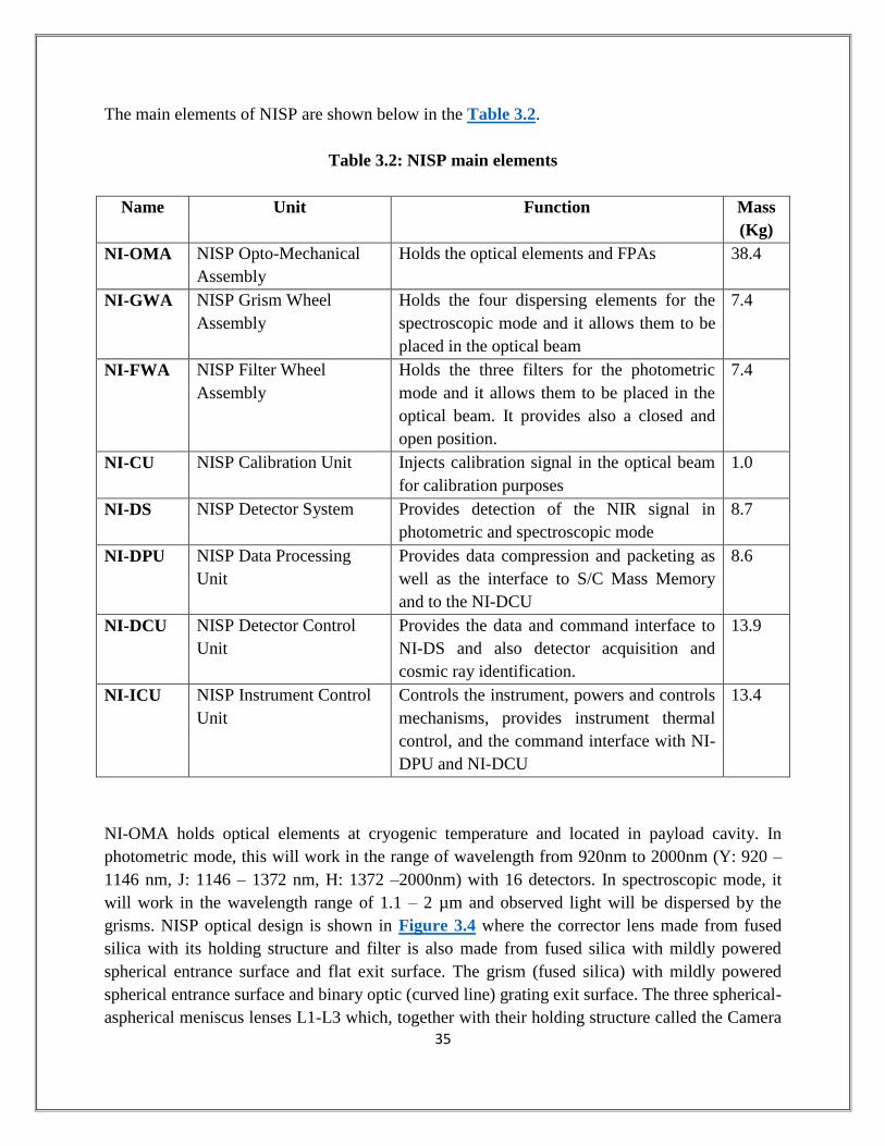
The main elements of NISP are shown below in the Table 3.2.
Table 3.2: NISP main elements
Name Unit Function Mass
(Kg)
NI-OMA NISP Opto-Mechanical
Assembly
Holds the optical elements and FPAs 38.4
NI-GWA NISP Grism Wheel
Assembly
Holds the four dispersing elements for the
spectroscopic mode and it allows them to be
placed in the optical beam
7.4
NI-FWA NISP Filter Wheel
Assembly
Holds the three filters for the photometric
mode and it allows them to be placed in the
optical beam. It provides also a closed and
open position.
7.4
NI-CU NISP Calibration Unit Injects calibration signal in the optical beam
for calibration purposes
1.0
NI-DS NISP Detector System Provides detection of the NIR signal in
photometric and spectroscopic mode
8.7
NI-DPU NISP Data Processing
Unit
Provides data compression and packeting as
well as the interface to S/C Mass Memory
and to the NI-DCU
8.6
NI-DCU NISP Detector Control
Unit
Provides the data and command interface to
NI-DS and also detector acquisition and
cosmic ray identification.
13.9
NI-ICU NISP Instrument Control
Unit
Controls the instrument, powers and controls
mechanisms, provides instrument thermal
control, and the command interface with NI-
DPU and NI-DCU
13.4
NI-OMA holds optical elements at cryogenic temperature and located in payload cavity. In
photometric mode, this will work in the range of wavelength from 920nm to 2000nm (Y: 920 –
1146 nm, J: 1146 – 1372 nm, H: 1372 –2000nm) with 16 detectors. In spectroscopic mode, it
will work in the wavelength range of 1.1 – 2 µm and observed light will be dispersed by the
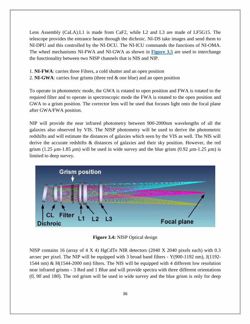
grisms. NISP optical design is shown in Figure 3.4 where the corrector lens made from fused
silica with its holding structure and filter is also made from fused silica with mildly powered
spherical entrance surface and flat exit surface. The grism (fused silica) with mildly powered
spherical entrance surface and binary optic (curved line) grating exit surface. The three spherical-
aspherical meniscus lenses L1-L3 which, together with their holding structure called the Camera
Page 38
36
Lens Assembly (CaLA).L1 is made from CaF2, while L2 and L3 are made of LF5G15. The
telescope provides the entrance beam through the dichroic. NI-DS take images and send them to
NI-DPU and this controlled by the NI-DCU. The NI-ICU commands the functions of NI-OMA.
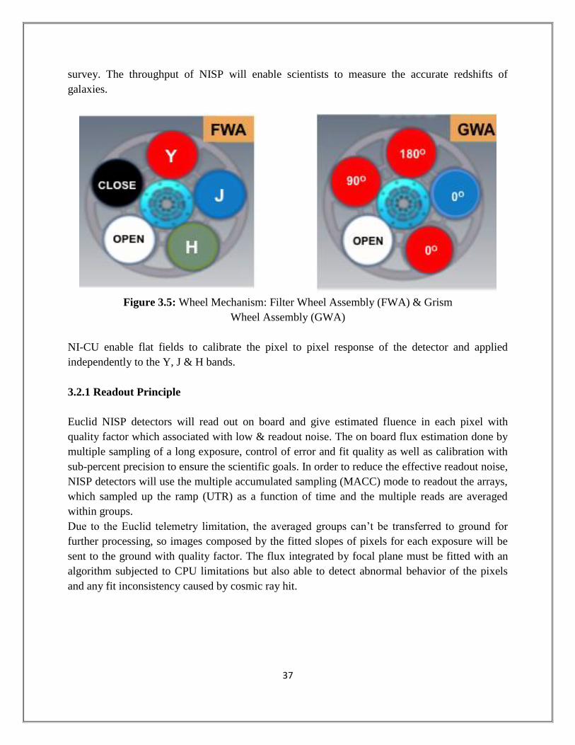
The wheel mechanisms NI-FWA and NI-GWA as shown in Figure 3.5 are used to interchange
the functionality between two NISP channels that is NIS and NIP.
1. NI-FWA: carries three Filters, a cold shutter and an open position
2. NI-GWA: carries four grisms (three red & one blue) and an open position
To operate in photometric mode, the GWA is rotated to open position and FWA is rotated to the
required filter and to operate in spectroscopic mode the FWA is rotated to the open position and
GWA to a grism position. The corrector lens will be used that focuses light onto the focal plane
after GWA/FWA position.
NIP will provide the near infrared photometry between 900-2000nm wavelengths of all the
galaxies also observed by VIS. The NISP photometry will be used to derive the photometric
redshifts and will estimate the distances of galaxies which seen by the VIS as well. The NIS will
derive the accurate redshifts & distances of galaxies and their sky position. However, the red
grism (1.25 µm-1.85 µm) will be used in wide survey and the blue grism (0.92 µm-1.25 µm) is
limited to deep survey.
Figure 3.4: NISP Optical design
NISP contains 16 (array of 4 X 4) HgCdTe NIR detectors (2040 X 2040 pixels each) with 0.3
arcsec per pixel. The NIP will be equipped with 3 broad band filters - Y(900-1192 nm), J(1192-
1544 nm) & H(1544-2000 nm) filters. The NIS will be equipped with 4 different low resolution
near infrared grisms - 3 Red and 1 Blue and will provide spectra with three different orientations
(0֯, 90 ֯ and 180 ֯). The red grism will be used in wide survey and the blue grism is only for deep
Page 39
37
survey. The throughput of NISP will enable scientists to measure the accurate redshifts of
galaxies.
Figure 3.5: Wheel Mechanism: Filter Wheel Assembly (FWA) & Grism
Wheel Assembly (GWA)
NI-CU enable flat fields to calibrate the pixel to pixel response of the detector and applied
independently to the Y, J & H bands.
3.2.1 Readout Principle
Euclid NISP detectors will read out on board and give estimated fluence in each pixel with
quality factor which associated with low & readout noise. The on board flux estimation done by
multiple sampling of a long exposure, control of error and fit quality as well as calibration with
sub-percent precision to ensure the scientific goals. In order to reduce the effective readout noise,
NISP detectors will use the multiple accumulated sampling (MACC) mode to readout the arrays,
which sampled up the ramp (UTR) as a function of time and the multiple reads are averaged
within groups.
Due to the Euclid telemetry limitation, the averaged groups can’t be transferred to ground for
further processing, so images composed by the fitted slopes of pixels for each exposure will be
sent to the ground with quality factor. The flux integrated by focal plane must be fitted with an
algorithm subjected to CPU limitations but also able to detect abnormal behavior of the pixels
and any fit inconsistency caused by cosmic ray hit.
Page 40
38
Figure 3.6: Up the Ramp (UTR) Data Acquisition
The abbreviation is used for this method is MACC (ng, nf, nd), where ng is the number of groups,
nf is the number of frames/group and nd is the number of frames that are dropped between two
successive groups. In each group, the frames are get averaged and then flux fitting is performed.
After frames averaging, the signal in group (Gk) is
Where, Si
(k) is the frame. This co-adding procedure helps to reduce Gaussian distributed pixel
readout noise.
During telemetry, image composed by the fitted slopes for each exposure is sent to the ground
using lossy compression.
As an example with the read outmode MACC (15, 16, 13) and pixel readout noise is 10 electron
rms proposed for NISP. The 10,000 nondestructive exposures with the input flux fin ranging from
0.1 e−1 s−1 to 150 e−1 s−1 are simulated. The signal accumulated between two successive groups
gin equals fintg = fin (nf + nd)tf , where tf = 1.3 s is the single frame read time and fe=1 e-1/ADU.
The accuracy of the flux estimator is tested by computing the bias.
The Figure 3.7 shows the results as a function of flux input, fin . The red bold solid line shows the
bias of the estimatorand green line shows the flux estimator.
Page 41
39
Figure 3.7: Bias of flux estimator
3.2.2 Near-Infrared Photometry (NIP) Performance
NIP mode will be used to get the photometric measurements in three (Y, J and H) bands. These
measurements along with the ground based multiband measurements will be used to estimate the
photometric redshift of the weak lensing galaxies. In order to complete the science requirements,
the imaging mode must have the depth of YAB, JAB and HAB = 24 mag (5σ) with high image
quality. To cover the 0.5 deg2 instrument FOV, 16 detectors are needed and the pixel scale is set
to the 0.3 ± 0.03 arcsec in order to reduce crowding.
The performance of NIP is briefly explained compared to two requirements: imaging quality and
depth requirements.
The optical performance of NISP imaging mode is evaluated by the constructing system. The
constructing system PSF is the combination of optical system PSF, generated by telescope &
instrument optical design perturbation, the satellite’s pointing jitter, provided by company as a
time series from ACS (Attitude Control System) simulations, and NISP PSF, from detector
effects. The imaging quality requirements of NISP are met for the system PSF, generated at focal
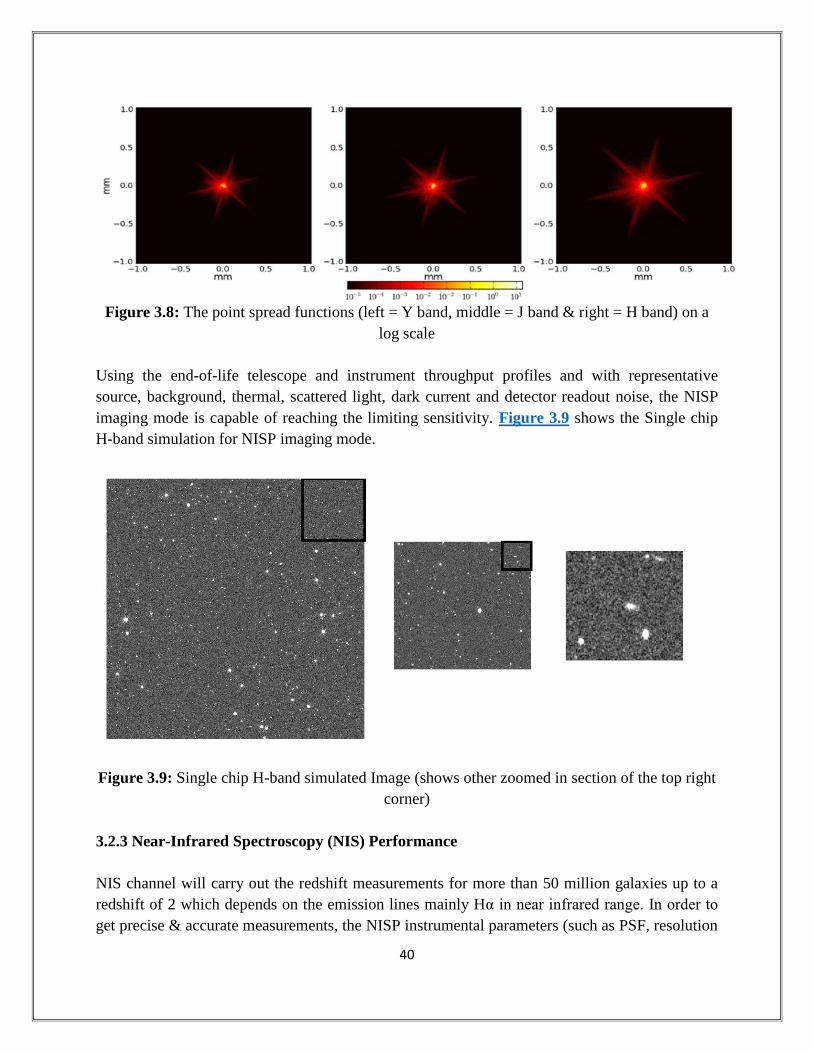
plane positions where the image quality was worst. The PSF for three bands is shown in Figure
3.8.
Page 42
40
Figure 3.8: The point spread functions (left = Y band, middle = J band & right = H band) on a
log scale
Using the end-of-life telescope and instrument throughput profiles and with representative
source, background, thermal, scattered light, dark current and detector readout noise, the NISP
imaging mode is capable of reaching the limiting sensitivity. Figure 3.9 shows the Single chip
H-band simulation for NISP imaging mode.
Figure 3.9: Single chip H-band simulated Image (shows other zoomed in section of the top right
corner)
3.2.3 Near-Infrared Spectroscopy (NIS) Performance
NIS channel will carry out the redshift measurements for more than 50 million galaxies up to a
redshift of 2 which depends on the emission lines mainly Hα in near infrared range. In order to
get precise & accurate measurements, the NISP instrumental parameters (such as PSF, resolution
Page 43
41
and instrumental background) and observation strategy should be considered to mitigate the
specific limitation of the slitless technique namely confusion.
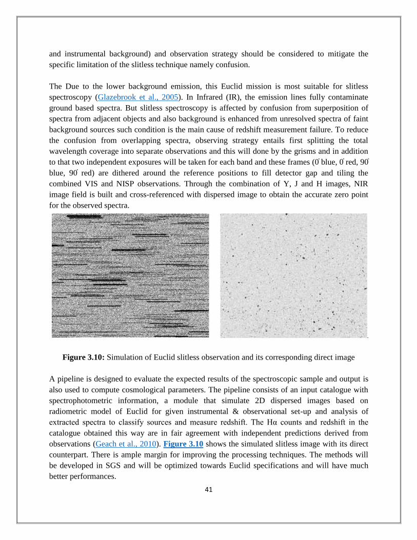
The Due to the lower background emission, this Euclid mission is most suitable for slitless
spectroscopy (Glazebrook et al., 2005). In Infrared (IR), the emission lines fully contaminate
ground based spectra. But slitless spectroscopy is affected by confusion from superposition of
spectra from adjacent objects and also background is enhanced from unresolved spectra of faint
background sources such condition is the main cause of redshift measurement failure. To reduce
the confusion from overlapping spectra, observing strategy entails first splitting the total
wavelength coverage into separate observations and this will done by the grisms and in addition
to that two independent exposures will be taken for each band and these frames (0 ֯ blue, 0 ֯ red, 90 ֯
blue, 90 ֯ red) are dithered around the reference positions to fill detector gap and tiling the
combined VIS and NISP observations. Through the combination of Y, J and H images, NIR
image field is built and cross-referenced with dispersed image to obtain the accurate zero point
for the observed spectra.
Figure 3.10: Simulation of Euclid slitless observation and its corresponding direct image
A pipeline is designed to evaluate the expected results of the spectroscopic sample and output is
also used to compute cosmological parameters. The pipeline consists of an input catalogue with
spectrophotometric information, a module that simulate 2D dispersed images based on
radiometric model of Euclid for given instrumental & observational set-up and analysis of
extracted spectra to classify sources and measure redshift. The Hα counts and redshift in the
catalogue obtained this way are in fair agreement with independent predictions derived from
observations (Geach et al., 2010). Figure 3.10 shows the simulated slitless image with its direct
counterpart. There is ample margin for improving the processing techniques. The methods will
be developed in SGS and will be optimized towards Euclid specifications and will have much
better performances.
Page 44
42
Chapter 4
SOLAR SYSTEM SCIENCE WITH
EUCLID
Euclid’s imaging and spectroscopic survey will carry out in visible and near infrared spectrum of
the extra-galactic sky of 15,000 deg2, and avoid galactic latitudes smaller than 30◦ and ecliptic
latitudes below 15◦ shown in Figure 2.2, totaling 35,000 pointings. The additional survey, two
magnitudes deeper and located at very high ecliptic latitudes, will cover 40 deg2 spread in three
areas. To monitor the stability of telescope PSF and assess the photometric and spectroscopic
accuracy, observation of calibration fields will be acquired which located at -10 ֯ and +10 ֯ of the
galactic latitude. Euclid has imaging detection limits of mAB = 24.5 (10σ on a 100 extended
source) with VIS, and mAB = 24 (5σ point source) with NISP. The NISP implementation consists
in two grisms, red and blue (as discussed in previous chapter), providing a continuum sensitivity
to mAB ≈ 21.
4.1 Observation
The Euclid pointing range is -3֯ towards +10 ֯ to observe orthogonally to the Sun. The observation
will be held in step-and-stare tiling mode and both instruments will target the same 0.57 degree2
field of view. Each tile will be visit once in wide survey and during deep survey it will be
pointed 40 times and 5 times in observation fields. Each observation will be done 16 times in an
hour in sequence of four observing blocks (Dithers) with a small step i.e. Dither step in between
the blocks which helps to maintain the focal plane of each instrument. In each block near
infrared slitless spectra will be obtained with NISP simultaneously with VIS image. Then images
will be taken with Y, J and H NISP filters as shown in Figure 4.1.
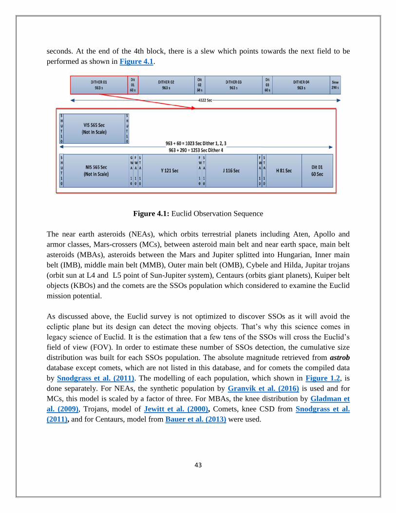
During each block VIS and NIS will work simultaneously with integration time of 565 seconds
and NIP will perform after VIS closes its shutter. The total block time of one dither is 963
Page 45
43
seconds. At the end of the 4th block, there is a slew which points towards the next field to be
performed as shown in Figure 4.1.
Figure 4.1: Euclid Observation Sequence
The near earth asteroids (NEAs), which orbits terrestrial planets including Aten, Apollo and
armor classes, Mars-crossers (MCs), between asteroid main belt and near earth space, main belt
asteroids (MBAs), asteroids between the Mars and Jupiter splitted into Hungarian, Inner main
belt (IMB), middle main belt (MMB), Outer main belt (OMB), Cybele and Hilda, Jupitar trojans
(orbit sun at L4 and L5 point of Sun-Jupiter system), Centaurs (orbits giant planets), Kuiper belt
objects (KBOs) and the comets are the SSOs population which considered to examine the Euclid
mission potential.
As discussed above, the Euclid survey is not optimized to discover SSOs as it will avoid the
ecliptic plane but its design can detect the moving objects. That’s why this science comes in
legacy science of Euclid. It is the estimation that a few tens of the SSOs will cross the Euclid’s
field of view (FOV). In order to estimate these number of SSOs detection, the cumulative size
distribution was built for each SSOs population. The absolute magnitude retrieved from astrob
database except comets, which are not listed in this database, and for comets the compiled data
by Snodgrass et al. (2011). The modelling of each population, which shown in Figure 1.2, is
done separately. For NEAs, the synthetic population by Granvik et al. (2016) is used and for
MCs, this model is scaled by a factor of three. For MBAs, the knee distribution by Gladman et
al. (2009), Trojans, model of Jewitt et al. (2000), Comets, knee CSD from Snodgrass et al.
(2011), and for Centaurs, model from Bauer et al. (2013) were used.
Page 46
44
According to the observation and pixel scale of the instruments, Euclid will be able to detect the
SSO using its trail appearance as shown in Figure 4.2 with speed greater than ≈ 0.2 arcsec per
hour.
Figure 4.2: Euclid SSO observation trail
4.2 Simulation
To simulate SSOs, the NISP simulator "Imagem" has been updated. The input for simulation of
SSOs with simulator Imagem is a unique catalogue which contains the following fields (shown
in Figure 4.3):
Figure 4.3: Overview of SSO catalogue
Page 47
45
i. (Ra0, Dec0): The coordinates of the SSOs for the first exposure and first dither of VIS
instrument.
ii. Velocity: The velocity of the SSOs with units in arcsec per hour.
iii. Theta: The movement of SSO in a particular direction with respect to the declination.
iv. Magnitude: The in-band magnitude of the objects for NISP it is Y_mag, J_mag and
H_mag for each band.
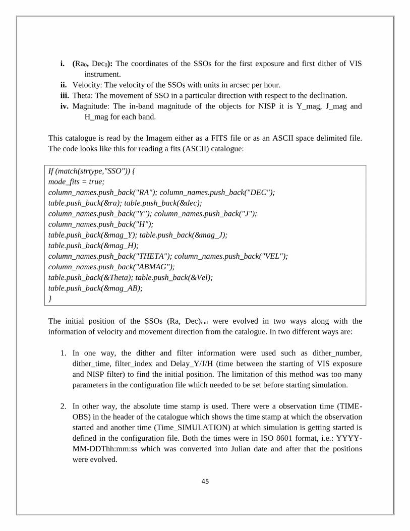
This catalogue is read by the Imagem either as a FITS file or as an ASCII space delimited file.
The code looks like this for reading a fits (ASCII) catalogue:
If (match(strtype,"SSO")) {
mode_fits = true;
column_names.push_back("RA"); column_names.push_back("DEC");
table.push_back(&ra); table.push_back(&dec);
column_names.push_back("Y"); column_names.push_back("J");
column_names.push_back("H");
table.push_back(&mag_Y); table.push_back(&mag_J);
table.push_back(&mag_H);
column_names.push_back("THETA"); column_names.push_back("VEL");
column_names.push_back("ABMAG");
table.push_back(&Theta); table.push_back(&Vel);
table.push_back(&mag_AB);
}
The initial position of the SSOs (Ra, Dec)init were evolved in two ways along with the
information of velocity and movement direction from the catalogue. In two different ways are:
1. In one way, the dither and filter information were used such as dither_number,
dither_time, filter_index and Delay_Y/J/H (time between the starting of VIS exposure
and NISP filter) to find the initial position. The limitation of this method was too many
parameters in the configuration file which needed to be set before starting simulation.
2. In other way, the absolute time stamp is used. There were a observation time (TIME-
OBS) in the header of the catalogue which shows the time stamp at which the observation
started and another time (Time_SIMULATION) at which simulation is getting started is
defined in the configuration file. Both the times were in ISO 8601 format, i.e.: YYYY-
MM-DDThh:mm:ss which was converted into Julian date and after that the positions
were evolved.
Page 48
46
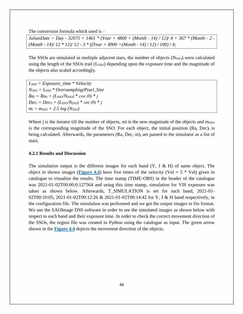
The conversion formula which used is –
JulianDate = Day - 32075 + 1461 * (Year + 4800 + (Month - 14) / 12)/ 4 + 367 * (Month - 2 -
(Month - 14)/ 12 * 12)/ 12 - 3 * ((Year + 4900 +(Month - 14) / 12) / 100) / 4;
The SSOs are simulated as multiple adjacent stars, the number of objects (NSSO) were calculated
using the length of the SSOs trail (LSSO) depending upon the exposure time and the magnitude of
the objects also scaled accordingly.
LSSO = Exposure_time * Velocity
NSSO = LSSO * Oversampling/Pixel_Size
Rai = Ra0 + (LSSO/NSSO) * cos (θ) * j
Deci = Dec0 + (LSSO/NSSO) * sin (θ) * j
mi = mSSO + 2.5 log (NSSO)
Where j is the iterator till the number of objects, mi is the new magnitude of the objects and mSSO
is the corresponding magnitude of the SSO. For each object, the initial position (Ra, Dec)i is
being calculated. Afterwards, the parameters (Ra, Dec, m)i are passed to the simulator as a list of
stars.
4.2.1 Results and Discussion
The simulation output is the different images for each band (Y, J & H) of same object. The
object in shown images (Figure 4.4) have five times of the velocity (Vel = 5 * Vel) given in
catalogue to visualize the results. The time stamp (TIME-OBS) in the header of the catalogue
was 2021-01-02T00:00:0.127564 and using this time stamp, simulation for VIS exposure was
taken as shown below. Afterwards, T_SIMULATION is set for each band, 2021-01-
02T00:10:05, 2021-01-02T00:12:26 & 2021-01-02T00:14:42 for Y, J & H band respectively, in
the configuration file. The simulation was performed and we got the output images in fits format.
We use the SAOImage DS9 software in order to see the simulated images as shown below with
respect to each band and their exposure time. In order to check the correct movement direction of
the SSOs, the region file was created in Python using the catalogue as input. The green arrow
shown in the Figure 4.4 depicts the movement direction of the objects.
Page 49
47
(a) (b)
(c) (d)
Figure 4.4: Simulation during (a) NIS (during VIS exposure), (b) Y exposure
(c) J exposure, & (d) H exposure
In the images, we can see the movement of the object as well as we can see that object is moving
in the direction as expected.
4.3 Photometry
Photometry is used to measure the intensity of the light of an object using EM radiation. It is
performed to calculate the output flux values for SSOs in a frame. This can be performed either
using aperture photometry or differential photometry.
In aperture photometry, the actual shape of source object is unknown or no assumption is made
by this technique. In this technique, the number of pixels are counted within the specified
aperture radius to provide the flux. As aperture radius is being increased the more flux from the
source also included as well as the noise from background included. In Differential photometry,
we compute the flux with respect to one or more sources. The objects were observed at same
spectral type or same brightness as comparison stars.
For photometry, the Astromatic software SExtractor (Source Extractor) is used. The SExtractor
first determines the background & its root mean square (RMS) noise and then check the pixels
Page 50
48
whether they belong to objects or background. The pixels above a certain threshold are
considered as objects pixel and then separately write down the properties of the objects in to a
catalogue. This catalogue, generated by SExtractor, is extracted using a series of parameters
which can be given in command line or in the configuration (.sex) file as an input file.
Commands -
Sex input_image -c configuration.sex
or
sex input_image1 input_image2 -c configuration.sex
or
sex input_image -c configuration.sex -Parameter_Name value . .
In second command line, first image is used to detect the position of the objects & second image
is used to do photometry. This is very convenient to use the series of images from different filters
with same aperture size. SExtractor uses the position information from the header but other
parameter (Mag_Zeropoint, Pixel_scale, Threshold etc) values should be provided by the user.
There is an option for filtering as well which smoothen the image & helps in detecting faint
object.
Another parameters known as deblending parameter which decide the adjacent pixels above
threshold is belongs to single object or to different objects. It is done by two parameters
DEBLEND_ NTHRESH and DEBLEND_NCOUNT which defines the number of levels
between threshold and maximum count in the object. After deblending, photometry is carried out
by the SExtractor. Gain & Mag_Zeropoint are the main parameters for photometry. Gain
converts count to the flux & Mag_Zeropoint calibrate the magnitude scale.
The Mag_Zeropoint were calculated using the formula -
m = -2.5 log(counts) + Mag_Zeropoint
Mag_Zeropoint may vary with time because of some factors such as dust deposition on mirror.
The parameters in output catalogue are choosen by user according to the requirement using the
file default.param.
4.3.1 Results and Discussion
During aperture photometry, the objects were moving and get trailed, so the magnitude
measurement was suffered from incorrect values and also created trailed PSF which is difficult to
approximate and cannot handled by SExtractor or any other publicly available software.
Page 51
49
SExtractor identified the point sources based on the parameter detection threshold which had
user-defined value in configuration file (default.sex).
During Differential photometry, the three stars were considered as reference and nearly with
same magnitude as of variable objects. Using SExtractor, the photometry is performed. The
observed variation in the magnitude was at most 1% to 3% of the magnitude which may implies
that variation in brightness can be observed with speed and rotation of object.
4.4 Astrometry
Astrometry detects the position and shift in the position of objects in the sky. In order to detect
the objects, first step is to compute the coordinates of each source on each image with respect to
the reference point. The Astromatic softwares SExtractor, SCAMP and SWARP are used to
create mosaic of frames, to register and calibrate images based on catalogs are used and then
derive the astrometric solution for our image.
SWARP created the stack of images or the mosaic of images based on the WCS which are re-
sampled as the program corrects for rotation and distortions. It is necessary to have all images
with same dimensions and the same observation time for each images. Swarp read the header of
input images one by one and check for contents. It built background images which get subtracted
from the images if necessary. Then images are re-sampled in order to provide a combined output
image. All parameter values for this process are used from the configuration file (config.swarp).
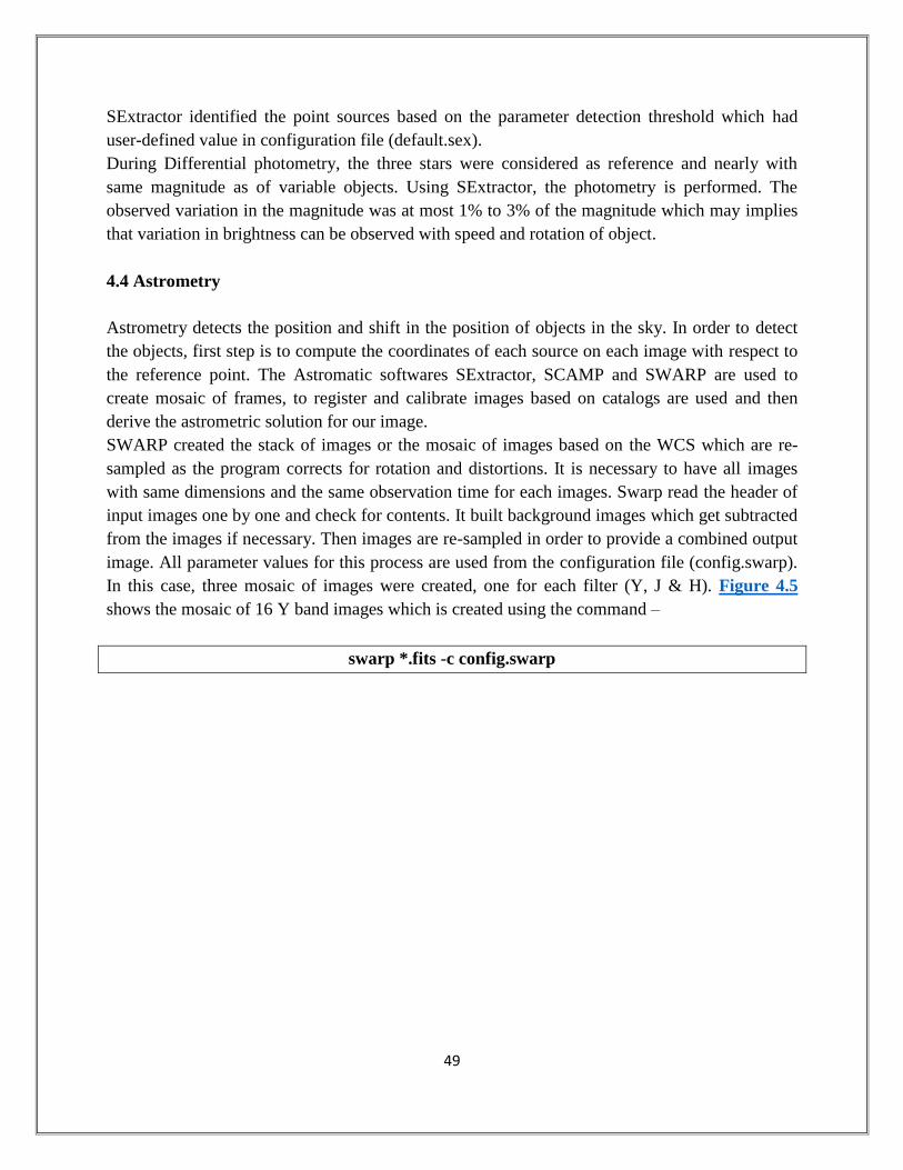
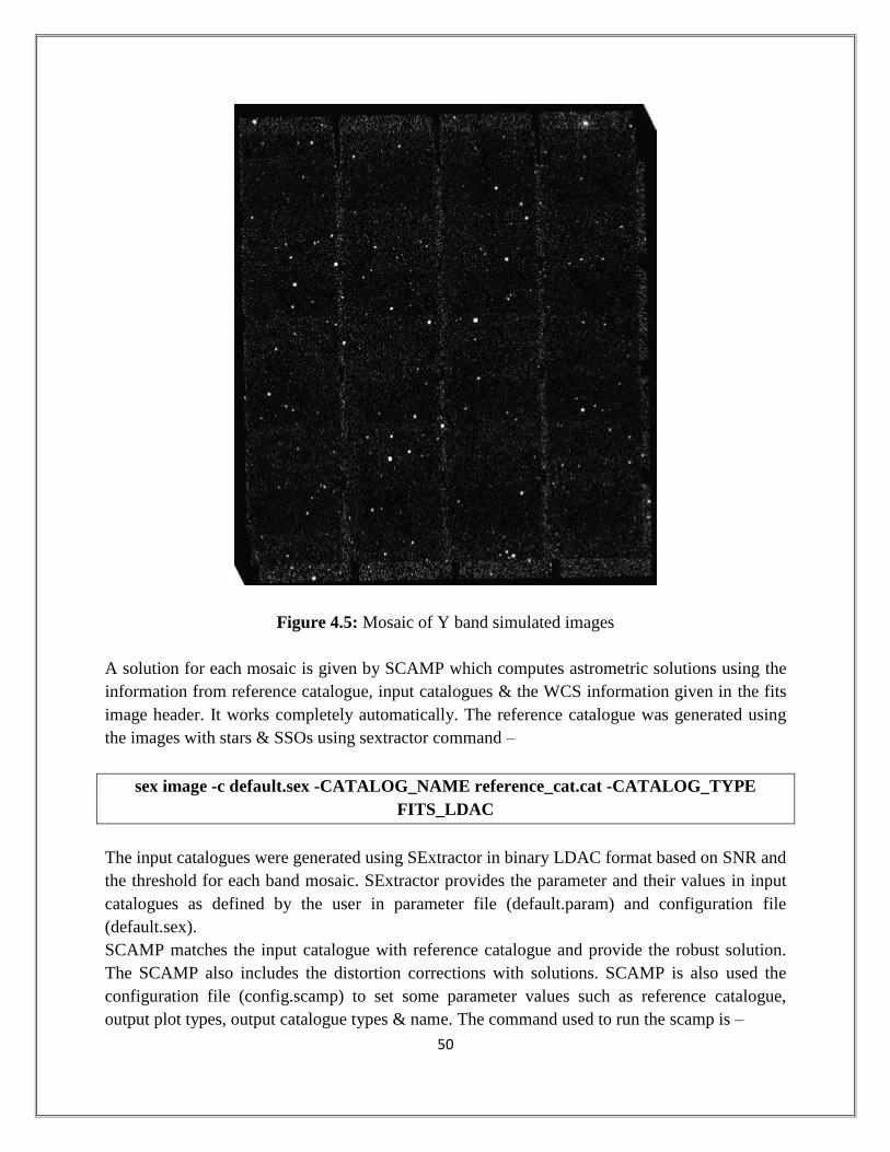
In this case, three mosaic of images were created, one for each filter (Y, J & H). Figure 4.5
shows the mosaic of 16 Y band images which is created using the command –
swarp *.fits -c config.swarp
Page 52
50
Figure 4.5: Mosaic of Y band simulated images
A solution for each mosaic is given by SCAMP which computes astrometric solutions using the
information from reference catalogue, input catalogues & the WCS information given in the fits
image header. It works completely automatically. The reference catalogue was generated using
the images with stars & SSOs using sextractor command –
sex image -c default.sex -CATALOG_NAME reference_cat.cat -CATALOG_TYPE
FITS_LDAC
The input catalogues were generated using SExtractor in binary LDAC format based on SNR and
the threshold for each band mosaic. SExtractor provides the parameter and their values in input
catalogues as defined by the user in parameter file (default.param) and configuration file
(default.sex).
SCAMP matches the input catalogue with reference catalogue and provide the robust solution.
The SCAMP also includes the distortion corrections with solutions. SCAMP is also used the
configuration file (config.scamp) to set some parameter values such as reference catalogue,
output plot types, output catalogue types & name. The command used to run the scamp is –
Page 53
51
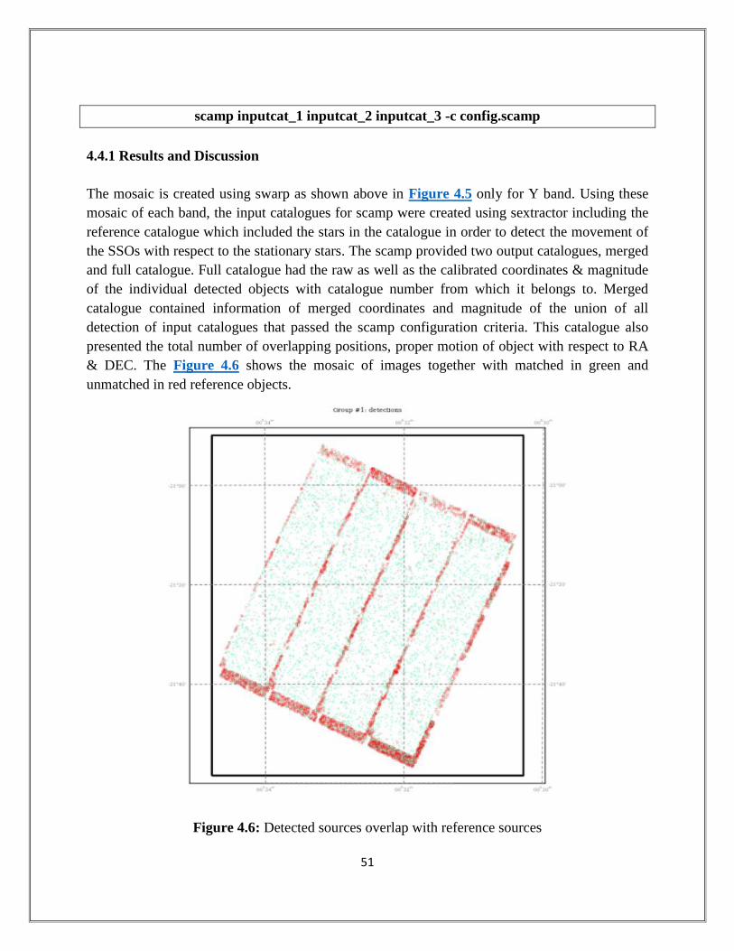
scamp inputcat_1 inputcat_2 inputcat_3 -c config.scamp
4.4.1 Results and Discussion
The mosaic is created using swarp as shown above in Figure 4.5 only for Y band. Using these
mosaic of each band, the input catalogues for scamp were created using sextractor including the
reference catalogue which included the stars in the catalogue in order to detect the movement of
the SSOs with respect to the stationary stars. The scamp provided two output catalogues, merged
and full catalogue. Full catalogue had the raw as well as the calibrated coordinates & magnitude
of the individual detected objects with catalogue number from which it belongs to. Merged
catalogue contained information of merged coordinates and magnitude of the union of all
detection of input catalogues that passed the scamp configuration criteria. This catalogue also
presented the total number of overlapping positions, proper motion of object with respect to RA
& DEC. The Figure 4.6 shows the mosaic of images together with matched in green and
unmatched in red reference objects.
Figure 4.6: Detected sources overlap with reference sources
Page 54
52
CONCLUSION
First, we have seen the contribution of ESA Euclid mission in solar system science and its
operating mode which will be able to detect and identify the moving objects. The large survey
design to cover about 15000 degree2 of sky and deep limiting magnitude (~24.5) of Euclid
promises to detect thousands of SSOs, even its survey will avoid the low ecliptic latitude, from
NEAs to KBOs including comets.
The main goal of this master thesis was to simulate the SSOs for NISP instrument of ESA Euclid
mission. This simulation was done to check the capabilities of Euclid for legacy science of solar
system. The simulation is done for three broadband filters Y, J and H with different exposure
time. The observation is carried out in a sequence of four blocks called dither. In each dither, the
four observations are taken by the instruments VIS and NISP spectroscopy simultaneously with
an integration time of 565 seconds and three NISP imaging exposure in a sequence which also
includes the overheads due to the FWA, GWA and shutter opening &/or closing. This simulation
was done using two methods and the generated output images from simulation using both
methods were same. In order to check the position and direction of movement of the objects, a
region file was generated using the input catalogue in python which gave the satisfactory results
when this uploaded over the output simulated images in DS9.
To measure the flux, the differential photometry was performed using Sextractor. The variation
in observed flux was about 1% to 3% of the flux which may be due to the trailed object. This
observation may implies that variation in brightness of objects can be observed with velocity and
rotation of object. To find out the moving objects and their position, differential astrometry was
performed using open source Swarp, Sextractor and Scamp astromatic softwares. The mosaic of
images for each band was used to create the catalogue of objects and also reference catalogue
was created which included the reference stationary stars with SSOs. After registering the input
catalogues and reference catalogue, the output catalogue was generated using scamp which
provided the information of the moving objects with their position & proper motion with respect
to the RA and DEC. This also generated an image of overlapping mosaics which showed the
detected objects with green color and also undetected objects with red color in all frames.
Page 55
53
The long sequence of the observation will be used to constrain the rotation period, spin
orientation and shape determination of SSOs along with the data of Gaia and LSST because the
spectral coverage of Euclid photometry (visible to near infrared spectrum) complements the
spectroscopy and photometry of Gaia and LSST (in visible spectrum) which can be used for
spectral classification. In order to get the exact number of SSOs, the data details have to be
refined which depends on the instrument characterization.
Furthermore, if there will be any extension in Euclid survey to lower latitude, it will increase the
number of SSOs and also will be helpful to study the already known dark matter of our solar
system.
Page 56
54
Appendices
A. Configuration Files
A.1 Sextractor.param
#------------------------------- Photometric Parameters ----------------------------
FLUX_AUTO #for SCAMP #Flux within a Kron-like elliptical aperture [count]
FLUXERR_AUTO #for SCAMP # RMS error for AUTO flux [count]
FLUX_APER # Flux vector within fixed circular aperture(s)
FLUXERR_APER # RMS error vector for aperture flux(es)
MAG_APER # Fixed aperture magnitude vector
MAGERR_APER # RMS error vector for fixed aperture mag.
#------------------------------- Position Parameters --------------------------------
X_IMAGE # Object position along x [pixel]
Y_IMAGE # Object position along y
XPEAK_WORLD
YPEAK_WORLD
X2_WORLD
Y2_WORLD
X_WORLD
Page 57
55
Y_WORLD
ERRA_WORLD
ERRB_WORLD
#------------------------------- Geometric Parameters -----------------------------
X2_IMAGE
Y2_IMAGE
XY_IMAGE
#------------------------------- Required by SCAMP -------------------------------
XWIN_IMAGE
YWIN_IMAGE
ERRAWIN_IMAGE
ERRBWIN_IMAGE
ERRTHETAWIN_IMAGE
#------------------------------- advised by SCAMP ----------------------------------
FLUX_RADIUS
FLAGS
A.2 default.sex
# Default configuration file for SExtractor 2.19.5
#-------------------------------- Catalog ------------------------------------
CATALOG_NAME out_cat.cat # name of the output catalog
CATALOG_TYPE FITS_LDAC # NONE, ASCII,ASCII_HEAD, or
# FITS_LDAC
Page 58
56
PARAMETERS_NAME Sextractor.param # name of the file containing catalog
#contents
#------------------------------- Extraction ----------------------------------
DETECT_TYPE CCD # CCD (linear) or PHOTO (with gamma
#correction)
DETECT_MINAREA 5 # min. # of pixels above threshold
DETECT_THRESH 2 # <sigmas> or <threshold>,<ZP> in mag.arcsec-2
ANALYSIS_THRESH 2 # <sigmas> or <threshold>,<ZP> in mag.arcsec-2
FILTER Y # apply filter for detection (Y or N)?
FILTER_NAME default.conv # name of the file containing the filter
DEBLEND_NTHRESH 32 # Number of deblending sub-thresholds
DEBLEND_MINCONT 0.005 # Minimum contrast parameter for deblending
CLEAN Y # Clean spurious detections? (Y or N)?
CLEAN_PARAM 1.0 # Cleaning efficiency
MASK_TYPE CORRECT # can be one of NONE, BLANK or CORRECT
#------------------------------ Photometry -----------------------------------
PHOT_APERTURES 5 # MAG_APER aperture diameter(s) in pixels
PHOT_AUTOPARAMS 2.5, 3.5 # MAG_AUTO parameters:
#<Kron_fact>,<min_radius>
PHOT_PETROPARAMS 2.0, 3.5 # MAG_PETRO parameters: <Petrosian_fact>,
#<min_radius>
SATUR_LEVEL 50000.0 # level (in ADUs) at which arises saturation
SATUR_KEY SATURATE # keyword for saturation level (in ADUs)
MAG_ZEROPOINT 29.8889 # (Y = 29.8889, J = 29.77383659, H = 29.7525)
MAG_GAMMA 4.0 # gamma of emulsion (for photographic scans)
GAIN 1.0 # detector gain in e-/ADU
Page 59
57
GAIN_KEY GAIN # keyword for detector gain in e-/ADU
PIXEL_SCALE 0.3 # size of pixel in arcsec (0=use FITS WCS info)
#------------------------- Star/Galaxy Separation ----------------------------
SEEING_FWHM 0.18 # stellar FWHM in arcsec
STARNNW_NAME default.nnw # Neural-Network_Weight table filename
#------------------------------ Background -----------------------------------
BACK_SIZE 64 # Background mesh: <size> or <width>,<height>
BACK_FILTERSIZE 3 # Background filter: <size> or <width>,<height>
BACKPHOTO_TYPE GLOBAL # can be GLOBAL or LOCAL
#------------------------------ Check Image ----------------------------------
CHECKIMAGE_TYPE OBJECTS # can be NONE, BACKGROUND,
#BACKGROUND_RMS, MINIBACKGROUND,
#MINIBACK_RMS, -BACKGROUND,
#FILTERED, OBJECTS, -OBJECTS,
#SEGMENTATION, or APERTURES
CHECKIMAGE_NAME check.fits # Filename for the check-image
A.3 config.swarp
#Default configuration file for SWarp 2.38.0
#----------------------------------- Output -----------------------------------
IMAGEOUT_NAME coadd.fits # Output filename
WEIGHTOUT_NAME coadd.weight.fits # Output weight-map filename
HEADER_SUFFIX .head # Filename extension for additional headers
Page 60
58
#------------------------------- Co-addition ----------------------------------
COMBINE Y # Combine resampled images (Y/N)?
COMBINE_TYPE MEDIAN # MEDIAN, AVERAGE, MIN, MAX, WEIGHTED
# CHI-OLD,CHI-MODE,CHI-MEAN,SUM,
# WEIGHTED_WEIGHT,MEDIAN_WEIGHT,
# AND,NAND,OR or NOR
CLIP_AMPFRAC 0.3 # Fraction of flux variation allowed with clipping
CLIP_SIGMA 4.0 # RMS error multiple variation allowed with clipping
CLIP_WRITELOG N # Write output file with coordinates of clipped pixels (Y/N)
CLIP_LOGNAME clipped.log # Name of output file with coordinates of clipped pixels
BLANK_BADPIXELS N # Set to 0 pixels having a weight of 0
#-------------------------------- Astrometry ----------------------------------
CELESTIAL_TYPE NATIVE # NATIVE, PIXEL, EQUATORIAL,
# GALACTIC, ECLIPTIC, or SUPERGALACTIC
PROJECTION_TYPE TAN # Any WCS projection code or NONE
PROJECTION_ERR 0.001 # Maximum projection error (in output pixels), or 0
#for no approximation
CENTER_TYPE ALL # MANUAL, ALL or MOST
PIXELSCALE_TYPE MEDIAN # MANUAL,FIT, MIN, MAX or MEDIAN
#-------------------------------- Resampling ----------------------------------
RESAMPLE Y # Resample input images (Y/N)?
RESAMPLE_DIR /home/vkansal # Directory path for resampled images
RESAMPLE_SUFFIX .resamp.fits # filename extension for resampled images
RESAMPLING_TYPE LANCZOS3 # NEAREST,BILINEAR,LANCZOS2,LANCZOS3
# LANCZOS4 (1 per axis) or FLAGS
INTERPOLATE Y # Interpolate bad input pixels (Y/N)?
Page 61
59
FSCALASTRO_TYPE FIXED # NONE,FIXED, or VARIABLE
SCALE_KEYWORD FLXSCALE # FITS keyword for the multiplicative factor
#applied to each input image
FSCALE_DEFAULT 1.0 # Default FSCALE value if not in header
GAIN_KEYWORD E_ADU # FITS keyword for effect. gain (e-/ADU)
GAIN_DEFAULT 1.0 # Default gain if no FITS keyword found 0 =
#infinity (all or for each image)
SATLEV_KEYWORD SATURATE # FITS keyword for saturation level (ADU)
SATLEV_DEFAULT 50000.0 # Default saturation if no FITS keyword
#--------------------------- Background subtraction ---------------------------
SUBTRACT_BACK Y # Subtraction sky background (Y/N)?
BACK_TYPE AUTO # AUTO or MANUAL
BACK_DEFAULT 0.0 # Default background value in MANUAL
BACK_SIZE 128 # Background mesh size (pixels)
BACK_FILTERSIZE 3 # Background map filter range (meshes)
BACK_FILTTHRESH 0.0 # Threshold above which the background-map
#filter operates
#------------------------------ Miscellaneous ---------------------------------
DELETE_TMPFILES Y # Delete temporary resampled FITS files(Y/N)?
COPY_KEYWORDS OBJECT # List of FITS keywords to propagate from the
#input to the output headers
VERBOSE_TYPE NORMAL # QUIET,LOG,NORMAL, or FULL
NNODES 1 # Number of nodes (for clusters)
NODE_INDEX 0 # Node index (for clusters)
NTHREADS 0 # Number of simultaneous threads for the SMP
#version of SWarp 0 = automatic
Page 62
60
NOPENFILES_MAX 512 # Maximum number of files opened by SWarp
A.4 config.scamp
# Configuration file
#----------------------------- Field grouping ---------------------------------
FGROUP_RADIUS 1.0 # Max dist (deg) between field groups
#---------------------------- Reference catalogs ------------------------------
ASTREF_CATALOG FILE # NONE, FILE, USNO-A1, USNO-A2,...
ASTREF_BAND DEFAULT # Photom. band for astr.ref.magnitudes or
#DEFAULT, BLUEST, or REDDEST
ASTREFCAT_NAME reference.cat # Local astrometric reference catalogs
ASTREFCENT_KEYS X_WORLD,Y_WORLD # Local ref.cat. centroid parameters
ASTREFERR_KEYS ERRA_WORLD,
ERRB_WORLD,
ERRTHETA_WORLD
ASTREFMAG_KEY
MAG_AUTO
# Local ref.cat. magnitude parameter
ASTREFMAGERR_KEY MAGERR_AUTO # Local ref.cat. mag. error parameter
ASTREFOBSDATE_KEY JD-OBS # Local ref.cat. obs. date parameter
ASTREFMAG_LIMITS -99.0,99.0 # Select magnitude range in
#ASTREF_BAND
SAVE_REFCATALOG Y # Save ref catalogs in FITS-LDAC format?
#--------------------------- Merged output catalogs ---------------------------
MERGEDOUTCAT_TYPE FITS_LDAC # NONE, ASCII_HEAD, ASCII,
#FITS_LDAC
Page 63
61
MERGEDOUTCAT_NAME merged.cat # Merged output catalog filename
#--------------------------- Full output catalogs ---------------------------
FULLOUTCAT_TYPE FITS_LDAC #NONE, ASCII_HEAD, ASCII, FITS_LDAC
FULLOUTCAT_NAME full.cat # Full output catalog filename
#----------------------------- Pattern matching -------------------------------
MATCH Y # Do pattern-matching (Y/N) ?
MATCH_NMAX 0 # Max.number of detections for MATCHing (0=auto)
PIXSCALE_MAXERR 1.2 # Max scale-factor uncertainty
POSANGLE_MAXERR 0.05 # Max position-angle uncertainty (deg)
POSITION_MAXERR 0.01 # Max positional uncertainty (arcmin)
MATCH_RESOL 0 # Matching resolution (arcsec); 0=auto
MATCH_FLIPPED N # Allow matching with flipped axes?
MOSAIC_TYPE FIX_FOCALPLANE #UNCHANGED, SAME_CRVAL,
#SHARE_PROJAXIS,
#FIX_FOCALPLANE or LOOSE
#---------------------------- Cross-identification ----------------------------
CROSSID_RADIUS 2.0 # Cross-id initial radius (arcsec)
#---------------------------- Astrometric solution ----------------------------
SOLVE_ASTROM Y # Compute astrometric solution (Y/N) ?
PROJECTION_TYPE SAME # SAME, TPV or TAN
ASTRINSTRU_KEY FILTER,QRUNID # FITS keyword(s) defining the astrom
STABILITY_TYPE INSTRUMENT #EXPOSURE, PRE-DISTORTED or
#INSTRUMENT
Page 64
62
CENTROID_KEYS XWIN_IMAGE,YWIN_IMAGE # Cat. parameters for
#centroiding
CENTROIDERR_KEYS
ERRAWIN_IMAGE,ERRBWIN_IMAGE,ERRTHETAWIN_IMAGE
# Cat. params for centroid err ellipse
DISTORT_KEYS XWIN_IMAGE,YWIN_IMAGE # Cat. parameters or FITS
#keywords
DISTORT_GROUPS 1,1 # Polynom group for each context key
DISTORT_DEGREES 3 # Polynom degree for each group
FOCDISTORT_DEGREE 1 # Polynom degree for focal plane coords
ASTREF_WEIGHT 1.0 # Relative weight of ref.astrom.cat
ASTRACCURACY_TYPE SIGMA-PIXEL # SIGMA-PIXEL, SIGMA-ARCSEC,
# or TURBULENCE-ARCSEC
ASTRACCURACY_KEY ASTRACCU # FITS keyword for ASTR_ACCURACY param.
ASTR_ACCURACY 0.0001 # Astrom. uncertainty floor parameter (pixels)
ASTRCLIP_NSIGMA 3.0 # Astrom. clipping threshold in sigmas
COMPUTE_PARALLAXES N # Compute trigonom. parallaxes (Y/N)?
COMPUTE_PROPERMOTIONS Y # Compute proper motions (Y/N)?
CORRECT_COLOURSHIFTS N # Correct for colour shifts (Y/N)?
INCLUDE_ASTREFCATALOG Y # Include ref.cat in prop.motions (Y/N)?
ASTR_FLAGSMASK 0x00fc # Astrometry rejection mask on SEx FLAGS
ASTR_IMAFLAGSMASK 0x0 # Astrometry rejection mask on IMAFLAGS
#------------------------------- Check-plots ----------------------------------
CHECKPLOT_CKEY SCAMPCOL # FITS keyword for PLPLOT field colour
CHECKPLOT_DEV PNG # NULL, XWIN, TK, PS, PSC, XFIG, PNG
CHECKPLOT_RES 0 # Check-plot resolution (0 = default)
CHECKPLOT_ANTIALIAS Y # Anti-aliasing using convert (Y/N) ?
Page 65
63
CHECKPLOT_TYPE FGROUPS
#------------------------------ Miscellaneous ---------------------------------
SN_THRESHOLDS 5.0,100.0 # S/N thresholds (in sigmas) for all and high-SN
#sample
FWHM_THRESHOLDS 0.0,100.0 # FWHM thresholds (in pixels) for sources
ELLIPTICITY_MAX 1 # Max. source ellipticity
FLAGS_MASK 0x00f0 # Global rejection mask on SEx FLAGS
WEIGHTFLAGS_MASK 0x00ff # Global rejec. mask on SEx FLAGS_WEIGHT
IMAFLAGS_MASK 0x0 # Global rejec. mask on SEx IMAFLAGS_ISO
Page 66
64
B. Activities
Figure B.1: VIS and NISP instrument activities
Page 67
65
Figure B.2: Science Ground Segment activities
Figure B.3: Science Working Groups
Page 68
66
C. Software Flowchart
Figure C.1: Flowchart of Imagem
Page 69
67
Figure C.2: Flowchart for Sub-program (Create Detector image)
Page 70
68
Figure C.3: Flowchart of sub-program (Create in-field straylight)
Page 71
69
BIBLIOGRAPHY
[1] A. Costille, et al. 2016, “Final design and choices for EUCLID NISP grism”, Proc. SPIE
9912, Space Telescopes and Instrumentation 2016: Optical, Infrared, and Millimeter Wave, 99
[2] B. Carry, 2017,”Solar system science with ESA Euclid”, ArXiv e-prints
[arXiv:1711.01342v1]
[3] B. Kubik, R. Barbier, E. Chabanat, et al. 2016, , “A New signal estimator from the NIR
Detectors of the Euclid Mission”, The Astronomical Society of the Pacific, 128:104504
[4] Bauer, J. M., Grav, T., Blauvelt, E., et al. 2013, Astrophysical Journal, 773, 22
[5] Epchtein, N., de Batz, B., Copet, E., et al. 1994, Astrophysics and Space Science, 217, 3
[6] Giuseppe D. Racca, et al. 2016,”The Euclid mission design”, ResearchGate,
publication/309283685
[7] Glazebrook, K., et al. 2005, New Astr. Rev. , 49, 374
[8] Geach, J.E., et al. ,2010, MNRAS 402,1330
[9] Granvik, M., Morbidelli, A., Jedicke, R., et al. 2016, Nature, 530, 303
[10] Gladman, B. J., Davis, D. R., Neese, C., et al. 2009, Icarus, 202, 104
[11] Jewitt, D. C., Trujillo, C. A., & Luu, J. X. 2000, Astronomical Journal, 120, 1140
[12] Laureijs, R., Amiaux, J., Arduini, S., et al. 2011,”Euclid Definition Study report”, ArXiv e-
prints [arXiv:1110.3193]
[13] McMahon, R. G., Banerji, M., Gonzalez, E., et al. 2013, The Messenger, 154, 35
[14] Pasian F., et al. 2012, “Science Ground Segment for the ESA Euclid mission”, Proc. SPIE
8451
[15] Skrutskie, M. F., Cutri, R. M., Stiening, R., et al. 2006, Astronomical Journal, 131, 1163
Page 72
70
[16] Snodgrass, C., Fitzsimmons, A., Lowry, S. C., & Weissman, P. 2011, Monthly Notices of
the Royal Astronomical Society, 414, 458
[17] Tereno I., et al. 2015, “Euclid Space Mission: building the sky survey”, ArXiv e-prints
[arXiv:1502.00903v1]
[18] Thierry Maciaszek, et al. 2016, “Euclid Near Infrared Spectrometer and Photometer
instrument concept and first test results obtained for different breadboards models at the end of
phase C”, Space Telescopes and Instrumentation 2016: Optical, Infrared, and Millimeter Wave
[19] http://sci.esa.int/euclid/
[20] http://www.ieec.cat/project/euclid/
[21] https://www.euclid-ec.org/