Simulation of the Economic Impact of Region-Wide Electricity Outages from A Natural Hazard Using a CGE Model 101 SIMULATION OF THE ECONOMIC IMPACT OF REGION-WIDE ELECTRICITY OUTAGES FROM A NATURAL HAZARD USING A CGE MODEL Gauri Shankar Guha, Arkansas State University ABSTRACT Analysis of economic losses from natural hazards assumes greater importance as societies expand, while extreme natural phenomena become more variable. The economic impact, of electricity outages resulting from an earthquake, has been simulated using a CGE model. The economic region is Memphis, Tennessee, which suffered the most powerful earthquake ever recorded in the US. Several sets of policy simulations are presented for a region-wide outage of electricity following an earthquake. These are further evaluated for different labor market assumptions and electricity price scenarios. Finally, a conditional systematic sensitivity analysis is carried out to test for parametric sensitivity of the results. Keywords: Natural hazards, economic impact estimation, CGE modeling. INTRODUCTION Analysis of Natural Hazard Impacts Economic impacts of natural hazards, like earthquakes, tornadoes, floods, etc. are the result of joint-interaction between extreme natural events and human activities (Kates, 1971). The ensuing devastation depends not only on the physical attributes of the event, like intensity, duration, spatial coverage etc., but also on the nature and density of economic activities in the region. Losses, however, extend beyond the directly visible damage. There are indirect economic losses from business disruption, due both to property damage as well as disruptions in supplies and utility lifelines. Reduced regional incomes can further dampen economic activity. In recent years, Computable General Equilibrium (CGE) Modeling has been extensively used for policy and environmental impact simulation both in developing and developed countries (Adkins and Garbaccio, 1999). Although there are few readily citable applications to natural hazards (see, e.g., Brookshire et al., 1997, Rose and Guha, 2004), it is argued that the CGE model is an appropriate technique because it simultaneously captures the multi-market, optimizing behaviors of producers and consumers, through the flexible specification of technology and preferences. This paper is motivated by the twin objectives of examining a region with a history of a major earthquake event, and that of employing a sophisticated modeling technique that can best portray ex poste economic adjustments. The study simulates the general equilibrium impact of electric lifeline disruptions, on the Shelby County (Memphis,
Transcript
Simulation of the Economic Impact of Region-Wide Electricity Outages from A Natural Hazard Using a CGE Model
101
SIMULATION OF THE ECONOMIC IMPACT OF REGION-WIDE ELECTRICITY OUTAGES FROM A NATURAL HAZARD USING A CGE MODEL Gauri Shankar Guha, Arkansas State University ABSTRACT Analysis of economic losses from natural hazards assumes greater importance as societies expand, while extreme natural phenomena become more variable. The economic impact, of electricity outages resulting from an earthquake, has been simulated using a CGE model. The economic region is Memphis, Tennessee, which suffered the most powerful earthquake ever recorded in the US. Several sets of policy simulations are presented for a region-wide outage of electricity following an earthquake. These are further evaluated for different labor market assumptions and electricity price scenarios. Finally, a conditional systematic sensitivity analysis is carried out to test for parametric sensitivity of the results. Keywords: Natural hazards, economic impact estimation, CGE modeling. INTRODUCTION Analysis of Natural Hazard Impacts Economic impacts of natural hazards, like earthquakes, tornadoes, floods, etc. are the result of joint-interaction between extreme natural events and human activities (Kates, 1971). The ensuing devastation depends not only on the physical attributes of the event, like intensity, duration, spatial coverage etc., but also on the nature and density of economic activities in the region. Losses, however, extend beyond the directly visible damage. There are indirect economic losses from business disruption, due both to property damage as well as disruptions in supplies and utility lifelines. Reduced regional incomes can further dampen economic activity. In recent years, Computable General Equilibrium (CGE) Modeling has been extensively used for policy and environmental impact simulation both in developing and developed countries (Adkins and Garbaccio, 1999). Although there are few readily citable applications to natural hazards (see, e.g., Brookshire et al., 1997, Rose and Guha, 2004), it is argued that the CGE model is an appropriate technique because it simultaneously captures the multi-market, optimizing behaviors of producers and consumers, through the flexible specification of technology and preferences. This paper is motivated by the twin objectives of examining a region with a history of a major earthquake event, and that of employing a sophisticated modeling technique that can best portray ex poste economic adjustments. The study simulates the general equilibrium impact of electric lifeline disruptions, on the Shelby County (Memphis,
Southwestern Economic Review
102
TN) regional economy, following a hypothetical earthquake, of 7.5M on the Richter scale. The Study Region In 1811-12, the New Madrid Seismic Zone located near Memphis, Tennessee witnessed the largest earthquake events in the U.S., all above 7 magnitude on the Richter scale, felt as far away as Quebec. Estimated losses were quite modest, because of sparse population density and low level of economic development (Shinozuka et al., 1998). However, such an event today could be very expensive in terms of human and economic losses. Memphis was founded in 1819 on the banks of the Mississippi River, soon after the major earthquake events, and quickly grew to become one of the largest cities in the US by the mid-19th century. It is now a city of 295 square miles, sitting on the intersection of several lifelines like oil and gas pipelines and electric gridlines, and houses close to 1 million people. It is a major market center for 6 southern states, particularly for cotton and tobacco trading, and an important hub for transportation and distribution (e.g., it is the FedEx headquarters). According to its website, the Memphis airport has been the number one cargo airport in the world since 1992. Economic Disruptions: Direct and Indirect Losses An earthquake affects an area in 2 ways that are amenable to measurement. Direct losses are evaluated in terms of repair and rehabilitation costs of property and lifelines, and constitute the primary estimates of the economic disaster (Shinozuka et al., 1998). Indirect losses result from the forward and backward linkages of business disruption and the cost of recovery. Lifelines, like electricity, water, communication, gas, sewage, etc., provide vital services that sustain an economy, just as neural or cardio-vascular networks sustain life within a human body (see, e.g., Brookshire et al., 1997, and Rose et al., 1997). Lifeline outages can cause production losses to otherwise unharmed local producers, as well as damage to far-flung productive entities that are not directly affected, but are economically linked to the units in the affected region. The total effect of an earthquake includes indirect losses caused by the disruption of urban lifelines and productive capital stock. A popular approach for estimating indirect losses is Input-Output (I-O) analysis, based on a static, linear model showing the transfers between sectors based on a given technology. It provides a strong framework for studying earthquake losses in a region, because it can show direct and indirect effects of any demand-side change based on the interdependencies in the I-O table. I-O models generate various multipliers that provide a simple mechanism for calculating indirect and induced effects. Mathematical (linear or non-linear) programming models using constrained optimization of affected resources provide the next step in the logical hierarchy of analysis (see, e.g., Cochrane et al., 1997, Cole, 1995, Rose et al., 1997). An important lacuna in the above approaches is that they ignore production and consumption non-linearities. Also, the economic importance of a single lifeline system is smothered by the noise of a system-wide comprehensive loss estimation. The point of departure of this research is that it isolates the impacts of a single lifeline system and estimates the general equilibrium effects of its outage. CGE models combine the advantages of both the I-O and LP approaches, because they reflect the
Simulation of the Economic Impact of Region-Wide Electricity Outages from A Natural Hazard Using a CGE Model
103
responsiveness, subject to resource constraints, of individual producers and consumers to price signals in a multi-market context (Brookshire et al., 1997, Rose and Guha, 2004). The CGE model, employed in this research, uses an estimate of electricity lifeline outages, derived from an engineering simulation to compute changes in economic variables across sectors vis-à-vis a benchmark economy. A general equilibrium solution is important both from the viewpoint of realizing the economic or shadow price of an uninterrupted service, and to provide a relevant basis for retrofitting and mitigation policies. METHODOLOGY CGE Modeling CGE modeling has emerged as a powerful workhorse for policy analysis ever since the 1950s, when it was shown that the concept of the Walrasian General Equilibrium could be brought under a computable framework (see, e.g., Shoven and Whalley, 1992). In recent years, it has been used extensively for tackling a variety of policy issues, with the rise of computation power. The CGE framework is a reasonably close simulation of the real economy, because it captures the net effect of changes in resource allocation by allowing the best selection amongst input and output choices available in different markets. In this sense, it offers a better perspective, compared to macro-econometric models, for testing the response of an economic system to quantifiable exogenous stimuli, especially when these responses represent a departure from historical circumstances. Hence, CGE was considered to be well suited for analyzing natural hazard issues (Rose and Guha, 2004). Advantages of the CGE model include flexibility in specifying technology and consumer preferences, use of prices to drive the changes in allocation, and an almost free choice of the level of sectoral disaggregation. CGE models also allow users to specify the nature of substitution between factor inputs on the supply side, and between imports and domestic supply on the demand side, by choosing appropriate functional forms. Essential Structure of a CGE model The standard implementation strategy is to simplify the CGE model as 4 blocks of non-linear equations that describe the functioning of an economy (see e.g., Rutherford, 1998). The supply side consists of price and quantity equations and production functions; the demand side has expenditure and equilibrium equations and utility functions; the income equations deal with value added to institutions; and finally there are closure rules which are system constraints or central balancing equations. Solving the CGE model entails the specification of closure conditions that refer to the balancing of major accounts in the economy – demand, supply, government and external sectors. The latter is of greater importance in regional CGEs as also in entire economies that are foreign-trade-intensive (see, e.g., Robinson et al., 1990). Income identities ensure consistency between institutional expenditures and values realized by the owners of resources. Closure rules balance the economy-wide
Southwestern Economic Review
104
endowments with the allocation of goods and services across various markets and ensure that the model conforms to Walras' Law of zero excess demand. In view of the available software solutions (“solvers”), an emerging trend is to formulate the CGE model as a mixed complementarity problem (MCP). This requires the equilibrium over 3 classes of central conditions, namely: zero-profit, market clearance and income balance (Markusen, 1997). The application model in this paper has been implemented as an MCP, using an MPSGE/GAMS solver. Zero-profit Constraints No producer earns an economic profit,
( )∏ ≥−=−j
jj pRpCp 0)()( for all j
where, ∏j
o)( is the unit profit function
and,
=≡ ∑
ijiij ygyppR 1)(|max)(
and,
=≡ ∑ 1)(|min)( xfxppC j
iiij is the cost function
(subscripts i, j denote goods, while f, g stand for production functions) Market Clearance Conditions These conditions stipulate that there is no excess demand in the market. This implies that equilibrium prices are both cause and effect of supply being at least equal to demand:
∑ ∑ ∑
∏≥+
∂
∂
j h hhhihi
i
jj Mpdw
p
py ),(
)(
,,
where, w is the endowments of resource i available to any institutional owner, and, the subscript h denotes households and other institutions generating final demand. The final demand function is derived from a standard utility maximization problem given a utility function and budget constraints. Income Balance In a general equilibrium, the incomes of resource owners must equal the market value of their resource endowments:
( )∑=i
hiih wpM ,
where, p is a non-negative n-vector of prices for all commodities; y is a non-negative m-vector of CRS production activities; and M is an h-vector of incomes of all institutions.
Simulation of the Economic Impact of Region-Wide Electricity Outages from A Natural Hazard Using a CGE Model
105
The Shelby County CGE (SCCGE) Model A CGE model, representing the Memphis economy, based on the data of Shelby County, Tennessee, has been developed using the structural considerations discussed below. Market Conditions Markets are assumed to be competitive both for factors and outputs. Prices are not sticky, viz. they are allowed to move both up and down, based on market forces. Also, the region has an open-economy, thus allowing free trade flows, and is a price-taker, a "small-country" assumption, implying that its market activities do not affect border prices. Demand-Side Assumptions The model recognizes 3 classes of consumers: low, medium and high-income earners. The consumer preferences have been represented by a Cobb-Douglas Utility Function:
∏i
iiX α where iα are the expenditure shares, and 1=∑
iiα
There are alternate hypotheses about how consumers choose between domestic and foreign supply. The "strong" Heckscher-Ohlin approach treats imports and domestic products as homogenous, and hence perfectly substitutable; while another approach treats these as "complementary". The Armington assumption of imperfect substitutability between goods “distinguished by place of production” has been employed because it is a reasonable solution to accounting problems such as that of "cross-hauling". Supply-Side Assumptions The technology of the region is assumed to be flexible, in the sense that it allows for factor substitution based on prices, and stable, meaning that there are no short-term changes or innovations. Factor endowments are finite and fixed within the region, but may be mobile across sectors. The production structure is hierarchical, implying that the substitution possibilities between factors of production are different depending upon the layer of aggregation. This includes an inherent assumption of homothetic weak separability, which stipulates that the optimum mix of sub-aggregates is independent of the factor mix at higher levels of aggregation. The CES functional form has been chosen to specify the supply block since it enjoys these qualities:
)1/(/)1(/1
−−
∑
σσσσσα
iii X
where, iα are factor shares, ( 1/1 =∑i
iσα ); iσ are substitution elasticities; Xi are
factors.
Southwestern Economic Review
106
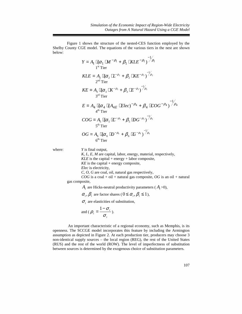
Figure 1 SCCGE Model – nesting structure of the CES production functions
Top Tier (KLEM) Production of the final product (Y), by combining materials (M) with a composite factor KLE. Second Tier (KLE) Production of the composite factor KLE, by combining labor (L) with a composite factor KE. Third Tier (KE) Production of the composite factor KE, through capital (K) – energy (E) substitution. Fourth Tier (E) Production of the energy composite E, by combining electricity (Elec) with an energy sub-aggregate (COG). Fifth Tier (COG) Production of the energy sub-aggregate COG, by combining coal (C) with an oil and gas composite (OG) Sixth Tier (OG) Production of the oil and gas composite OG, by combining oil (O) with natural gas (G)
KLE M
KE L
K E
Elec COG
Coal OG
Oil Gas
Y
Simulation of the Economic Impact of Region-Wide Electricity Outages from A Natural Hazard Using a CGE Model
107
Figure 1 shows the structure of the nested-CES function employed by the Shelby County CGE model. The equations of the various tiers in the nest are shown below:
1111
111 )( ρρρ βα−
−− ⋅+⋅⋅= KLEMAY 1st Tier
2221
222 )( ρρρ βα−
−− ⋅+⋅⋅= KELAKLE 2nd Tier
3331
333 )( ρρρ βα−
−− ⋅+⋅⋅= EKAKE 3rd Tier
4441
4444 ))(( ρρρ βα−
−− ⋅+⋅⋅⋅= COGElecAAE E 4th Tier
5551
555 )( ρρρ βα−
−− ⋅+⋅⋅= OGCACOG 5th Tier
6661
666 )( ρρρ βα−
−− ⋅+⋅⋅= GOAOG 6th Tier
where: Y is final output,
K, L, E, M are capital, labor, energy, material, respectively, KLE is the capital + energy + labor composite, KE is the capital + energy composite, Elec is electricity, C, O, G are coal, oil, natural gas respectively, COG is a coal + oil + natural gas composite, OG is an oil + natural
gas composite,
iA are Hicks-neutral productivity parameters ( iA >0),
ii βα , are factor shares ( 1,0 ≤≤ ii βα ),
iσ are elasticities of substitution,
and (i
ii σ
σρ −=
1).
An important characteristic of a regional economy, such as Memphis, is its openness. The SCCGE model incorporates this feature by including the Armington assumption as depicted in Figure 2. At each production tier, producers may choose 3 non-identical supply sources – the local region (REG), the rest of the United States (RUS) and the rest of the world (ROW). The level of imperfectness of substitution between sources is determined by the exogenous choice of substitution parameters.
Southwestern Economic Review
108
Figure 2 SCCGE Model – production nest with Armington conditions
KLE
Y
M
ROW
RUS
DOM
REG
K
E
Elec
ROW
REG
COG
Coal OG
Legend
Y = sectoral output KLE = capital+ labor,
energy aggregate M = materials K = capital E = energy bundle Elec = electricity COG = coal + oil +
gas aggregate OG = oil + gas bundle ROW = rest of world RUS = rest of the US REG = region DOM = REG + RUS
Oil Gas
RUS
RUS
RUS
REG REG
ROWROW
RUS
REG
ROW
Simulation of the Economic Impact of Region-Wide Electricity Outages from A Natural Hazard Using a CGE Model
109
Income Balance and Other Equilibrium Conditions Factor payments are distributed to households and institutions in the economy as labor and profit incomes. There are 2 levels of governments, Federal and State, that collect tax revenues and operate balanced budgets. Other equilibrium conditions include savings investment identity, balancing of the household budget and product and factor market clearance equations for all markets. Walras’ Law stipulates that the nth market clears automatically when (n-1) markets have cleared. At the operational level, it is important to recognize that including all n market equations would over-determine the model. Closure Rules Solving the CGE model entails balancing the demand and supply blocks and overcoming the problem of over-determination. This paper experiments with 2 of the common closure rules observed in the literature (Robinson et al., 1990, Dewatripont and Michel, 1987): the Keynesian closure which allows under-employment under a fixed wage rate regime, and the Neo-classical closure which forces full employment and variable wages. The Keynesian model is implemented by including fixed nominal wages and letting labor supply adjust, with no total labor use constraint. While the Neoclassical model is implemented by allowing wage rates to fluctuate and fixing labor supply by introducing a total labor constraint. MODEL IMPLEMENTATION Benchmark Data and Calibration The Input-Output (I-O) table gives a snapshot of economy wide transactions in a given year as a square matrix with economic sectors (industries and institutions) listed both as column and as row headers. Each column shows the activities of purchasers, and may be viewed as a “use” vector or a technology vector. Each row shows the activities of sellers, and may be regarded as a “make” or distribution vector. Any cell in an I-O table shows the amount of sector (row) i’s product used by sector (column) j. The I-O table of Shelby county appears in Table 1a. The Social Accounting Matrix (SAM) is an extension of the I-O table with an elaborate record of the institutional sectors. In a sense, the SAM is a system of bookkeeping for a “flow of funds” accounting of an entire economy by ensuring that total payments equal total receipts. The SAM is a systematic and extensive record of inter-industry, industry-institution and inter-institutional transfers, and forms the major database required to implement a CGE model. The other datasets required are:
1. Capital stock and Labor supply by economic sector in the region, 2. Constant elasticity of substitution (CES) / constant elasticity of
transformation (CET) values for the production and utility functions, and
3. Vector of counterfactual policy, externalities or stresses. These datasets are used to initialize exogenous parameters and calibrate the endogenous parameters of production and utility functions.
Southwestern Economic Review
110
Simulation of the Economic Impact of Region-Wide Electricity Outages from A Natural Hazard Using a CGE Model
111
Southwestern Economic Review
112
The SAM of the SCCGE model (shown in Table 1b) is derived from the 1996 release of Shelby county data from IMPLAN (MIG, 2000). The IMPLAN database reports the region's production information using a 528-industry classification. Following Rose and Benavides (1999), these have been aggregated into 20 sectors in the model, as shown in Table 2 below.
Table 2
Economic Sectors used in the Shelby County CGE Model
Sector Description Subsectors Output ($ million)
Employment (persons)
1 Agriculture 27 128 4,934
2 Mining 20 20 92
3 Construction 10 2,782 32,274
4 Food Processing 46 1,999 5,652
5 Manufactures 324 8,151 43,617
6 Petroleum Products 5 511 469
7 Transportation 9 6,235 56,151
8 Communication 2 654 2,953
9 Electricity 3 530 2,133
10 Gas Distribution 1 21 35
11 Water Supply and Sanitation 2 57 442
12 Wholesale Trade 1 4,581 41,293
13 Retail Trade 10 4,148 100,489
14 Finance Insurance and Real Estate (F.I.R.E.) 8 6,931 40,719
15 Personal Services 12 1,546 37,933
16 Business and Professional Services 21 3,917 85,814
17 Entertainment 7 293 6,395
18 Health 4 3,143 41,765
19 Education 5 1,324 37,083
20 Government 11 3,291 55,741
Total 528 50,263 595,986
Simulation of the Economic Impact of Region-Wide Electricity Outages from A Natural Hazard Using a CGE Model
113
Exogenous Parameters The SCCGE model employs a hierarchical CES function for describing sectoral production, because it allows for a flexible stage-wise substitution between sub-aggregates. The elasticity values used in this model reflect the available secondary data (McKibbin and Wilcoxen, 1992; Prywes, 1986; Reinert and Roland-Holst, 1992). On the consumption side, the SCCGE model employs the Cobb-Douglas function (which is a special case of the CES, when the elasticity, σ = 1) to describe consumer behavior. The Armington elasticities used in a CGE model refer to the rates of substitution between regional supplies and imports. This model considers two distinct external sources – the rest of the United States (RUS) and rest of the world (ROW) – thus recognizing the differences in supply logistics, through separate elasticity values. In the pre-earthquake scenario, it is expected that σROW will be lower than or equal to the σRUS in any particular sector, given the relative convenience of proximity – freight and terms of trade benefits of procuring from contiguous regions. They would be equal in sectors where quality and other product attributes outweigh proximity. Checks to Ensure Consistency with the Walrasian Model The first step in implementing the CGE model is to ensure that it is properly calibrated. This is done by checking if the model can replicate the benchmark equilibrium using the endogenous parameters that are derived during calibration. The nature of the available solution software requires a CGE model to be set up to resemble a programming model with a dummy objective function that is either maximized or minimized. However, theory dictates that the equilibrium solution is unique, and therefore independent of the optimization route. This is verified by solving the model both as minimization and as maximization problems and checking that the solution is the same. A number of other test parameters are used to check that the model is true to its fundamental properties, like the homogeneity condition, Walras’ law, etc. SIMULATION OF A REGION-WIDE OUTAGE OF ELECTRICITY Engineering Data on Potential Lifeline Damages An engineering study on structural responses to different magnitude earthquakes in Memphis (Shinozuka at al., 1998) simulated the vulnerabilities of the Memphis electrical system, operated by the Memphis Gas, Light and Water (MGLW). The weighted average of peak outages from Monte Carlo simulations of the impact of a 7.5 magnitude event on electricity lifelines was computed as 44.8%. The economic analysis in this section assumes this number to represent a fixed, overall loss of electric power, that uniformly affects all economic sectors. Counterfactual Issues Counterfactual simulations in a CGE model are typically used to evaluate the effect of policy changes by comparing the benchmark against “unobservable” equilibria (see, e.g., Shoven and Whalley, 1992). They represent conjectures about ex-post situations addressing a range of considerations, including, but not limited to,
Southwestern Economic Review
114
productive factors, productivity and technological changes, natural resources, savings and investment propensities, consumer preferences, etc. This research essentially targets the impact of electricity failures following an earthquake on productive sectors of the Shelby county economy. Hence, the most likely candidates for counterfactual analysis are (a) reduction in the availability of a productive factor, and, (b) technological restrictions, in terms of choice of inputs and imports. Issues that influenced the conception of the counterfactual cases have been outlined in Table 3 and discussed below:
Table 3 Issues in Deciding Counterfactual Simulations
Issue Alternate 1 Alternate 2 Alternate 3
Electricity Price Fixed Variable
Labor Use Full Employment Unemployment
Imports Normal Limited Very Restricted
Input Substitution Normal Limited Very Restricted
FElectricity price The issue of whether to use a variable or a fixed price for electricity in the model has both societal as well as economic dimensions. Shortage of a crucial factor of production would tend to drive its price up to its marginal productivity for sectoral activities. Hence, letting the electricity price vary intuitively appears to be an economically efficient choice. On the other hand, this would not capture the realities of uninterruptible service contracts, requirements of consumer goodwill, corporate inertia, as well as other price rigidities imposed by regulation. Labor use / Closure rules The choice of an appropriate labor market closure rule is a more complicated issue. Typically, in the immediate aftermath of an earthquake (or any disaster), labor may not actually be laid off; and although the productive use of labor gets drastically cut, wage rates are probably left untouched. Neither of the 2 available closure rules truly captures this, because the Keynesian Closure Rule maintains the benchmark wage rates, but allows for reduction in employment levels. On the other hand, the Neoclassical Closure Rule keeps labor fully employed but lets wage rates vary. Although this section utilizes both closure rules in different simulations, the Keynesian Closure Rule is favored because it seems to be more closely juxtaposed to the economic reality of inflexible wage rates in the very short run. Input and import restrictions Input and import restrictions can be logically calibrated to time, because the input use and import choice reactions of the productive sectors follow a chronological path. The immediate reaction to an earthquake is likened to a technological paralysis
Simulation of the Economic Impact of Region Wide Electricity Outages from A Natural Hazard Using a CGE Model
115
in the economy. Hence in the “very short run” there may be shock-induced immobility of resources resulting in technological inflexibility. It may also take time to set up alternate delivery systems and modify infrastructure for a technological transformation. Hence, the “very short run (VSR)” case is seen as near total technological freeze, which is characterized by an amalgam of input and import substitution rigidities. As time passes, some of the shock-induced inflexibilities wear off, and there is evidence of innovation as well as gradual increase in substitution possibilities. This is captured in the “short run (SR)” case, where both import and input elasticities are relaxed. Additionally, there is a “base case” or control case, which tests the pure effect of only a resource supply reduction, without the associated substitution restrictions. Hence, in every simulation set, this base case allows a comparison with the damage impacts on an otherwise “normal” economy. In order to maintain consistency and comparability, these 3 cases of input and import substitution possibilities, distinguished by time, are repeated across simulations of electricity price – variable (V) and fixed (F); and labor market closure – Keynesian closure rule (K) and the Neoclassical closure rule (N).
1. Base Case: Electricity output is reduced by 44.8%; elasticities are normal. 2. Very Short Run (VSR): Production / import elasticities are cut (CES σσσσs are
0.10). 3. Short Run (SR): Input /import substitutability is partially restored (CES σσσσs
are 0.25). DISCUSSION OF SIMULATION RESULTS The Shinozuka (1998) estimate of an overall weighted average of a 44.8% loss of availability has been modeled as a cut in output of the electricity sector, which uniformly affects all producing sectors. Applying this restriction results in the base case scenarios, wherein, no other parametric restrictions are imposed. The simulations can be logically classified into 4 groups based on a 2x2 criteria of (a) closure rule – Keynesian or Neoclassical, and (b) electricity price – whether fixed or variable. Within each group, there are 3 cases as shown in Table 4. Since it was felt that forcing full employment by applying the Neoclassical closure rule was not appropriate, only the 2 base cases from these sets have been run. On the other hand, all 6 simulations for the Keynesian closure were run. The resulting counterfactual equilibrium for each run was compared with the original equilibriums, and the percentage changes in sectoral outputs and prices have been reported in tables 5, 6 and 7. Comparison Across Cases Tables 5 and 6 show the summary information for the 6 Keynesian runs, with the former reporting the 3 variable electricity price cases, and the latter reporting the fixed electricity price cases. Since an overriding availability constraint has been placed on electricity, the output of this sector shows a predictable decline of 44.1% (there is a system noise that accounts for the difference with the Shinozuka number of
Notes: 1 Base, VSR (very short run) and SR (short run) cases reflect different combinations of CES
(production and import) elasticities - normal, very restrictive and partially restored, respectively.
2 Closure rules refer to how the labor markets clear. In the Keynesian case, wages are fixed and unemployment is allowed. In the Neoclassical case, full employment is forced at the economy level by letting the wage
rate fluctuate. In both cases, intersectoral mobility of labor is allowed.
4 Shaded cells have been omitted from the simulation runs, but are shown here for logical completeness.
Simulation of the Economic Impact of Region Wide Electricity Outages from A Natural Hazard Using a CGE Model
117
Table 5
Cases with Variable Electricity Prices and Keynesian Closure Rule
Business & Prof. Services -2.6 0.0 -20.3 -9.0 -5.8 -3.0
Entertainment -3.6 1.0 -28.9 5.9 -10.9 3.0
Health -1.7 0.0 -17.8 -1.0 -2.9 -1.0
Education -2.3 0.0 -26.3 1.0 -7.8 0.0
Government -4.7 0.0 -40.9 -22.5 -13.2 -3.9
Total -4.3 0.4 -26.6 -4.9 -8.9 -1.5 44.8%). However, in the 3 cases where electricity prices are allowed to vary, they rise by 28, 18 and 26%, reflecting the economic price of the resource during a shortage. Overall economy-wide outputs are down by 4.4% (base case), 26.6% (VSR case) and 8.8% (SR case), in the fixed electricity price cases, reflecting the technological rigidities imposed by restricting input and import substitution. Case by case, the overall output effect is almost the same when the electricity prices are allowed to vary, with a slightly lower output reduction in base and SR cases. On the face of it, this may seem counter-intuitive because fixed price of a critical resource is often associated with higher outputs, compared to volatile or rising prices. However, it may
Southwestern Economic Review
118
be argued that resource allocation is more efficient when prices are not fixed, and hence this results in better output performance in the variable price cases. In fact, such an equity-efficiency trade-off is expected in a post disaster scenario.
Table 6 Cases with Fixed Electricity Prices and Keynesian Closure Rule
Business & Prof. Services -2.7 0.0 -20.3 -9.0 -5.8 -2.0
Entertainment -3.6 1.0 -28.9 5.9 -10.9 3.0
Health -1.7 0.0 -17.8 -1.0 -2.9 -1.0
Education -2.4 0.0 -26.2 1.0 -7.7 0.0
Government -4.9 -1.0 -40.7 -22.5 -13.1 -3.9
Total -4.4 0.1 -26.6 -5.1 -8.8 -1.6 Comparison Across Sectors In the baseline case, Mining, Petroleum Products and Gas Distribution are heavily impacted by the 44% outage of electricity. Most other sectors reduce output by about 5%. The 3 least affected sectors are Health, Communication and F.I.R.E., perhaps because they are essentials. These sectors also show similar relative impacts
Simulation of the Economic Impact of Region Wide Electricity Outages from A Natural Hazard Using a CGE Model
119
in VSR and SR cases. In the VSR case, most sectors are impacted to the tune of 20 – 30%. The Construction sector, often viewed as a leading indicator of regional economic activity, suffers the highest output loss, with a drop of almost 60%. This sector has a technology that is most sensitive to substitution possibilities. In an unrestricted scenario, it can make up for lost electricity by substitution. Analysis Of Labor Use Table 7 reports the percentage change in labor use from the benchmark economy. The simulations involving Neoclassical cases have been omitted from this
Table 7 Changes in Sectoral Labor Use under Various Scenarios with Variable Electricity Prices
(percentage change from benchmark employment)
Base Case VSR Case SR Case
Neoclassical Closure
Keynesian Closure
Keynesian Closure
Keynesian Closure
Agriculture -0.59 -3.41 -22.34 -6.11
Mining -6.71 -28.37 -28.91 -15.93
Construction -2.47 -5.76 -60.92 -17.90
Food Processing -1.76 -4.39 -26.53 -8.81
Manufacturing 2.98 -5.59 -27.49 -10.51
Petroleum Products -13.38 -13.60 -25.43 -8.02
Transportation -3.54 -6.51 -19.94 -5.30
Communication 0.35 -2.92 -12.45 -3.24
Electricity Services -55.99 -56.53 -46.57 -49.30
Gas Distribution -8.13 -16.25 -10.25 -5.84
Water & Sanitation 1.42 -5.14 -3.34 -4.10
Wholesale Trade 1.22 -3.73 -27.92 -9.76
Retail Trade 1.23 -0.54 -25.98 -8.38
Finance, Insurance & Real Estate 1.22 -1.31 -13.51 -2.46
Personal Services -0.76 -2.34 -28.01 -10.47
Business & Prof. Services 0.23 -2.78 -19.71 -5.57
Entertainment -0.36 -1.23 -26.15 -8.70
Health 0.37 -1.36 -20.07 -5.01
Education 0.24 -2.19 -25.67 -7.37
Government -1.94 -4.66 -39.77 -11.73
Total 0.00 -3.88 -26.96 -8.43
Southwestern Economic Review
120
paper for reasons cited before. However, for the sake of comparison, this table reports the labor use impacts using the Neoclassical closure in the base case only. It shows that the Neoclassical closure rule forces labor to be employed in production, without marginal efficiency considerations, thereby creating an artificial result of full employment (reported in Table 7), and hence, relatively higher output (not reported in Table 7). As expected, all sectors reduce their use of labor under the Keynesian closure rule. Under the Neoclassical closure, some sectors like Education, Water and Sanitation, and Transportation re-employ the sectorally mobile labor displaced by other sectors. In the base case where substitution possibilities are “normal” the 2 different closure rules do not show a drastic difference in labor use. However, when substitution is restricted in the VSR case, the Keynesian closure results in 26% unemployment. As expected, the unused labor is maximum in the electricity sector, being about 55% in the baseline case. Outage duration The duration of outages and impacts on the electricity service zones studied under the Multidisciplinary Center for Earthquake Engineering Research (MCEER) project reveals that complete restoration is spread over 15 weeks (Shinozuka et al., 1998). An outage curve φ(t) represents percentage outages as a function of the number of weeks of restoration time, with the area under the curve representing total outage:
∫ Φ= 150
)( dtteTotalOutag
In a linear restoration scenario, this is the area of a triangle: 0.5 * (φmax*t100% restoration). The results of the simulations here represent peak outage (or zero restoration). The Effect of Parametric Uncertainty The analysis done so far suggests that output changes, estimated through a CGE model, are intrinsically related to parameter values. This may be taken to its logical conclusion by testing for a range of parametric values through a systematic sensitivity analysis. The methodologies and variants available have been grouped into 5 separate categories in the literature (Abler et al., 1999), of which the relevant 2 are shown below:
1) Limited Sensitivity Analysis (LSA): developing scenarios, motivated by theory, expert judgment or historical evidence, and generating alternate sets of parameter values to test these scenarios.
2) Conditional Systematic Sensitivity Analysis (CSSA): iteratively solving the model with alternate values, taking one parameter at a time, while holding the rest at their expected or mean values.
The counterfactual simulations done so far are a form of limited sensitivity analysis, consistent with the overall goals of the analysis. The CGE model has been used to assess the general equilibrium impacts within a regional economy on a plausible recovery path. This path logically involves a technological makeover from a
Simulation of the Economic Impact of Region Wide Electricity Outages from A Natural Hazard Using a CGE Model
121
Figure 3 Effect of Parametric Sensitivity: Input Parameters
shock-induced paralysis to normalization of substitution possibilities. Hence, the modified parameter values represent expert value judgments of substitution behavior along this path. The analysis is further tested by taking the input and trade substitution stringencies to their logical conclusion. This is done by evaluating the model, using the CSSA approach, for a discrete set of input substitution σσσσs (0, normal) values. The model is run with progressively restrictive substitution elasticities, under the Keynesian closure rule with variable electricity prices. The results, as depicted in Figure 3, shows that output sensitivity is almost equivalent for the “interfuel”, “KE-labor” and “KEL-materials” tiers, ranging from 3% to 25% of the base impact in the most restricted scenarios. The largest output change occurs with restrictions in Capital-Energy (K-E) substitution, where the maximum change is 500% of the baseline impact. This is also very close to the combined inputs case, revealing that K-E substitution is the most important driver in the regional production technology, given the specific stimulus. CONCLUSIONS Strengths, Limitations and Future Enhancements This paper presented an innovative approach for evaluating economic damages from a hypothetical earthquake in a region. It examined a region with a history of a very large earthquake and estimated total economic losses that may accrue from an earthquake-induced electricity lifeline failure. Previous work on similar loss estimation employed input-output, econometric or linear programming methodologies that have proven weaknesses in estimating indirect and induced losses, and adaptive behavior. This paper employed an advanced economy-wide modeling technique (CGE), which is a market-driven model that builds upon the strengths of the earlier techniques. Its greatest merits for hazard analysis are its inherent features of producer and consumer optimization, and incorporation of non-linearities, which capture the bounded rationality that exists in the way a society exercises its choice in an emergency. General equilibrium effects include downstream effects (where customers are short-supplied), upstream effects (where suppliers are affected by canceled orders), inflation effects (high cost of critical input), income effect (wage cuts lead to reduced spending and lower demand) and investment effect (lower surpluses). The CGE model can be faulted for its dependence on calibration, its single reference year bias and for being overly sensitive to parameter values. The analysis does suffer from these intrinsic limitations of the CGE approach. Also, the parameters of the model have been collected from various other studies. In an ideal situation, the CES / CET parameters should be derived from econometric estimation of data from the region. Moreover, it is reasonable to assume that the studies that computed these borrowed elasticity parameters, did not exclusively use data from emergency years or situations. Despite many inclusions, there exist several exclusions in the context of an economy recovering from a disaster. One of the key offsets to negative general equilibrium effects is the increased governmental spending witnessed in these situations. This is often accompanied by an increase in construction activity. In the
Simulation of the Economic Impact of Region Wide Electricity Outages from A Natural Hazard Using a CGE Model
123
model presented herein, these sectors do not show a positive output impact. Besides these, a comprehensive analysis should also account for the inherent resiliency of the economy, as well as local level adaptation like production rescheduling, conservation, and prioritization. Although some of these can be captured by adjusting substitution elasticities, viewing these as surrogates for adaptation. Another way to address adaptation issues is to adjust the Hicks-neutral or factor augmenting productivity parameters in the CES functions, by expressing them as inverse functions of output and factor intensities. Finally, it needs to be recognized that the analysis presented herein is limited in the sense that it is an ex-poste analysis, and based on a static equilibrium. Ideally, policy support models for disaster mitigation should be based on ex ante analysis based on probabilities of likely events, using disequilibrium models. Recommendations CGE models are sophisticated analytical tools that may be used for policy support. While the direct losses from an earthquake are easily accounted, this approach provides a more comprehensive insight into total economic losses, including the indirect costs of adaptation. This paper specifically targets electricity lifeline losses that may provide a benchmark for retrofitting and reengineering budgets. The usefulness of this study may be gauged in two separate ways. First, the general equilibrium model and the counterfactual scenarios could be applied to other hazards and other geographical areas. Thus, this study provides an analytical framework for examining any societal disruption – both from extreme natural events, and calamities due to human causes, like terror attacks, for example – and the economic value of consequent losses. Second, the results of the model could be used by utility managers and businesses for evaluating the economic value of uninterrupted service, as well as emergency planners for benchmarking mitigation policies and measures.
REFERENCES Abler, D., A. Rodriguez and J. Shortle. 1999. “Parameter Uncertainty in CGE
Modeling of the Environmental Impacts of Economics Policies,” Environmental and Resource Economics, 14(1): 75–94.
Adkins, L. and R. Garbaccio. 1999. A Bibliography of CGE Models Applied to Environmental Issues. Washington D.C.: Office of Economy and Environment and Policy, USEPA.
Applied Technology Council (ATC). 1991. ATC-25: Seismic Vulnerability and Impact of Disruption of Lifelines in the Conterminous United States. Redwood City, CA.
Brooke, A., D. Kendrick and A. Meeraus. 1988. Generalized Algebraic Modeling System (GAMS): A User’s Guide, South San Francisco, CA: The Scientific Press.
Brookshire, D., S. Chang, H. Cochrane, R. Olson, A. Rose and J. Steenson. 1997. “Direct and Indirect Losses from Earthquake Damage,” Earthquake Spectra, 13(4): 683–701.
Southwestern Economic Review
124
Cochrane, H. et al. 1997. "Indirect Economic Losses," in Development of Standardized Earthquake Loss Estimation Methodology Vol. II, Menlo Park, CA: RMS, Inc.
Cole, S. 1995. “Lifelines and Livelihood: A Social Accounting Matrix Approach to Calamity Preparedness,” Journal of Contingencies and Crisis Management, 3: 1–11.
Dewatripont, M. and G. Michel. 1987. “On Closure Rules, Homogeneity and Dynamics in Applied General Equilibrium Models,” Journal of Development Economics, 26: 65–76.
Kates R. 1971. “Natural Hazard in Human Ecological Perspective: Hypotheses and Models,” Economic Geography, 47: 438–51.
Markusen, J. 1997. An Introduction to the Microeconomic Foundations of General Equilibrium Modeling and Extensions of the Arrow-Debreu Model, Background Material for Short Course on GAMS/MPSGE, Boulder, CO: University of Colorado, Department of Economics.
McKibbin, W. and P. Wilcoxen. 1992. G-Cubed: A Dynamic Multisectoral General Equilibrium Model of the Global Economy, Brookings Discussion Paper in International Economics no.128, Washington, DC: Brookings Institution.
Minnesota IMPLAN Group (MIG). 2000. IMPLAN–Pro User’s Guide, Stillwater, MN.
Prywes, M. 1986. “A Nested CES Approach to Capital–Energy Substitution,” Energy Economics, 8: 22–28.
Reinert, K. and D. Roland-Holst. 1992. “Armington Elasticities for U.S. Manufacturing,” Journal of Policy Modeling, 14(5): 631–39.
Robinson, S., M. Kilkenny and K. Hanson. 1990. The USDA/ERS Computable General Equilibrium (CGE) Model of the United States, Staff Report Number AGES 9049, Washington, D.C.: USDA/ERS.
Rose, A. and G. Guha. 2004. “Computable General Equilibrium Modeling of Electric Utility Lifeline Losses from Earthquakes,” in Y. Okuyama and S. Chang (eds.), Modeling the Spatial and Economic Impacts of Disasters, Heidelberg: Springer.
Rose, A. and J. Benavides. 1999. "Optimal Allocation of Electricity After a Major Earthquake: Market Mechanisms vs. Rationing," in K. Lawrence et al. (eds.), Advances in Mathematical Programming and Financial Planning, Greenwich, CT: JAI Press.
Rose, A., J. Benavides, S. Chang, P. Szczesniak and D. Lim. 1997. “The Regional Economic Impact of an Earthquake: Direct and Indirect Effects of Electricity Lifeline Disruptions,” Journal of Regional Science, 37: 437–58.
Rutherford, T. 1998. “Economic Equilibrium Modeling with GAMS: An Introduction to GAMS/MCP and GAMS/MPSGE,” Working Paper, Department of Economics, Boulder, CO: University of Colorado.
Shinozuka, M., A. Rose and R. Eguchi (eds.). 1998. Engineering and Socioeconomic Analysis of a New Madrid Earthquake, Buffalo, NY: Multidisciplinary Center for Earthquake Engineering Research.
Shoven, J. and J. Whalley. 1992. Applying General Equilibrium, New York: Cambridge University Press.