Single Column Model representation

of RICO shallow cumulus convection

A.Pier Siebesma and Louise Nuijens,KNMI, De Bilt

The Netherlands

And all the participants to the case

Many thanks to: All the participants

Main Questions

Are the single column model versions of GCM’s, ‘LAM’s and mesoscale models capable of:

• representing realistic mean thermodynamic state when subjected to the best guess of the applied large scale forcings.

• Reproducing realistic precipitation characteristics

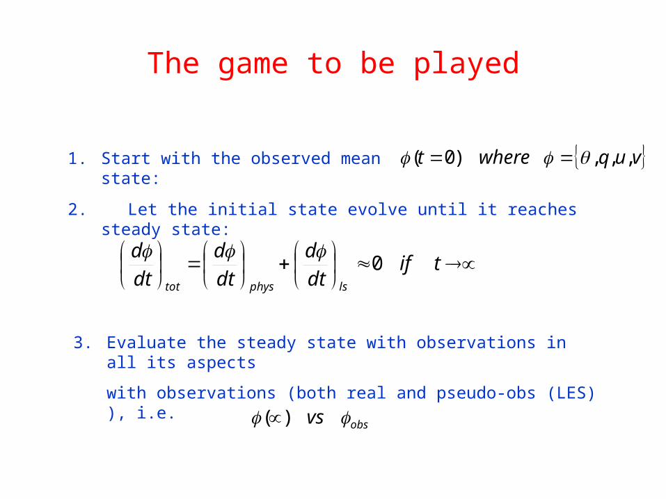
The game to be played

tifdt

d

dt

d

dt

d

lsphystot

0

vuqwheret ,,,)0( 1. Start with the observed mean state:

2. Let the initial state evolve until it reaches steady state:

3. Evaluate the steady state with observations in all its aspects

with observations (both real and pseudo-obs (LES) ), i.e.

obsvs )(

Two Flavours of the game

T

timeLSphys

dtdt

d

dt

dT

0

)0()(

1. Use the mean LS-forcing of the suppressed period:

2. Use directly the the time-varying LS forcing for the whole suppressed period.

i.e. the composite case.

T

LSphys

dtdt

d

dt

dT

0

)0()(

Model Type Participant Institute

CAM3/GB GCM (Climate) C-L Lappen CSU (US)

UKMO GCM (NWP/Climate) B. Devendish UK Metoffice (UK)

JMA GCM (NWP/Climate) H. Kitagawa JMA (Japan)

HIRLAM/RACMO LAM (NWP/Climate) W. De Rooy KNMI (Netherlands)

GFDL GCM (Climate) C. Golaz GFDL (US)

RACMO/TKE LAM (Climate S. De Roode KNMI (Netherlands)

COSMO NWP/regional/mesoscale J. Helmert DWD (Germany)

LMD GCM Climate) Levefbre LMD (France)

LaRC/UCLA LAM (Mesoscale) Anning Cheng NASA-LaRC (US)

ADHOC C-L Lappen CSU (US)

AROME LAM (Mesoscale) S. Malardel Meteo-France (France)

ECHAM GCM (Climate) R. Posselt ETH (Switzerland)

ARPEGE GCM (Climate) P. Marquet Meteo-France (France

ECMWF GCM (NWP) R. Neggers ECMWF (UK

Model PBL Scheme Convection Cloud

CAM3/GB TKE (bretherton/grenier) MF (Hack) Prog l,

UKMOK-profile/expl entr. /moist(?)

MF (Gregory-Rowntree)Mb=0.03w*

Stat/RH_cr (Smith)

JMAK-profile/expl entr/moist.

MF (Arakawa-Schubert) Stat/RH_cr (Smith)

HIRLAM/RACMO

TKE/moist MF(Tiedtke89)New entr/detr, M=a w* closure

Stat, diagns from K and MF

GFDLK-profile/expl entr/moist(?)

MF (Rasch) l,c prognostic

RACMO/TKE TKE moist MF (Tiedtke(89) l,c,prognostic

LMD Ri-number MF (Emanuel) Stat

LaRC/UCLA3rd order pdf basedLarson/Golaz (2005)

3rd order pdf basedLarson/Golaz (2005)

3rd order pdf basedLarson/Golaz (2005)

ADHOCAssumed pdfhigh order MF

Assumed pdfhigh order MF

Assumed pdfhigh order MF

AROME TKE-moist MF (pbl/cu-updraft) Stat. diagnostic

ECHAMTKE-moist Tiedtke(89) Entr/detr

(Nordeng)Stat Tompkins 2002)

ARPEGETKE-moist

MFStat ,cloud coverL=prognostic

ECMWF K-profile (moist) MF (pbl/cu-updraft) Stat. diagnostic

Submitted versions

Each model asked to submit:

• Operational resolution / prescribed resolution

• Operational physics / Modified physics

• Composite constant forcing / variable forcing

Initial State (identical to LES case)

Profiles after 24 hrs

Composite Case (High resolution)

80 levels ~ 100m resolution in cloud layer

Different Building Blocks

Moist Convection

entr/detr

M_b , w_u

Extended in bl

Cloud scheme:

stat

progn

Precip

precip?

microphysics

precip

PBL:K-profile

TKE

Higher order

ac, q

, q

acEstimating: ac,qlac,ql

on/off

• need increasingly more information from eachother

• demands more coherence between the schemes

At least in general much better than with the previous Shallow cumulus case based on ARM

(profiles after ~10 hours

Lenderink et al. QJRMS 128 (2002)

LES

Cloud fraction

In general too high

Time series

Composite Case (High resolution)

80 levels ~ 100m resolution in cloud layer

Some models behave remarkably well

• These models worked actively on shallow cumulus

• It seems that there are 3 crucial ingredients:

1. Good estimate of cloud base mass flux : M~ac w*

2. Good estimate of entrainment and detrainment

3. Good estimate of the variance of qt and l in the cloud layer in order to have a good estimate of cloud cover and liquid water.

Conclusions

• Mean state (slightly) better than for the ARM case

• Most models are unaccaptable noisy (mainly due to switching between different modes/schemes.

• Probably due to unwanted interactions between the various schemes

• No agreement on precipitation evaporation

• Performance amazingly poor for such a simple case for which we know what it takes to have realistic and stable response.

• Difficult to draw conclusions on the microphysics in view of the intermittant behaviour of the turbulent and convective fluxes.

We should clear up the obvious deficiencies

•Check LS Forcings: should we ask for it as required output?

• u,v –profiles : RACMO-TKE, ECMWF, UCLA-LaRC, ECHAM

•Ask for timeseries for u,v,q,T near surface to check surface fluxes and cloud base height off-line.

Required observational data

• Liquid water path (or even better profiles)

• cloud cover profiles (should be possible)

• .precipitation evaporation efficiency.

• Cloud base mass flux.

• Incloud properties., entrainment, detrainment mass flux (Hermann??)

• Variance of qt and theta (for cloud scheme purposes)

Further Points:

• Proceed with the long run??

•Get the the RICO-sondes into the ECMWF/NCEP analysis in order to get better forcings?

•Should we do 3d-GCM RICO?

Thank you

s

st qqtQ

Cloud cover

Bechtold and Cuijpers JAS 1995

Bechtold and Siebesma JAS 1999Wood (2002)

Statistical Cloud schemes

Convective and turbulent transport