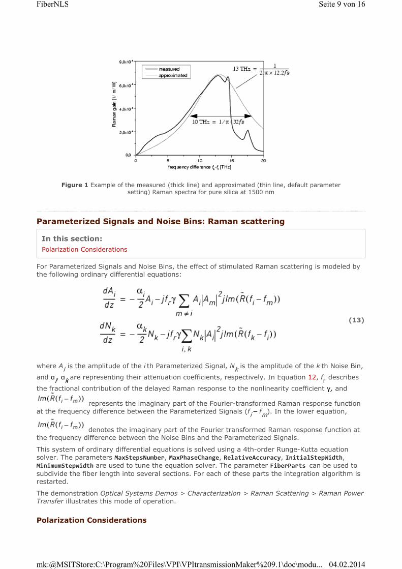
Photonic Modules > Fibers > FiberNLS FiberNLS Nonlinear Dispersive Fiber (NLS) Purpose When used with sampled-mode signals, this module solves the nonlinear Schroedinger (NLS) equation describing the propagation of linearly-polarized optical waves in fibers using the split-step Fourier method. Depending on the signal representation, different effects are represented: if the signals are in a Single Frequency Band (SFB), or JoinSampledBands = ON, the model takes into account stimulated Raman scattering (SRS), four-wave mixing (FWM), self-phase modulation (SPM), cross-phase modulation (XPM), first order group-velocity dispersion (GVD), second order GVD and attenuation of the fiber. If the signals are in a Multiple Frequency Band (MFB), the above effects are calculated within each band. Use the module UniversalFiber (or UniversalFiberFwd) to include interactions between MFBs and also between MFBs and Parameterized Signals. For Parameterized Signals (CW representation) an ordinary differential equation system including Stimulated Raman Scattering (SRS) and frequency dependent attenuation is applied. For this to operate ConvertToParameterized must be set to ON. Keywords Fiber, Nonlinear, Split Step, Raman, XPM, FWM, SPM, GVD Inputs Outputs Parameters In this section: Physical Numerical\Split-Step Parameters Numerical\Raman Parameters Enhanced Port Purpose Signal/Data Type input Input optical signal Optical Blocks Port Purpose Signal/Data Type output Output optical signal Optical Blocks Seite 1 von 16 FiberNLS 04.02.2014 mk:@MSITStore:C:\Program%20Files\VPI\VPItransmissionMaker%209.1\doc\modu...
Transcript
Photonic Modules > Fibers > FiberNLS
FiberNLS
Nonlinear Dispersive Fiber (NLS)
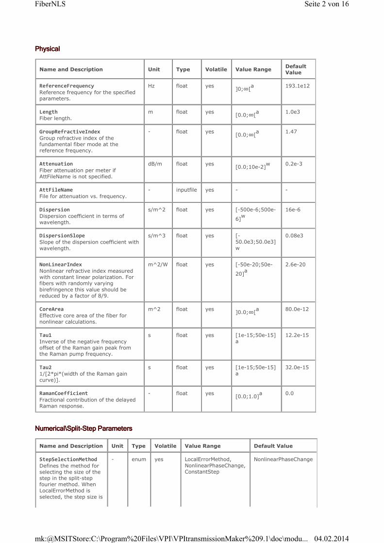
Purpose
When used with sampled-mode signals, this module solves the nonlinear Schroedinger (NLS)
equation describing the propagation of linearly-polarized optical waves in fibers using the split-step
Fourier method. Depending on the signal representation, different effects are represented: if the
signals are in a Single Frequency Band (SFB), or JoinSampledBands = ON, the model takes into
(SPM), cross-phase modulation (XPM), first order group-velocity dispersion (GVD), second order
GVD and attenuation of the fiber. If the signals are in a Multiple Frequency Band (MFB), the above effects are calculated within each band. Use the module UniversalFiber (or UniversalFiberFwd) to
include interactions between MFBs and also between MFBs and Parameterized Signals. For
Parameterized Signals (CW representation) an ordinary differential equation system including Stimulated Raman Scattering (SRS) and frequency dependent attenuation is applied. For this to
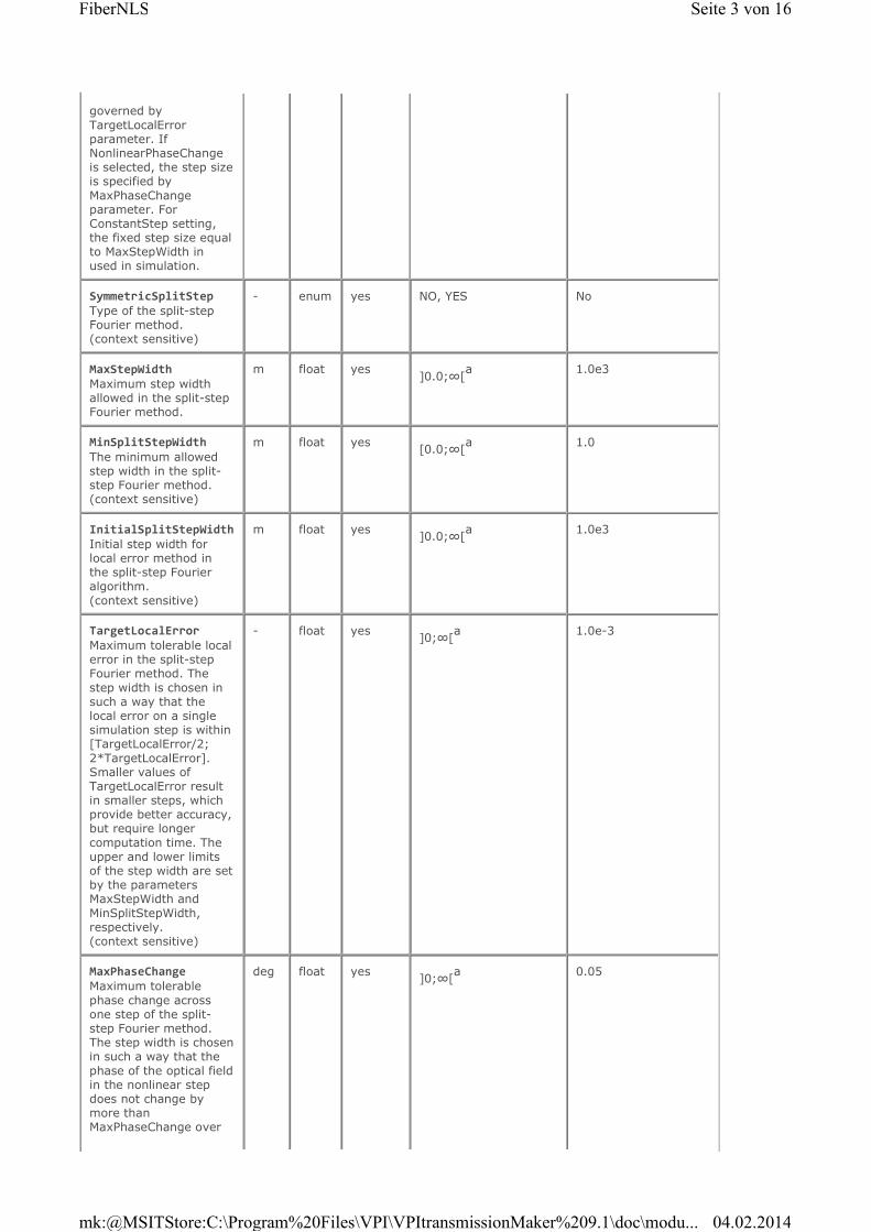
of MaxPhaseChange result in smaller steps, which provides better accuracy, but requires longer computation
time. The upper and lower limits of the step width is set by the parameters MaxStepWidth and MinSplitStepWidth,
respectively.(context sensitive)
Name and Description Unit Type VolatileValue
Range
Default
Value
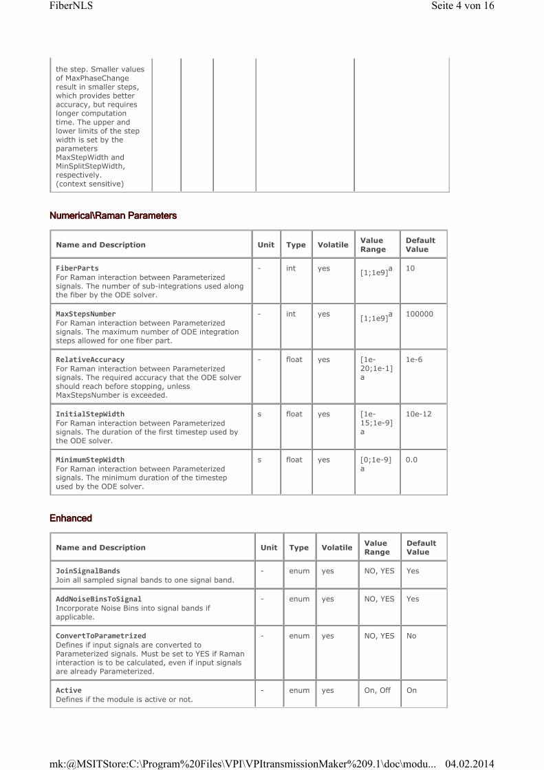
FiberParts
For Raman interaction between Parameterized signals. The number of sub-integrations used along the fiber by the ODE solver.
- int yes[1;1e9]
a 10
MaxStepsNumber
For Raman interaction between Parameterized signals. The maximum number of ODE integration steps allowed for one fiber part.
- int yes[1;1e9]
a 100000
RelativeAccuracy
For Raman interaction between Parameterized signals. The required accuracy that the ODE solvershould reach before stopping, unless MaxStepsNumber is exceeded.
- float yes [1e-
20;1e-1]a
1e-6
InitialStepWidth
For Raman interaction between Parameterized signals. The duration of the first timestep used by the ODE solver.
s float yes [1e-
15;1e-9]a
10e-12
MinimumStepWidth
For Raman interaction between Parameterized signals. The minimum duration of the timestep used by the ODE solver.
s float yes [0;1e-9]
a
0.0
Name and Description Unit Type VolatileValue Range
Default Value
JoinSignalBands
Join all sampled signal bands to one signal band.
- enum yes NO, YES Yes
AddNoiseBinsToSignal
Incorporate Noise Bins into signal bands if applicable.
- enum yes NO, YES Yes
ConvertToParametrized
Defines if input signals are converted to
Parameterized signals. Must be set to YES if Raman interaction is to be calculated, even if input signals are already Parameterized.
The sampled bands must contain a single signal polarization. However, unpolarized noise can be
propagated in Noise Bins. This is useful for saturating optical amplifiers with both polarizations of
noise. However, this unpolarized noise should not be added to the sampled band, as only a linear-
polarization sampled signal can be handled. This requires the Global Parameter InbandNoiseBins =
ON, and the fiber parameter AddNoiseBinsToSignal = OFF.
This is one of the simplest fiber models in the range. It is the basis of many fiber simulations. However, more complex fiber models are provided to offer more flexibility in terms of input data
format, interactions between signal representations, bidirectional Raman amplification, dispersion
decreasing fiber (UniversalFiber or UniversalFiberFwd), polarization mode dispersion
(FiberNLS_PMD), fast simulation of jitter in RZ systems (JitterLongHaul, JitterShortHaul), and
simulation with aperiodic waveforms (TimeDomainFiber).
Note: For simulations where the nonlinear effects are unimportant, simply set NonLinearIndex
to zero and ignore the parameters CoreArea, Tau1, Tau2, RamanCoefficient, and all settings in
the Numerical Parameters category.
The simulation speed of this module can be improved using parallel computations on a multi-core central processing unit (CPU) or a supported graphical processing unit (GPU), see Chapter 3, “User
Interface Reference” in the VPItransmissionMaker™/ VPIcomponentMaker™ User Interface Reference for details on supported hardware and GUI controls for parallel simulations.
The FiberNLS module can use parallel computations for the split-step Fourier algorithm. Both FFT
calculation and multiplication of the sample arrays will be done in parallel.
When both multithreading within modules and GPU-assisted computation are switched on and
supported by the hardware, the module will use the GPU, as it usually reduces the simulation time.
Note: Only calculations with sampled bands will be parallelized, both on the CPU and GPU.
Split-Step Fourier Implementation
In this section:
Dispersion OperatorNonlinear Operator (with no Raman effect)Split-Step Fourier Method
Nonlinear Operator (with Raman effect)
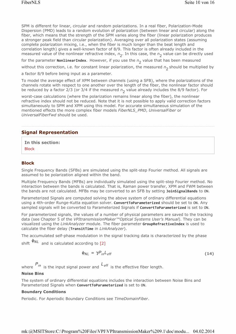
The generalized nonlinear Schrödinger equation is used to describe the inband effects:
where denotes the slowly-varying complex-envelope of the electric field of the light wave,
characterizes its power, is the nonlinearity operator, and is the dispersion
Note: For linear fibers, this is the only part of the theory that is required, as a single-section model will be applied if the NonLinearIndex is zero.
By removing changing the time reference to remove the intrinsic fiber delay, the dispersion
operator can be written as:
where:
The dispersion parameter, Dλ, has to be entered in SI units [10
-6 s/m
2= 1 ps/(km · nm)]
The dispersion slope parameter, Sλ, also has to be entered in SI units [10
3 s/m
3= 1 ps/
(km · nm2)]
Note: Setting the DispersionSlope to zero does not give a constant pulse spreading on each
WDM channel. This is because the dispersion is specified in terms of wavelength, but
implemented in terms of optical frequency. This is apparent when Dispersion and
DispersionSlope are set to zero, but there remains some pulse spreading.
The parameter AttFileName can be used to specify a file that contains the Attenuation
parameter [dB/m] vs. the optical frequency [Hz]. The file format is:193e12 0.2e3
193.1e12 0.2e3
193.2e12 0.2e3
Nonlinear Operator (with no Raman effect)
If stimulated Raman is to be excluded from the simulation (parameter RamanCoefficient = 0) the
nonlinear operator is simply given by:
(2)
β2 [s
2/m] describes the first order group-velocity dispersion (GVD), and is related to the
Dispersion parameter at the reference wavelength (= c/ReferenceFrequency) by
(3)
β3 [s
3/m] the second order GVD slope, and is related to the DispersionSlope S
λ= dD
λ/dλ by:
(4)
α [1/m] the attenuation constant. The Attenuation parameter a [dB/m] is related to α by
and depends on the nonlinear index n2 (parameter NonlinearIndex, see Polarization
Considerations), the effective CoreArea Aeff
, as well as on the reference frequency fref
and the
velocity of light in vacuum c.
Split-Step Fourier Method
The split-step Fourier method divides the fiber into alternate sections of two types. The first type
represents the dispersion in the frequency domain, the second represents the nonlinearity in the
time domain. The choice of step-size is crucial in achieving a balance between computation time
and accuracy.
The step size, Δz (the length of fiber represented by one nonlinearity and one dispersion operator)
is determined according to the following parameter settings:
When using the local error method, the following should be observed:
where Δφnl
(radians) is the maximum acceptable nonlinear phase shift1. The parameter
MaxPhaseChange sets the maximum acceptable phase change (but in degrees) and is normally
within the range of 0.06…0.2 degs.
Note: For both local error and nonlinear phase change methods, the step size is limited from
above and below by settings of the parameters MaxStepWidth and MinSplitStepWidth,
respectively.
If the desired step size is less than MinSplitStepWidth, the module will stop with an error
message. Normally, the minimal step size should be set as a ‘guard condition’ to ensure that the simulation will not take an excessive amount of time.
If the desired step size is larger than MaxStepWidth, the module will use the maximal allowed
step size. This is normally set to be far less than the walk-off length (the fiber distance that
produces a relative phase shift of 2π radians between the carriers) between two optical carriers due to dispersion. Obviously, the wider the WDM spectrum within a SFB, the shorter
the step length should be. This actually shows that it is better to model a few WDM channels
in an SFB, than all channels (this is called the Mean Field Approach, and is discussed in the VPItransmissionMaker™Optical Systems User’s Manual).
If StepSelectionMethod = LocalErrorMethod, the module takes the step according to the
algorithm described in [1], maintaining the relative error at each step within range [ε/2; ε],
where the desired error value ε is defined by the parameter TargetErrorValue. This mode is
rather similar to adaptive step algorithms routinely used in ordinary differential equations.
+ Local error method has greater order with respect to step size than the other optionsavailable for the fiber modules, which means that it will be more efficient (require less steps) for high-accuracy simulations. However, due to a larger number of computations per
step, low-accuracy simulations can be somewhat longer.
+ In some cases, such as propagation of several frequency components in a shifted-
dispersion fiber, local error method tends to make larger errors in low-power regions of the
spectrum (like the FWM products).
If StepSelectionMethod = NonlinearPhaseChange, the step size, Δzφ
, determined by not
allowing the nonlinear phase shift (proportional to optical power) to exceed a defined value,
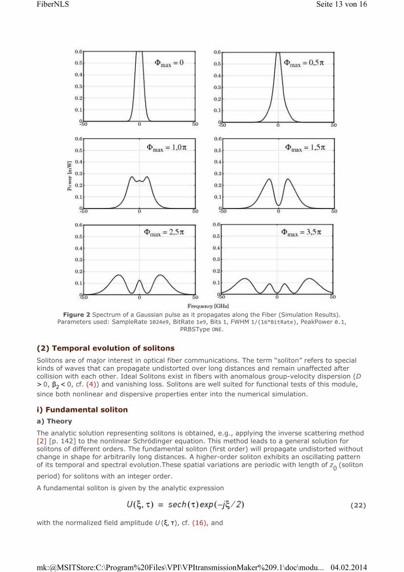
Figure 2 Spectrum of a Gaussian pulse as it propagates along the Fiber (Simulation Results). Parameters used: SampleRate 1024e9, BitRate 1e9, Bits 1, FWHM 1/(16*BitRate), PeakPower 0.1,
PRBSType ONE.
(2) Temporal evolution of solitons
Solitons are of major interest in optical fiber communications. The term “soliton” refers to special
kinds of waves that can propagate undistorted over long distances and remain unaffected after
collision with each other. Ideal Solitons exist in fibers with anomalous group-velocity dispersion (D
> 0, β2< 0, cf. (4)) and vanishing loss. Solitons are well suited for functional tests of this module,
since both nonlinear and dispersive properties enter into the numerical simulation.
i) Fundamental soliton
a) Theory
The analytic solution representing solitons is obtained, e.g., applying the inverse scattering method [2] [p. 142] to the nonlinear Schrödinger equation. This method leads to a general solution for
solitons of different orders. The fundamental soliton (first order) will propagate undistorted without
change in shape for arbitrarily long distances. A higher-order soliton exhibits an oscillating pattern of its temporal and spectral evolution.These spatial variations are periodic with length of z
0 (soliton
period) for solitons with an integer order.
A fundamental soliton is given by the analytic expression
with the normalized field amplitude U (ξ, τ), cf. (16), and
Therefore, for given values of γ and β2 and the pulse width T
FWHM, the peak power of a soliton of N
th order is uniquely defined.
b) Simulation
Propagation of first and second order solitons has been simulated using the setup which uses a
Pulse Sechant Transmitter, a Nonlinear Dispersive Fiber (NLS) module, and visualizers for the time and frequency domain. The first-order pulse should maintain its shape while propagating along the
fiber. This has been tested for up to 100 times the soliton period (approx. 10,000 km fiber length).
The results have been evaluated by comparing the data obtained with the analytical
expression (22).
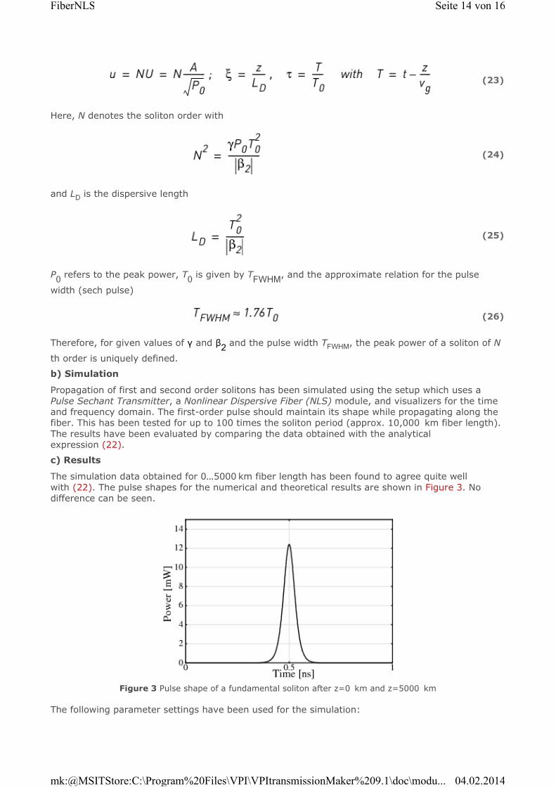
c) Results
The simulation data obtained for 0…5000 km fiber length has been found to agree quite well
with (22). The pulse shapes for the numerical and theoretical results are shown in Figure 3. No
difference can be seen.
Figure 3 Pulse shape of a fundamental soliton after z=0 km and z=5000 km
The following parameter settings have been used for the simulation:
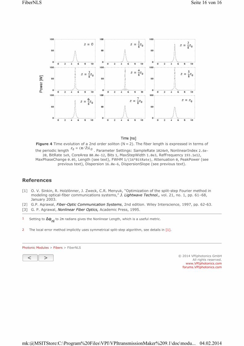
MaxPhaseChange 0.05, Length (see text), FWHM 1/(16*BitRate), Attenuation 0, PeakPower (see
previous text), Dispersion 16.0e6, DispersionSlope (see previous text).
References
Setting to Δφnl
to 2π radians gives the Nonlinear Length, which is a useful metric.
The local error method implicitly uses symmetrical split-step algorithm, see details in [1].
Photonic Modules > Fibers > FiberNLS
[1] O. V. Sinkin, R. Holzlönner, J. Zweck, C.R. Menyuk, “Optimization of the split-step Fourier method in modeling optical-fiber communications systems,” J. Lightwave Technol., vol. 21, no. 1, pp. 61–68,
January 2003.
[2] G.P. Agrawal, Fiber-Optic Communication Systems, 2nd edition. Wiley Interscience, 1997, pp. 62-63.
[3] G. P. Agrawal, Nonlinear Fiber Optics, Academic Press, 1995.