Sinusoidal Steady-state Analysis Complex number reviews Phasors and ordinary differential equations Complete response and sinusoidal steady-state

response Concepts of impedance and admittance Sinusoidal steady-state analysis of simple circuits Resonance circuit Power in sinusoidal steady –state Impedance and frequency normalization

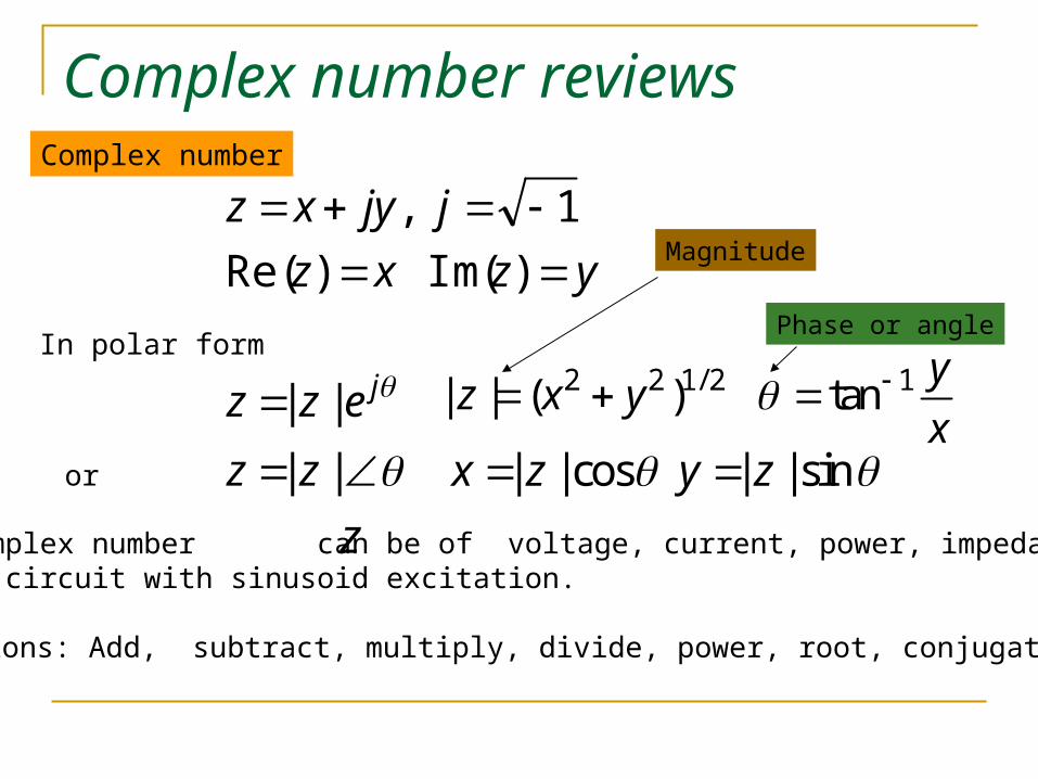
Complex number reviews

1, jjyxz

yzxz )Im()Re(

| | jz z e

Complex number

In polar form2 2 1/ 2 1| | ( ) tan

yz x y

x

| |z z or | | cos | | sinx z y z The complex number can be of voltage, current, power, impedance etc..in any circuit with sinusoid excitation.

z

Magnitude

Phase or angle

Operations: Add, subtract, multiply, divide, power, root, conjugate

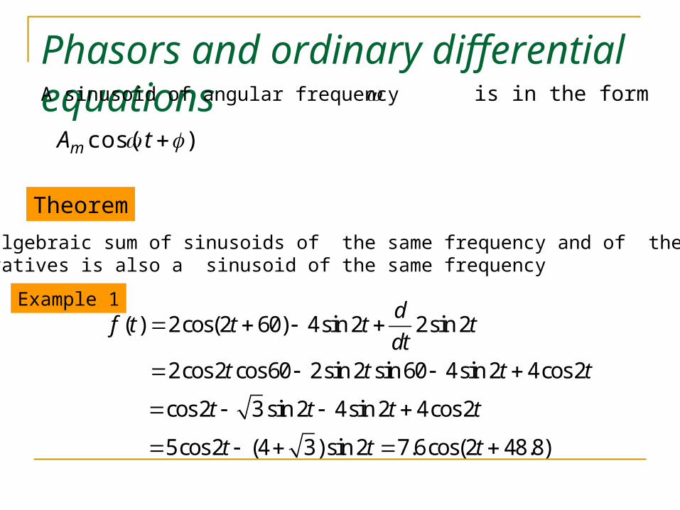
Phasors and ordinary differential equationsA sinusoid of angular frequency is in the form

)cos( tAm

Theorem

The algebraic sum of sinusoids of the same frequency and of their derivatives is also a sinusoid of the same frequency

Example 1

( ) 2cos(2 60) 4sin 2 2sin 2

2cos 2 cos60 2sin 2 sin 60 4sin 2 4cos 2

cos 2 3 sin 2 4sin 2 4cos 2

5cos 2 (4 3)sin 2 7.6cos(2 48.8)

df t t t t

dtt t t t

t t t t

t t t

Phasors and ordinary differential equations

jmA A e

)3/602cos(2110)( ttv

phasor form

Example 2

/ 3110 2 jA e (120 )( ) Re(110 2 )j tv t e

phasor

( )Re( ) Re( )

Re( cos( ) sin( ))

cos( ) ( )

j t j tm m

m m

m

A e A e

A t jA t

A t x t

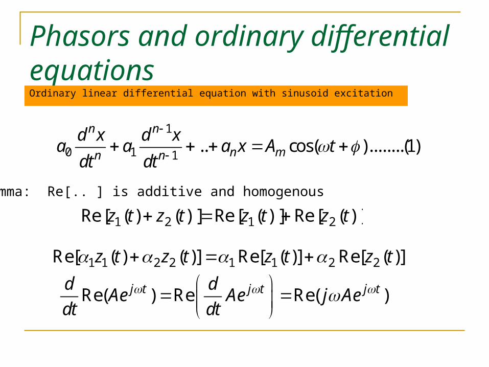
Phasors and ordinary differential equationsOrdinary linear differential equation with sinusoid excitation

1

0 1 1.. cos( )........(1)

n n

n mn n

d x d xa a a x A t

dt dt

Lemma: Re[.. ] is additive and homogenous

)](Re[)](Re[)]()(Re[ 2121 tztztztz

1 1 2 2 1 1 2 2Re[ ( ) ( )] Re[ ( )] Re[ ( )]z t z t z t z t

Re( ) Re Re( )j t j t j td dAe Ae j Ae

dt dt

Phasors and ordinary differential equationsApplication of the phasor to differential equation

,j jm mA A e X X e Let

substitute ( ) Re( )j tx t Xe in (1) yields

0 Re( ) .. Re( ) Re( )n

j t j t j tnn

dXe Xe Ae

dt

0Re( ) .. Re( ) Re( )n

j t j t j tnn

dXe Xe Ae

dt

0Re( ( ) ) .. Re( ) Re( )n j t j t j tnj Xe Xe Ae

Phasors and ordinary differential equations 10 1 1Re [ ( ) ( ) .. ( ) ] Re( )n n j t j t

n nj j j Xe Ae

12

10 1 1

10 1 1

2 2 3 22 1 3

[ ( ) ( ) .. ( ) ]

[ ( ) ( ) .. ( ) ]

[( .. ) ( ..) ]

n nn n

n nn n

mm

n n n n

j j j X A

AX

j j j

AX

even power odd power3

1 1 32

2

..tan

..n n

n n

Phasors and ordinary differential equations

)cos(||)Re()( tEEete tjs

Example 3

From the circuit in fig1 let the input be a sinusoidal voltage source and the output is the voltage across the capacitor.

+-

( ) | | cos( )se t E t

L R

C

+

-

( ) | | cos( )c cv t V t

( )se t( )cV t

i(t)

Fig1

Phasors and ordinary differential equations

)()()()( tetvtRitidt

dL sc

2

2

( ) ( )( ) ( )c c

c sd v t dv t

LC RC v t e tdtdt

)cos(||)Re()( tVeVtv ctj

cc

KVL

2[ )( ) ( ) 1] (2)cLC j RC j V E

Particular solution

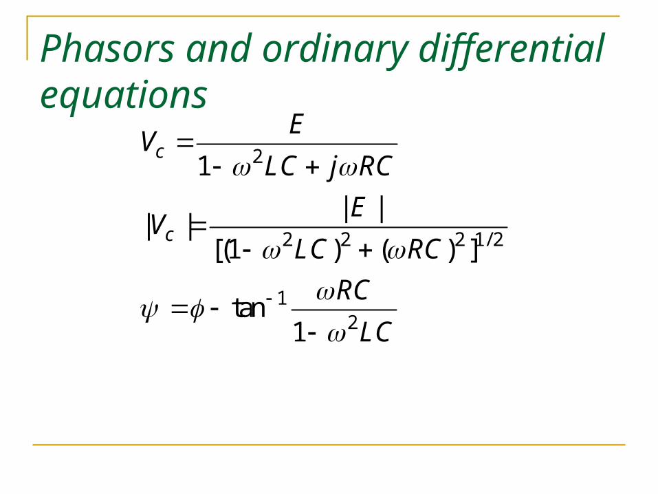
Phasors and ordinary differential equations

2

2 2 2 1/ 2

12

1

| || |

[(1 ) ( ) ]

tan1

c

c

EV

LC j RC

EV

LC RC

RC

LC

Complete response and sinusoidal steady-state responseComplete reponse

)()()( tytyty ph

)(ty p = sinusoid of the same input frequency (forced component)

( )hy t =solution of homogeneous equation (natural component)

1

( ) i

ns t

h ii

y t k e

(for distinct frequencies)

Complete response and sinusoidal steady-state responseExample 4

)(2cos)( tuttes For the circuit of fig 1, the sinusoid input is applied to the circuit at time . Determine the complete response of theCapacitor voltage. C=1Farad, L=1/2 Henry, R=3/2 ohms.

0t

1)0(,2)0( 0 cL vIi

2

2

( ) ( )1 3( ) cos 2 ( )

2 2c c

cd v t dv t

v t t u tdtdt

From example 3

Initial conditions

2)0()0(

,1)0(

C

i

dt

dvv Lcc

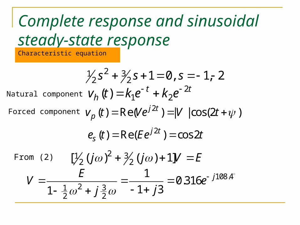
Complete response and sinusoidal steady-state responseCharacteristic equation

2,1,01232

21 sss

tth ekektv 2

21)( 2( ) Re( ) | | cos(2 )j t

pv t Ve V t

2( ) Re( ) cos 2j tse t Ee t

From (2) 2 312 2[ ( ) ( ) 1]j j V E

108.42 31

2 2

10.316

1 31jE

V ejj

Natural component

Forced component

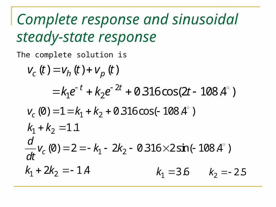
Complete response and sinusoidal steady-state responseThe complete solution is

21 2

( ) ( ) ( )

0.316cos(2 108.4 )

c h p

t t

v t v t v t

k e k e t

1 2

1 2

(0) 1 0.316cos( 108.4 )

1.1cv k k

k k

1 2

1 2

(0) 2 2 0.316 2sin( 108.4 )

2 1.4

cdv k k

dtk k

6.31 k 2 2.5k

Complete response and sinusoidal steady-state response

2( ) 3.6 2.5 0.316cos(2 108.4 )t tcv t e e t

The complete solution is

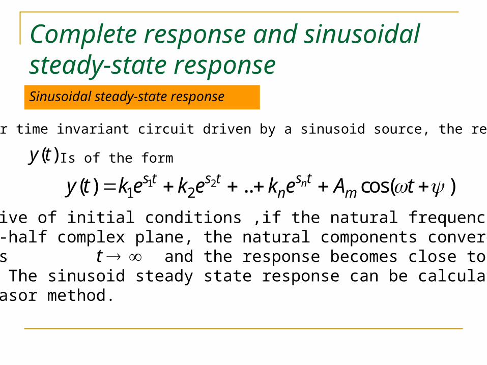
Complete response and sinusoidal steady-state responseSinusoidal steady-state response

)(ty

In a linear time invariant circuit driven by a sinusoid source, the response

Is of the form

1 21 2( ) .. cos( )ns ts t s t

n my t k e k e k e A t Irrespective of initial conditions ,if the natural frequencies lie in the left-half complex plane, the natural components convergeto zero as and the response becomes close to a sinusoid. The sinusoid steady state response can be calculated by the phasor method.

t

Complete response and sinusoidal steady-state response

40

220

4220

2 2)( sss

1 2 0 3 4 0,s s j s s j

0 01 2 3 4( ) ( ) ( )j t j t

hy t k k t e k k t e

Example 5

Let the characteristic polynomial of a differential a differential equationBe of the form

The characteristic roots are

and the solution is of the form

1 0 1 2 0 2( ) cos( ) cos( )hy t k t k t t In term of cosine

The solution becomes unstable as t

Complete response and sinusoidal steady-state response

0 01 2 0( ) cos( )j t j t

hy t k e k e K t

t0

220s

1 0 2 0,s j s j

( ) ( ) ( )h py t y t y t

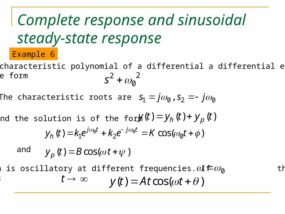
Example 6

Let the characteristic polynomial of a differential a differential equationBe of the form

The characteristic roots are

and the solution is of the form

( ) cos( )py t B t and

The solution is oscillatory at different frequencies. If the output is unstable as ( ) cos( )y t At t

Complete response and sinusoidal steady-state responseSuperposition in the steady state

If a linear time-invariant circuit is driven by two or more sinusoidalsources the output response is the sum of the output from each source.

Example 7

The circuit of fig1 is applied with two sinusoidal voltage sources and the output is the voltage across the capacitor.

+-

1 1 1cos( )mA t

L R

C

+

-

( )cV t

i(t)

+-

2 2 2cos( )mA t

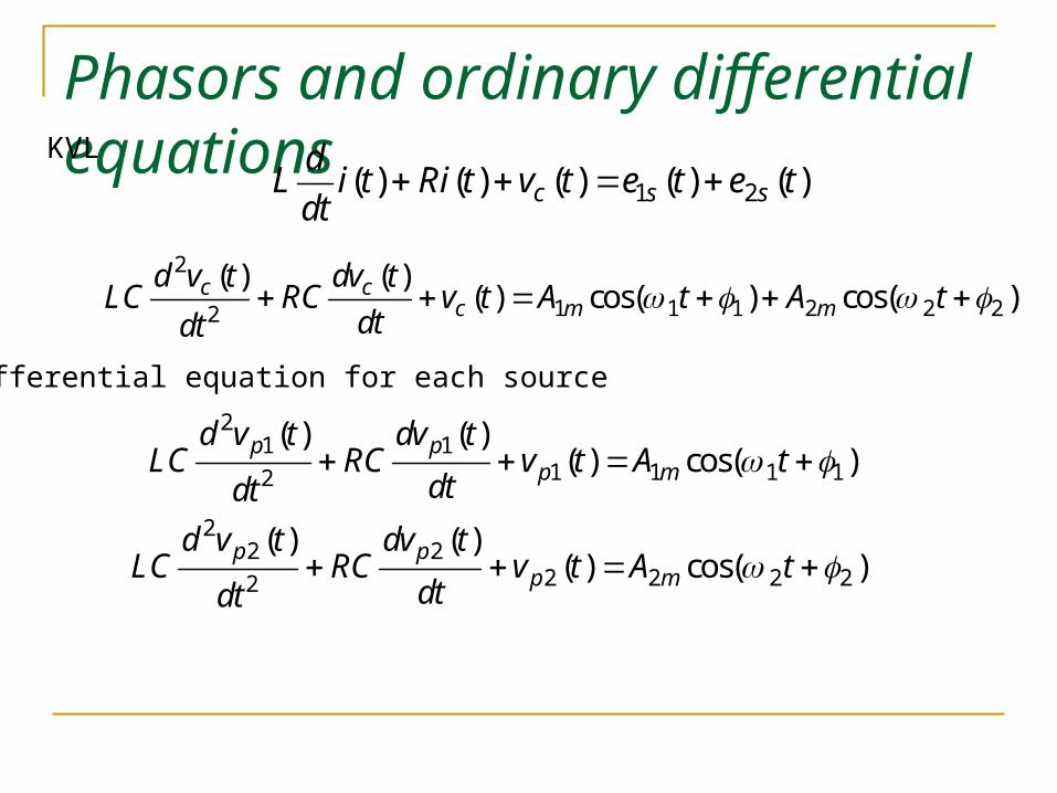
Phasors and ordinary differential equations

1 2( ) ( ) ( ) ( ) ( )c s sd

L i t Ri t v t e t e tdt

2

1 1 1 2 2 22

( ) ( )( ) cos( ) cos( )c c

c m md v t dv t

LC RC v t A t A tdtdt

21 1

1 1 1 12

( ) ( )( ) cos( )

p pp m

d v t dv tLC RC v t A t

dtdt

KVL

Differential equation for each source

22 2

2 2 2 22

( ) ( )( ) cos( )

p pp m

d v t dv tLC RC v t A t

dtdt

Phasors and ordinary differential equations

)cos()cos(

)()()(

22221111

21

tVtV

tvtvtv

mm

ppp

The particular solution is

11 1

22 2

( ) 11 2

1 1

( ) 22 2

2 2

1

1

jj m

m

jj m

m

A eV e

LC j RC

A eV e

LC j RC

where

Complete response and sinusoidal steady-state response

Summary

A linear time-invariant circuit whose natural frequencies are all withinthe open left-half of the complex frequency plane has a sinusoid steady state response when driven by a sinusoid input. If the circuit has Imaginary natural frequencies that are simple and if these are differentfrom the angular frequency of the input sinusoid, the steady-stateresponse also exists.

The sinusoidal steady state response has the same frequencyas the input and can be obtained most efficiently by the phasor method

Concepts of impedance and admittanceProperties of impedances and admittances play important roles in circuit analyses with sinusoid excitation.

Linear time-invariant circuit in sinusoid

steady stateElement

( ) Re( )j ti t Ie

( ) Re( )j tv t Ve

+

-

Phasor relation for circuit elements

( ) Re( ) | | cos( )j tv t Ve V t V

( ) Re( ) | | cos( )j ti t Ie I t I

Fig 2

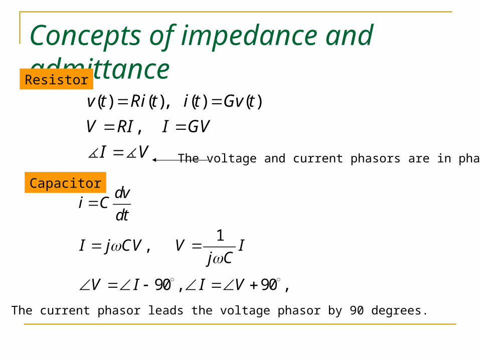
Concepts of impedance and admittance

( ) ( ), ( ) ( )

,

v t Ri t i t Gv t

V RI I GV

I V

Resistor

The voltage and current phasors are in phase.

Capacitor

1,

90 , 90 ,

dvi C

dt

I j CV V Ij C

V I I V

The current phasor leads the voltage phasor by 90 degrees.

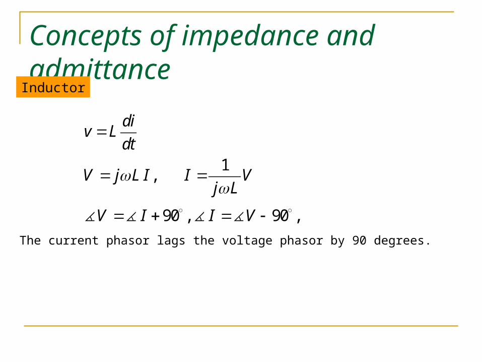
Concepts of impedance and admittanceInductor

1,

90 , 90 ,

div L

dt

V j L I I Vj L

V I I V

The current phasor lags the voltage phasor by 90 degrees.

Concepts of impedance and admittanceDefinition of impedance and admittance

The driving point impedance of the one port at the angular frequency is the ratio of the output voltage phasor V to the input current phasor I

| || ( ) | , ( )

| |

VZ j Z j V I

I

( ) | ( ) || | cos( )s sv t Z j I t Z I or

The driving point admittance of the one port at the angular frequency is the ratio of the output current phasor I to the input voltage phasor V

| || ( ) | , ( )

| |

IY j Y j I V

V

( ) | ( ) || | cos( )si t Y j V t Y V or

Concepts of impedance and admittance 1

| ( ) | , ( ) ( )| ( |

Z j Z j Y jY j

Angular frequency Z Y

Resistor

Capacitor

Inductor

RG

1

1

j Cj C

j L1

j L

R

Sinusoidal steady-state analysis of simple circuits

0)()()( 321 tvtvtv

0)cos()cos()cos( 332211 tVtVtV mmm

In the sinusoid steady state Kirchhoff’s equations can be written directlyin terms o voltage phasors and current phasors. For example:

If each voltage is sinusoid of the same frequency

1 2 3

1 2 3

1 2 3

1 2 3

Re( ) Re( ) Re( ) 0

Re( ) 0

Re[( ) ] 0

0

j t j t j t

j t j t j t

j t

V e V e V e

V e V e V e

V V V e

V V V

Sinusoidal steady-state analysis of simple circuits

n

n

VVVV

IIII

....

....

21

21

Series parallel connections

In a series sinusoid circuit

Z1 ZnZ2I

1I 2I nI1V+ - 2V - ++ nV -

+

-

V

1

( ) ( )n

ii

Z j Z j

Fig 3

Sinusoidal steady-state analysis of simple circuits

1 2

1 2

....

....n

n

V V V v

I I I I

In a parallel sinusoid circuit

Y1 YnY2

I

1I 2I nI

1V+

-2V

-

++nV

-

+

-

V

1

( ) ( )n

ii

Y j Y j

Fig 4

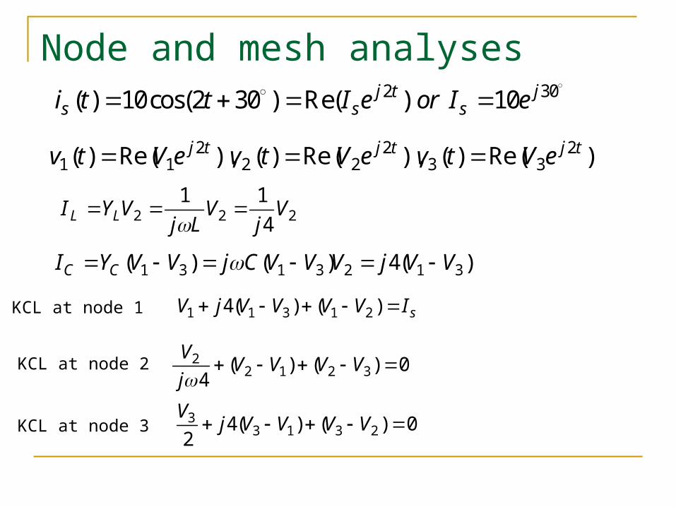
Sinusoidal steady-state analysis of simple circuitsNode and mesh analyses

)302cos(10)( ttis

Node and mesh analysis can be used in a linear time-invariant circuit todetermine the sinusoid steady state response. KCL, KVL and the conceptsof impedance and admittance are also important for the analyses.

Example 8

Fig 5

In figure 5 the input is a current source Determine the sinusoid steady-state voltage at node 3

1 32

2FCi

-

+++

--1v 2v 3v1W

1W 1W

2H 2W

Lisi

Node and mesh analyses2 30( ) 10cos(2 30 ) Re( ) 10j t j

s s si t t I e or I e

)Re()(),Re()(),Re()( 233

222

211

tjtjtj eVtveVtveVtv

1 1 3 1 24( ) ( ) sV j V V V V I

1 3 1 3 2 1 3( ) ( ) 4( )C CI Y V V j C V V V j V V

222 4

11V

jV

LjVYI LL

KCL at node 1

KCL at node 2 22 1 2 3( ) ( ) 0

4

VV V V V

j

KCL at node 3 33 1 3 24( ) ( ) 0

2

Vj V V V V

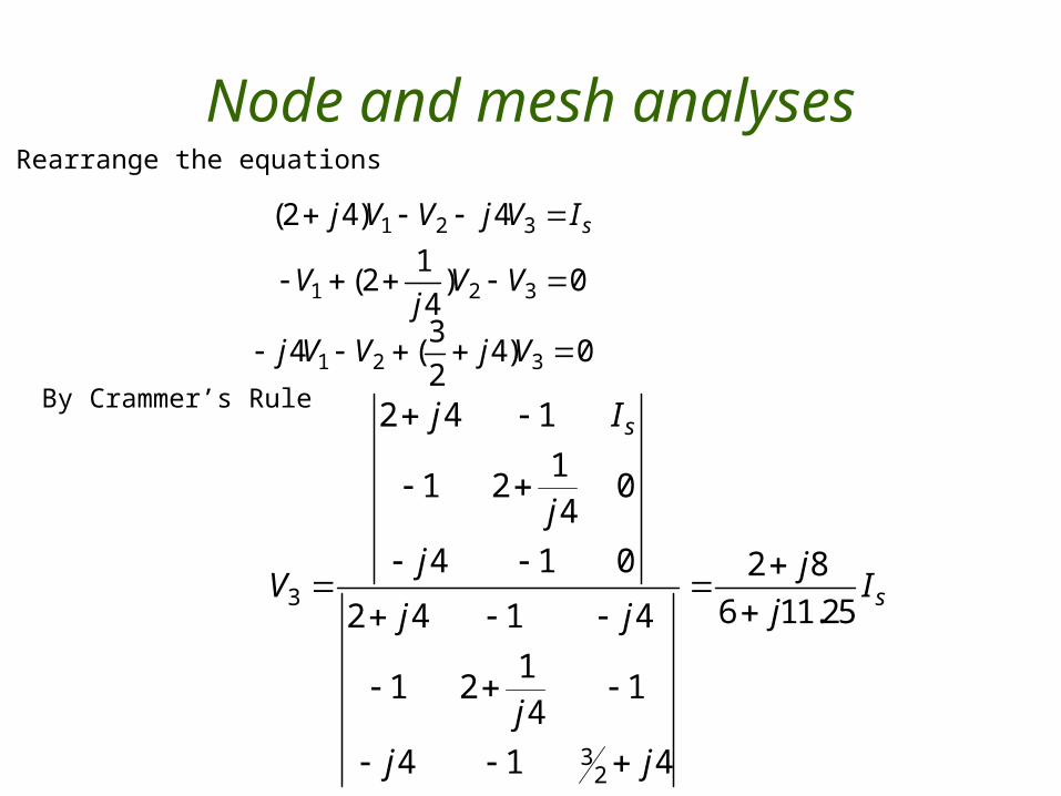
Node and mesh analysesRearrange the equations

1 2 3(2 4) 4 sj V V j V I

1 2 31

(2 ) 04

V V Vj

1 2 33

4 ( 4) 02

j V V j V By Crammer’s Rule

3

32

2 4 1

11 2 0

4

4 1 0 2 8

6 11.252 4 1 4

11 2 1

4

4 1 4

s

s

j I

j

j jV I

jj j

j

j j

Node and mesh analyses3010 j

sI e 44

3 6.45 jV e

3 ( ) 6.45cos(2 44 )v t t

Since

and the sinusoid steady-state voltage at node 3 is

Then

Example 9Solve example 8 using mesh analysis

2F

2i

-

++

-Lv 3v

1W

1W 1W

2H 2Wsv 1i 3i

+

-

Fig 6

Node and mesh analyses2 30( ) 10cos(2 30 ) Re( ) 10j t j

s s sv t t V e or V e

2 2 21 1 2 2 3 3( ) Re( ), ( ) Re( ), ( ) Re( )j t j t j ti t I e i t I e i t I e

1 1 2 1 3( ) 4( ) sI I I j I I V

3 31

C CV Z I Ij C

1 24( )L L L LV Z i j LI j I I

KVL at mesh 1

KVL at mesh 2

3 3 2 3 12 ( ) 4( ) 0I I I j I I KVL at mesh 3

2 2 3 3 11

( ) 4( ) 04I I I j I I

j

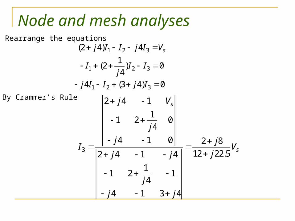
Node and mesh analyses

1 2 3(2 4) 4 sj I I j I V

1 2 31

(2 ) 04

I I Ij

1 2 34 (3 4) 0j I I j I By Crammer’s Rule

3

2 4 1

11 2 0

4

4 1 0 2 8

12 22.52 4 1 4

11 2 1

4

4 1 3 4

s

s

j V

j

j jI V

jj j

j

j j

Rearrange the equations

Node and mesh analyses

303 310 2j

sV e and V I

443 6.45 jV e

3 ( ) 6.45cos(2 44 )v t t

Since

and the sinusoid steady-state voltage at node 3 is

Then

The solution is exactly the same as from the node analysis

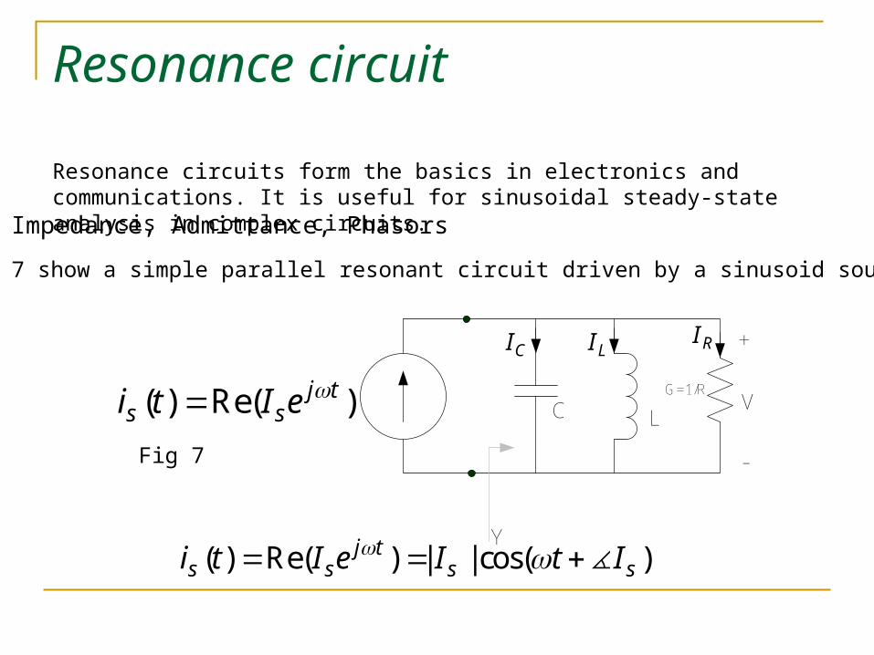
Resonance circuit

Resonance circuits form the basics in electronics and communications. It is useful for sinusoidal steady-state analysis in complex circuits.

( ) Re( )j ts si t I e C L

G=1/R

+

-

V

Y

CI LI RI

Impedance, Admittance, Phasors

Fig 7

Figure 7 show a simple parallel resonant circuit driven by a sinusoid source.

( ) Re( ) | | cos( )j ts s s si t I e I t I

Resonance circuit

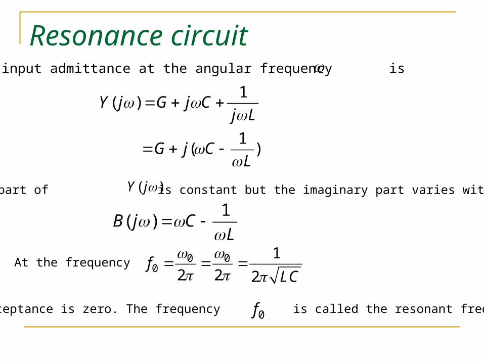
1( )

1( )

Y j G j Cj L

G j CL

( )Y j

The input admittance at the angular frequency is

The real part of is constant but the imaginary part varies with frequency

1( )B j C

L

At the frequency 0 00

1

2 2 2f

LC

the susceptance is zero. The frequency is called the resonant frequency.0f

Resonance circuit

LCjY

GjY

1

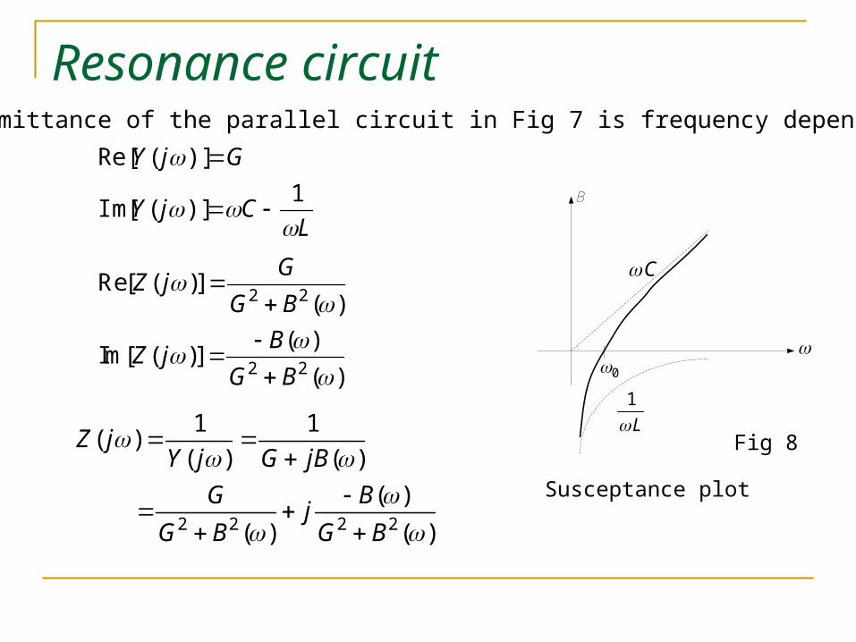
)](Im[

)](Re[

2 2

2 2

Re[ ( )]( )

( )Im[ ( )]

( )

GZ j

G B

BZ j

G B

2 2 2 2

1 1( )

( ) ( )

( )

( ) ( )

Z jY j G jB

G Bj

G B G B

The admittance of the parallel circuit in Fig 7 is frequency dependant

B

C

1

L

0

Susceptance plot

Fig 8

Resonance circuit

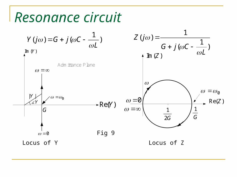
0

GRe( )Y

Im( )Y

| |YY

0

Admittance Plane

1( ) ( )Y j G j C

L

1( )

1( )

Z jG j C

L

Locus of Y

Re( )Z

0

Im( )Z

1

2G

1

G

0

Locus of Z

Fig 9

Resonance circuit

CVjIVLj

IGVI CLR

,1

,

SCLR IIII

)Re(cos)( jtss eItti

The currents in each element are

and

If for example1

1 , , 14

R L H C F W 0 , 1 /j

sI e rad s

The admittance of the circuit is

71.6( 1) 1 (1 4) 1 3 10 jY j j j e

The impedance of the circuit is71.61 1

( 1)( 1) 10

jZ j eY j

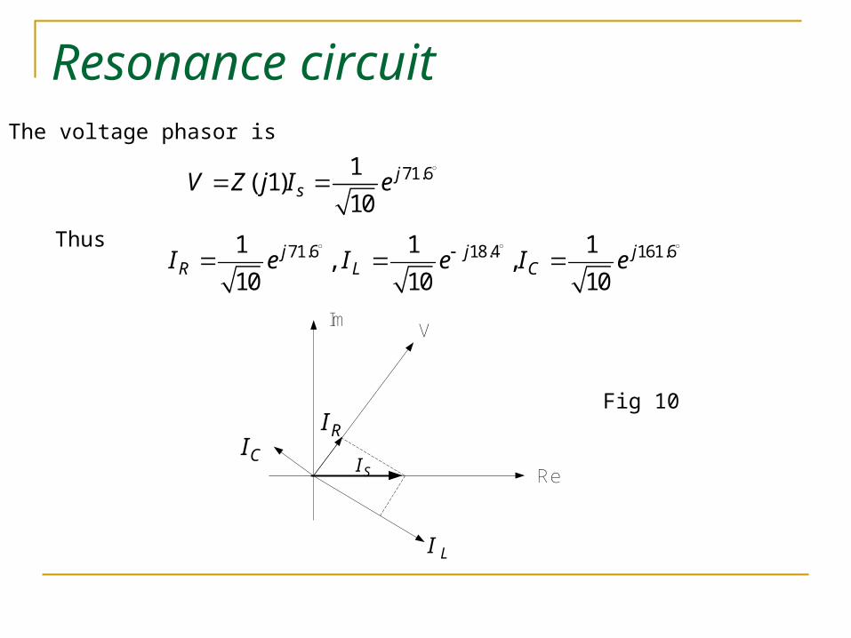
Resonance circuit

71.61( 1)

10j

sV Z j I e

71.6 18.4 161.61 1 1, ,

10 10 10j j j

R L CI e I e I e

The voltage phasor is

Thus

Re

ImV

LI

CIRI

SI

Fig 10

Resonance circuitsrad

LC/2

10 2( ) cos 2 Re( )j t

s si t t I e

0 , 2 /jsI e rad s

Similarly if and

( 2) 1, ( 2) 1, 1Y j Z j V 90 901, 2 , 2j j

R L CI I e I e

The voltage and current phasors are

Re

Im

V

LI

CI

R sI ISI

Note that it is a resonance and

,L s C sI I I I

Fig 11

Resonance circuit

| || |

| | | |pCL

ps s

RIIQ

I I L

1Q

)1

()(C

LjRjZ

The ratio of the current in the inductor or capacitor to the input current is the quality factor or Q-factor of the resonance circuit.

Generally and the voltages or currents in a resonance circuit is very large!

Analysis for a series R-L-C resonance is the very similar

( )( )s

sV

I jZ j

S R L CV V V V | || |

| | | |CL

ss s s

VV LQ

V V R

Power in sinusoidal steady-state

)()()( titvtp

The instantaneous power enter a one port circuit is

The energy delivered to the in the interval is

t

t

o

o

dttpttW ')'(),(

),( tto

Generator

( )i t

( )v t+

-

Fig 12

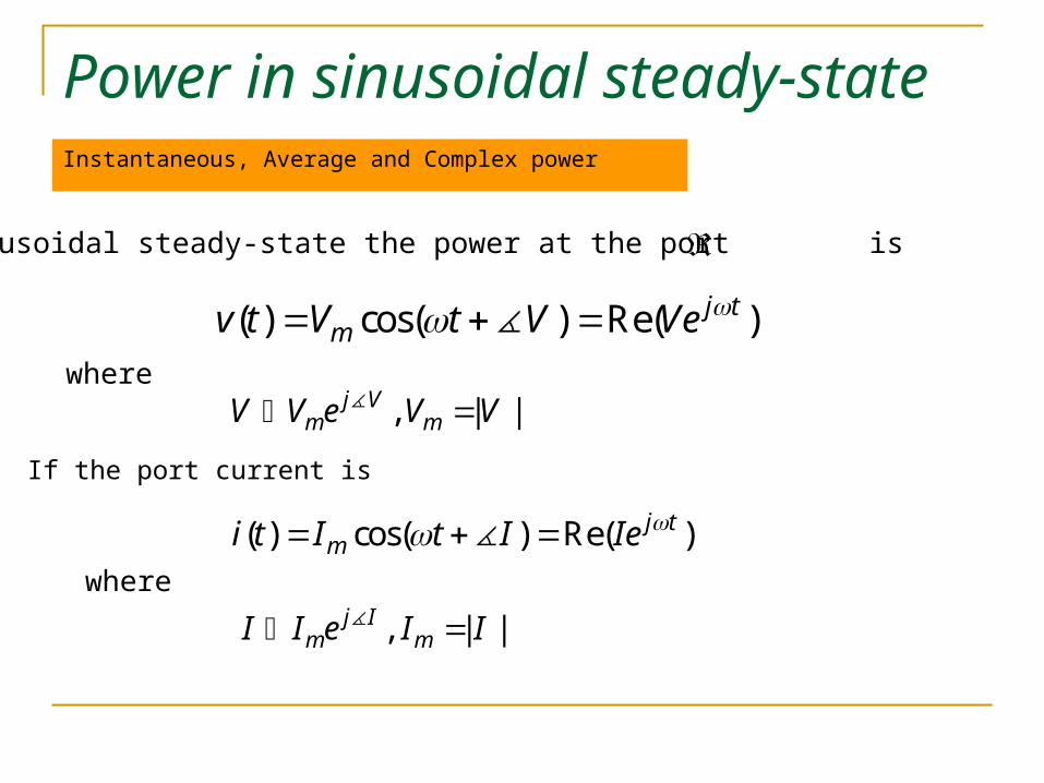
Power in sinusoidal steady-stateInstantaneous, Average and Complex power

In sinusoidal steady-state the power at the port is

( ) cos( ) Re( )j tmv t V t V Ve

, | |j Vm mV V e V V

where

If the port current is

( ) cos( ) Re( )j tmi t I t I Ie

, | |j Im mI I e I I

where

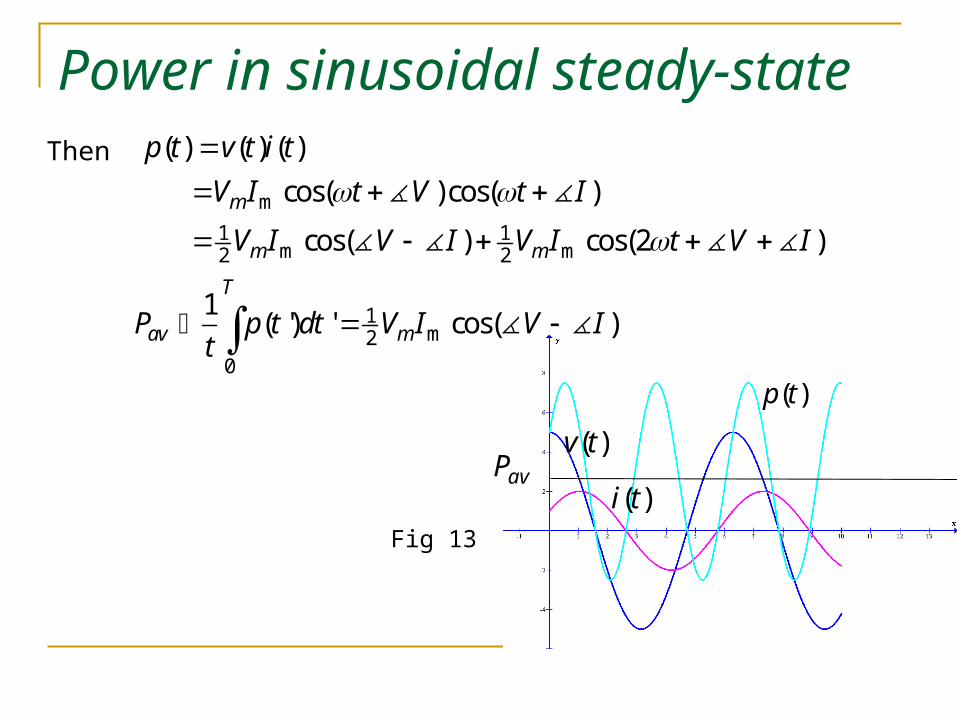
Power in sinusoidal steady-state

m

1 1m m2 2

( ) ( ) ( )

cos( )cos( )

cos( ) cos(2 )

m

m m

p t v t i t

V I t V t I

V I V I V I t V I

1m2

0

1( ') ' cos( )

T

av mP p t dt V I V It

)(tp

Then

avP)(tv

)(tiFig 13

Power in sinusoidal steady-state Remarks

The phase difference in power equation is the impedance angle

Pav is the average power over one period and is non negative. But p(t) may be negative at some t

The complex power in a two-port circuit is 12 rms rmsP V I V I

( )12

1 12 2

| || |

| || | cos( ) | || | sin( )

j V IP V I e

V I V I j V I V I

12

Re( ) Re( ) Re( )av rms rmsP P V I V I

2

2 21 12 2

2

| | Re[ ( )] | | Re[ ( )]

Re[ ( )] Re[ ( )]rms rms

avP I Z j V Y j

I Z j V Y j

Average power is additive

Power in sinusoidal steady-state Maximum power transfer

SL ZZ

The condition for maximum transfer for sinusoid steady-state is thatThe load impedance must be conjugately matched to the source imedance

s

sav R

VP

8

|| 2

max 2| |

4s

ss

VP

R

Q of a resonance circuit

00

212

0 212

| |

| |

RQ CR

L

C V

G V

For a parallel resonance circuit

0energy stored

Qaverage power dissipated in the resistor

(Valid for both series and parallel resonance circuits)

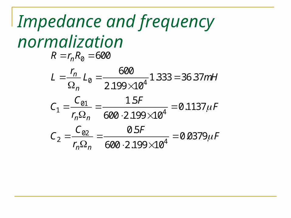
Impedance and frequency normalization In designing a resonance circuit to meet some specification component values are usually express in normalized form.

L

R

Qbandwidthdb

LCRZ 0

00 3,1

,

From

200

1,

RL C and

QR

Let the normalized component values are

0 0 01

1, ,R L Q CQ

Then0 0

0 20 0 0 0 0

1, ,

QZ ZR Z L C

Q Z Z

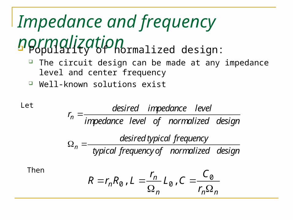
Impedance and frequency normalization Popularity of normalized design:

The circuit design can be made at any impedance level and center frequency

Well-known solutions exist

ndesired impedance level

rimpedance level of normalized design

Let

ndesired typical frequency

typical frequency of normalized designW

Then

nnn

nn r

CCL

rLRrR

W

W 0

00 ,,

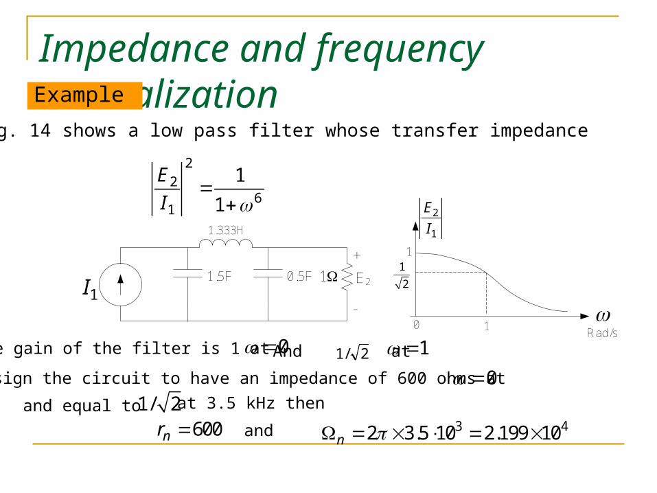
Impedance and frequency normalizationExample

6

2

1

2

1

1

I

E

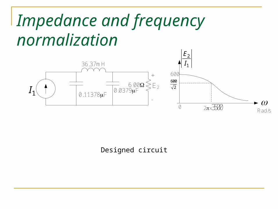
Fig. 14 shows a low pass filter whose transfer impedance

1I1.5F 0.5F

1.333H

1W+

-

E2

2

1

E

I

1

2

10Rad/s

1

The gain of the filter is 1 at 0 And at 1 Design the circuit to have an impedance of 600 ohms at 0 and equal to 1/ 2 at 3.5 kHz then

600nr 3 42 3.5 10 2.199 10n W and

2/1

Impedance and frequency normalization

0

0 4

011 4

022 4

600

6001.333 36.37

2.199 10

1.50.1137

600 2.199 10

0.50.0379

600 2.199 10

n

n

n

n n

n n

R r R

rL L mH

C FC F

r

C FC F

r

W

W

W

Impedance and frequency normalization

1I6 00W

+

-

E2

2

1

E

I

600

2

2x35000Rad/s

600

0.11378F0.0379F

36.37mH

Designed circuit