INDUSTRY STUDIES ASSOCATION WORKING PAPER SERIES Supermarket Characteristics and Operating Costs in Low-Income Areas By Robert P. King Food Industry Center University of Minnesota St. Paul, MN 55108 Ephraim Leibtag Economic Research Service United States Department of Agriculture (USDA) Washington, DC 20036 Ajay S. Behl Department of Applied Economics University of Minnesota St. Paul, MN 55108 2004 Industry Studies Association Working Papers WP-2004-12 http://isapapers.pitt.edu/
Transcript
INDUSTRY STUDIES ASSOCATION WORKING PAPER SERIES
Supermarket Characteristics and Operating Costs in Low-Income Areas
By
Robert P. King Food Industry Center
University of Minnesota St. Paul, MN 55108
Ephraim Leibtag
Economic Research Service United States Department of Agriculture (USDA)
Washington, DC 20036
Ajay S. Behl Department of Applied Economics
University of Minnesota St. Paul, MN 55108
2004 Industry Studies Association
Working Papers
WP-2004-12 http://isapapers.pitt.edu/
Supermarket Characteristics and Operating Costs in Low-Income Areas
Robert P. King, Ephraim Leibtag, and Ajay S. Behl
*
Abstract Research on low-income household food costs shows that the poor often have limited shopping opportunities and pay slightly higher prices for food. It is often hypothesized that higher prices are due, at least in part, to higher operating costs for stores that serve low-income households. This paper reports on research assessing how supermarket characteristics and operating costs differ with the percentage of sales derived from food stamp redemptions. Stores with a high percentage of revenues from food stamps generally offer fewer services that save time and add convenience for shoppers. They also offer a different mix of products, with a greater portion of sales coming from dry groceries and meat. Stores serving low-income shoppers use relatively little labor per 1,000 square feet of selling area. This helps keep labor costs as a percent of sales low, but gross margins for stores serving low-income consumers are also relatively low. Results from a cost function analysis indicate that stores serving low-income consumers are relatively well adapted to their market environment. But larger, more progressive supermarkets operated by major chains could provide significant competition for the typical store serving the urban poor. Overall, our results do not provide strong support for the hypothesis that it costs more to operate supermarkets that serve low-income consumers. *
Robert P. King is the E. Fred Koller Professor of Agricultural Management Information Systems in the Department of Applied Economics at the University of Minnesota. Ephraim Leibtag is an Economist in the Food Markets Branch, FRED-ERS-USDA. Ajay S. Behl is a Research Assistant in the Department of Applied Economics at the University of Minnesota. King and Behl are members of The Food Industry Center at the University of Minnesota. This research was funded by the Alfred P. Sloan Foundation through The Food Industry Center and by the Economics Research Service of the United States Department of Agriculture.
The findings presented here are still preliminary. Do not cite or quote this paper without permission from the authors.
Supermarket Characteristics and Operating Costs in Low-Income Areas
Do the poor pay more for food? This question has been the focus for a rich, sometimes
controversial stream of research over more than three decades. Findings have been mixed, often
due to differences in data, statistical methods, and the exact specification of the research question
(Kaufman et al.). Most of the evidence indicates that shopping opportunities for the poor are
more limited than they are for higher income consumers and that prices are slightly higher in
stores where low-income consumers do shop.
One often hypothesized reason for higher prices is that operating costs are higher for
stores that serve low-income households. The poor are more likely to shop in small grocery
stores that may have significantly higher operating costs than larger supermarkets. A study on
inner city grocery retailing by the Initiative for a Competitive Inner City (ICIC) noted that
supermarket operating costs may be higher in low-income areas due to higher occupancy costs,
less efficient store designs, higher rates of labor turnover, and/or greater losses due to theft.
Smaller average transaction sizes and procurement inefficiencies due to smaller orders to
suppliers may also increase costs. On the other hand, lower wage rates and tighter store designs
that use space more effectively help keep operating costs down in inner city stores that serve
low-income consumers (ICIC, pp. 10-11).
This study uses a unique data set – the Food Industry Center’s Supermarket Panel – to
assess how supermarket characteristics and operating costs differ in relation to the percentage of
sales derived from food stamp redemptions, an indicator of demand from low-income
consumers. Specific objectives for the study are:
1. compare and contrast store characteristics and operating practices of supermarkets in
low-income areas with those of higher-income areas,
2
2. compare and contrast operating costs for stores in low-income areas with those in higher-
income areas, and
3. empirically model and estimate the relationship between store characteristics and operating costs.
In the sections that follow, we first briefly describe data collection for the Supermarket Panel and
procedures used to merge the panel dataset with data from the U.S. Census and the STARS
database maintained by the Benefits Redemption Division of the U.S. Department of Agriculture
Food and Nutrition Food Stamp Program. Next, we present a descriptive analysis of Panel stores
grouped into quartiles based on the percentage of store sales derived from food stamp
redemptions. Because there are important differences in characteristics of stores located in urban
and rural areas, stores within each food stamp redemption quartile are also grouped by location
within or outside of an MSA. We then present an econometric analysis of store operating costs
for stores in the Supermarket Panel and use results from that analysis to investigate opportunities
for new store development in low-income areas. The final section of the paper summarizes
findings and conclusions from this study.
Data for the Study
The Supermarket Panel is an annual survey of supermarkets drawn at random from the
population of approximately 32,000 supermarkets that accept food stamps. In 2002, the study
year for this analysis, 866 stores participated in the Supermarket Panel. These stores – located in
forty-nine states – are generally representative of the diversity of formats and ownership
structures found in the overall population of U.S. supermarkets. Statistical weights adjust for
imbalances in sampling intensities and for differences in response rates by region and ownership
3
group size. In effect these weights indicate the number of stores in the overall population
represented by each store in the sample.1
Data from the 2002 Supermarket Panel were merged with zip-code specific data from the
U.S. Census, including data on population, spatial area, median household income, and the racial
composition of the population. In addition, store-level data on food stamp redemptions from the
STARS database maintained by the Benefits Redemption Division of the U.S. Department of
Agriculture Food and Nutrition Food Stamp Program were also merged with the Panel data set.
This made it possible to assess the degree to which each store serves low-income consumers.
A Descriptive Profile of Supermarkets Grouped by Food Stamp Redemption Rates
In this study the percentage of store sales attributable to food stamp redemptions serves
as a measure of the degree to which a store serves low-income shoppers. Average weekly store
sales data, as reported by participating store managers in early 2002, are part of the Supermarket
Panel database. Store level data on food stamp redemptions in 2001, the reference period for
respondents to the 2002 Supermarket Panel, were extracted from the STARS database and
divided by fifty-two to convert them to a weekly basis.
The percentage of sales from food stamp redemptions ranges from zero in about five
percent of stores to over thirty percent, with a weighted mean of 3.4 percent and a weighted
median of 2.1 percent. For this descriptive analysis, Panel stores are divided into quartiles based
on the percentage of sales from food stamp redemptions. Stores in Quartile 1 have the highest
food stamp redemption rates, while those in Quartile 4 have the lowest.
1 King, Jacobson, and Seltzer describe data collection for the 2002 Supermarket Panel in Appendix A of The 2002 Supermarket Panel Annual Report. A store’s ownership group size is the number of stores owned and operated by its parent company. Not all stores in an ownership group have the same name. For example, many of the largest food retailers own and operate stores under several distinct names.
4
Table 1 presents detailed information on store, market, and organizational characteristics
for stores grouped by food stamp redemption rates and location within or outside of an MSA.
Quartiles 2 and 3 for food stamp redemption rates have been combined. Differences between
MSA and non-MSA stores are relatively large for all of the characteristics included in this table.
With the exception of the median store age adjusted for recent remodeling and the percentage of
stores facing supercenter competition, all these differences are statistically significant.2
Cross-quartile differences in market characteristics are almost all statistically significant
for stores grouped by location. Median household income levels increase across quartiles for
stores located in and outside of an MSA, though the disparity between median household income
levels for stores in Quartiles 1 and 4 is much greater for stores located in an MSA. Similarly,
Differences in store characteristics are less pronounced and generally are not statistically
significant across quartiles for stores grouped by MSA or non-MSA location. It is noteworthy,
though, that Quartile 1 stores located in an MSA have a significantly lower median level of labor
intensity, measured by weekly labor hours per 1,000 square feet of selling area. For stores
located outside an MSA, the median level of labor intensity is not significantly different for
Quartile 1 and Quartile 2&3, though Quartile 4 stores do have a significantly higher level of
labor intensity. The difference in cross-quartile trends in the supply chain index for MSA and
non-MSA stores is also noteworthy. This index measures adoption of technologies and business
practices that support industry-wide initiatives to improver supply chain efficiency. Quartile 1
stores located in an MSA have the lowest average score, indicating that they are lagging in this
area. In contrast, Quartile 1 stores located outside of an MSA have a significantly higher average
score than stores in other quartiles.
2 Throughout this report we use a one-tailed significance level of 0.05 as the cutoff point for statistical significance. Details on statistical significance tests are available on request from the authors.
5
racial diversity is higher for stores in Quartile 1, but the percentage of nonwhite residents is
considerably higher for stores located in an MSA. In both MSA and non-MSA locations,
Quartile 1 stores are significantly more likely than Quartile 4 stores to face supercenter
competition. It is also noteworthy that the median distance to the nearest competitor is
significantly higher for Quartile 1 stores located in an MSA than for stores in other quartiles,
while the opposite it true for Quartile 1 stores located outside of an MSA. Quartile 1 stores
located in an MSA have a significantly lower median hourly wage, while cross-quartile
differences in median wage are not statistically significant for store located outside an MSA.
Finally, Quartile 1 stores located in an MSA are significantly more likely than stores in the other
quartiles to be wholesaler-supplied and they are significantly less likely to be owned by a
company with more than fifty stores. Cross-quartile differences in organizational characteristics
are much less pronounced for non-MSA stores. In each quartile, more than half of stores are
wholesaler-supplied, and ownership group size is more concentrated in the smaller categories.
Betancourt and Gautschi note that retail firms deliver a mix of explicit products and
services along with distribution services that reduce the time and effort customers need to devote
to shopping. For example, bagging and carryout are services that make checkout easier for
supermarket shoppers. Of course, offering a wider range of distribution services generally
increases store labor costs and prices charged for explicit products and services. Findings
reported by Kaufman et al. and Leibtag and Kaufman suggest that low-income shoppers adopt
economizing strategies to keep food costs as low as possible. Because low-income consumers
may be willing to sacrifice service and convenience for lower prices, stores serving them would
be expected to offer fewer distribution services. Similarly, the poor may also purchase a
different mix of food products and may be more likely to buy lower-cost private label products.
6
Table 2 presents information on service offerings and product mix. There are noteworthy
differences across quartiles and locations. Quartile 1 stores located in an MSA are generally
much less likely than other stores to offer distribution services that save time and add
convenience for shoppers. For example percentages of Quartile 1 stores that offer bagging and
carryout services are twenty percent below those for Quartile 2&3 stores. Post office/mailing
services and home delivery are exceptions to this pattern. Differences in service offerings are
much less pronounced and trends across quartiles are less consistent for stores located outside of
an MSA. In general, though, lower distribution service offering levels for Quartile 1 stores
suggest that, with a lower opportunity cost for their time and more stringent budget constraints,
the poor are willing to substitute their own time and effort for distribution services.
Percentages of store sales coming from produce, meat, and dry groceries exhibit similar
patterns across quartiles for stores located in and outside of an MSA. Quartile 1 stores that serve
low-income shoppers derive a greater share of sales from meat and dry groceries and a slightly
smaller share from produce. Quartile 1 stores located in an MSA are much less likely to have a
pharmacy with a full-time pharmacist. They also have a slightly greater share of sales from
private label products and offer less product variety, as indicated by the lower number of SKUs.
For non-MSA stores, there is no consistent pattern across quartiles in the percentage of stores
with a pharmacy or the share of sales from private label products, but Quartile 1 stores do have a
significantly higher median number of SKUs than stores in other quartiles.
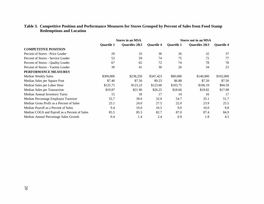
Table 3 presents information on competitive position and key performance measures for
stores grouped by food stamp redemption rates and location. The competitive position indicators
in the upper portion of the table are based on store managers’ identification of the price, service,
quality, and variety leader in their local market. For stores located in an MSA, Quartile 1 stores
7
are the least likely to be price and service leaders. This is consistent with findings from store-
level surveys of prices and with the data on distribution service offerings presented in Table 2.
Quartile 1 stores located outside of an MSA also are the least likely to be price leaders in their
local market, but they hold an intermediate position, relative to stores in other quartiles, in the
percentage of stores that are service and variety leaders.
Turning to the median performance measures in the lower portion of Table 3, there are
few significant differences across quartiles for sales per labor hour, sales per square foot, sales
per transaction, and inventory turns, regardless of location. There are no significant differences
between stores in Quartile 1 and those in Quartiles 2&3. On the other hand, the high median
employee turnover levels for Quartile 1 stores are a cause for concern, since high turnover can
significantly lower service quality and add to labor costs. Quartile 1 stores located in and outside
of an MSA have the lowest gross margins, though the difference is not significant for Quartile 1
and Quartile 2&3 stores located in an MSA. Lower margins may be due to higher cost of good
sold and/or lower prices charged to consumers. Quartile 1 stores also have significantly lower
payroll expenses as a percentage of sales. This is expected, since these stores offer fewer
distribution services, have less labor intensive operations, and pay lower wage rates. Median
cost of goods sold plus payroll as a percent of sales – a good measure of store operating costs
relative to sales – is lowest in both locations for stores in Quartile 4. This overall cost indicator
is essentially identical for typical stores in Quartile 1 and Quartiles 2&3 in both locations.
Finally, median annual sales growth for Quartile 1 stores in both locations is well below that for
other stores, and the typical Quartile 4 store enjoys a significantly higher growth rate.
To summarize, this descriptive analysis shows that stores serving low-income shoppers
differ in some important ways from other stores that receive less of their revenues from food
8
stamp redemptions. Stores with more revenues from food stamps generally offer fewer
distribution services that save time and add convenience for shoppers. These stores also offer a
different mix of products, with a greater portion of their sales coming from dry groceries and
meat and with greater reliance on sales of private label items. Despite paying lower hourly
wages than other stores, stores serving low-income shoppers use relatively little labor per 1,000
square feet of selling area. This helps keep labor costs as a percent of sales low, but gross
margins for stores serving low-income consumers are also relatively low. Overall, our results do
not provide strong evidence in support of the hypothesis that it costs more to operate
supermarkets that serve low-income consumers. Median cost of goods sold plus payroll as a
percentage of sales for stores with high food stamp redemption rates is not significantly different
from that for stores with moderate food stamp redemption rates.
Econometric Analysis of Store Operating Costs
The descriptive analysis in the preceding section focuses on differences in store
characteristics and operating costs associated with food stamp redemption rates and location
within or outside of an MSA. In this section we present a more comprehensive analysis of store
operating costs that controls for other store, market, and organizational characteristics.
The Supermarket Panel collects data on the two most important operating costs for most
supermarkets: cost of goods sold and payroll. Together these account for a major share of total
store operating costs, totaling 85.8% of sales for the median store in the Panel, and they will be
used as the sole measures of cost in this analysis.3
3 According to Food Marketing Institute (p. 13) estimates, the cost of sales plus all other operating expenses averaged 95.08% of sales for supermarket companies in 2000/2001. These costs were calculated at the company
Other operating costs are closely linked to
store selling area, which is treated as a quasi-fixed input in this analysis.
9
We model supermarket operating costs using a multiproduct translog specification with
productivity shifters, similar to that used by Fournier and Mitchell in their analysis of hospital
costs. This flexible form requires few assumptions about the production technology. It allows
for consideration of two outputs – store sales and retail services – and is well-suited for dealing
with some of the data limitations encountered in this study. Assuming a constant degree of
homogeneity for both outputs, the general form of the operating cost function for this analysis is:
Unit Price for Cost of Goods Sold (assumed to be $1)
SO Service Offerings Index SSize Store Selling Area TS Technology Shifter
With the assumption that PCOGS
level and include expenses for operation of distribution facilities and corporate offices. Building occupancy costs and energy costs are important store-level operating expenses for which data are not available. Both are sensitive to location and store size and format and can be viewed as quasi-fixed costs for any individual store. Results from an energy management study conducted in 2001 (King, Seltzer, and Poppert) indicate that energy costs are 1.1% of sales for the median store. Therefore, energy costs are small relative to cost of goods sold and payroll expenses.
is $1 for all stores, many of the terms in this general
specification fall out, since ln(1) = 0, but the parameters for these terms can generally be
10
recovered using the following parameter restrictions required to ensure that the cost function is
homogeneous of degree one in prices:
0,021
21,1
2
11TS,i
2
11SS,i
2
11SO,i
2
11WS,i2212121121 ∑∑∑∑
====
=γ=γ=γ=γ=γ+γ=γ+γ=α+α
Differentiation of the translog cost function with respect to ln(Wage) and ln(PCOGS
) and
application of Shephard’s Lemma yields two cost share equations, one for payroll and the other
for cost of goods sold. One of these is redundant because the two shares sum to one. The cost
share equation for payroll, LShare, retained in this analysis, is:
LShare Wage WSale SOSSize TS
WS SO
SS TS
= + + +
+ +
α γ γ γ
γ γ1 11 1 1
1 1
ln( ) ln( ) ln( )ln( ) ln( )
, ,
, ,
where TS once again represents a set of technology shifter variables.
Although the service offering level, SO, can be altered by store management, this output
variable generally reflects a longer run decision and so is assumed to be predetermined in our
statistical analysis. The level of weekly sales, WSale, is more problematic, however, because
this output variable is subject to random fluctuations that can affect both operating costs and the
payroll share of costs. In this analysis, we assume WSale is simultaneously determined with
operating costs and payroll share but not affected by them. Therefore, our model also includes
an equation for weekly sales:
)DSln()SSizeln()SOln()WSaleln( 3210 β+β+β+β=
where DS is a vector of exogenous demand shifter variables that includes some of the technology
shifter variables in the cost and payroll share equations. Assuming each of these three equations
has a normally distributed error term, we estimated this system of three equations using three-
stage least squares regression, imposing cross equation parameter restrictions where necessary.
11
The TS variable in the expressions above actually represents a set of factors hypothesized to
affect store operating costs. These include:
• binary variables for warehouse/supercenter format, WHSC, and a full-service pharmacy, Pharm, two store characteristics that, along with store selling area, are key indicators of store format;
• store age, adjusted for the most recent major remodeling, Age, a store characteristic that may affect operating efficiency;
• ownership group size, GSize, and a binary variable indicating whether the store and its distribution center are under common ownership, SDist, two important measures of store organization;
• an index relating the degree to which supply chain technologies and business practices have been adopted, SC;
• a binary variable indicating whether the store is located in an MSA, MSA; and • the percentage of sales attributed to food stamp redemptions, FS.
The annual labor turnover rate was also considered for inclusion in the model, since stores in low
income areas tend to have higher labor turnover and this has been hypothesized to drive up
operating costs. This measure was not available for many stores, however, which greatly
reduced overall sample size. Preliminary analysis indicated that estimates for parameters
associated with this measure were not jointly statistically significant at even the 0.40 level, so it
was excluded from the analysis.
The DS variable in the weekly sales equation represents a set of factors hypothesized to
affect the level of weekly sales. These include:
• population density, PopDen, and median household income, HHInc, for the store’s zip code, two important indicators of potential demand;
• binary variables indicating whether the manager believes his store is the local price leader, PrL, service leader, SerL, quality leader, QualL, or variety leader, VarL; and
• the following variables for the set of technology shifter variables: WHSC, Pharm, Age, GSize, MSA, and FS.
Parameter estimates for the operating cost, payroll cost share, and weekly sales equations
are presented in Tables 4, 5, and 6. The explanatory power for each of the three equations is
quite good for cross section data. Joint hypothesis tests were performed to determine the
12
statistical significance of each of the eight technology shifter variables in the model: WHSC,
Pharm, Age, GSize, SDist, SC, MSA, and FS. The parameters associated with each of these
variables are jointly significant at the 0.05 level.
Parameter estimates for the payroll cost share function are reported in Table 5. As
expected, the payroll cost share increases with increases in the wage rate. It also increases as the
level service offerings increases. This makes sense, since service offerings require labor but
have no cost of goods sold. On the other hand, the payroll cost share decreases as weekly sales
volume increases, indicating that there are significant savings in labor utilization per dollar of
sales as output increases along this dimension. Store selling area, which is treated as a quasi-
fixed input in this analysis, has no significant effect on the payroll cost share. Turning to the
eight technology shifter variables, the payroll share of cost is significantly higher in stores with a
full service pharmacy and in stores that are part of a self-distributing chain. It is significantly
lower for stores that belong to larger ownership groups, stores that have made more progress in
adopting supply chain technologies and practices, and stores with higher food stamp redemption
rates. The relatively strong effect for the food stamp redemption rate is consistent with findings
about the economizing behavior of low income shoppers who, with their lower opportunity cost
of time, are often willing to substitute their own labor for the labor of store employees that is
embodied in retail service offerings.
Signs of the parameter estimates for the weekly sales function reported in Table 6 are
also generally, though not always, consistent with expectations. Among market characteristics,
population density and median household income in the store’s location are positively related to
weekly sales, while location in an MSA and the food stamp redemption rate are negatively
related to weekly sales. Among store characteristics, ownership group size, store selling area,
13
warehouse or supercenter format, a full service pharmacy, and the number of hours open each
week are all positively related to weekly sales, while the level of service offerings and adjusted
store age are negatively related to sales. The negative relationship for service offerings runs
counter to expectations and may be due to problems with either model specification or the
definition of the service offerings variable. Finally, price, service, quality, or variety leadership
in the store’s local market area is associated with higher weekly sales, with price and quality
leadership having especially strong effects.
The large number of interactions in the full operating cost equation makes it difficult to
rely on direct inspection of parameter estimates to determine even the signs of marginal impacts
associated with changes in explanatory variables. To better understand these impacts, elasticities
for continuous explanatory variables and percentage change impacts for binary explanatory
variables were calculated for each food stamp redemption quartile, using the median values for
each explanatory variable that are presented in the upper portion of Table 7. Values of binary
variables that are the same for all quartile/location combinations are not shown. Elasticity and
percentage change estimates are presented in the lower portion of Table 7.
Stores that serve lower income consumers generally have lower payroll costs as a
percentage of sales. Therefore, it is not surprising that operating costs in these stores are
relatively insensitive to changes in wage rates in both MSA and non-MSA locations. The
elasticity of operating costs with respect to weekly sales is less than one for MSA stores in all
food stamp redemption rate groups, indicating economies of size with respect to this output
measure. This elasticity declines sharply across quartiles, indicating that size economies are
larger for stores with lower food stamp redemption rates. The elasticity of operating costs with
respect to weekly sales is greater than one for non-MSA stores in Quartiles 1 and 2&3, indicating
14
diseconomies of size. As expected, the operating cost elasticity with respect to the service
offerings index is positive for all store categories. Stores offering more distribution services
generally have lower cost of goods sold (and, therefore, higher margins) for the products they
sell, but these lower costs are more than offset by higher labor costs as a percent of sales. The
operating cost elasticity with respect to the store selling area is also negative for all store
categories, indicating that larger stores do enjoy important operational economies.
Turning attention to the technology shifter variables included in the model, elasticities
with respect to remodeling-adjusted store age and ownership group size are quite close to zero,
indicating that these store characteristics are not associated with important differences in
operating costs. Percentage cost savings associated with a shift to a warehouse or supercenter
format are relatively large for stores in all categories, while addition of a full service pharmacy
(none of the typical stores is assumed to have one) generally leads to slight increases in operating
costs. Operating cost elasticities with respect to the supply chain index are consistently negative,
which implies that there are significant cost savings at the store level associated with adoption of
these new technologies and business practices. Finally, operating cost elasticities with respect to
the food stamp redemption rate show no clear pattern across categories and are all relatively
small in absolute value. Once again, these results provide little, if any, support for the hypothesis
that stores serving low-income consumers have significantly higher costs.
Implications for New Store Development in Low-Income Areas
The ICIC study on inner city grocery retailing states that despite low incomes for many
residents, “… inner cities are the last large domestic frontier for retail, characterized by high
concentrations of income and limited competition.” (ICIC, p. 2). Attracting successful retail
15
operations can make low-income areas more vital and viable, not only by providing more
shopping opportunities in a more competitive environment but also by creating new employment
opportunities for area residents. The ICIC report goes on to present a series of case studies that
illustrate challenges in adapting retail store designs and business practices that are successful in
suburban markets for the inner city environment, noting that flexibility, patience, and a
willingness to experiment are critical.
Results from the cost function analysis conducted for this study can be used to investigate
whether stores with characteristics that are well-suited for moderate and high income market
settings can be competitive in lower income markets. Table 8 presents results of simulations in
which operating costs per dollar of sales were projected by combining store characteristics for
the typical store in each food stamp redemption quartile with typical market characteristics for
each quartile. The store characteristics include: service offerings, selling area, adjusted store
age, ownership group size, relationship with the primary supplier, supply chain index, and the
number of hours open each week. The market characteristics include: the wage rate, population
density, median household income, and the food stamp redemption rate. Values of these
variables for each quartile/location combination are given in the upper portion of Table 7.
The results for stores located in an MSA suggest that typical stores in each food stamp
redemption group are generally well adapted for their respective market settings. Values along
the diagonal from upper left to lower right of this portion of the table are operating cost
projections for the stores in their actual market settings. In each row (i.e., each market setting)
the value on this diagonal is either the minimum value or close to the minimum. In the Quartile
1 market setting, however, stores with characteristics typical of those in Quartiles 2&3 do have a
slight cost advantage. This suggests that the larger stores operated by major chains that also own
16
major distribution centers can be cost competitive in low-income urban areas. It is also
interesting to note that operating costs per dollar of sales for typical stores in each quartile
increase as market setting characteristics shift from those for Quartile 1 to those for Quartile 4.
This provides further support for the finding that supermarket operations in low-income urban
areas are not less cost efficient.
The results for non-MSA stores also indicate that typical stores for each quartile are well
adapted for their respective market settings. Once again, cost projections along the diagonal
from upper left to lower right of this portion of the table are at or near the minimum for their
respective rows. Characteristics of typical stores in Quartile 1 and in Quartiles 2&3 are quite
similar, as are projected operating costs per dollar of sales for these stores in low and moderate
income market settings. There is little evidence, then, that stores with characteristics of those
serving moderate and high income areas are likely to displace those currently operating in low-
income areas.
Summary and Policy Implications
This paper presents detailed descriptive information on store characteristics and operating
practices for supermarkets grouped by location and the percentage of sales derived from food
stamp redemptions. We find that stores serving low income consumers in MSA locations are
more likely to be wholesaler supplied and less likely to have adopted technologies and business
practices related to industry-wide supply chain initiatives. They are also located farther from
their nearest competitor than stores in higher income areas. However, operating costs as a
percentage of sales for stores serving low-income consumers are similar to those for stores with
moderate rates of food stamp redemption. In contrast, stores located outside of an MSA that
17
serve low income consumers tend to be slightly larger and more progressive than other non-MSA
stores in adopting supply chain technologies and practices, and they are located closer to their
nearest competitor. Once again, operating costs as a percentage of sales for stores serving low
income consumers are similar to those for stores with moderate rates of food stamp redemption.
Finally, regardless of location, stores serving low income consumers are less labor intensive and
offer fewer distribution services that make shopping more convenient and less time consuming.
Our econometric analysis of supermarket operating costs includes two output measures –
weekly sales and a service offerings index – and two variable inputs – labor and cost of goods
sold. Store selling area is treated as a quasi-fixed input. A number of store characteristics,
including the food stamp redemption rate, enter the model as cost shifters. Consistent with
findings from the descriptive analysis, increases in the food stamp redemption rate are associated
with a lower payroll cost share. After controlling for other factors, the food stamp redemption
rate has a relatively small, sometimes positive and sometimes negative effect on overall
operating costs. Operating cost projections for stores with characteristics typical of each food
stamp redemption quartile over a range of market settings indicate that store characteristics are
remarkably well adapted for their respective market settings. However, there do appear to be
opportunities for stores typical of moderate-income urban areas to move into low-income urban
areas.
Does it cost more to offer food retailing services to low-income consumers? Overall, our
results do not provide strong evidence in support of the hypothesis that it costs more to operate
supermarkets that serve low-income consumers. If the poor do pay more, factors other than
operating costs are likely to be the reason.
18
Table 1. Store, Market, and Organizational Characteristics for Stores Grouped by Percent of Sales from Food Stamp Redemptions and Location
Stores in an MSA Stores not in an MSA Quartile 1 Quartiles 2&3 Quartile 4 Quartile 1 Quartiles 2&3 Quartile 4 NUMBER OF STORES REPRESENTED 3,868 7,673 5,575 2,695 5,228 768 STORE CHARACTERISTICS Median Selling Area (sq. ft.) 29,000 35,000 32,000 22,000 21,000 13,000 Median Store Age (years) 25 18 22 23 24 30 Median Remodeling-Adjusted Store Age (years) 8 6 5 8 6 5 Median Hours Open per Week 112 119 112 102 112 100 Median Number of Checkout Lanes 8 9 10 6 7 5 Median Number of Parking Spaces 200 300 260 150 150 120 Median Labor Hours per 1,000 Square Feet 55.0 68.3 84.3 63.3 62.1 85.0 MARKET CHARACTERISITICS Median Population Density (people/sq. mi) 975 848 1563 68 74 75 Median Household Income ($/year) $42,654 $48,894 $61,182 $34,547 $38,242 $43,562 Percent of Sales from Food Stamps 7.4 1.8 0.3 6.8 2.3 0.3 Percent of Population - White 66.4 86.7 84.9 80.7 93.9 96.3 Percent of Population - Black 8.7 3.7 2.1 6.1 0.4 0.3 Percent of Population - Hispanic 4.5 2.8 3.4 2.6 1.6 1.2 Median Distance to Nearest Competitor (miles) 1.6 1.0 1.0 1.0 2.0 4.0 Percent Facing Supercenter Competition 53.0 53.6 32.4 59.7 44.4 23.0 Percent of Stores with Union Workforce 37.6 36.8 39.1 16.9 17.7 1.9 Median Hourly Wage $10.05 $11.52 $12.97 $9.20 $10.41 $9.89 ORGANIZATIOPNAL CHARACTERISITCS Median Ownership Group Size (# of stores) 22 180 65 22 15 1 Percent Wholesaler Supplied 55 34 50 65 53 66
19
Table 2. Service Offerings and Product Mix for Stores Grouped by Percent of Sales from Food Stamp Redemptions and Location
Stores in an MSA Stores not in an MSA Quartile 1 Quartiles 2&3 Quartile 4 Quartile 1 Quartiles 2&3 Quartile 4 DISTRIBUTION SERVICE OFFERINGS Percent Offering Self-Scanning 5 12 11 4 9 1 Percent Offering Bagging 70 91 94 90 98 99 Percent Offering Carryout 62 83 83 82 90 96 Percent Offering Service Meat 69 75 84 88 95 85 Percent Offering Fax Ordering 18 30 26 14 28 16 Percent Offering Home Delivery 16 11 21 12 31 19 Percent Offering Home Meal Replacement 45 66 80 61 65 66 Percent with In-Store Bakery 69 86 78 71 80 63 Percent Offering Internet Ordering 7 7 24 4 10 0 Percent Offering Post Office/Mailing Services 24 20 15 28 35 36 Percent with In-Store Banking 17 40 30 18 15 6 Percent with a Customer Web Site 60 72 73 60 52 22 PRODUCT MIX Median Percentage of Sales from Produce 8 8 10 7 8 8 Median Percentage of Sales from Meat 18 13 11 17 15 14 Median Percentage of Sales from Dry Groceries 54 49 47 62 50 51 Percent of Stores Selling Gasoline 10 9 4 1 6 16 Percent of Stores with a Pharmacy 25 44 44 17 28 11 Median Percentage of Sales from Private Label 17 15 11 18 20 12 Median Number of SKUs 19,000 25,000 35,000 31,000 20,000 28,000
20
Table 3. Competitive Position and Performance Measures for Stores Grouped by Percent of Sales from Food Stamp Redemptions and Location
Stores in an MSA Stores not in an MSA Quartile 1 Quartiles 2&3 Quartile 4 Quartile 1 Quartiles 2&3 Quartile 4 COMPETITIVE POSITION Percent of Stores - Price Leader 29 33 30 26 32 37 Percent of Stores - Service Leader 53 59 74 75 72 77 Percent of Stores - Quality Leader 67 65 72 74 78 78 Percent of Stores - Variety Leader 39 41 30 26 34 23 PERFORMANCE MEASURES Median Weekly Sales $309,000 $238,250 $347,423 $80,000 $140,000 $102,000 Median Sales per Square Foot $7.40 $7.56 $9.23 $6.88 $7.20 $7.50 Median Sales per Labor Hour $125.71 $123.23 $123.60 $103.75 $106.19 $94.59 Median Sales per Transaction $19.87 $21.90 $26.25 $18.66 $19.82 $17.08 Median Annual Inventory Turns 15 18 17 14 16 17 Median Percentage Employee Turnover 55.7 39.6 32.0 54.7 35.1 51.7 Median Gross Profit as a Percent of Sales 23.1 24.0 27.5 22.0 23.9 25.5 Median Payroll as a Percent of Sales 9.4 10.0 10.5 9.0 10.0 9.8 Median COGS and Payroll as a Percent of Sales 85.5 85.5 82.7 87.0 87.4 84.9 Median Annual Percentage Sales Growth 0.4 1.4 2.4 0.9 1.8 4.5