SMALL-AREA ESTIMATION AT IDESCAT:CURRENT AND RELATED RESEARCH

Albert Satorra and Eva Ventura

December 2006

Contents

1 Foreword 2

2 IDESCAT and small-area estimation 2

3 Standard approaches to small-area estimation 7

3.1 Design-based methods . . . . . . . . . . . . . . . . . . . . . . . . . . . . 8

3.1.1 No auxiliary information . . . . . . . . . . . . . . . . . . . . . . . 9

3.1.2 Regression estimator . . . . . . . . . . . . . . . . . . . . . . . . . 10

3.2 Model-based approach: mixed-effects regression . . . . . . . . . . . . . . 11

4 Longford’s research on small-area estimation 13

5 Other recent papers on small-area estimation 17

6 Conclusions 18

7 References 20

1

1 Foreword

This document presents perspectives of the research in small-area estimation carried out

by the team IDESCAT-UPF, composed of staff of the Catalan Statistical Institute and

the Department of Economics and Business, Universitat Pompeu Fabra, Barcelona, since

the year 2000. The work accomplished by the team is reviewed, together with the current

research on small-area estimation by Longford (2004 – 2007), and two recent papers on

the subject published in Survey Methodology.

2 IDESCAT and small-area estimation

The IDESCAT-UPF team was assembled as a response to practical needs of the Statis-

tical Institute of Catalonia (Institut d’Estadıstica de Catalunya, IDESCAT) to develop

an Industrial Production Index (IPI) for the Catalan autonomous community. The

Spanish National Institute of Statistics (Instituto Espanol de Estadıstica, INE) pro-

duces a monthly national summary of IPI only for Spain as a whole, and no summaries

for the country’s regions. With no budget for conducting a Catalan monthly survey,

IDESCAT estimated IPI for Catalonia for every year using the Spanish IPI of 150 indus-

trial branches. These were weighted according to their relative importance in Catalonia.

This IPI, based on a synthetic estimator, was accepted very well by the analysts of the

Catalan economy.

The statisticians at IDESCAT performed an assessment of the new index prior to its

publishing. The Statistical Institute for the Basque Country (Instituto Vasco de Es-

tadıstica, EUSTAT) conducted its own regional survey and published a Basque IPI.

IDESCAT created a synthetic index for the Basque Country, using the methodology

applied for the Catalan index. This index was compared to the EUSTAT’s IPI and the

results suggested that the synthetic index proposed by IDESCAT was acceptable (see

Costa and Galter 1994). Supported by this conclusion, IDESCAT produced a synthetic

IPI for Catalonia. Later INE applied the same methodology to derive a separate IPI for

each of the seventeen Spanish autonomous communities.

The method used by IDESCAT was by no means standard in the Spanish official statis-

tics. The synthetic IPI was criticized by some even though it was recognized to work

well in Catalonia. Some studies (Clar, Ramon and Surinach, 2000) showed that the

synthetic IPI works well in regions that have important and diversified industry, such as

3

Catalonia. But it fails in other Spanish regions. This observation encouraged IDESCAT

to investigate the theoretical basis of its synthetic IPI and to frame it in the context of

small-area estimation.

There is a varied methodology on small-area estimation. The reader can consult Platek,

Rao, Sarndal and Singh (1987), Isaki (1990), Ghosh and Rao (1994), and Singh, Gambino

and Mantel (1994) to gain an overview. Some of the methods use auxiliary information

from related variables for the estimation of area-level quantities. Recent work in San-

tamarıa, Morales and Molina (2004) deals with small-area estimation with auxiliary

variables and complex sampling designs.

Methods for small-area estimation include direct, synthetic and some other indirect es-

timators. Direct estimators use only data from the small area being examined. Usually

they are unbiased, but they exhibit a high degree of variation. Indirect, composite and

model-based estimators are more precise since they use also observations from related

variables or neighbouring areas. Indirect estimators are derived using estimators that

relate to and are unbiased for the entire domain. Composite estimators are linear com-

binations of direct and indirect estimators.

Due to the nature of the problem initially investigated, the research programme on small-

area estimation carried out by the IDESCAT-UPF team focused on models that involve

no covariates (auxiliary variables). An estimator that uses some auxiliary information

from other variables is in general more efficient, but introduces a degree of subjectivity.

We believe that only covariate-free small-area estimators can be used at the present stage

of our official statistics framework.

Alternative estimators of labor force at the regional level

Costa, Satorra and Ventura (2002) analyzed a survey in which direct regional estimators

of the Spanish work force were evaluated. They studied a synthetic, a direct, and a com-

posite small-area estimator and concluded that the composite and synthetic estimators

are almost identical in Catalonia, because this region’s economy is a large part of the

whole Spanish economy. The bias of the synthetic estimator was found to be very small

for Catalonia.

4

Comparison of alternative small-area estimators

Costa, Satorra and Ventura (2003) applied Monte Carlo methods (with both an em-

pirical and a theoretical population) to compare the performance of several small-area

estimators: a direct, a synthetic, and several composite estimators. Three versions of

the composite estimators are defined depending on the way they combine the direct and

synthetic estimators. One of them uses theoretical weights (based on known bias and

variance). Two others use estimated weights assuming homogeneous or heterogeneous

biases and variances across the small areas. The study concluded that for the sam-

ple sizes used in official statistics the composite estimator based on the assumption of

heterogeneity of biases and variances is superior.

Composite estimators for both domain and total area estimation

In Costa, Satorra and Ventura (2004), several alternative small-area estimators are com-

pared for both the domain and overall population quantities. Several sampling designs

and specific populations are used in the study. The following sampling designs are con-

sidered:

a) proportional design, in which the sample size of each area is proportional to the area

population size;

b) uniform design, in which each area has the same sample size, regardless of its pop-

ulation size, and

c) mixed design, which combined designs a) and b) with a given weight.

Design a) is optimal for estimating the parameter of the large area; design b) is well

suited for accurate estimation of quantities associated with the small areas. By using

composite small-area estimators we can either reduce the sample size for a given precision

or improve the precision when the sample size is fixed.

Improving small-area estimation by combining surveys

Costa, Satorra and Ventura (2006), henceforth CSV06, investigate how to integrate

information from an auxiliary survey in small-area estimation. This problem arises when

one tries to reconcile national and regional data-production systems. Many surveys and

5

administrative registers are of interest to both the country and its regions. The country’s

official statistics bureau has a much longer-standing tradition and greater resources, and

is usually in charge of producing survey-based statistics with a country-wide scope.

However, the statistics produced at the country level are sometimes not satisfactory for

the region.

A regional statistics office could conduct a similar survey, duplicated and improved for

its purpose, but that would amount to wasting resources and would increase the burden

on respondents. Some subjects (companies, households, and the like) would receive

virtually identical survey questionnaires, so they are likely to develop an impression that

the national and regional statistical offices do not coordinate their activities. In addition

to inducing a negative attitude towards official statistics, duplication of the respondents’

costs might be unreasonable.

As an alternative, regional statistical offices may ask the National Statistics Institute

(INE) to modify its survey design to meet the regions’ needs: to expand the questionnaire

to cover issues of regional interest, or to increase the sample size to achieve sufficient

precision for the inferences of interest. These changes would not cause problems in

sporadically conducted surveys. An example is the Survey of Time Usage conducted

in Spain on a single occasion in 2004. INE agreed to increase the subsample size in

some regions after negotiating with the regional statistical offices. This option may not

be available in some ongoing (annual, or quarterly) INE surveys that do not meet the

regions’ needs due to problems related to reliability or territorial disaggregation. Reasons

of technical, legal, or professional nature make modifications of the design of the ongoing

surveys problematic. The national offices could not cope with the myriad of requests

of various kinds from the regional offices. CSV06 investigate an analytical solution to

these problems that is based on supplementing the country-wide survey with auxiliary

information available for some of the small areas of interest.

Exploiting auxiliary information is not a new idea in small-area estimation. The direct

estimator uses information or data only from the area and the variable of interest. Direct

estimators are usually unbiased, though they may have large variances. When the direct

estimator for a particular small area is not satisfactory, one may resort to an indirect

estimator. An indirect estimator uses information from the small area of interest as well

as from other areas and other variables, or even from other data sources (other surveys,

registers or censuses).

6

Indirect estimators are based on implicit or explicit models that incorporate the available

information. For example, information obtained in a survey can be combined with the

one collected in a census or an administrative register. Indirect estimators are usually

biased, although their variances are smaller than for the direct (unbiased) estimators,

and the trade-off of bias and variance is usually in their favour. The novelty of the

approach in CSV06 is the use of an auxiliary survey instead of census or administrative

records. The information from a country-wide survey, called the reference survey (RS),

is combined with the information from a complementary survey (CS) conducted by the

regional statistics office and tailored to the specific needs of the small area.

A CS is conducted in the region concerned, its part, or in a few regions of the country

and records variables that correlate with the variables in RS. We regard CS as a ‘light

survey’, since its data are in general faster and cheaper to collect than for RS. For

example, in the case of unemployment, a subject in CS identifies him- or herself as

unemployed by the response to a single question. In contrast, RS follows the guidelines

set forth by the International Labour Organization to classify the subject as unemployed

(actively searching for work, available to begin working immediately, and so forth),

employed and economically inactive. CS can also simplify the process of contacting

the subjects (persons, companies, households, and the like) by using telephone contact

systems (Computer Assisted Telephone Interviewing, CATI) or other automated survey

methods. So, CS provides results similar to those of RS at a much lower cost; however,

as CS records the values of a slightly different variable than RS, its results are biased.

This is the price for the less elaborate questionnaire, with looser wording.

The accuracy of small-area estimators can be increased by:

a) increasing the sample size in the area of interest;

b) borrowing strength from neighbouring areas (using indirect or composite estima-

tors);

c) borrowing strength from CS, especially when the variables recorded in RS and CS

are highly correlated.

These alternatives are explored with emphasis on the options b) and c). The performance

of the estimators and the contribution of the complementary information are assessed

by simulation. Related work on the use of CS has been conducted by Costa et al (2006),

who study the Survey of the Use of Information and Communication Technologies in

7

Catalan households; INE conducts a country-wide survey while IDESCAT is in charge

of CS.

3 Standard approaches to small-area estimation

Sample surveys are used to estimate not only quantities related to the population (the

domain) but also quantities for sub-domains. An estimator is said to be direct if it is

based solely on the subsample for the sub-domain concerned. A domain direct estimator

is based only on the domain-specific sample data. A sub-domain (area) is regarded as

small if its subsample in the survey is not large enough to support direct estimation with

adequate precision.

For a small area, one could use indirect estimators that borrow strength by using values

of the variable of interest, Y , from related areas and/or time periods to increase the

effective sample size. An implicit or explicit model is used to link the different areas

and/or time periods, often through a source of auxiliary information, such as a census

or an administrative register.

We distinguish between the traditional indirect estimators based on implicit models and

the indirect estimators based on explicit small-area models. Synthetic and composite

estimators are examples of indirect estimators. They are generally design-based, in that

their probability distribution is induced by the sampling design. Their design variances

are usually small relative to the design variances of direct estimators. However, they are

biased and this bias is pervasive; it would not be reduced if the overall sample size were

increased. If the implicit linking model is valid, or at least approximately so, then the

design bias is small and the MSE is smaller than the MSE of the direct estimator.

Model-based estimators are derived from a stochastic model that distinguishes the within-

and between-area sources of variation that are not accounted for by auxiliary variables.

Inferences from model-based estimators refer to the distribution implied by the assumed

model. Model selection and validation play a vital role here. The models can be classified

into two types:

• Aggregate- (or area-)level models that relate small-area data summaries to area-

specific covariates. The values of the area-level summaries are assumed to satisfy

a population model. In particular, there is no information about the variation

within the areas, unless a suitable area-level summary is defined specifically for

8

this purpose.

• Unit-level models that relate the values of the units on the study variable to unit-

level (and in some models also area-level) covariates. For outcomes that are not

normally distributed, generalized linear mixed models may be applied. A crit-

ical assumption is that sample values satisfy the assumed population model; in

particular, the model has to account for any sample selection bias.

3.1 Design-based methods

Design-based methods assume a target population of fixed values, that is, a frozen pop-

ulation. The only random variation present is due to the sampling scheme; a replication

of the survey would yield a different sample, but it would be drawn from the same pop-

ulation, with the same division of the domain to areas. Information is required about

population summaries (statistics), such as the mean, median or total of a variable and the

ratio of two means. In a small-area setting, the population is composed of sub-domains

(areas), and information is required about summaries at the area level.

First we introduce some notation. The target population U consists of N distinct el-

ements (elementary units) labeled j = 1, 2, . . . , N . We observe the characteristics of a

sample of units, yi , i = 1, . . . , n. We assume that there is no measurement error and the

sample is observed completely, without any values missing. The parameter of interest

is either the total Y + = (Y1 + Y2 + · · ·+ YN) or the average, Y = Y +/N . With an

indicator target variable, which attains only values of 1 (positive) and 0 (negative), the

total Y + corresponds to the count and mean to the proportion of positives. We assume

that we have an estimator Y + of the total Y +, based on all the elements of the sample s.

The sampling design is defined by the probability distribution p(s) according to which

a sample s is selected from U . This probability may depend on known design variables,

such as stratum indicators, size of the cluster, and the like.

The estimator is design-unbiased (or p-unbiased) if

Ep

(Y +

)=∑s⊂U

p(s)Y +(s) = Y + ,

where Y +(s) denotes the value of the statistic Y + for sample s and the summation is

over all subsamples of the population. The design variance of Y + is

Vp(Y ) = Ep

{Y − Ep

(Y)}2

,

9

and it is estimated by v(Y +

)= s2

(Y +

). This estimator is p-unbiased if

Ep

{v(Y +

)}= Vp

(Y +

).

The estimator Y + is p-consistent if both its bias and variance Vp

(Y +

)tend to zero

as the sample size increases. p-consistency of any other estimator is defined simi-

larly. Together with asymptotic normality, it implies that in repeated sampling, and

with samples of large size, about 100(1 − α)% of the (random) confidence intervals[Y + − zα/2 s

(Y +

), Y + + zα/2 s

(Y +

)]contain the (fixed) value of Y + ; zα/2 is the

(1− 1

2α)-

quantile of the standard normal distribution, N(0, 1). The design-based approach has

been criticized on the grounds that the associated inferences refer to repeated sampling

instead of conditioning on the particular sample that has been drawn.

3.1.1 No auxiliary information

For estimating the total for a variable observed in the survey there are several possibili-

ties.

Design-unbiased estimation with no auxiliary information

We can use the expansion estimator of Y + for the population U , defined as Y + =∑

j wjyj

where wj is the design-weight, and∑

j denotes the summation over the units of the

sample. Denote by ri the probability that unit i is included in the sample. That is,

ri =∑

s3i p(s). The expansion estimator is unbiased when wi = 1/pi .

Under stratified multistage sampling, the expansion estimator can be expressed as

Y =∑j

wh`k yh`k ,

where the subscripts indicate element k in the primary sampling unit (cluster) ` belonging

to stratum h. The summation is over all elements j = (h`k) of the sample. We treat

the sample as if the clusters were sampled with replacement and subsampling is done

independently for each selected cluster.

For estimating the total for a subpopulation Ui , we construct the variables

Yij =

{Yj if j ∈ Ui

0 otherwise

10

and

Aij =

{1 if j ∈ Ui

0 otherwise

Note that Yij = Aij Yi . We have

Y +(Yi) =∑j

Yij =∑j

Yi = Y +i

and

Y +(Ai) =∑j

Aij =∑j

1 = Ni .

The domain mean Y = Y +(Yi)/Y +(Ai) is estimated by

ˆY i =Y +(Yi)

Y +(Ai)=

Y +i

Ni

and ˆY i = Y +i /Ni if the subpopulation size Ni is known. If Yj is binary and takes the

values 0 or 1, then ˆY i = Pi , an estimator of the domain proportion Pi . If the expected

domain sample size is large, the ratio estimator ˆY is p-consistent. A Taylor linearization

variance estimator is given by

V ( ˆY i) =V (ei)

N2i

,

where ei = yij − ˆY i aij .

3.1.2 Regression estimator

Suppose auxiliary information is available in the form of known population totals X+ =(X+

1 , . . . , X+p

)>and the values of X are observed in the sample. The generalized regres-

sion (GREG) estimator is defined as:

Y +GR = Y + +

(X+ − X+

)>B ,

where Y + and X+ are the expansion estimators and B = (B1 , . . . , Bp)> is the solution

of the sample weighted least-squares equations:(∑s

wj

cj

xjx>j

)B =

∑s

wj

cj

xjy>j

with specified positive constants cj . When the first component of xj is set to unity and

cj = 1, we obtain the linear regression estimator

YLR = Y +(X − X

)>BLR .

11

The Taylor linearization method yields the approximation VL

(YLR

) .= V(e), where e

are the residuals of the regression fit. Several modifications of this formula have been

developed to deal with particular circumstances.

3.2 Model-based approach: mixed-effects regression

In the model-based approach, we assume that the data analyzed is a realization of a

stochastic process characterized by some parameters (mean, ratios, and the like), whose

values are the target of the analysis. Random variation arises here by the nature of the

data-generating process. The sub-domains of the population are a layer of random varia-

tion also characterized by specific parameters. In this approach, methods for small areas

estimate (predict) the domain-level realizations of the constituents of a (hierarchical)

random-coefficient model.

Small-area models may be regarded as special cases of a general linear mixed model

involving fixed and random effects (e.g., Prasad and Rao, 1990; Jiang and Lahiri, 2006).

Means or totals for the areas can be expressed as linear combinations of fixed and random

effects. Best linear unbiased predictors (BLUP) of such quantities can be obtained in

the classical frequentist framework by appealing to the general results in the theory of

BLUP. BLUPs minimize the MSE in the class of linear unbiased estimators and do not

require the assumption of normality of the random effects. In this section, we review this

general modeling approach as it applies to small-area estimation. An early application

of this approach is by Ericksen (1973) and (1974), who uses the terms criterion variable

and symptomatic information for the dependent variable and the covariates, respectively.

In the most general form, we have

y = Xβ + Zv + e , (1)

where y is the vector of observations (within and across areas), X and Z are known

matrices, and v and e are independently distributed random vectors with zero means

and respective variance matrices G and R that depend on some unknown parameters θ

called variance components. Henderson (1975) showed that when θ is known the BLUP

of the quantity µ = `>β + m>v is given by

t(θ, y) = `>β + m>GZ>V −1(y −Xβ

), (2)

where

V = R + ZGZ>

12

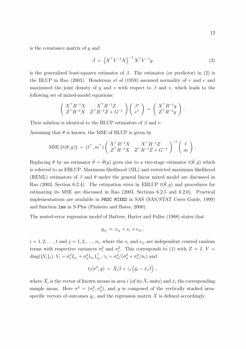
is the covariance matrix of y and

β =(X>V −1X

)−1X>V −1y (3)

is the generalized least-squares estimator of β. The estimator (or predictor) in (2) is

the BLUP in Rao (2003). Henderson et al (1959) assumed normality of v and e and

maximized the joint density of y and v with respect to β and v, which leads to the

following set of mixed-model equations:(X>R−1X X>R−1ZZ>R−1X Z>R−1Z + G−1

)(β∗

v∗

)=

(X>R−1yZ>R−1y

).

Their solution is identical to the BLUP estimators of β and v.

Assuming that θ is known, the MSE of BLUP is given by

MSE {t(θ, y)} = (`>, m>)

(X>R−1X X>R−1ZZ>R−1X Z>R−1Z + G−1

)−1 (`m

).

Replacing θ by an estimator θ = θ(y) gives rise to a two-stage estimator t(θ, y) which

is referred to as EBLUP. Maximum likelihood (ML) and restricted maximum likelihood

(REML) estimators of β and θ under the general linear mixed model are discussed in

Rao (2003, Section 6.2.4). The estimation error in EBLUP t(θ, y) and procedures for

estimating its MSE are discussed in Rao (2003, Sections 6.2.5 and 6.2.6). Practical

implementations are available in PROC MIXED in SAS (SAS/STAT Users Guide, 1999)

and function lme in S-Plus (Pinheiro and Bates, 2000).

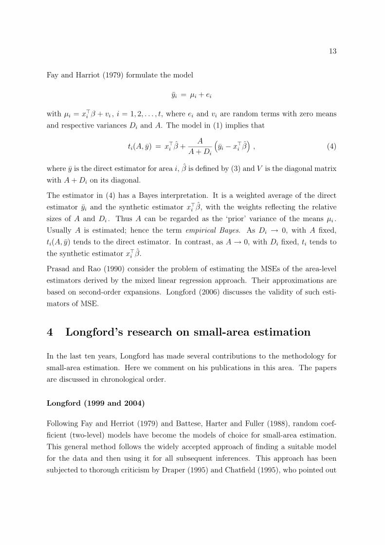
The nested-error regression model of Battese, Harter and Fuller (1988) states that

yij = xij + vi + eij ,

i = 1, 2, . . . , t and j = 1, 2, . . . , ni, where the vi and eij are independent centred random

terms with respective variances σ2v and σ2

e . This corresponds to (1) with Z = I, V =

diag({Vi}i), Vi = σ2eIni

+ σ2u1ni

1>ni, γi = σ2

u/(σ2u + σ2

e/ni) and

ti(σ2, y) = Xiβ + γi

(yi − xiβ

),

where Xi is the vector of known means in area i (of its Ni units) and xi the corresponding

sample mean. Here σ2 = (σ2e , σ2

u), and y is composed of the vertically stacked area-

specific vectors of outcomes yi , and the regression matrix X is defined accordingly.

13

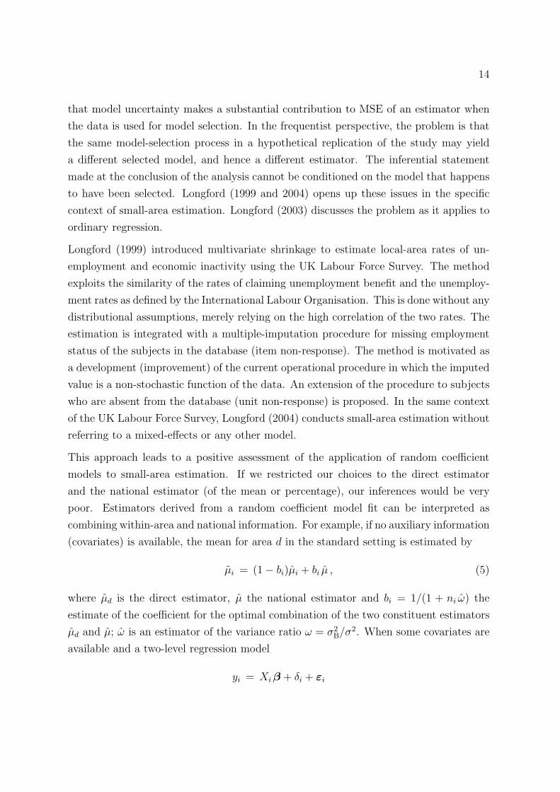
Fay and Harriot (1979) formulate the model

yi = µi + ei

with µi = x>i β + vi , i = 1, 2, . . . , t, where ei and vi are random terms with zero means

and respective variances Di and A. The model in (1) implies that

ti(A, y) = x>i β +A

A + Di

(yi − x>i β

), (4)

where y is the direct estimator for area i, β is defined by (3) and V is the diagonal matrix

with A + Di on its diagonal.

The estimator in (4) has a Bayes interpretation. It is a weighted average of the direct

estimator yi and the synthetic estimator x>i β, with the weights reflecting the relative

sizes of A and Di . Thus A can be regarded as the ‘prior’ variance of the means µi .

Usually A is estimated; hence the term empirical Bayes. As Di → 0, with A fixed,

ti(A, y) tends to the direct estimator. In contrast, as A → 0, with Di fixed, ti tends to

the synthetic estimator x>i β.

Prasad and Rao (1990) consider the problem of estimating the MSEs of the area-level

estimators derived by the mixed linear regression approach. Their approximations are

based on second-order expansions. Longford (2006) discusses the validity of such esti-

mators of MSE.

4 Longford’s research on small-area estimation

In the last ten years, Longford has made several contributions to the methodology for

small-area estimation. Here we comment on his publications in this area. The papers

are discussed in chronological order.

Longford (1999 and 2004)

Following Fay and Herriot (1979) and Battese, Harter and Fuller (1988), random coef-

ficient (two-level) models have become the models of choice for small-area estimation.

This general method follows the widely accepted approach of finding a suitable model

for the data and then using it for all subsequent inferences. This approach has been

subjected to thorough criticism by Draper (1995) and Chatfield (1995), who pointed out

14

that model uncertainty makes a substantial contribution to MSE of an estimator when

the data is used for model selection. In the frequentist perspective, the problem is that

the same model-selection process in a hypothetical replication of the study may yield

a different selected model, and hence a different estimator. The inferential statement

made at the conclusion of the analysis cannot be conditioned on the model that happens

to have been selected. Longford (1999 and 2004) opens up these issues in the specific

context of small-area estimation. Longford (2003) discusses the problem as it applies to

ordinary regression.

Longford (1999) introduced multivariate shrinkage to estimate local-area rates of un-

employment and economic inactivity using the UK Labour Force Survey. The method

exploits the similarity of the rates of claiming unemployment benefit and the unemploy-

ment rates as defined by the International Labour Organisation. This is done without any

distributional assumptions, merely relying on the high correlation of the two rates. The

estimation is integrated with a multiple-imputation procedure for missing employment

status of the subjects in the database (item non-response). The method is motivated as

a development (improvement) of the current operational procedure in which the imputed

value is a non-stochastic function of the data. An extension of the procedure to subjects

who are absent from the database (unit non-response) is proposed. In the same context

of the UK Labour Force Survey, Longford (2004) conducts small-area estimation without

referring to a mixed-effects or any other model.

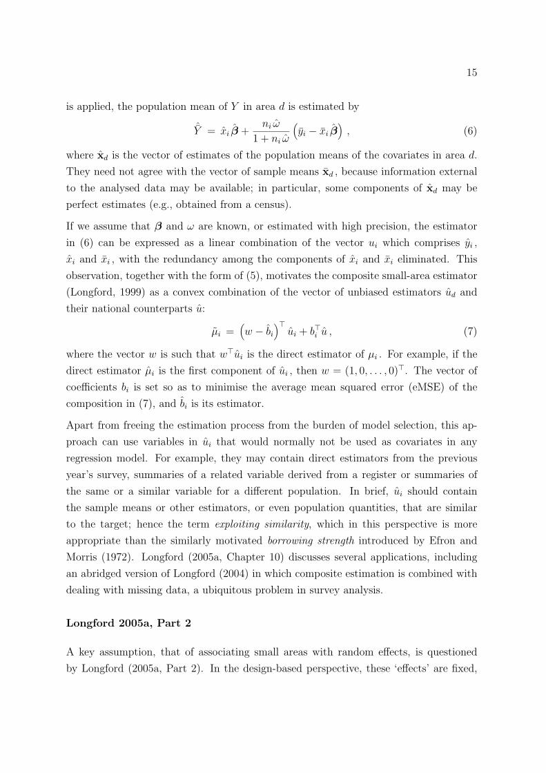
This approach leads to a positive assessment of the application of random coefficient

models to small-area estimation. If we restricted our choices to the direct estimator

and the national estimator (of the mean or percentage), our inferences would be very

poor. Estimators derived from a random coefficient model fit can be interpreted as

combining within-area and national information. For example, if no auxiliary information

(covariates) is available, the mean for area d in the standard setting is estimated by

µi = (1− bi)µi + bi µ , (5)

where µd is the direct estimator, µ the national estimator and bi = 1/(1 + ni ω) the

estimate of the coefficient for the optimal combination of the two constituent estimators

µd and µ; ω is an estimator of the variance ratio ω = σ2B/σ2. When some covariates are

available and a two-level regression model

yi = Xi β + δi + εi

15

is applied, the population mean of Y in area d is estimated by

ˆY = xi β +ni ω

1 + ni ω

(yi − xi β

), (6)

where xd is the vector of estimates of the population means of the covariates in area d.

They need not agree with the vector of sample means xd , because information external

to the analysed data may be available; in particular, some components of xd may be

perfect estimates (e.g., obtained from a census).

If we assume that β and ω are known, or estimated with high precision, the estimator

in (6) can be expressed as a linear combination of the vector ui which comprises yi ,

xi and xi , with the redundancy among the components of xi and xi eliminated. This

observation, together with the form of (5), motivates the composite small-area estimator

(Longford, 1999) as a convex combination of the vector of unbiased estimators ud and

their national counterparts u:

µi =(w − bi

)>ui + b>i u , (7)

where the vector w is such that w>ui is the direct estimator of µi . For example, if the

direct estimator µi is the first component of ui , then w = (1, 0, . . . , 0)>. The vector of

coefficients bi is set so as to minimise the average mean squared error (eMSE) of the

composition in (7), and bi is its estimator.

Apart from freeing the estimation process from the burden of model selection, this ap-

proach can use variables in ui that would normally not be used as covariates in any

regression model. For example, they may contain direct estimators from the previous

year’s survey, summaries of a related variable derived from a register or summaries of

the same or a similar variable for a different population. In brief, ui should contain

the sample means or other estimators, or even population quantities, that are similar

to the target; hence the term exploiting similarity, which in this perspective is more

appropriate than the similarly motivated borrowing strength introduced by Efron and

Morris (1972). Longford (2005a, Chapter 10) discusses several applications, including

an abridged version of Longford (2004) in which composite estimation is combined with

dealing with missing data, a ubiquitous problem in survey analysis.

Longford 2005a, Part 2

A key assumption, that of associating small areas with random effects, is questioned

by Longford (2005a, Part 2). In the design-based perspective, these ‘effects’ are fixed,

16

because a hypothetical replication of the survey would yield exactly the same population,

with the same division to areas; the sampling process is the only source of variation.

The problematic nature of the assumption of random effects can be illustrated by a

simple simulation in which estimators are applied to the samples drawn from an artificial

population. It shows that the estimation for the areas that have means close to the

national mean is more precise and for those that have means distant from the national

mean is less precise than indicated by the formula offered by the random-effects model.

This formula is nevertheless useful as an indicator of the average MSE, although the

qualifier ‘average’ has to be understood as an expectation over the distribution of the

area-level deviations, not as a simple averaging over the areas that have the same or

similar sample sizes.

Longford (2005a) derives conditions for an auxiliary variable to be useful: high corre-

lation of its area-level population means with the targets, small sampling variance, and

small correlation with the population means of the other auxiliary variables. Notably,

they differ from the conditions for a good model fit (reduction of the variance components

in the random-effects model). This suggests that the standard approach of identifying a

well fitting model, and then basing all inferences on it, is suboptimal.

Longford 2005b

Longford (2005b) discusses the issue of estimating many quantities and using the esti-

mates by clients not involved in the estimation process. It highlights the problem that

when an estimator is used conditionally (is selected for reporting based on its value), its

properties should also be evaluated with the condition applied. A related problem is that

a target is selected after inspecting an extensive list of estimates. The properties of such

an estimator differ from the properties of the same estimator if it were selected uncon-

ditionally; that is, the selection process is non-ignorable. Also, a collection of estimators

that are efficient for their respective targets need not have the same good properties

when their precisions are summarized in a different way.

Longford, 2006a

Most large-scale (national) surveys have a wide inferential agenda, and their design rarely

takes the preferences for small-area estimation into account. Longford (2006a) presents

17

a framework in which such preferences, or inferential priorities, for small-area estimation

can be taken into account in the design of a survey. He describes a general approach to

setting the sampling design in surveys that are planned for making inferences about small

areas (sub-domains). The approach requires a specification of the inferential priorities

for the areas. The methods are illustrated on an example of planning a survey of the

population of Switzerland and estimating the mean or proportion of a variable for each

of the country’s 26 cantons.

Longford 2006b

Small-area estimation is a quintessentially small-sample problem, and so asymptotic

results do not apply to it. In particular, an efficient estimator θi of a quantity θi loses its

good properties by transformations. For instance, θ2i is not an efficient estimator of θ2

i .

A related example, of allocating limited funds to small areas is discussed in the paper.

Composite estimation is shown to be rather inefficient for this purpose, even though it

would be efficient if θd were the target, without any nonlinear transformation. Any other

estimator has the same deficiency.

Longford, 2007

Longford (2007) argues that the design-based perspective is ‘correct’ and the assumption

made for random coefficient models is opportunistic, to enable borrowing strength and

avoid the inability of design-based methods to exploit the auxiliary information. The

model-based methods are suitable for estimation of the small-area quantities, but not for

estimation of the associated standard errors. Longford (2007) illustrates this on a general

example and proposes an estimator of the MSE that is itself based on composition.

5 Other recent papers on small-area estimation

Khoshgooyanfard and Monazzah, 2006

In this paper, a synthetic, a composite and the empirical Bayes estimators are compared

in the context of estimating unemployment rates for the provinces of Iran. The three

estimators are compared by their MSEs assuming that complete data (enumeration) is

available for the year 1996. The paper develops a proposal for a cost-effective strategy

18

to estimate the intercensal unemployment rate at the provincial level. The findings

indicate that the composite and empirical Bayes estimators perform well and similarly

to one another. The study assumes that the true values are known from a Census. Only

one replicate is considered in the experimental exercise.

You and Chapman, 2006

A full hierarchical Bayes (HB) model is constructed for the small-area estimators and

for estimating their sampling variances. The Gibbs sampler is employed to obtain the

small-area HB estimators. It is found that the uncertainty about the model variances

does not affect the small-area estimators, althought it has some minor impact on the

estimation of standard errors.

In the Fay-Herriot model (Fay and Herriot, 1979), we have the following two equations

θi = x>i β + vi

yi = θi + ei

(i = 1, 2, . . . ,m), with the variances σ2v and σ2

e of the between- and within-area deviations.

The two equations can be combined as

yi = x>i β + vi + ei .

The variance σ2e usually has the form σ2

i /ni , where ni is the subsample size in area i. The

variance σ2i is estimated by the sample variance s2

i of these ni observations. A combined

estimator s2 for σ2i could be constructed by pooling all the s2

i with weights proportional

to the sample sizes ni , suitably adjusted for the lost degrees of freedom. This model can

be fitted by iteratively reweigthed least squares, with σ2v estimated. You and Chapman

(2006) explore the alternatives to using the Gibbs sampler for fitting the Fay-Herriot

model.

6 Conclusions

Our review suggests that, depending on the available information, there are two avenues

that can be pursued in small-area estimation: methods free of any covariates and meth-

ods that make use of auxiliary variables (covariates). The IDESCAT-UPF research on

small-area estimation has concentrated on the first avenue. Research concentrated on

19

design issues and on comparing the efficiency of alternative small-area estimators. This

relatively narrow focus of the team IDESCAT-UPF is in accord with the view that official

statistics should be free of the subjectivity that might be introduced by the uncertainties

of model specification (e.g., the choice of covariates).

Covariates can be handled by mixed-effects regression. A clear limitation of such an

approach to small-area estimation in official statistics is that the choice of the covariates

injects some arbitrariness into the data production (beyond and above sampling fluctu-

ation) that is alien to the established ethos of official statistics. Further, a fundamental

assumption of the mixed-effects regression is that covariates are free from measurement

error. Uncertainty in the model specification has been subjected to criticism by Longford

(2003 and 2005a, Chapter 11).

The paper CSV06 has, however, gone beyond a single source of information. It has

integrated information from two surveys, producing small-area estimates that combine

information (borrow strength) from these two source of information, as well as from

neighboring areas. This approach is fundamentally different from the mixed-effects

model, in that no covariates are involved in the analysis. The approach is closer to

the multivariate setting in which correlated variables, both differing from their targets

(true values) by some error due to estimation, are combined into a single estimator.

Extensions to more than two sources of information are straightforward.

We have reviewed various methodological approaches to small-area estimation: design-

vs. model-based methods; the perspective free of model specification advocated by recent

work of Longford vs. the mixed-effects regression. Our methodological research has so

far integrated several of these perspectives, without involving any covariates. Given the

current state of research, it is advisable that the team IDESCAT-UPF concentrates on:

a) assisting in technical issues in the implementation of of standard methods for small-

area estimation to surveys currently undertaken by IDESCAT, such as the TIC

survey;

b) continuing the methodological research on small-area estimation, anchored to ‘real-

life’ problems and settings in official statistics.

An extension of the methodological work carried out by the IDESCAT-UPF team inte-

grates multivariate analysis and small-area estimation, possibly with the help of a flexible

modelling machinery, such as structural equation models for multilevel data.

20

7 References

Battese, G. E., Harter, R. M., and Fuller, W. A. (1988). An error components model

for prediction of county crop areas using survey and satellite data. Journal of the

American Statistical Association, 83, 28–36.

Clar, M., Ramos, R., and Surinach, J. (2000). Avantatges i inconvenients de la metodolo-

gia del INE per elaborar indicadors de la produccio industrial per a les regions es-

panyoles. Questiio, 264, 151–186.

Costa, A. and Galter, J. (1994). LIPPI, un indicador molt valuos per mesurar lactivitat

industrial catalana. Revista dIndustria, 3, Generalitat de Catalunya, 6-15.

Costa, A., Garcia, M., Lopez, X., and Pardal, M. (2006). Estimacio de les taxes de

desocupacio comarcal a Catalunya. Aplicacio d’estimadors de petita area amb com-

binacio d’enquestes. Working Document, IDESCAT, Barcelona.

Costa, A., Satorra, A., and Ventura, E. (2002). Estimadores compuestos en estadıstica

regional: aplicacion para la tasa de variacion de la ocupacion en la industria. Questiio,

26, 213–243.

Costa, A., Satorra, A., and Ventura, E. (2003). An empirical evaluation of small area

estimators. SORT (Statistics and Operations Research Transactions), 27, 113–135.

Costa, A., Satorra, A., and Ventura, E. (2004). Using composite estimators to improve

both domain and total area estimation. SORT (Statistics and Operations Research

Transactions), 28, 69–86.

Costa, A., Satorra, A., and Ventura, E. (2006). Improving small area estimation by

combining surveys: new perspectives in regional statistics. SORT (Statistics and

Operations Research Transactions), 30, 101–122.

Chatfield, C. (1995). Model uncertainty, data mining and statistical inference. Journal

of the Royal Statistical Society, Ser. A 158, 419–466.

Draper, D.(1995). Assessment and propagation of model uncertainty. Journal of the

Royal Statistical Society, Ser. B 57, 45–97.

Efron, B., and Morris, C. (1972). Limiting the risk of Bayes and empirical Bayes es-

timators — Part II: The empirical Bayes case. Journal of the American Statistical

Association, 67, 130–139.

Efron, B., and Morris, C. (1973). Stein’s estimation rule and its competitors — an

empirical Bayes approach. Journal of the American Statistical Association, 68, 117–

21

130.

Efron, B., and Morris, C (1975). Data analysis using Stein’s estimator and its general-

izations. Journal of the American Statistical Association, 70, 311–319.

Ericksen, E. (1973). A method of combining sample survey data and symptomatic

indicators to obtain population estimates for local areas. Demography, 10, 147–160.

Ericksen, E. (1974). A regression method for estimating population changes of local

areas. Journal of the American Statistical Association, 69, 867–875.

Fay, R. E., and Herriot, R. A. (1979). Estimates of income for small places: an applica-

tion of James-Stein procedures to census data. Journal of the American Statistical

Association, 74, 269–277.

Ghosh, M., and Rao, J. N. K. (1994). Small area estimation: an appraisal. Statistical

Science, 9, 55–93.

Henderson, C.R. (1975). Best Linear Unbiased Estimation and Prediction Under a

Selection Model, Biometrics, 31, 423-447

Henderson, C.R., Kempthorne, O., Searle, S.R. , and von Krosigh, C.N. (1959). Es-

timation of Environmental and Genetic Trends from Records Subject to Culling,

Biometrics, 13, 192-218

Isaki, C. T. (1990). Small-area estimation of economic statistics. Journal of Business &

Economic Statistics, 8, 435–441.

Jiang, J., and Lahiri, P. (2006). Mixed model prediction and small area estimation.

Test, 15, 1–96.

Jiang, J., and Lahiri, P. (2006). Estimation of finite po0pulation domain means — model

assisted empirical Bayes prediction approach. Journal of the American Statisical

Association, 101. In press.

Khoshgooanfard, A. R., and Monazzah, M. T. (2006). A cost-effective strategy for

provincial unemployment estimation: a small area approach. Survey Methodology

32, 105–114.

Longford, N. T. (1999). Multivariate shrinkage estimation of small area means and

proportions. Journal of the Royal Statistical Society, Ser. A 162, 227–245.

Longford N. T. An alternative to model selection in ordinary regression. Statistics and

Computing 13 67–80, 2003.

Longford, N. T. (2004). Missing data and small-area estimation in the UK Labour Force

22

Survey. Journal of the Royal Statistical Society Ser. A 167, 341–373.

Longford, N. T. (2005a). Missing Data and Small-Area Estimation: Modern Analytical

Equipment for the Survey Statistician. Springer-Verlag, New York.

Longford, N. T. (2005b). On selection and composition in small area and mapping

problems. Statistical Methods in Medical Research 14, 1–14.

Longford, N. T. (2006a). Sample size calculation for small-area estimation. Survey

Methodology 32, 87–96.

Longford, N. T. (2006b). Using small-area estimation. Statistics in Transition 7, 715–

735.

Longford, N. T. (2007). On standard errors of model-based small-area estimators. Survey

Methodology 33. In press.

Pinheiro, J. C., and Bates, D. (2000). Mixed-Effects Models in S and S-plus. Springer-

Verlag, New York.

Platek, R., Rao, J. N. K., Sarndal, C. E., and Singh, M. P. (Eds.) (1987). Small Area

Statistics: An International Symposium. John Wiley and Sons, New York.

Prasad, N. G. N., and Rao, J. N. K. (1990). The estimation of the mean squared error of

small-area estimators. Journal of the American Statistical Association, 85, 163–171.

Rao, J. N. K. (2003). Small Area Estimation. Wiley Series in Survey Methodology, New

York.

Singh, M. P., Gambino, J., and Mantel, H. J. (1994). Issues and strategies for small-area

data. Survey Methodology, 20, 3–22.

Santamarıa, L., Morales, D., and Molina, I. (2004). A comparative study of small area

estimators. SORT, 28, 215–230.

SAS/STAT (1999). User’s Guide, Vol. 2, SAS Institute, Cary, North Carolina.

StataCorp. (2003). Stata Statistical Software: Release 8.0. Stata Corporation, College

Station, TX.

You, Y., and Chapman, B. (2006). Small area estimation using area level models and

estimated sampling variances. Survey Methodology 32, 97–103.