SMHI HYDROLOGY No 481994 12000 10000 8000 6000 4000 2000 20 TEMPER A TUREl 'C INFLOW ! ni3/s ) APPLICATION OF THE HBV MODEL TO THE UPPER INDUS RIVER SNOW PAC K!mm FOR INFLOW FORECASTING TO THE TARBELA DAM Håkan Sanner, Joakim Harlin and Magnus Persson 20 10 0 -10 - 20 200
Transcript
SMHI HYDROLOGY No 481994
12000
10000
8000
6000
4000
2000
20
TEMPER ATUREl'C
INFLOW !ni3/s)
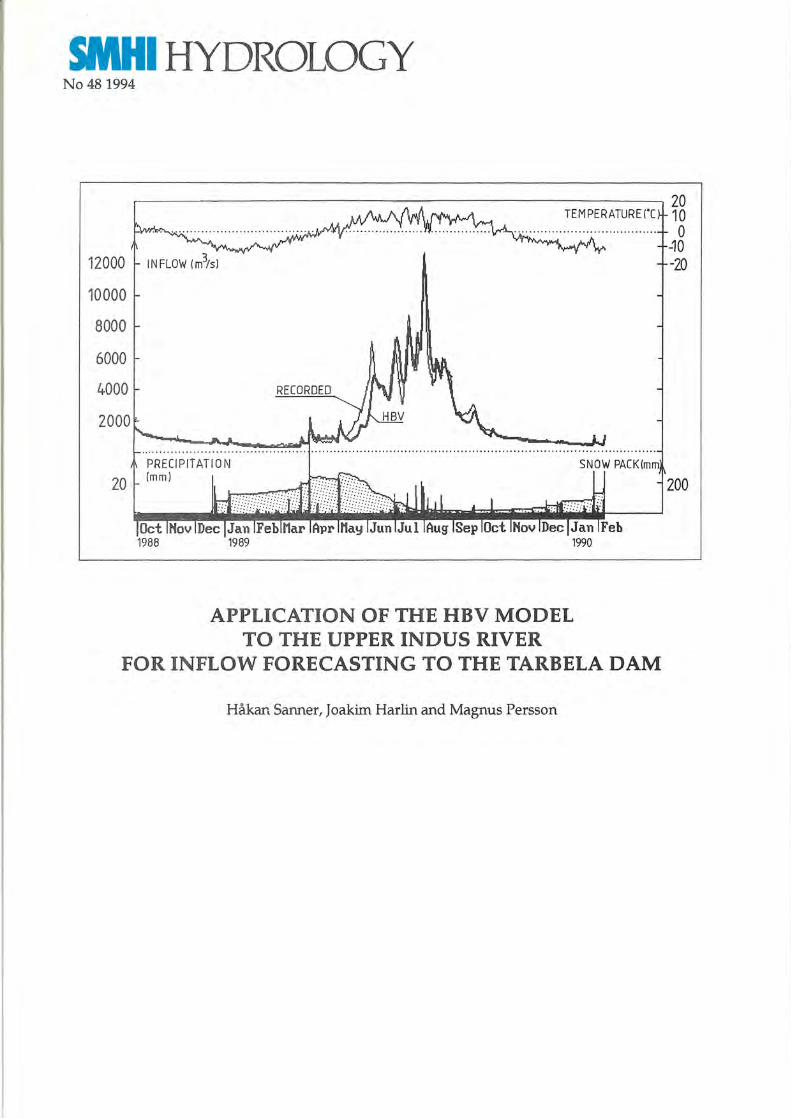
APPLICATION OF THE HBV MODEL TO THE UPPER INDUS RIVER
SNOW PACK!mm
FOR INFLOW FORECASTING TO THE TARBELA DAM
Håkan Sanner, Joakim Harlin and Magnus Persson
20 10 0
-10 -20
200
WHYDROLOGY
BIBLIOTEKET
APPLICA TION OF THE HBV MODEL TO THE UPPER INDUS RIVER
Appendix A: Double mass plots of the precipitation stations Appendix B: Conversion units for model input and output Appendix C: Calibration plots for the whole basin and the three subbasins
1. INTRODUCTION
This report describes the HBV model application for inflow forecasting on a daily time step to the Tarbela dam in the Indus River. The model application forms part of the new Tarbela control center for Pakistan's Water and Power Development Authority (W APDA). The new control system will be an ABB S.P.I.D.E.R. SCADA system, delivered on a turnkey basis by ABB Network Control of Sweden. SMHI have as subconsultants to the ABB Network Control been responsible for the set up, calibration, training and delivery of the inflow forecasting system based on the HBV model.
2. THE CLIMATE AND HYDROLOGY OF THE UPPER INDUS RIVER
The Upper Indus River catchment is about 1 100 (km) long with an average width of less than 160 (km), making a total catchment area of 173 000 (km2). The catchment is probably the highest basin in any river system, in this size, of the world. Within the Pakistan part of the catchment the highest peak is Mount Godwin Austen (K2) 8 611 (m.a.s.l). The climate is controlled by the system of Asian monsoons with two main seasons, the northeast monsoon and the southwest monsoon. The northeast monsoon begins in December and prevails until about the middle of March and brings dry and cool winds of moderate strength persistently out of the northeast from the Chinese mainland. The onset of the humid southwest monsoon is normally in mid July and the withdrawal date is in late October. This season accounts for the majority of the annual rainfall in the lower and mid parts of the Indus, and due to the orographic effect of the Siwalik Range and the Great Himalayas, also considerable amounts of rainfall to the Upper Indus. Local air temperatures vary a great deal within the Upper Indus mainly due to the large altitude effects. Mean daily temperatures, reduced to sea level, are for January 17 .5 - 20.0 (°C), April 30.0 (°C), July 30.0 - 32.5 (°C) and October 27 .5 (°C) (Takahashi and Arakawa, 1981 ).
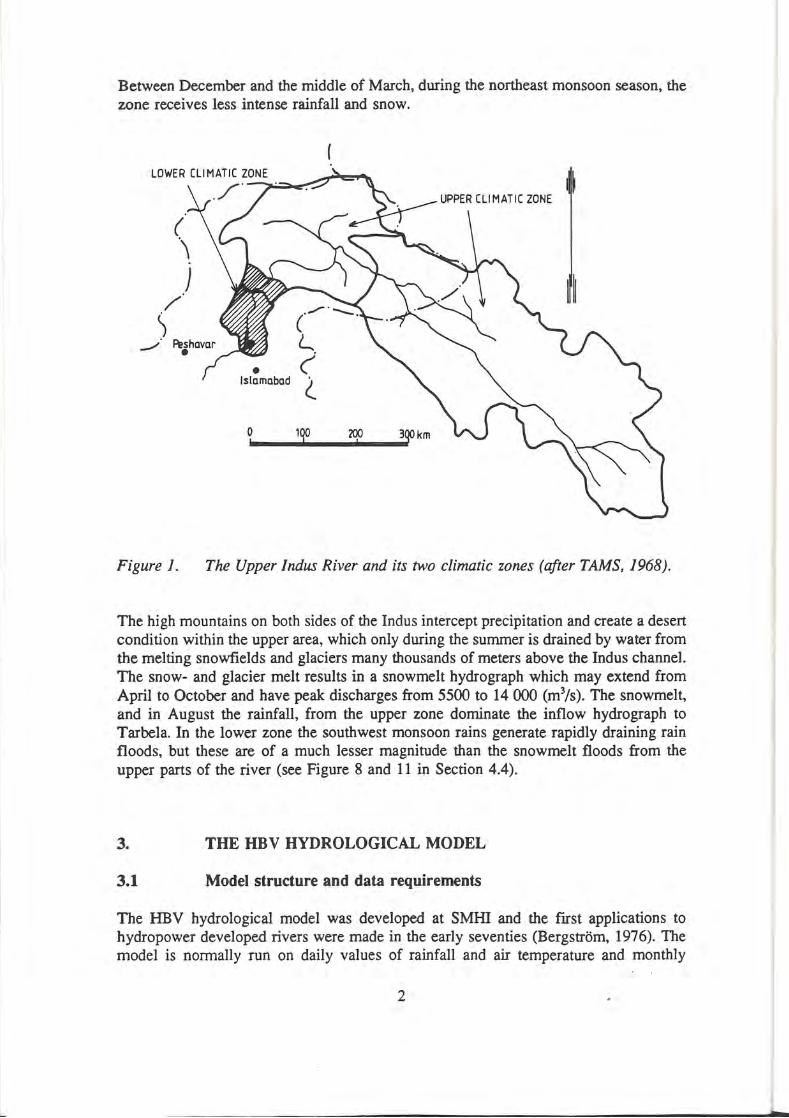
The Upper lndus River contains two climatic zones; the upper and the lower (see Figure 1). The upper zone, covering more than 90 % of the area, lies in an elongated northwest-southeast tending basin between the great mountain walls formed by the Karakoram Range in the north and the Great Himalayas Range in the south. It is the snowfields and glaciers in this region that feed the Indus with its perennial flows. The smaller zone, roughly a north-south rectangle at the lower end of the basin, lies between Tarbela and the area where the lndus River bends around the southern mountain wall and flows generally southward.
About one quarter of the Upper Indus catchment is occupied by continual snowfields and glaciers (T AMS, 1968). The continual snow line starts at about 4 270 (m.a.s.l). The higher altitudes of the Greater Himalayas receive large quantities of snow which feed more than 1000 glaciers, some of which are among the largest in the world. A vailable records indicate that annual precipitation at lower elevations in the upper zone, beginning at a point about 160 (km) upstream of Tarbela, is as small as 127 (mm). In the lower zone, heavy monsoon storms prevail in the latter half of the summer season.
1
Between December and the middle of March, during the northeast monsoon season, the zone receives less intense rainfall and snow.
LOWER CLIMAT IC ZONE
( \ )
/ ~
_./
./"
011111
___ 1qo_,_ __ 200._1
--3-QOkm
I ~
I Il
Figure 1. The Upper Indus River and its two climatic zones (after TAMS, 1968).
The high mountains on both sides of the Indus intercept precipitation and create a desert condition within the upper area, which only during the surnmer is drained by water from the melting snowfields and glaciers many thousands of meters above the Indus channel. The snow- and glacier melt results in a snowmelt hydrograph which may extend from April to October and have peak: discharges from 5500 to 14 000 (m3/s). The snowmelt, and in August the rainfall, from the upper zone dominate the inflow hydrograph to Tarbela. In the lower zone the southwest monsoon rains generate rapidly draining rain floods, but these are of a much lesser magnitude than the snowmelt floods from the upper parts of the river (see Figure 8 and 11 in Section 4.4).
3. THE HBV HYDROLOGICAL MODEL
3.1 Model structure and data requirements
The HBV hydrological model was developed at SMHI and the first applications to hydropower developed rivers were made in the early seventies (Bergström, 1976). The model is normally run on daily values of rainfall and air temperature and monthly
2
estimates of potential evapotranspiration. The model contains routines for snow accumulation and melt, soil moisture accounting, runoff generation and a simple routing procedure (Figure 2). It can be used in a distributed mode by dividing the catchment into subbasins. Each subbasin is then divided into zones according to altitude, lake area, glaciers and vegetation.
distributed snow rutine according to elevation ond vegetation
s., = snow storage in forest S00 = snow storage in open areas Sam = soil moisture storage Fe = max. soil water saz = storage in upper response tank UZL = limit for tbe quickest runoff
component Siz = storage in lower response tank Qo, Q1, Q2 = runoff components Ko, K1, K2 = recession components
Figure 2. The general structure of the HBV mode/ when applied to one subbasin.
3.1.1
Snowmelt is calculated separately for each elevation and vegetation zone according to the degree-day equation:
Q ,,i(t) = CFMAX · (T(t) - 77)
where:
<Jm CFMAX T TT
= snowmelt = degree-day factor = mean daily air temperature = threshold temperature for snowmelt.
(1)
Because of the porosity of the snow, some rain and meltwater can be retained in the pores. In the model, a retention capacity of 10 % of the snowpack water equivalent is assumed. Only after the retention capacity has filled, meltwater will be released from the snow. The snow routine also has a general snowfall correction factor (SFCF) which
3
adjusts for systematic errors in calculated snowfall and winter evaporation. Glacier melting is taken account of by the same type of formula as for snow melting, however, with a glacier specific degree-day factor (GMEL T). No glacier melting occurs as long as there is snow in the current elevation zone.
3.1.2 Soil moisture
Soil moisture dynamics are calculated separately for each elevation and vegetation zone. The rate of discharge of excess water from the soil is related to the weighted precipitation and the relationship depends upon the computed soil moisture storage, the soil saturation threshold (FC) and the empirical parameter ~. as given in equation 2. Rain or snowmelt generates small contributions of excess water from the soil when the soil is dry and large contributions when conditions are wet (Figure 3).
( Ssm(t)lp Q(t) = - • P(t)
s FC
(2)
where: (Js = excess water from soil Ssm = soil moisture storage FC = soil saturation threshold P = precipitation 13 = empirical coefficient
The acual evapotranspiration is computed as a function of the potential evapotranspiration and the available soil moisture (Eq. 3, Figure 3):
where:
if s_ s LP
if s_ > LP
Ea = actual evapotranspiration EP = potential evapotranspiration LP = Ssm threshold for Ep
4
(3)
Ssm • computed soil moisture storage tJ> • contribution from rainfall or snowmelt AQ • contribution to the response function Fe - maximum soil moisture storage {I - cmpirical coefficient EP - potential evapotranspiration
E8 - computed actual evapotranspiration
LP - limit for potential evapotranspiration
åQ/åP=(Ssm/Fc)~ Ea/EP
1.0 1.0
0.0 0.0
o.o Fe Ssm o.o
Figure 3. Schematic presentation of the soil moisture accounting subroutine.
3.1.3 Runoff response
Excess water from the soil and direct precipitation over open water bodies m the catchment area generate runoff according to equations (4) and (5).
Q.(t) {
where:
~ Ko, K1, K2 UZL suz PERC Q s1z
= Sw.(t) · (K0 + K1) - K0 • UZL
= Kl . S,it)
if SIIZ > UZL
if Suz :s: UZL
= runoff generation from upper response tank = recession coefficients = storage threshold between Ko and K1
= storage in upper response tank = percolation rate between the tanks = runoff generation from lower response tank = storage in lower response tank
(4)
(5)
In order to account for the damping of the generated flood pulse (Q = ~ + Q) in the river, a simple routing transformation is made. This isa filter with a triangular distribution of weights with the base length MAXBAS. There is also an option of using the Muskingum routing routine to account for the river flow hydraulics.
Lakes in the subbasins are included in the lower response tank, but can also be modelled explicitly by a storage discharge relationship. This is accomplished by subdivision into subbasins defined by the outlet of major lakes. The use of an explicit lake routing routine has also proved to simplify the calibration of the recession parameters of the model, as most of the damping is accounted for by the lakes.
5
3.2 Model applications
The HBV model was originally developed for inflow forecasting to hydropower reservoirs in Scandinavian catchments, but has now been applied in more than 30 countries all over the world (Figure 4). Despite its relatively simple structure, it performs equally well as the best known model in the world (see WMO, 1986 and 1987).
Some examples of model applications are: inflow and flood forecasting and computation of design floods in totally about 170 basins in Scandinavia (Häggström, 1989; Bergström et al., 1989; Harlin, 1992; Killingtveit and Aam, 1978; Vehviläinen, 1986), modelling the effects of clearcutting in Sweden (Brandt et al., 1988), snowmelt flood simulation in Alpine regions (Capovilla, 1990; Renner and Braun, 1990; Braun and Lang, 1986), hydrological modelling in Arctic permafrost environment (Hinzman and Kane, 1991) and flood forecasting in Central America (Häggström et al., 1990).
Figure 4.
3.3
0
Countries or regions where the HBV mode/ is known to have been applied (from Bergström, 1992).
Model calibration
The HBV model, in its simplest form with only one subbasin and one type of vegetation, has altogether 12 free parameters. The calibration of the model is usually made by a manual trial and error technique, during which relevant parameter values are changed until an acceptable agreement with observations is obtained. The judgement of the
6
performance is also supported by statistical criteria, normally the R2-value of model fit, -== explained variance, (Nash and Sutcliffe, 1970):
R2 = L (Qo - Qo)2 - I: (Qc - Qo)2 L (Q0 - Q0 ) 2
where: Cl, <l (Je
= observed runoff = mean of observed runoff = computed runoff
(6)
R2 has a value of 1.0, if the simulated and the recorded hydrographs agree completely, and 0 if the mode! only manages to produce the mean value of the runoff record. Another useful tool for the judgement of mode! performance is a graph of the accumulated difference between the simulated and the recorded runoff. This graph reveals any bias in the water balance and is often used in the initial stages of calibration, for example for assessment of the snow parameters (see for example Figure 8).
It is not possible to specify exactly the required length of records needed for a stable model calibration for all kinds of applications. The important thing is that the records include a variety of hydrological events, so that the effect of all subroutines of the model can be discerned. Normally 5 to 10 years of records are sufficient when the model is applied to Scandinavian conditions.
The HBV model is a conceptual mode! lumping many heterogeneous catchment characteristics into rather simple linear and nonlinear equations. Although model components clearly represent individual hydrological processes, flow-generating pulses should not be interpreted as emanating from exact locations in the catchment. The model formulation has been developed so that the integrated response of all flow pulses during a time step is captured. Parameter values are therefore integrated and specific for each catchment and can not easily be obtained from point measurements in the field.
3.4 The forecasting procedure
The HBV model is often used for either short or long range forecasting. Before the day of forecast the model is run on observed input data until the time step (day) before the forecast lf there is a discrepancy between the computed and observed hydrographs during the last days of run, updating of the model should be considered. The HBV model is normally updated by an iterative procedure during which the input data a few days prior to the day of forecast is adjusted. Updating should always be done with caution, since the updating procedure may introduce additional uncertainty over the forecast period.
Short range forecasts are usually made in flood situations. The runoff development is forecasted until the culmination has passed. A meteorological forecast is used as input,
7
and there is a possibility to use alternative precipitation and temperature sequences in the same run. This is often desirable due to the often low accuracy of quantitative meteorological forecasts, especially as concems precipitation.
Long range forecasts are mainly used for two purposes: prediction of peak flow and of runoff volume. For operating hydropower reservoirs, the remaining inflow to a given date is often the most interesting figure, while in other basins the interest is concentrated towards the distribution of peak flows. The latter aspect is, of course, the most important if flood damage is the rnain problem. On the other hand, for some rivers, low flow forecasts can be the most interesting ones. The forecast uses precipitation and temperature data from corresponding periods of preceding years as input. Usually data from at least 10 years are used. The distribution of different simulations gives an indication of the probability that a given value will be exceeded. The volume forecast is supplemented with a statistical interpretation of the result.
4. THE HBV MODEL APPLICATION TO THE TARBELA CATCHMENT
4.1 Basin subdivision
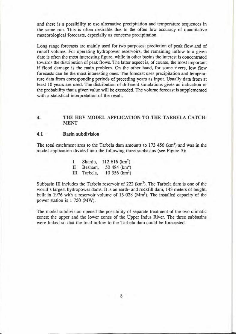
The total catchment area to the Tarbela dam amounts to 173 456 (knl) and was in the model application divided into the following three subbasins (see Figure 5):
I Skardu, Il Besham, 111 Tarbela,
112 616 (km2)
50 484 (km2)
10 356 (km2)
Subbasin 111 includes the Tarbela reservoir of 222 (km2). The Tarbela dam is one of the world's largest hydropower dams. It is an earth- and rockfill dam, 143 meters of height, built in 1976 with a reservoir volume of 13 028 (Mm3). The installed capacity of the power station is 1 750 (MW).
The model subdivision opened the possibility of separate treatment of the two climatic zones; the upper and the lower zones of the Upper Indus River. The three subbasins were linked so that the total inflow to the Tarbela dam could be forecasted.
8
,-J'./ ( \
INDIAN OCEAN
0 100
INDIA
Figure 5. The Tarbela catchment, basin subdivision and location ofprecipitation (P), temperature (T) and discharge stations (Q).
9
4.2 Analysis of input data
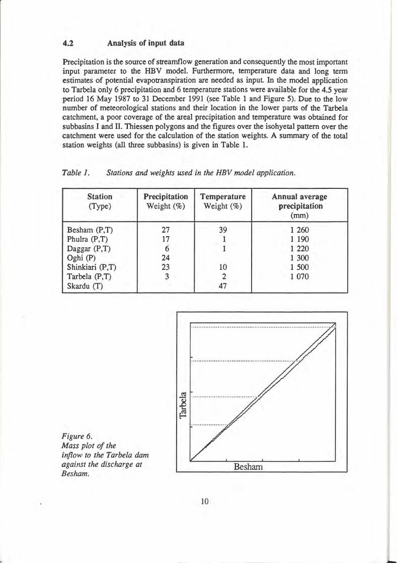
Precipitation is the source of streamflow generation and consequently the most important input parameter to the HBV model. Furthermore, temperature data and long term estimates of potential evapotranspiration are needed as input In the model application to Tarbela only 6 precipitation and 6 temperature stations were available for the 4.5 year period 16 May 1987 to 31 December 1991 (see Table 1 and Figure 5). Due to the low number of meteorological stations and their location in the lower parts of the Tarbela catchment, a poor coverage of the areal precipitation and temperature was obtained for subbasins I and Il. Thiessen polygons and the figures over the isohyetal pattem over the catchment were used for the calculation of the station weights. A summary of the total station weights (all three subbasins) is given in Table 1.
Table 1. Stations and weights used in the HBV modet application.
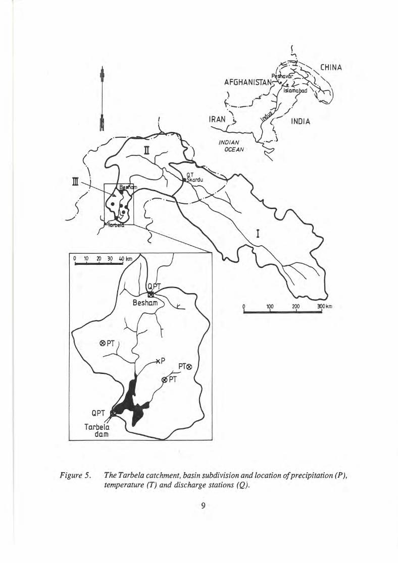
Figure 6. Mass plot of the inflow to the Tarbela dam against the discharge at Besham.
27 17 6
24 23 3
Temperature Annual average Weight (%) precipitation
(mm)
39 1 260 1 1 190 1 1 220
1 300 10 1 500 2 1 070
47
Besham
10
-
When analysing the inflow/discharge data it was found that the recorded inflow to the Tarbela dam was of smaller magnitude than the recorded discharge at Besham, although Tarbela has a greater cåtchment area. Figure 6 shows the mass plot between Tarbela and Besham. Observe that the Tarbela inflow lies below the diagonal, i.e. is of smaller magnitude than Besham. This fäet is probably due to measurement errors. During the calibration, the HBV model was thus tuned against the inflow data to the Tarbela reservoir which explains the poor volume perf ormance of the model output when compared with the Besham data (see Figure 3, Appendix C).
The double mass technique was used to check the homogeneity of the precipitation and discharge records. This technique takes advantage of the fäet that the mean accumulated precipitation for a number of gauges is not very sensitive to changes at individual stations because many of the errors compensate each other, whereas the cumulative curve for a single gauge is immediately affected by a change at the station.
The mean accumulated precipitation for all other stations is plotted on the X-axis against that for the gauge being studied, which is plotted on the Y-axis. lf the double mass curve has a change in slope at some point in time, it indicates a break in homogeneity. A jag in the double mass curve can be caused by rnissing values at the observed station or by seasonal differences in the precipitation pattern. The slope of the curve is proportional to the intensity, i.e. if the observed station records exactly as much as the mean of the rest, the curve follows the diagonal. lf the station records more, the slope will be steeper and if it records less, the double mass curve will lie below the diagonal.
The double mass curves for the stations at Besham and Tarbela (Appendix A) showed signs of inhomogeneity. The low number of stations and the short periods available did, however, not give any possibility to analyse the data quality any further. No corrections within the data periods were thus applied.
Monthly mean values of potential evapotranspiration were compiled from available evaporimeter pans of the Class A type, situated within the lower parts of the river basin. For the subbasins above Besham (I and Il) no evaporation observations were available. In the model application the evaporation data from the Tarbela subbasin was used, reduced to 50 % in order to compensate for the change in clirnatic regime (UNESCO, 1978), shallower soils, topography and to obtain a correct water balance. The potential evapotranspiration values for the three subbasins are given in Table 2.
Table 2.
Subbasin
I Skardu
Mean potential evapotranspiration (mmlday) data used in the HBV mode! application.
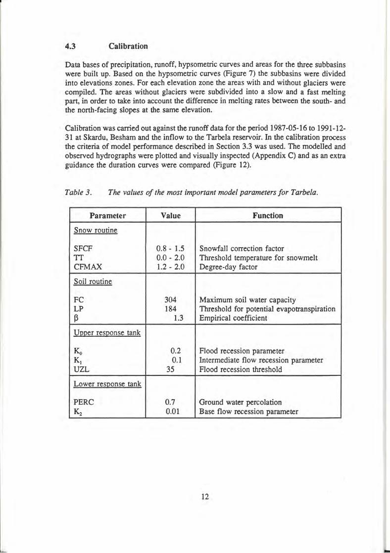
Data bases of precipitation, runoff, hypsometric curves and areas for the three subbasins were built up. Based on the hypsometric curves (Figure 7) the subbasins were divided into elevations zones. For each elevation zone the areas with and without glaciers were compiled. The areas without glaciers were subdivided into a slow and a fast melting part, in order to take into account the diff erence in melting rates between the south- and the north-facing slopes at the same elevation.
Calibration was carried out against the runoff data for the period 1987-05-16 to 1991-12-31 at Skardu, Besham and the inflow to the Tarbela reservoir. In the calibration process the criteria of model performance described in Section 3.3 was used. The modelled and observed hydrographs were plotted and visually inspected (Appendix C) and as an extra guidance the duration curves were compared (Figure 12).
Table 3. The values of the most important mode! parameters for Tarbela.
Parameter Value Function
Snow routine
SFCF 0.8 - 1.5 Snowfall correction factor TI 0.0 - 2.0 Threshold temperature for snowmelt CFMAX 1.2 - 2.0 Degree-day factor
Soil routine
FC 304 Maximum soil water capacity LP .184 Threshold for potential evapotranspiration ·
PERC 0.7 Ground water percolation K2 0.01 Base flow recession parameter
12
-
-- --• .,oo
t IO .0 N to 100 0 H.OIOto100
• •
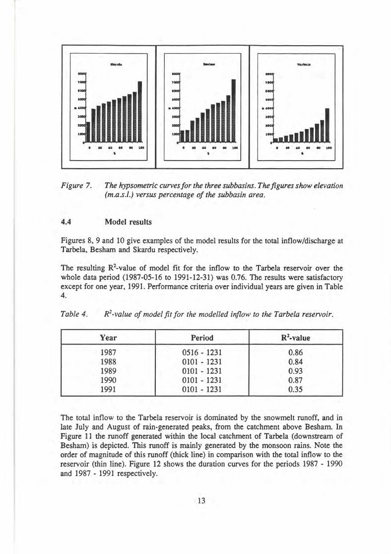
Figure 7. The hypsometric curvesfor the three subbasins. Thefigures show elevation (m.a .s./.) versus percentage of the subbasin area.
4.4 Model results
Figures 8, 9 and 10 give examples of the model results for the total inflow/discharge at Tarbela, Besham and Skardu respectively.
The resulting R2-value of model fit for the inflow to the Tarbela reservoir over the whole data period (1987-05-16 to 1991-12-31) was 0.76. The results were satisfactory except for one year, 1991. Perf ormance criteria over individual years are given in Table 4.
Table 4. R2-value of mode! fit for the modelled inflow to the Tarbela reservoir.
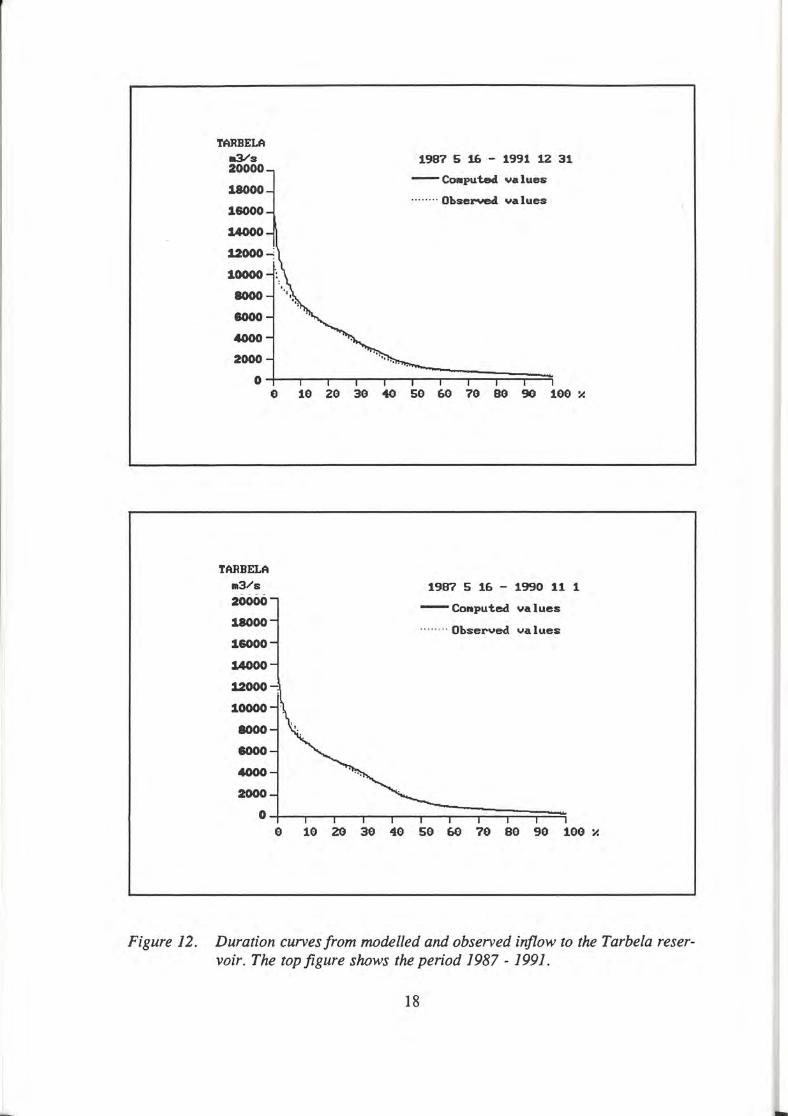
The total inflow to the Tarbela reservoir is dominated by the snowmelt runoff, and in late July and August of rain-generated peaks, from the catchment above Besham. In Figure 11 the runoff generated within the local catchment of Tarbela (downstream of Besham) is depicted. This runoff is mainly generated by the monsoon rains. Note the order of magnitude of this runoff (thick line) in comparison with the total inflow to the reservoir (thin line). Figure 12 shows the duration curves for the periods 1987 - 1990 and 1987 - 1991 respectively.
p 280 SP •miw.._.._...._._ ....... ,...~_....i..-iiijiiii~~~~.w.-...._..__. ____ _J ••
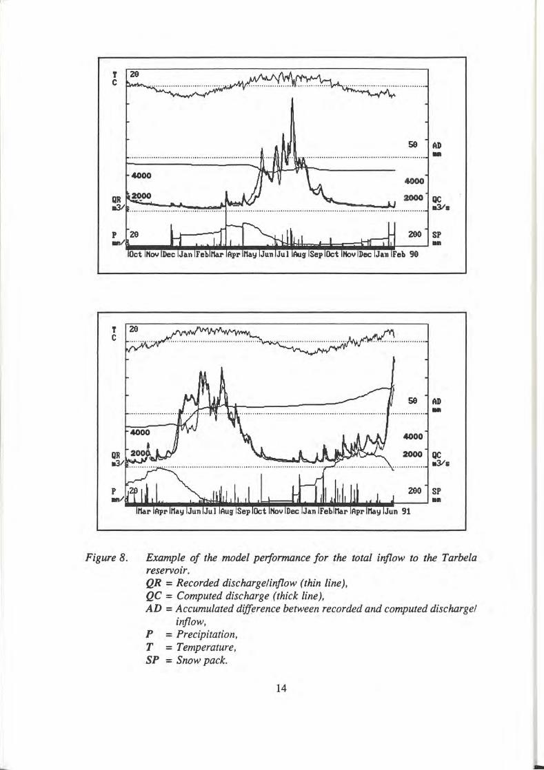
Figure 8. Example oj the mode/ pe,formance for the total inflow to the Tarbela reservoir. QR = Recorded discha.rgelinflow (thin line), QC = Computed discha.rge (thick fine), AD = Accumulated dijference between recorded and computed discha.rge/
inflow, P = Precipitation, T = Temperature, SP = Snow pack.
M •il..,.,_.-... liilliillil...r.WWiiiiiiiåa-.. iwi1111iM.-•lliMI-----'•
Figure 9. Example of the mode/ peiformance for the total discharge at Besham. QR = Recorded dischargelinflow (thin fine), QC = Computed discharge (thick fine), AD = Accumulated difference between recorded and computed dischargel
inflow, P = Precipitation, T = Temperature, SP = Snow pack.
Figure JO. Example of the mode! pe,formance for the total discharge at Skardu. QR = Recorded dischargelinflow (thin fine), QC = Computed discharge (thick fine), AD = Accumulated difference between recorded and computed discharge/
inflow, P = Precipitation, T = Temperature, SP = Snow pack.
16
T C
T C
QJl 1131
58 AD .. 4000
2000 QC 1131•
280 SP ..
58 AD • Il
4000 4000
2000 QC •3/s
280 SP
iiili~..,..~---~~lliij-........ -.-ii~..-.~iliilil ......... lillill!llllil"---:--:--___,1 • Il
Figure 11. The computed runoff generated in the local catchment area to Tarbela (below Besham) compared with the total recorded inflow to the reservoir. QR = Recorded dischargelinflow (thin fine), QC = Computed discharge (thick fine), AD = Accumulated difference between recorded and computed discharge/
inflow, P = Precipitation, T = Temperature, SP = Snow pack.
17
TARBELA 113/s 20000
18000
16000
14000
12000--:
10000
8000
6000
4000
2000
1987 5 16 - 1991 12 31
- C011putecl Ya lues
· .. · .. · · Ohsel'Yed Ya lues
0 .L-...--..-----.--..--~::=:::::;:::::;::=::;=;
TARBELA 113/s
20000
18000
16000
14000
8 18 20 30 40 50 60 70 BO 90 100 ~
1987 5 16 - 1990 11 1
-Conputed. Yalues
.. . ..... Ohserved Ya lues
12000:
10000
8000
6000
4000
2000
0 0 10 20 30 40 50 &O 70 BO 90 100 ~
Figure 12. Duration curves from mode/led and observed inflow to the Tarbela reservoir. The top figure shows the period 1987 - 1991.
18
5. DISCUSSION AND CONCLUSIONS
The HBV mode! application to the Tarbela catchment is, to the authors knowledge, the largest catchment area for which the HBV mode! so far has been applied, and probably also the catchment with the highest elevation span. Despite the poor coverage of precipitation and temperature input data, the HBV mode! was able to describe more than 75 % of the variance of the inflow to the Tarbela reservoir.
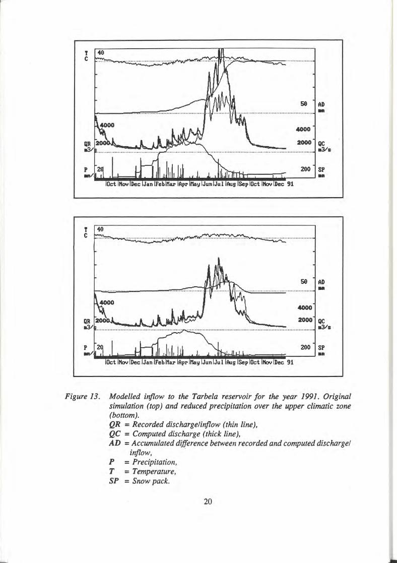
The poorest model performance was the one for the 1991 year flood. For this flood the model overestimated the runoff volume. This year, the utilized precipitation stations, mainly located in the Tarbela subbasin, were not representative of the precipitation over the upper climatic zone (mainly located within India). In Figure 13, a comparison is shown between the original mode! run and a run in which the precipitation over the upper climatic zone has been rescaled. The model performance reveals that if precipitation data for the upper climatic zone had been available, the overestimation in 1991 would probably have been avoided.
It is our opinion that the model application could be considerably improved if more input data were made available. It may be difficult to receive data for the upper climatic zone in real time. However, further precipitation and temperature data are available within Pakistan, e.g. from Gilgit, Astore and Chilas. lf these data also bad been used, an almost certain mode! improvement would have resulted.
In conclusion the HBV mode! application to the Tarbela catchment has shown that:
• The HBV model can simulate the hydrology of the Upper Indus with a good model performance despite the small input data quantity.
• The model responded at all flood events in the available data period, however, not always with the correct flood magnitude. Consequently, early flood warning from the HBV mode! should be taken seriously.
• The model performance is equally good for the Upper Indus down to Skardu, as for the total catchment to the Tarbela dam.
• The catchment has a quick response to rainfall, often only 24 hours.
• The largest floods are generated by rainfall events during or at the end of the snowmelt period.
• lf real time precipitation and temperature data as well as an accurate meteorological forecast is available, the HBV model will be able to make reliable inflow forecasts to the Tarbela dam.
19
58 AD .. .-000
2000 QC • 3/s
280 SP ••
T 40 C ...... .... .. ... .... .... ........ ..
58 AD .. ... ....... .. ...
'°°° 2000 QC
a3/s
280 SP ••
Figure 13. Mode/led inflow to the Tarbela reservoir for the year 1991. Original simulation (top) and reduced precipitation over the upper climatic zone (bottom). QR = Recorded dischargelinflow (thin line), QC = Computed discharge (thick line), AD = Accumulated difference between recorded and computed discharge/
inflow, P = Precipitation, T = Temperature, SP = Snow pack.
20
6. ACKNOWLEDGEMENTS
Appreciation is expressed for the assistance with compiling hypsometric curves given by Ms. Berit Fröden and drawing of figures by Ms. Gunilla Walger and Ms. Eva-Lena Ljungqvist. Ms. Vera Kuylenstiema has assisted in the preparation and layout and Mr. Göran Lindström has given valuable suggestions during the work - thanks!
21
7. REFERENCES
Bergström, S. (1992). The HBV model - its structure and applications. SMHI RH No. 4, Norrköping.
Bergström, S. (1976) Development and application of a conceptual model for Scandinavian catchments. Swedish Meteorological and Hydrological Institute, Report RHO No. 7, Norrköping, Sweden.
Bergström, S., Lindström, G., and Sanner, H. (1989) Proposed Swedish spillway design floods in relation to observations and frequency analysis. Nordic Hydrology, Vol. 20, 277 - 292.
Brandt, M., Bergström, S., and Gardelin, M. (1988) Modelling the effects of clearcutting on runoff - examples from central Sweden. Ambio, Vol. 17, No. 5, 307 - 313.
Braun, L. and Lang, H. (1986) Simulation of snowmelt runoff in lowlands and lower Alpine regions of Switzerland. In: Modelling snowmelt-induced processes. Proceedings of the Budapest Symposium, IAHS Publ. No. 155.
Capovilla, A. (1990) Applicazione sperimentale del modelo idrologico HBV al bacino del Boite. (Experimental application of the HBV hydrological model to the Boite basin, in Italian). Tesi di laurea, Universita degli studi di Padova, facolta di agrari, dipartimento territorio e sistemi agro-forestali, Padova, Italy.
Harlin, J. (1992) Hydrological modelling of extreme floods in Sweden. SMHI RH, No. 3, March 1992.
Hinzman, L.D. and Kane, D.L. (1991) Snow hydrology of a Headwater arctic basin. 2 Conceptual analysis and computer modeling. Water Resources Research. Vol. 27, No. 6, 1111 - 1121.
Häggström, M. ( 1989) Anpassning av HBV modellen till Torneälven. (Application of the HBV model to River Torneå, in Swedish). SMHI Hydrologi, No. 26, Norrköping.
22
-
Häggström, M., Lindström, G., Cobos, C., Martinez, J.R., Merlos, L., Alonzo, R.D., Castillo, G., Sirias, C., Miranda, D., Granados, J., Alfaro, R., Robles, E., Rodrfguez, M., Moscote, R. ( 1990) Application of the HBV model for flood forecasting in six Central American rivers. Swedish Meteorological and Hydrological lnstitute, Norrköping, Sweden.
Killingtveit, Å. and Aam, S. (1978). En fordelt model for sn~ackumulering og -avsmältning. (A distributed model for snow accumulation and melt, in Norwegian). EFI - Institutt for Vassbygging, NTH, Trondheirn, Norway.
Nash, J.E., and Sutcliffe, J.V. (1970) River flow forecasting through conceptual models. Part I. A discussion of principles. Journal of Hydrology, 10, 282 - 290.
Renner, C.B. and Brann, L. (1990) Die Anwendung des Niederschlag-Abfluss Modells HBV3-ETH (V 3.0) auf verschiedene Einzugsgebiete in der Schweiz. (The application of the HBV3-ETH (V 3.0) rainfallrunoff model to different basins in Switzerland, in German). Geogr. Inst ETH, Berichte und Skripten Nr 40, Ztirich, Switzerland.
Takahashi, K. and Arakawa, H. (1981) Wor1d survey of climatology, Vol. 9, Climates of southern and western Asia. Elsevier Scientific Publishing Company. Amsterdam-Oxford-New York.
TAMS (1968) Tarbela Dam Project, Reservoir sedimentation - Sources of sediment. Field reconnaissance and office study. June 1968.
UNESCO (1978) Atlas of the world water balance. Hydrometeorological publishing house. The UNESCO press.
WMO (1987) Real-time intercomparison of hydrological models. Report of the Vancouver Workshop. Technical report to CHy No.23, WMO/fD No. 255, WMO, Geneva.
WMO (1986) Intercomparison of models of snowmelt runoff. Operational Hydrology Report No. 23, WMO-No. 646, WMO, Geneva.
Vehviläinen, B. (1986). Modelling and forecasting snowmelt floods for operational forecasting in Finland. Proceedings from the IAHS symposium: Modelling Snowmelt-Induced Processes. Budapest. IAHS Publ. No. 155.
23
APPENDIX A
Double mass plots of the precipitation stations
STATION 1
Besham
PERIOD: 1988 1 1 - 1991 12 31
SCALE UN IT : 50 i nches
Figure 1. Double mass plot for precipitation recorded at Besham.
Figure I. Calibration plot for the total inflow to the Tarbela reservoir. Temp = Mean temperature fore the whole basin, Acc diff = Accumulated dijference between recorded and
computed injlow,
Snov l••l 300
22S
150
75
0
/njlow = lnjlow to the Tarbela dam, recorded injlow (thin fine) and computed injlow (thick fine),
Prec = Mean precipitation fore the whole basin, Snow = Mean snow pack for the whole basin.
Figure 2. Calibration plot for the total discharge at Skardu. Temp = Mean temperature for the Skardu subbasin, Acc dif/ = Accumulated dijference between recorded and
computed discharge,
Snov l••l 300
22S
150
15
0
Discharge = Discharge at Skardu, recorded discharge (thin line)
Prec Snow
and computed discharge (thick line), = Mean precipitationfor the Skardu subbasi11, = Mean snow pack for the Skardu subbasin.
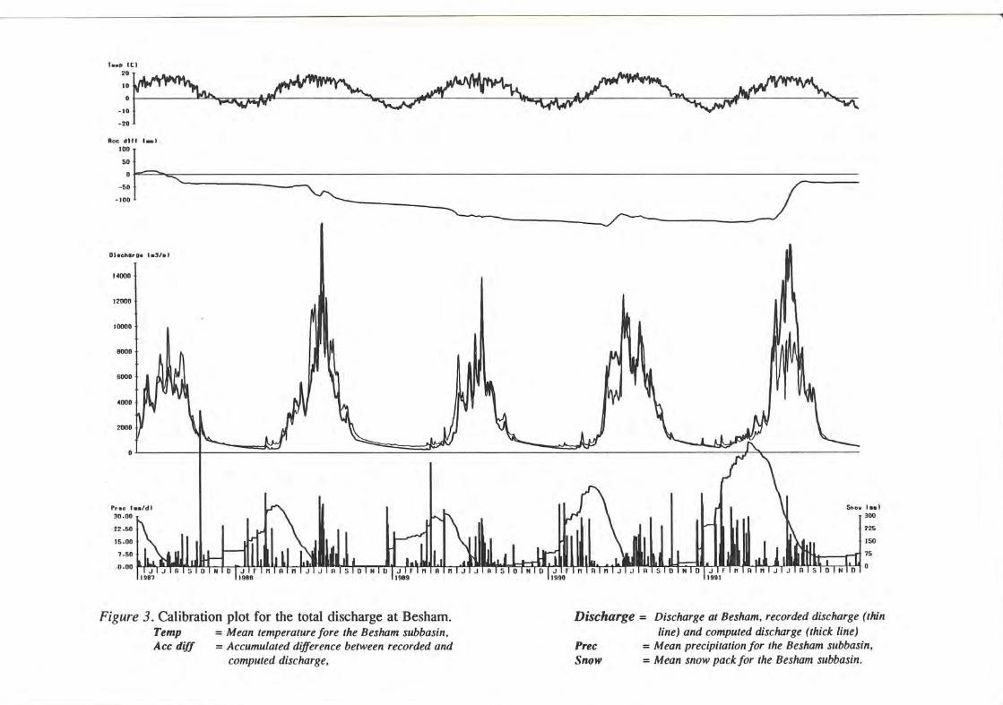
Figure 3. Calibration plot for the total discharge at Besham. Temp = Mean temperature fore the Besham subbasin, Acc di// = Accumulated difference between recorded and
computed discharge,
Snow la•l 300
225
150
15
D
Discharge = Discharge at Besham, recorded discharge (thin
Prec Snow
line) and computed discharge (thick line) = Mean precipitation for the Besham subbasin, = Mean snow pack for the Besham subbasin.
l••P It) 40
20
-20
ll\f lev l • 3/al
14000
12000
10000
Pr•o l••/d) 90-00
46-00
30 -00
16-00
o.oo
Figure 4. Calibration plot for the local inflow to the Tarbela reservoir. Temp = Mean temperature fore the Tarbela subbasin, Acc diff = Accumulated diff erence between recorded and
computed inflow
Snov laa) 800
460
300
ISO
0
lnflow = Total recorded injlow to the Tarbela dam (thin line) and computed local injlow (thick line) ,
Prec = Mean precipitation for the Tarbela subbasin, Snow = Mean snow packfor the Tarbela subbasin.
SMHI Reports Hydrology (RH)
1. Sten Bergström, Per Sanden and Marie Gardelin (1990) Analysis of climate-induced hydrochemical variations in till aquifers.
2. Maja Brandt (1990) Human impacts and weather-dependent effects on water balance and water quality in some Swedish river basins.
3. Joakim Harlin (1992) Hydrological modelling of extreme floods in Sweden.
4. Sten Bergström (1992) The HBV model - its structure and applications.
5. Per Sanden and Per Warfvinge (1992) Modelling groundwater response to acidification.
6. Göran Lindström (1993) Floods in Sweden - Trends and occurrence.
7. Sten Bergström and Bengt Carlsson (1993) Hydrology of the Baltic Basin. Inflow of fresh water from rivers and land for tbe period 1950 - 1990.
8. Barbro Johansson (1993) Modelling tbe effects of wetland drainage on high flows.
SMHI Hydrologi (H)
1. Bengt Carlsson (1985) Hydrokemiska data frän de svenska fältforskningsområdena.
2. Martin Hägg ström och Magnus Persson ( 1986) Utvärdering av 1985 ärs värflödesprognoser.
3. Sten Bergström, Ulf Ehlin, SMHI, och Per-Eric Ohlsson, V ASO ( 1986) Riktlinjer och praxis vid dimensionering av utskov och dammar i USA. Rapport frän en studieresa i oktober 1985.
4. Barbro Johansson, Erland Bergstrand och Torbjörn Jutman (1986) Skäneprojektet - Hydrologisk och oceanografisk information för vattenplanering - Ett pilotprojekt.
5. Martin Häggström (1986) översiktlig sammanställning av den geografiska fördelningen av skador främst pä dammar i samband med septemberflödet 1985.
6. Barbro Johansson (1986) Vattenföringsberllkningar i Södermanlands län - ett försöksprojekt.
7. Maja Brandt (1986) Areella snöstudier.
8. Bengt Carlsson, Sten Bergström, Maja Brandt och Göran Lindström (1987) PULS-modellen: Struktur och tillämpningar.
9. Lennart Funkquist (1987) Numerisk beräkning av vägor i kraftverksdammar.
10. Barbro Johansson, Magnus Persson, Enrique Aranibar and Robert Llobet (1987) Application of tbe HBV model to Bolivian basins.
11 . Cecilia Ambjörn, Enrique Aranibar and Roberto Llobet (1987) Montbly strearnflow simulation in Bolivian basins with a stochastic model.
12. Kurt Ehlert, Torbjörn Lindkvist och Todor Milanov (1987) De svenska huvudvattendragens namn och mynningspunkter.
13. Göran Lindström (1987) Analys av avrinningsserier för uppskattning av effektivt regn.
14. Maja Brandt, Sten Bergström, Marie Gardelin och Göran Lindström (1987) Modellberäkning av extrem effektiv nederbörd.
15. Håkan Danielsson och Torbjörn Lindkvist (1987) Sjökarte- och sjöuppgifter. Register 1987.
16. Martin Häggström och Magnus Persson (1987) Utvärdering av 1986 ärs värflödesprognoser.
17. Bertil Eriksson, Barbro Johansson, Katarina Losjö och Haldo Vedin (1987) Skogsskador - klimat.
18. Maja Brandt (1987) Bestämning av optimalt klimatstationsnät för hydrologiska prognoser.
19. Martin Häggström och Magnus Persson (1988) Utvärdering av 1987 ärs värflödesprognoser.
20. Todor Milanov (1988) Frysförluster av vatten.
21. Martin Häggströrn, Göran Lindström, Luz Amelia Sandoval and Maria Elvira Vega (1988) Application of tbe HBV rnodel to tbe upper Rfo Cauca basin.
L
22. Mats Mo berg och Maja Brandt ( 1988) Snökartläggning med satellitdata i Kultsjöns avrinningsområde.
23. Martin Gotthardsson och Sten Lindell (1989) Hydrologiskt stationsnät. Svenskt Vattenarkiv.
24. Martin Häggström, Göran Lindström, Luz Amelia Sandoval y Maria Elvira Vega (1989) Aplicacion del modelo HB V a la cuenca superior del Rfo Cauca.
25. Gun Zachrisson (1989) Svära islossningar i Torneälven. Förslag till skadeförebyggande åtgärder.
26. Martin Häggström (1989) Anpassning av HBV-modellen till Torneälven.
27. Martin Häggström and Göran Lindströril (1990) Application of the HBV model to six Centralamerican rivers.
28. Sten Bergström (1990) Parametervärden för HBV-modellen i Sverige. Erfarenheter frän modellkalibreringar under perioden 1975 - 1989.
29. Urban Svensson och Ingemar Holmström (1990) Spridningsstudier i Glan.
30. Torbjörn Jutman (1991) Analys av avrinningens trender i Sverige.
31. Mercedes Rodriguez, Barbro Johansson, Göran Lindström, Eduardo Pianos y Alfredo Remont (1991) Aplicacion del modelo HBV a la cuenca del Rfo Cauto en Cuba.
32. Erik Arner (1991) Simulering av värflöden med HBV-modellen.
33. Maja Brandt (1991) Snömätning med georadar och snötaxeringar i övre Luleälven.
34. Bent Göransson, Maja Brandt och Hans Bertil Wittgren (1991) Markläckage och vattendragstransport av kväve och fosfor i Roxen/Glan-systemet, Östergötland.
35. Ulf Ehlin och Per-Eric Oblsson, VASO (1991) Utbyggd hydrologisk prognos- och varningstjänst. Rapport frän studieresa i USA 1991-04-22--30.
36. Martin Gotthardsson, Pia Rystam och Sven-Erik Westman (1992) Hydrologiska stationsnät/Hydrological network. Svenskt Vattenarkiv.
37. Maja Brandt (1992) Skogens inverkan pä vattenbalansen.
38. Joakim Harlin, Göran Lindström, Mikael Sundby (SMHI) och Claes-Olof Brandesten (Vattenfall Hydropower AB) (1992) Känslighetsanalys av Flödeskommittens riktlinjer för dimensionering av bel älv.
39. Sten Lindell (1993) Realtidsbestämning av arealnederbörd.
40. Vattenföring i Sverige. Del 1. Vattendrag till Bottenviken (under utgivning). Svenskt Vattenarkiv.
41. Vattenföring i Sverige. Del 2. Vattendrag till Bottenhavet. (under utgivning). Svenskt vattenarkiv
42. Vattenföring i Sverige. Del 3. Vattendrag till Egentliga Östersjön. (1993) Svenskt Vattenarkiv.
43. Vattenföring i Sverige. Del 4. Vattendrag till Västerhavet (under utgivning). Svenskt Vattenarkiv.
44. Martin Häggström och Jörgen Sahlberg (1993) Analys av snösmältningsförlopp.
45. Magnus Persson (1993) Utnyttjande av temperaturens persistens vid beräkning av volymsprognoser med HBV-modellen.
46. Göran Lindström, Joakim Harlin och Judith Olofsson (1993) Uppföljning av Flödeskommittens riktlinjer.
47. Bengt Carlsson (1993) Alkalinitets- och pH-förändringar i Umeälven orsakade av minimitappning.
48. Häkan Sanner, Joakim Harlin and Magnus Persson (1994) Application of the HBV model to the Upper Indus River for inflow forecasting to the Tarbela dam.
!) I I
\) I
SMHI Swedish meteorological and hydrological institute
S-60176 Norrköping, Sweden. Tel. +4611158000. Telex 64400 smhi s.