SN No. 576E Project: Cold Trap CFD Modeling Page …Fundamentals of Heat and Mass Transfer, 4th...

SN No. 576E Project: Cold Trap CFD Modeling Page 1 David B. Walter – ------------------------------------------------------------------------------------------------------------ 3/6/2003 – Task Title: Cold Trap CFD Modeling for TEF KTI (20.06002.01.091) Investigators:

Randy Fedors Steve Green Frank Dodge Steve Svedemann David Walter

Computers and Software: CFD modeling and other miscellaneous computer tasks (data analysis, word processing, etc.) were performed with one of two identical Dell OptiPlex PCs with Intel Pentium 4 processors and Windows 2000 operating system. System information reports for the two computers used are contained in Walter-PC.txt and Hatton-PC.txt. The following software was used: Software Name and Version Description Associated File

Extension Microsoft Word 2000 (9.0 4402 SR-1)

Word Processing *.doc

Microsoft Excel 2000 (9.0 4402 SR-1)

Spreadsheet *.xls

AutoCAD Light 2000 General CAD *.dwg MathCAD 2000 Professional Engineering Calculations *.mcd Flow-3D Ver. 8.1.1 Computational Fluid Dynamics various Objective: The primary goal of the numeric modeling was to demonstrate that natural convection in the drift can transport moisture from the hot end to the cold end of the drift. As a secondary goal, the modeling of the laboratory scale cold trap experiment was used to refine and verify the modeling techniques for use in larger scale modeling by comparing the numerical and experimental results. --------------------------------------------------------------------------------------------------------------------- 3/6/2003 – Description of approach: Numerical modeling of the cold trap was accomplished through the use of a commercially available finite volume computational fluid dynamics (CFD) code called FLOW-3D® from Flow Science, Inc. (683 Harkle Road, Suite A, Santa Fe, NM 87505). Due to product updates, several versions of the code have been utilized during this analysis. The most recent upgrade that has been used for the last month is version 8.1.1. The code was installed with the Compaq Visual Fortran compiled version of the code. Quality assurance checks of this version and installation still need to be performed. The modeling results generated with previous revisions to the code can be considered preliminary; only the results obtained with the latest version will be reported. Therefore, only the last version of the code needs have to QA verification. The three-dimensional CFD model included the major components and geometry of the laboratory-scale cold trap experiment setup. A schematic based on measurements from

SN No. 576E Project: Cold Trap CFD Modeling Page 2 David B. Walter – ------------------------------------------------------------------------------------------------------------ Randy Fedors of the coldtrap assembly is shown in desktop_dimen-1.pdf. The schematic also lists some of the materials used in the model and the initial thermal conductivities used in the modeling effort. Some of these properties were calibrated during the CFD modeling process to more closely match the CFD results to the experimental test data. Another detailed schematic drawing of the CFD model geometry, solid material properties, boundary conditions, and other modeling parameters is shown in Coldtrap Model(1).pdf and Coldtrap Model(2).pdf. These schematics also show the CFD coordinate system, the actual CFD geometry, the thermal conductivities, and interface conductance values used in the final CFD simulations. The input files that will be referenced in subsequent entries will document any remaining physical and modeling parameters not shown in these schematics. To reduce the CFD simulation time, only half the cold trap geometry was modeled by imposing a symmetry condition in the x-z plane (vertical plane down the center of axis of the drift). The Boussinesq approximation was used to simulate the natural convection in the drift. That is, the air is assumed to be nominally incompressible in which the density varies with temperature but does not vary with pressure. FLOW-3D® does not have capabilities to readily model the evaporation and condensation processes that are present in the experiment or full-scale drift. In order to evaluate these key processes, the CFD model was used to determine the flow and temperature distributions in the drift assuming that the gas in the drift is composed of dry air. The moisture transport was then estimated from the CFD predictions as described in Steve Green’ scientific notebook (#536E). To summarize, the key assumptions of this analysis approach are: 1) properties of moist air are not significantly different than those of dry air, 2) the latent heat for the evaporation and condensation processes are negligible compared to heat transfer associated with conduction and convection in the model, 3) the diffusion rate of the water vapor in the a drift is adequate to keep the air throughout the drift completely saturated, and 4) the condensation and evaporation processes are always at equilibrium. --------------------------------------------------------------------------------------------------------------------- 3/22/2003 – Description of approach continued: The properties used for the air inside the drift are as follows: Dry Air Properties @ 325 K and 1 atm

Value Source

Specific Heat – Constant Volume (Cv)

770 J/kg/K * Moran and Shapiro. Fundamentals of Engineering Thermodynamics, 2nd Edition. John Wiley and Sons, Inc., New York 1992.

Density (ρ) 1.08 kg/m3 Incropera and DeWitt. Fundamentals of Heat and Mass Transfer, 4th Edition. John Wiley and Sons, Inc., New York 1996.

SN No. 576E Project: Cold Trap CFD Modeling Page 3 David B. Walter – ------------------------------------------------------------------------------------------------------------ Thermal Conductivity (k)

0.028 W/m/K Incropera and DeWitt. Fundamentals of Heat and Mass Transfer, 4th Edition. John Wiley and Sons, Inc., New York 1996.

Thermal Expansion Coefficient

3.33E-03 kg/m3/K Incropera and DeWitt. Fundamentals of Heat and Mass Transfer, 4th Edition. John Wiley and Sons, Inc., New York 1996.

Dynamic Viscosity (μ) 1.85E-05 kg/m/s Incropera and DeWitt. Fundamentals of Heat and Mass Transfer, 4th Edition. John Wiley and Sons, Inc., New York 1996.

*Noticed that this value may be too high (should be around 720 for air at 325, may have been adjusted for moist air [?]). These property values are for dry air at 325 K and 1 atmosphere. We’ve made an assumption that these property values will not be significantly different for moist air. The intent of the CFD model was to simulate the coldtrap experiment to evaluate the air transport and temperature distribution inside the drift. The goal is to 1) demonstrate the moisture transport phenomena that is thought to be caused by natural convection due to a cold wall and hot surfaces (waste package) in the drift and 2) verify the modeling fidelity by matching as closely as possible the temperature measurements taken in the desktop (~1:100 scale) experiment. --------------------------------------------------------------------------------------------------------------------- 4/3/2003 – The modeling effort described in this notebook describes the simulation effort from mid-February to present. Modeling conducted from October to February can be considered preliminary and therefore does not require detailed discussion in this scientific notebook. The modeling effort focused on simulating the conditions of the laboratory experiment. This allowed many of the modeling parameters (solid material conductivity, interface conductance values, and convection coefficient values) to be modified (calibrated) to more closely match the experimental results. The table below summarizes the simulations that were conducted, the experimental tests that the CFD results were compared to, and associated input files for the simulations. Simulation Description Input Filename Test Comparison Dry Test 3.37 Watts prepinr.Coldtrap4 Tests 16d Wet Test 3.37 Watts prepinr.wet_3w Tests 11 & 14 Wet Test 1.25 Watts prepinr.wet_1w Tests 11 & 14 Wet Test 5.25 Watts prepinr.wet_5w Tests 11 & 14 During the preliminary modeling effort, we discovered that the initial values that we used for the saturated sand thermal conductivity (~0.24 W/m/K) was not providing a good match with the test results with saturated sand. In particular, the CFD was predicting temperature gradients in the sand of approximately 10 times that of the test results. With the assumption that we were modeling the same amount of heat flux as was present in the experiment, led us to suspect the value that we were using for the sand thermal conductivity. We suspected that there might be a convection effect in the sand

SN No. 576E Project: Cold Trap CFD Modeling Page 4 David B. Walter – ------------------------------------------------------------------------------------------------------------ that may effectively raise the thermal conductivity when the sand was saturated. To investigate this hypothesis, we elected to conduct some testing and modeling with dry sand. The initial modeling effort focused on trying to match the test results from the 3.37 watt dry test (Test 16d) with the CFD results. This effort included refining the model mesh, experimenting with different convection coefficients, adjusting the thermal conductivity and interface conductance values of the heater stand off, and adjusting the thermal conductivity of the dry sand. This effort included many different simulations restarts with modified modeling parameters to achieve the closest match to the experimental results. The prepinr.Coldtrap4 is the final input file used for the dry run simulation. The comments section at the beginning of the file contains dated entries that explain the changes made in each modeling iteration. Dry3.xls contains all the important mesh dependent output data (obstacle temperatures, air temperatures, x-velocities for air) for this dry simulation. Dry3-comparison.xls contains more information regarding the comparison to the laboratory experimental results. The key modeling parameters for this dry test simulation were as follows:

Dry sand thermal conductivity = 0.22 W/m/K Ceramic Heater Stand Off Modeling

o Thermal Conductivity = 6.8 W/m/K o Thermal Interface Conductance = 113 W/m2/K (equivalent to conduction

through .01” air gap) – this interface conductance was used for interface between the heater and the stand off and the stand off and the ceramic drift tube.

Convection coefficients were not specified (FLOW-3D was allowed to estimate the convection coefficients)

Figures 4/3/03-1 and 4/3/03-2 compare the CFD results with the measured air and solid temperatures for the dry test conducted at 3.37 watts (Test 16d). At the heater (Figure 11/13/03-4/3/03-1) the air temperature is significantly hotter in the CFD results than the measured results. The solid temperatures above the heater do match fairly well, with the CFD results approximately 1.5°C below the measured temperatures. The same trend regarding the difference between the solid temperatures above and below the heater, that was observed with the wet tests, is also present with this dry test data. The measured data indicates that the solid material below the heater is hotter than the material above the heater. The CFD results show the opposite trend with the material below the heater cooler than the material above the heater. The data at x=.165m (Figure 4/3/03-2) shows a good comparison between both the air temperature and the solid temperatures above the drift. One interesting observation is that the CFD air temperature at this location is slightly lower than the measured air temperature. Recall that at the heater (Figure 4/3/03-1), the CFD air temperature was ~20°C hotter than the measured results.

SN No. 576E Project: Cold Trap CFD Modeling Page 5 David B. Walter – ------------------------------------------------------------------------------------------------------------

Comparison of CFD vs. Test Results(Dry Test)

Heater Power = 3.37 watts x-location = 0.267 m

20.0

30.0

40.0

50.0

60.0

70.0

80.0

90.0

-0.2 -0.15 -0.1 -0.05 0 0.05 0.1 0.15 0.2

Vertical Height from Center of Drift (m)

Tem

pera

ture

(°C

)

Test 16d CFD - Solid Temp. CFD - Fluid Temp. OD of Drift Tube Lexan Walls

Figure 4/3/03-1. Comparison of the CFD and measured temperatures of Test 16d at x=0.267 (~ center of heater). The CFD results for the air temperature above the heater was more than 20°C hotter than the measured temperature. [Source: Dry3-comparison.xls]


Comparison of CFD vs. Test Results(Dry Test)


20.0

25.0

30.0

35.0

40.0

45.0

50.0

0 0.02 0.04 0.06 0.08 0.1 0.12 0.14 0.16 0.18 0.2


Tem

pera

ture

(°C

)

Test 16d CFD - Solid Temp. CFD - Fluid Temp. OD of Drift Tube Lexan Walls

Figure 4/3/03-2. Comparison of the CFD and measured temperatures of Test 16d at x=0.165 midway between heater and the mid-plane of the drift). The CFD results for the air temperature were ~1.5°C lower than the measured air temperature at this location. The temperatures in the sand, lexan, and insulation show good comparison. [Source: Dry3-comparison.xls]

-------------------------------------------------------------------------------------------------------------------- 4/4/2003 – The next step in the modeling process was to change the thermal conductivity of the sand to simulate the wet tests with saturated sand at 3.37 watts. Using the wet test data (Test 11) the thermal conductivity of the thermal conductivity of the sand was estimated at 8 times that of the dry test or 1.76 W/m/K. With this value, the temperature gradient in the model matched fairly closely with the experimental results for the sand above the heater, therefore no adjustment was necessary. No other modeling parameters were modified. The prepinr.Wet3 is the final input file used for the wet run simulation at 3.37 watts. The comments section at the beginning of the file contains dated entries that explain the changes made in each modeling iteration. Wet3.xls contains all the important mesh dependent output data (obstacle temperatures, air temperatures, x-velocities for air) as well as a comparison to the results of Tests 11 and 14.

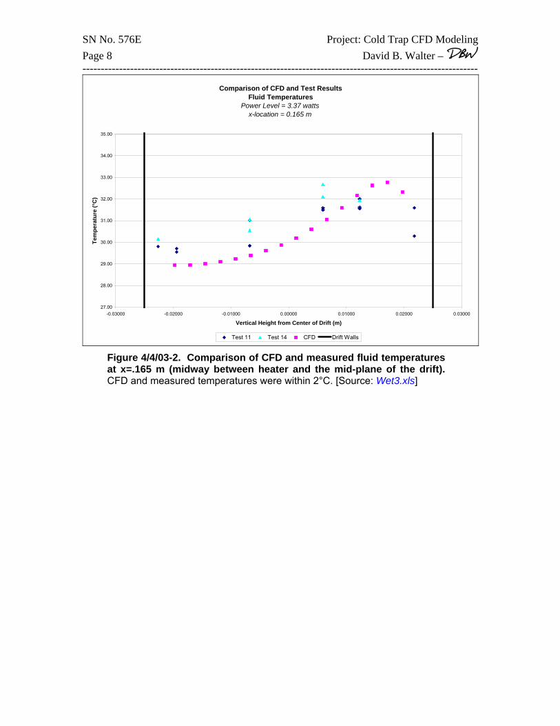
SN No. 576E Project: Cold Trap CFD Modeling Page 7 David B. Walter – ------------------------------------------------------------------------------------------------------------ Figures 4/4/03-1, 4/4/03-2, and 4/4/03-3 show comparisons of the CFD and measured fluid temperatures at different locations along the drift for Tests 11 and 14 (wet tests). The data at x=.279m (Figure 4/4/03-1) shows the largest discrepancy between the measured data and the CFD results. The fluid temperatures at this location are approximately 45°C hotter than the measurements. The data at x=.165 m (Figure 4/4/03-2) show somewhat better results with the CFD temperatures deviating by approximately ±2°C from the measurements. The temperature gradient for the CFD results show the same trend, with the hotter fluid at the top of the drift. The magnitudes of the gradient are slightly different though, with the CFD results showing a distribution ranging from approximately 29 to 32.8°C and the measured results ranging from approximately 29.6 to 31.8°C. The data at x=.063 (Figure 4/4/03-3) shows a decent match (less than 0.5°C difference) between the CFD results and the results of Test 11. An additional observation is that there appears to be a slight temperature discrepancy between Test 11 and 14 at this location in the drift.

Comparison of CFD and Test ResultsFluid Temperatures

Power Level = 3.37 wattsx-location = 0.279 m

25.00

35.00

45.00

55.00

65.00

75.00

85.00

95.00

-0.03000 -0.02000 -0.01000 0.00000 0.01000 0.02000 0.03000


Tem

pera

ture

(°C

)

Test 11 Test 14 CFD Drift Walls

Figure 4/4/03-1. Comparison of CFD and measure fluid temperatures at x=0.279 m (~ center of heater). CFD temperatures were approximately 45°C hotter than the measured temperatures. [Source: Wet3.xls]




27.00

28.00

29.00

30.00

31.00

32.00

33.00

34.00

35.00

-0.03000 -0.02000 -0.01000 0.00000 0.01000 0.02000 0.03000


Tem

pera

ture

(°C

)


Figure 4/4/03-2. Comparison of CFD and measured fluid temperatures at x=.165 m (midway between heater and the mid-plane of the drift). CFD and measured temperatures were within 2°C. [Source: Wet3.xls]




27.00

27.50

28.00

28.50

29.00

29.50

30.00

-0.03000 -0.02000 -0.01000 0.00000 0.01000 0.02000 0.03000


Tem

pera

ture

(°C

)


Figure 4/4/03-3. Comparison of CFD and measured fluid temperatures at x=.063 (near mid-plane of drift). CFD results are within 0.5°C of the measured results for Test 11 and show a similar temperature distribution trend. The measured temperatures for Test 14 do not match the measured temperatures for Test 11 or the CFD results. [Source: Wet3.xls]

Figures 4/4/03-4 and 4/4/03-5 show comparisons of the CFD results and the measured temperatures in the solid materials (drift tube, sand, lexan, and insulation) of Tests 11 and 14 (wet tests). The data in Figure 4/4/03-4 compares the temperatures in the sand above and below the heater and shows that the CFD results are 2 to 7°C lower than the measurements for Tests 11 and 14. One observation regarding this data is that, for both test 11 and 14, the temperatures in the sand below the heater were higher than the temperatures in the sand above the heater. The CFD results showed the opposite trend – the temperatures below the heater were lower than those above. Another discrepancy to note is the temperature gradient in the sand. The gradient appears to match fairly closely for the sand above the heater, but the below the heater, the measured gradient is much higher than the CFD results show. A final observation is that, like in Figure 4/4/03-3, there is temperature discrepancy between the results for Tests 11 and 14 for the solid material temperatures at this location. The data at x=.165 m (Figure 4/4/03-5) shows similar results to those shown in Figure 4/4/03-4. The CFD results matched fairly closely with measurements for Test 11 for the thermocouples above the drift. At this location there is no substantial difference in the gradients above or below the drift between the CFD and measured results. A final observation is that discrepancy between the temperatures of Test 11 and 14 are also present at this location in the drift.


Comparison of CFD and Test ResultsSolid Temperatures


27.00

29.00

31.00

33.00

35.00

37.00

39.00

41.00

-0.20000 -0.15000 -0.10000 -0.05000 0.00000 0.05000 0.10000 0.15000 0.200


Tem

pera

ture

(°C

)

Test 11 Test 14 CFD Drift Tube/Sand Interface Sand/Lexan Interface Figure 4/4/03-4. Comparison of the measured and CFD temperatures in the solid materials of the model. Data shown is at x=.267 m (~ heater mid-point). CFD results matched closely with the temperatures in the sand above the heater for Test 11. Below the heater, the test measurements show a steeper temperature gradient and higher overall temperature than the CFD results. [Source: Wet3.xls]


Comparison of CFD and Test ResultsSolid Temperatures


27.00

28.00

29.00

30.00

31.00

32.00

33.00

-0.20000 -0.15000 -0.10000 -0.05000 0.00000 0.05000 0.10000 0.15000 0.20000


Tem

pera

ture

(°C

)

Test 11 Test 14 CFD Drift Tube/Sand Interface Sand/Lexan Interface

Figure 4/4/03-5. Comparison of the measured and CFD temperatures in the solid materials of the model. Data shown is at x=.165 m (~ heater mid-point). CFD results matched closely with the temperatures in the sand above the heater for Test 11. [Source: Wet3.xls]

After the completion of the 3.37 watt simulation, additional simulations were conducted at different experimental test power levels (1.25 watts and 5.25 watts). Only the heater input power was changed for these simulations; no other modeling parameters were changed. The input files for these simulations were prepinr.Wet1 and prepinr.Wet5. The results are shown in Wet1.xls and Wet5.xls. -------------------------------------------------------------------------------------------------------------------- 4/4/2003 After the completion of the simulations, the post-processing calculations (as described in the 3/3/2003 entry) were performed to estimate the vapor transport in the wet test simulations. The results and calculation for the 3.37-watt simulation are contained in Wet3.xls. The results and calculations for the 1.25-watt simulation are shown in Wet1.xls. The post-processing analysis of the 5.25-watt simulation have not been completed.

SN No. 576E Project: Cold Trap CFD Modeling Page 12 David B. Walter – ------------------------------------------------------------------------------------------------------------ Figure 4/4/03-6 shows temperature and x-velocity contour plots with the y-z flow velocity vectors of the fluid at one of the cross-sections along the drift. This figure allows for a further explanation of the post-processing technique that is used to estimate the vapor transport along the drift.

Figure 4/4/03-6. Contour and vector plots of the CFD results with a heater power of 3.37 watts for a drift cross-section at x=0.202 m. The left plot shows the temperature contour; the right plot shows the x-velocity (along the axis of the drift) contour. Both plots show the y-z velocity vectors of the fluid flow. X-Velocity values that are negative indicate that flow is moving from the heater end to the cold end of the drift. The plots show that the natural convection in the drift causes hot air to move toward the cold end at the top of the drift, while colder air moves back toward the heater at the bottom of the drift. (Units: temperature – K, velocity – m/s) [Source: prepinr.wet_3w]

As described previously, the results obtained from the CFD represent dry air in the drift. The vapor transport is estimated by first extracting from the CFD results the temperature, x-velocity, and y-z area of each cell in the drift at a particular cross-section. The cell fluid temperature is used to estimate the mass of water in each cell with the assumption that the air is at saturated conditions. Combining this information with the x-velocity and area of each cell (using the calculations shown previously) provides an estimate of the water transport rate for each cell. The water transport for all the cells at each cross-section along the drift are then added to provide the total vapor transport in the drift. The contour plots in Figure 4/4/03-6 show the key information that is used for this post-processing analysis. Because of the natural convection in the drift, the warmer air at the top of the drift moves from the heater end to the cold end of the drift; the cooler fluid moves along the bottom of the drift back toward the heater. At saturated conditions, the warmer air holds more water and therefore transports more water away from the heater than the cooler air transports back to the heater. As a result, the net transport rate is such that moisture moves down the drift away from the heater. Recall that in the CFD

SN No. 576E Project: Cold Trap CFD Modeling Page 13 David B. Walter – ------------------------------------------------------------------------------------------------------------ coordinate system the positive x-direction is axially along the drift from the cold end to the hot end, so this net flow rate, away from the heater, has a negative magnitude. The results of these calculations for each cross-section along the drift are shown in Figure 4/4/03-7. The plot shows the net vapor flow rate and the negative component of the air flow rate that is flowing along the drift. Only the negative component of the air flow rate is shown because the net air flow rate is zero due to conservation of mass. The analysis shows that the vapor transport rate decays to zero near the mid-point of the drift (x=0). The air flow rate decays in a similar manner, but it continues to flow down to the end of the drift at the cold wall. The reason that the net vapor rate does not continue with the air flow rate past the midpoint of the drift is because there is no temperature differential between the positive and negative air flow at these cross-sections. In other words, the air flowing in the negative direction (away from the heater end) is transporting the same amount of vapor as the air flowing in the positive direction (toward the heater).

Vapor and Air Mass Flow Rate Along DriftHeater Power = 3.37 watts

-20

-15

-10

-5

0

5

10

15

20

-0.4 -0.3 -0.2 -0.1 0 0.1 0.2 0.3 0.4

Distance Along Axis of the Drift (m)

Net

Vap

or M

ass

Tran

spor

t (g-

wat

er/h

r)

-100

-75

-50

-25

0

25

50

75

100

Neg

ativ

e C

ompo

nent

of A

ir M

ass

Flow

Rat

e (g

/hr)

Vapor Flow Rate Air Flow Rate

Location of Heater

Figure 4/4/03-7. Plot showing numerical analysis results of the flow rate at which vapor and air are transported along the drift due to natural convection. The case shown is with a heater power of 3.37 watts. Negative flow rate values indicate that fluid is being transported from the heater end to the cold end of the drift. The transport of vapor decays to approximately zero at the drift mid-plane (x=0). [Source: wet3.xls]

One other interesting note about Figure 4/4/03-7 is the disturbance in both the air flow and vapor flow at the heater. This is due to the thermal plume caused by the convection at the heater surface. Figure 4/4/03-8 shows a temperature contour plot of the fluid

SN No. 576E Project: Cold Trap CFD Modeling Page 14 David B. Walter – ------------------------------------------------------------------------------------------------------------ around the heater in the x-z plane at the drift centerline. The velocity vectors to the left of the plume (from x=.260 to .280 m) and close to heater surface show a positive x component. This fluid is hotter than the fluid at the top of the drift, which has a negative x-component of the velocity vector. Therefore, the calculated net vapor transport rate is positive, which explains the positive values shown around the heater in Figure 4/4/03-7. These results are misleading though because the assumption that the fluid is at saturated conditions is most likely not valid in this region near the heater. In this region, the air is heated quickly, and it is suspect whether enough water will be present and the diffusion rate will be adequate the keep the air at saturated conditions. Most likely the air will be well under the saturation point, making the analysis technique invalid in this region. However, this should not affect the estimated transport rate calculations in the remaining portions of the drift, since it is reasonable to assume that, in these regions, the air will be saturated and at equilibrium.

Figure 4/4/03-8. Temperature contour and velocity vector plot of the CFD results in the center of the drift near the heater. The case shown is with a heater power of 3.37 watts. The temperature contour shows a distinctive thermal plume rising from the heater surface. (Units: temperature – K, velocity – m/s). [Source: prepinr.wet_3w]

After the analysis, I attempted to verify one of the key assumptions for this analysis: the latent heat for the evaporation and condensation processes are negligible compared to heat transfer associated with conduction and convection in the model (see 3/6/2003 entry). I calculated the latent heat required to turn free water at the saturation

SN No. 576E Project: Cold Trap CFD Modeling Page 15 David B. Walter – ------------------------------------------------------------------------------------------------------------ temperature to vapor at the transport rates predicted in this analysis. The results are for the 1.25-watt and 5.25 watt cases are present below.

Simulation Vapor Rate @ x=.25m (g/hr)

Heat of Vaporization @ 50° C* (J/g)

Calculate Latent Heat Rate

(Watts) 3.37-watt Simulation

5.96 2382.7 3.9

1.25-watt Simulation

1.94 2382.7 1.28

*From Moran and Shapiro (See citation in 3/22/2003 entry) Obviously since the latent heat required is more than the total heater power, this assumption is not valid. In reality since latent heat is significant, the temperatures and flow rates around the heater will be much lower than the predicted values. That fact that this assumption was invalid limits that magnitude of the predicted transport rate, but does not invalidate the overall conclusion that natural convection will transport moisture along the drift. Conclusion: future cold-trap modeling should attempt to simulate this evaporation/condensation process. -------------------------------------------------------------------------------------------------------------------- 4/7/2003 Overall observations regarding CFD results: • The CFD air temperatures at the heater are significantly hotter than the measured results for both the wet and dry tests (see Figures 4/3/03-1 and 4/4/03-1). At locations further down the drift (away from the heater) the overall air temperatures match fairly closely with the measured temperatures (see Figures 4/4/03-2, 4/4/03-3, and 4/3/03-2). Therefore, the temperature gradient of the air along the drift is significantly higher for the CFD prediction than for the measured results. • The CFD air temperatures at the two locations away from the heater for the wet tests (see Figures 4/4/03-2 and 4/4/03-3) show the same basic trend with the hotter fluid at the top of the drift and the cooler fluid at the bottom of the drift. • The temperatures in the solid materials matched fairly well for both the wet and dry tests (See Figures 4/4/03-4, 4/4/03-5, 4/4/03-6, and 4/4/03-7). The most notable discrepancy was the fact that the measured solid temperatures directly below the heater were hotter than those in the solid material above the drift, while the CFD results showed the opposite trend with the solid material below the heater cooler than the material above. • There is a temperature discrepancy between results for Test 11 and 14 (see Figures 4/4/03-3, 4/4/03-4, and 4/4/03-5). Noting that the temperatures increased significantly for the dry test, it may be reasonable to assume that the discrepancy between Test 11 and 14 may be a result of slightly different water saturations in the sand.

Possible causes for differences between the CFD and measured results:

SN No. 576E Project: Cold Trap CFD Modeling Page 16 David B. Walter – ------------------------------------------------------------------------------------------------------------ • Latent heat of vaporization assumption: For the wet tests, the lack of latent heat in the model helps explain the reason that the predicted air temperatures above the heater were so much greater than the measured values. This also may explain the higher predicted temperature gradient in the fluid along the drift. The heat transported along with the moisture in the drift will cause the temperatures away from the heater to be higher, lowering the temperature gradient. This latent heat affect does not explain, however, why the predicted temperatures in the dry test (with no latent heat) were so much hotter above the heater than the measured results.

• Boundary Conditions: The boundary conditions in the CFD model were set at a constant temperature of 300K (26.8°C) for all six sides including the cold plate. The tests were conducted with a cold plate temperature of 20°C. Also, the bottom of the experimental apparatus was set on a piece of Styrofoam insulation on a table in the lab. The extra insulation on the bottom of the experiment may account for the greater measured temperatures in the sand below the heater. The differences in the cold wall temperatures may partially account for higher predicted air temperatures at the heater, but it does not explain why the air temperature gradient in the fluid along the drift is higher in the CFD model.

• Thermal conductivity of the solid materials: Accurate thermal conductivities for many of the materials in the model were difficult to obtain. In particular, the text book values for dry sand and calculated values for saturated sand did not adequately match the thermal gradients in the CFD model. The values for both dry and wet sand used in the CFD model were calibrated to more closely match the CFD results. The calibrated wet sand conductivity value was on the order of ten times greater than the value originally calculated. One possible cause for this discrepancy was that thermal buoyancy in the water was creating a convection effect that significantly raised the effective thermal conductivity. This effect was modeled by simply raising the thermal conductivity of the sand throughout the model. In reality, the sand below the heater, with the heat being conducted from above, would not see this effect because it is thermally stable. If this hypothesis is true, the sand below heater should have a lower effective conductivity than sand above the drift. This may explain why the predicted temperatures below the heater were lower than the predicted temperatures above the heater.

• Heater stand: In the experimental apparatus, the heater was held up off the bottom of the drift with a small piece ceramic tube. The ceramic tube had a outside diameter smaller than the inside diameter of the drift and an inside diameter larger than the outside diameter of the heater. This geometry created line contacts and small air volumes that were difficult to model with the mesh resolution. The geometry was modeled with a solid material that was mated to both the heater and the drift wall. The line contacts were modeled with interface conductance parameters. It was difficult to estimate what value to use for these convection coefficients. This imprecise modeling of the heater stand has an effect on the predicted amount heat that is conducted from the heater to directly the bottom of the drift tube. This may account for some of the discrepancies of the solid temperatures below the heater. It is difficult to determine the exact cause of the discrepancies between the model and measured results. Further analysis would have to be conducted with a less complex model with better-known material properties to properly develop and refine this CFD modeling technique. The results do show that the CFD model does properly model the basic temperature trends in the model and should provide reasonable assessment of the cold trap vapor transport process.

SN No. 576E Project: Cold Trap CFD Modeling Page 17 David B. Walter – ------------------------------------------------------------------------------------------------------------ -------------------------------------------------------------------------------------------------------------------- 4/7/2003 An installation test was conducted on FLOW-3D version 8.1.1 on 4/2/03. A memo (FLOW-3D_Validation040303.pdf) documenting the results of the tests was sent to Bruce Mabrito on 4/7/03. -------------------------------------------------------------------------------------------------------------------- 4/7/2003 During the model development, we were trying to find an explanation for the air temperature above the heater being so much hotter than the experimental results. One possibility that we investigated was radiation from the heater to the drift walls. The thought was that in the experiment, heat was being radiated directly to the drift walls without heating the air. The following calculations were performed in a MathCAD sheet (radiation.mcd) to investigate this theory.

q12 σ A1, T1, T2, ε1, ε2, r1, r2,( ) 0.181W=

Solution:

Emissivity numbers from Mark's Handbook - 9th, Table 4.3.2

emissivity of alumina (.6 to .33 @ 260 - 680 °C)ε2 .6:=

emissivity of 316 SS (.57 to .66 @ 230 - 870 °C)ε1 .57:=

Temperatures from dry test 16bT2 37 273.15+( )K:=T1 86 273.15+( )K:=

A1 7.854 10 4−× m2=A1 2π r1⋅ l⋅:=

l .05m:=r2 .025m:=r1 .0025m:=

Stefan-Boltzmann Constantσ 5.670 10 8−⋅W

m2 K4⋅:=

Knowns:

Concentric long cylinders(Incropera and DeWitt, 4th ed - equation 13.25)

q12 σ A1, T1, T2, ε1, ε2, r1, r2,( )σ A1⋅ T1

4 T24−( )⋅

1ε1

1 ε2−

ε2

r1

r2⋅+

:=

Governing Equation:

Assumptions:1. Geometry is long concentric cylinders2. Uniform surface temperatures3. Neglect radiation to right drift wall (flat)4. Surfaces are diffuse and gray5. Space between surfaces is evacuated

Problem: Estimate the amount of heat that is radiated to the drift walls from the heater package.

SN No. 576E Project: Cold Trap CFD Modeling Page 18 David B. Walter – ------------------------------------------------------------------------------------------------------------ Conclusion: the radiated heat was only ~5% of the total heater power for this analyzed case at 3.37 watts. This is not enough to explain the significant differences between the air temperatures of the CFD and experimental results. Therefore, radiation is not a significant factor. =================================================================== Entries made into Scientific Notebook #576E for the period October 2002, to April 7, 2003, have been made by David Walter (April 7, 2003). No original text or figures entered into this Scientific Notebook has been removed 04/07/2003 ==================================================================

SN No. 576E Project: Cold Trap CFD Modeling Page 19 David B. Walter – ------------------------------------------------------------------------------------------------------------ 4/25/2003 Installed MathCad version 11.a on my computer. Information about Mathcad is available from www.Mathsoft.com. -------------------------------------------------------------------------------------------------------------------- 4/25/2003 Randy Fedors called yesterday to ask how we verified our assumption that the flow in the drift was laminar. The following Mathcad sheet (laminar.mcd) documents my calculations.

Flow is laminar

Conclusion:

Re mass Dh A P,( ), μ, A,( ) 36.09=

Solution:

Air at 1 atm and 325 K (Incropera and Dewitt. Fundamentals of Heat and Mass Transfer)

μ 196.4 10 7−⋅N s⋅

m2:=

Dh A P,( ) 0.031m=

Pπ d⋅2

d+:=

half of drift cross-sectionA12

π

4d2⋅⎛⎜

⎝⎞⎟⎠

:=

diameter of driftd .05m:=

Hydraulic Diameter Estimate

mass flow rate at exit of heater cross-section for wet CFD results at 3 watts(see wet3.xls)

mass 82gmhr

:=

Knowns:

Hydraulic DiameterDh A P,( )4 A⋅P

:=

Reynolds NumberRe mass Dh, μ, Acs,( )mass Dh⋅

μ Acs⋅:=

Governing Equation:

Assumptions: 1) Hydraulic diameter is based on half of drift diameter (half or flow is moving in one direction - half is moving the other direction)2) Reynolds numbers less than 2000 are laminar3) Reynolds number is highest at the heater4) Reynolds number is calculated based on bulk fluid flow down the drift5) Fluid properties are dry air

Problem: Determine if natural convection flow in coldtrap desktop experiment is laminar or turbulent

SN No. 576E Project: Cold Trap CFD Modeling Page 20 David B. Walter – ------------------------------------------------------------------------------------------------------------ -------------------------------------------------------------------------------------------------------------------- 8/9/2003 I’ve been working with the bench top (~1:100 scale) model in preparation for the sensitivity study that will be the topic for the SME paper in February. My recent goal has been to refine the model to so that it can be executed in shorter amount of time (<1 day preferable). The model used in the previous work took on the order to 1 week of calculation time to reach steady state conditions. Also, I wanted to complete a more throrough mesh dependency analysis before I begin the sensitivity analysis. After working to refine the model for a few weeks, I discovered that the heater input power specified in the model was for the full heater power (3.37 watts) rather than ½ the power because only half of the geometry was modeled. I reduced the heater power to 1.685 watts (3.37/2) and ran the model for the dry sand test. This model had a different mesh and numerical options than the previous model (see SN No. 576E entry 4/3/2003) but the geometry and fluid and material properties were left the same. The boundary temperatures were revised slightly. The input file for this revised model was prepin.Coldtrap-baseline6. The results of this model and the comparison to the Test 16d results are shown in the following three figures.

Comparison of CFD (baseline6r0) vs. Test Results (cttest16d)(Dry Test)


20.0

30.0

40.0

50.0

60.0

70.0

80.0

90.0

-0.2 -0.15 -0.1 -0.05 0 0.05 0.1 0.15 0.2


Tem

pera

ture

(°C

)

Test 16d CFD Temp OD of Drift Tube Lexan Walls

Figure 8/9/03-1. Comparison of the measured temperatures and predicted CFD temperatures calculated using prepin.Coldtrap-baseline6. Data shown is at x=.267 m (~ heater mid-point). This plot is comparable to Figure 4/3/03-1-SN576 obtained using a previous CFD model. The results for this new model show a much better agreement, particularly the fluid temperature. In general the solid temperatures are lower in the CFD


results. The temperature gradient is steeper for the CFD results than the measured results in the sand below the heater (left side of graph). [Source: Baseline6-cttest16d_comparison.xls]



20.0

25.0

30.0

35.0

40.0

45.0

50.0

0 0.02 0.04 0.06 0.08 0.1 0.12 0.14 0.16 0.18 0.2


Tem

pera

ture

(°C

)


Figure 8/9/03-2. Comparison of the measured temperatures and predicted CFD temperatures calculated using prepin.Coldtrap-baseline6. Data shown is at x=.165 m. This plot is comparable to Figure 4/3/03-2-SN576 obtained using a previous CFD model. The results for this new model show a much better agreement, particularly the fluid temperature. In general the solid temperatures are lower in the CFD results but show a similar temperature gradient. [Source: Baseline6-cttest16d_comparison.xls]



Heater Power = 3.37 watts x-location = -.127 m

20.0

21.0

22.0

23.0

24.0

25.0

26.0

27.0

28.0

29.0

30.0

0 0.02 0.04 0.06 0.08 0.1 0.12 0.14 0.16 0.18 0.2


Tem

pera

ture

(°C

)


Figure 8/9/03-3. Comparison of the measured temperatures and predicted CFD temperatures calculated using prepin.Coldtrap-baseline6. Data shown is at x=-.127 m. A comparable plot was not produced with the previous CFD model results. The solid temperatures are lower in the CFD results but show a similar temperature gradient. [Source: Baseline6-cttest16d_comparison.xls]

Comments regarding results from prepin.Coldtrap-baseline6: • Temperatures showed much better agreement to Test16d results than previous

model. Particularly the fluid temperatures agreed within a 1° at the .267 and .165 meter locations. The previous model showed differences of 2-20°C difference between the CFD and measured temperatures.

• In general the solid temperatures were 3-4°C lower for the CFD results than the measurements at all three locations (.267m, .165m, and -.127m). The temperature gradients were similar for the material above the drift in all three locations. The gradient below the heater (Figure 8/9/03-1) was steeper for the CFD results. This may indicate that the model is predicting that too much heat is ‘leaking’ out the heater stand.

• The far right measured data point in each graph is the ambient temperature. These measurements average 24.85°C (298K). The model has a specified boundary temperature of 295K. This could account for the 3-4°C temperature discrepancy noted above.

The model was revised with the boundary temperatures set at 298K. The thermal conductivity of the sand was also changed from .22 w/m/K to .26 w/m/K [THIS NUMBER WAS NOT CORRECT, SEE NOTE IN INPUT FILE prepinr.Coldtrap-baseline6-r5-3watts]

SN No. 576E Project: Cold Trap CFD Modeling Page 23 David B. Walter – ------------------------------------------------------------------------------------------------------------ to match the data from the SMU testing (Sand Thermal Conductivity Results.pdf). The new input file name was prepinr.Coldtrap-baseline6. The model was restarted from the completion time of the previous model. The results of this model and the comparison to the Test 16d results are shown in the following three figures.

Comparison of CFD (baseline6r1) vs. Test Results (cttest16d)

(Dry Test)Heater Power = 3.37 watts

x-location = 0.267 m

20.0

30.0

40.0

50.0

60.0

70.0

80.0

90.0

-0.2 -0.15 -0.1 -0.05 0 0.05 0.1 0.15 0.2


Tem

pera

ture

(°C

)


Figure 8/9/03-4. Comparison of the measured temperatures and predicted CFD temperatures calculated using prepinr.Coldtrap-baseline6. Data shown is at x=.267 m (~ heater mid-point). This plot is comparable to Figure 4/3/03-1-SN576 and Figure 8/9/03-1-SN576 obtained using previous CFD models. The results for this new model show a much better agreement, particularly the fluid temperature. The CFD fluid temperature is slightly too high but the solid temperatures are closer than that shown with the previous model. The temperature gradient is still steeper for the CFD results than the measured results in the sand below the heater (left side of graph). [Source: Baseline6-cttest16d_comparison.xls]




20.0

25.0

30.0

35.0

40.0

45.0

50.0

0 0.02 0.04 0.06 0.08 0.1 0.12 0.14 0.16 0.18 0.2


Tem

pera

ture

(°C

)


Figure 8/9/03-5. Comparison of the measured temperatures and predicted CFD temperatures calculated using prepinr.Coldtrap-baseline6. Data shown is at x=.165 m. This plot is comparable to Figure 4/3/03-2-SN576 and Figure 8/9/03-2-SN576 obtained using previous CFD models. The CFD fluid temperature is slightly too high but the solid temperatures are closer than that shown with the previous model. [Source: Baseline6-cttest16d_comparison.xls]




20.0

21.0

22.0

23.0

24.0

25.0

26.0

27.0

28.0

29.0

30.0

0 0.02 0.04 0.06 0.08 0.1 0.12 0.14 0.16 0.18 0.2


Tem

pera

ture

(°C

)


Figure 8/9/03-6. Comparison of the measured temperatures and predicted CFD temperatures calculated using prepinr.Coldtrap-baseline6. Data shown is at x=-.127 m. This plot is comparable to Figure 8/9/03-3-SN576 obtained using the previous CFD model. The CFD fluid temperature and solid temperatures are still too low but show a better agreement than the results shown with the previous model. On interesting note is that the CFD results predict that the temperature in the sand will be slightly lower than the ambient temperature (not sure how this is possible). [Source: Baseline6-cttest16d_comparison.xls]

Comments regarding results from prepinr.Coldtrap-baseline6: • Temperatures showed better agreement to Test16d results than previous model.

The fluid temperatures were slightly too high but the solid temperatures were much closer. The gradient below the heater (Figure 8/9/03-4) was still steeper for the CFD results. This may indicate that the model is predicting that too much heat is ‘leaking’ out the heater stand.

• The CFD results indicate a larger temperature gradient down the drift. This shown by the slightly higher predicted fluid temperature near the heater and the lower predicted fluid temperature at the x=-.127m. This may indicate that the there is too much heat being pulled out of the fluid by the drift walls causing the temperature to drop too quickly as it travels down the drift. However, if the drift wall convection coefficient were lowered (perhaps by changing the surface roughness) the fluid temperature near the heater would go up.

• The fact that the solid temperatures at x=-.127 is slightly suppressed from the ambient temperature indicates that something else in pulling heat out of the solid


material. Perhaps the cold wall which is modeled as being the entire left side of the model is pulling heat out of the sand.

Based on these results the model was refined with the thermal conductivity of the heater sand lowered from 6.8 to 3.4 w/m/K. Through several iterations of this modeling effort several other input parameters were changed including the sand thermal conductivity, the cold wall temperature, and the air properties (Reference: Handbook of tables for Applied Engineering Science, 2nd edition, Table 1-2. See Air Properties.pdf). These changes are documented in prepinr.Coldtrap-baseline6-r5-3watts.



20.0

30.0

40.0

50.0

60.0

70.0

80.0

90.0

-0.2 -0.15 -0.1 -0.05 0 0.05 0.1 0.15 0.2


Tem

pera

ture

(°C

)


Figure 8/9/03-7. Comparison of the measured temperatures and predicted CFD temperatures calculated using prepinr.Coldtrap-baseline6r5-3watts. Data shown is at x=.267 m (~ heater mid-point). This plot is comparable to Figure 4/3/03-1-SN576 and Figure 8/9/03-4-SN576 obtained using previous CFD models. [Source: Baseline6-cttest16d_comparison.xls]




20.0

25.0

30.0

35.0

40.0

45.0

50.0

-0.2 -0.15 -0.1 -0.05 0 0.05 0.1 0.15 0.2


Figure 8/9/03-8. Comparison of the measured temperatures and predicted CFD temperatures calculated using prepinr.Coldtrap-baseline6r5-3watts. Data shown is at x=.165 m. This plot is comparable to Figure 4/3/03-2-SN576 and Figure 8/9/03-5-SN576 obtained using previous CFD models. [Source: Baseline6-cttest16d_comparison.xls]




20.0

21.0

22.0

23.0

24.0

25.0

26.0

27.0

28.0

29.0

30.0

0 0.02 0.04 0.06 0.08 0.1 0.12 0.14 0.16 0.18 0.2


Tem

pera

ture

(°C

)


Figure 8/9/03-9. Comparison of the measured temperatures and predicted CFD temperatures calculated using prepinr.Coldtrap-baseline6r5-3watts. Data shown is at x=-.127 m. This plot is comparable to Figure 8/9/03-6-SN576 obtained using the previous CFD model. [Source: Baseline6-cttest16d_comparison.xls] =================================================================== Entries made into Scientific Notebook #576E for the period April 7, 2003, to September 30, 2003, have been made by David Walter (September 30, 2003). No original text or figures entered into this Scientific Notebook has been removed 09/30/2003 ==================================================================

SN No. 576E Project: Cold Trap CFD Modeling Page 29 David B. Walter – ------------------------------------------------------------------------------------------------------------ -------------------------------------------------------------------------------------------------------------------- 11/13/2003

This entry documents the reference data associated with the paper titled “ Modeling a Small Laboratory Cold-Trap Experiment” submitted to SME Feb 2004 Annual Meeting – Hydrology Session.

MODEL DESCRIPTION

Experimental Apparatus

A schematic drawing of the benchtop experimental assembly is shown in Figure 11/13/03-1. The simulated drift consisted of a 61-cm long porous ceramic cylinder horizontally emplaced in a 25 cm × 33.4 cm × 62 cm test cell. The porous cylinder had a 5.0-cm inner diameter, a 6.1-cm outer diameter, and was constructed of Kellundite®, a ceramically bonded alumina made by Filtros Ceramic Products of East Rochester, New York. The test cell was constructed of Lexan® with the porous ceramic cylinder centered in the test cell. The ends of the cylinder abutted the Lexan® plastic forming the end walls of the test cell. The test cell was filled to a height of about 24.5 cm [9.6 in] with a fine-grained quartz sand (OK #1) from T&S Materials Incorporated of Gainesville, Texas. To simulate the heat dissipation of a waste package, a small cylindrical heater cartridge (5 cm long by 0.5 cm diameter) was installed at one end of the drift. A heat sink was installed at the opposite end of the drift to maintain the cold-wall at a steady temperature. The heat-sink assembly consisted of multiple passes of copper tubing installed in an air cavity created by a Lexan® enclosure. The cold-wall was cooled through natural convection by the copper tubing that was cooled with circulated chilled water. Testing was conducted with

Figure 21/13/03-1(STG, 6-3-05)11/13/03-1. Schematic of Benchtop Cold-Trap Experimental Apparatus. Constant temperature boundaries (Tb) are shown in Kelvin, and length dimensions are shown in meters.

SN No. 576E Project: Cold Trap CFD Modeling Page 30 David B. Walter – ------------------------------------------------------------------------------------------------------------ dry and partially-saturated sand (see Fedors et al., 2003 for details). [Fedors, R.W., Walter, D.B., Dodge, F.T., Green, S.T., Prikryl, J.D., Svedeman, S.J., 2003, “Laboratory and Numerical Modeling of the Cold-Trap Process,” CNWRA Report, San Antonio, Texas: Center for Nuclear Waste Regulatory Analyses]. In the tests with water present, the partially saturated sand provided a source for of water via the saturated porous ceramic drift tube so that the transport of moisture could be studied. CFD Model Numerical modeling of the cold-trap laboratory experiment was accomplished with the commercially available finite-volume computational fluid dynamics code FLOW–3D® (Flow Science, Inc., 2003) [Flow Science, Inc., 2003, “FLOW–3D User’s Manual.” Version 8.1.1. Sante Fe, New Mexico: Flow Science, Inc]. The three-dimensional CFD model incorporated the major components and geometry of the laboratory-scale cold-trap experiment setup. Three features of the numerical model are worth noting. One, to reduce the computational fluid dynamics simulation time, only half the cold-trap geometry was modeled by imposing a symmetry condition in the x-z plane (vertical plane down the center of the drift axis). Two, the Boussinesq approximation was used to simulate natural convection in the drift. That is, the air was assumed to be nominally incompressible in which the density varies with temperature but does not vary with pressure. Three, because of the small scale of the benchtop experiment the flow was laminar. For natural convection the Rayleigh number, which describes the relative magnitude of the buoyancy and viscous forces in the fluid, is used to characterize laminar and turbulent flow. According to Kuehn and Goldstein (1978) [Kuehn, T.H., Goldstein, R.J., 1978, “An Experimental Study of Natural Convection Heat Transfer in Concentric and Eccentric Horizontal Cylindrical Annuli,” Journal of Heat Transfer, Vol. 100, Nov., pp.635-640], the transition from laminar to turbulent for concentric cylinders occurs between Rayleigh numbers of 2 X 105 to approximately 108. The baseline case for this study had a Rayleigh number of 1.4 X 105 [turbulence calcs.mcd]. The Reynolds number for the axial flow along the drift was also calculated and found to be approximately 100 [turbulence calcs.mcd]. Therefore, both the Rayleigh and Reynolds numbers confirm the validity of the laminar calculations.

Conduction, convection, thermal radiation, and, in the case of the water-saturated tests, latent-heat transfer may all be prominent in the emplacement drifts. Only conduction and convection were incorporated into the CFD model. In the small-scale laboratory model, a conservative (high) estimate of the radiative heat transfer was 8 percent of the power input [SN576E 4/7/03 submittal]. Since the focus on this study was on the natural convection of the cold-trap process and the fact that, for at least this small-scale experiment, the radiation is a minor contributor to the overall heat transfer in the drift, the radiation effects were neglected in the CFD model.

At the time of this investigation, Flow-3D® did not have the ability to account for the

latent heat transfer associated with condensation or evaporation or the ability to track moisture movement caused by these processes. Therefore, for this study, the cold-trap was modeled with dry air only. Latent heat transfer is expected to have an impact but should not dominate the overall air flow and temperature distribution patterns in the drift. SwRI® and Flow Science, Inc. are currently working to implement a robust phase change and vapor transport algorithm into Flow-3D®. The results of this sensitivity study will provide the groundwork for future modeling when the evaporation, condensation, and vapor transport algorithms are implemented.


Sensitivity Study Baseline Configuration The key parameters for the baseline case of the sensitivity analysis were as follows: • Constant temperature boundary was 298 K (25 °C) • Cold wall temperature was 295 K (22 °C) • Waste Package Heat Dissipation Rate (Heater Power was 3.37 watts [1.685 watts

for the half geometry simulation] • Sand thermal conductivity was 0.335 W/m/K (measured dry sand conductivity) • Heat transfer coefficient at the drift wall was not specified (calculated by Flow-3D) • Fluid properties were that of dry air at 310 K (37 °C)

Unless otherwise specified these parameters were used in the model throughout this sensitivity analysis. Figures 11/13/03-2 and 11/13/03-3 show some of the results of the baseline configuration model and show the characteristics of the flow and temperature profiles for this cold-trap process.

Figure 11/13/03-2 shows the fluid temperature contours and velocity vectors near the heater in the cross-section cut vertically down the center of the drift axis. This figure illustrates the natural convection flow and temperature gradients inside the drift. Air is heated by the waste package; it rises due to buoyancy and then travels down the drift toward the cold-wall along the upper half of the drift. Cold air returns along the bottom of the drift to the heater from the cold wall end of the drift. If moisture were available at the drift walls the relatively dry air rising from the heater would evaporate moisture from the drift walls. This warm moist air would then travel down the drift and condense on cold surfaces (ie. the drift walls or cold wall). Figure 11/13/03-3 shows the temperature and the axial air velocity profiles for the cross-section at the middle of the drift. This figure again illustrates the convective air flow characteristics with the warm air traveling along the upper half of the drift toward the cold wall and the cooler air flowing along the lower half of the drift toward the heater.


Figure 11/13/03-3(STG, 6-3-05)11/13/03-2. Contour Plot of Calculated Fluid Temperatures at the Heater End of the Drift. Fluid temperatures are shown in Kelvin. Results shown are for the baseline case of the sensitivity study. [Source: prepinr.Coldtrap-baseline6-r5-3watts]

Figure 11/13/03-4(STG, 6-3-05)11/13/03-3. Contour Plots of Calculated Temperature and the Axial Velocity at the Mid-Plane of the Drift. The left plot shows the wall and fluid temperatures in Kelvin. The right plot shows the axial component of the air velocity in m/s. Positive velocity indicates flow from the cold wall end to the heater end of the drift. Results shown are for the baseline case of the sensitivity study. [Source: prepinr.Coldtrap-baseline6-r5-3watts]

G. Wittmeyer requested that the images in Figure 03/18/04-2 and -3 be replaced by more legible versions. See the entry for 12-13-05 by S. Green for better versions

SN No. 576E Project: Cold Trap CFD Modeling Page 33 David B. Walter – ------------------------------------------------------------------------------------------------------------ [The Flow3D input file for the baseline case was prepinr.Coldtrap-baseline6-r5-3watts] Post-processing Calculations The metrics used to evaluate the effect of the sensitivity parameters on the convection process were the bulk flow rate of air moving axially along the drift and the temperature gradient in the drift. The bulk air flow rate provides an indication of how much moisture would be transported along the drift if moisture was available at the drift walls. Because the natural convection model is an incompressible, closed volume, each axial cross-section includes both positive and negative fluid velocities (as shown in Figure 11/13/03-3) with a net total flow rate equal to zero. The bulk flow rate for each axial cross-section was calculated by summing the product of velocity, area, and nominal fluid density for each cell with positive velocity. All the figures presented in this paper show the positive component of the flow only, which is the flow from the cold wall end to the heater end of the drift. The average temperature at each axial cross-section is the area weighted average of the calculated temperature in each cell. This average temperature does not provide any direct physical relevance to the convection process, but it does provide information regarding how the sensitivity parameters affect the overall temperatures in the drift which will be useful for the refinement of future scaled experiments and CFD simulations. Mesh Independence Study A mesh independence study was conducted for the baseline CFD simulation. The refined mesh had 63% more cells than the baseline mesh. Figures 4 and 5(STG, 6-3-05)Figures 11/13/03-4 and 11/13/03-5 show the comparison of the CFD air flow rate and average temperature results for both meshes. The air flow rate shows reasonable agreement between the two meshes with slight variations near the cold wall. The average air temperatures show good agreement between the two meshes. This level of agreement is adequate for this sensitivity analysis.


0

50

100

150

200

250

0 0.2 0.4 0.6

Distance from Cold Wall (m)

Air Flowrate (g/hr)

Baseline Mesh Refined Mesh

Heater

Figure 11/13/03-5(STG, 6-3-05)11/13/03-4. Calculated Air Flow Rate for Mesh

Independence Study. The refined meshed has 63% more cells than the baseline mesh. [Source mesh summary.xls]

20

30

40

50

60

70

80

0 0.2 0.4 0.6


Avg. Air Temp. (°C)

Baseline Mesh Refined Mesh

Heater

Figure 11/13/03-6(STG, 6-3-05)11/13/03-5. Calculated Average Air Temperature for

Mesh Independence Study. The refined meshed has 63% more cells than the baseline mesh. [Source mesh summary.xls]

[The Flow3D input file for the refined mesh case was prepin.Coldtrap-baseline6-3watts-finemesh2]

SN No. 576E Project: Cold Trap CFD Modeling Page 35 David B. Walter – ------------------------------------------------------------------------------------------------------------ SENSITIVITY ANALYSIS RESULTS

SN No. 576E Project: Cold Trap CFD Modeling Page 36 David B. Walter – ------------------------------------------------------------------------------------------------------------ Sand Thermal Conductivity Sensitivity The thermal properties of the boundary rock wall in the drift emplacement impacts the flow pattern of the cold-trap process. If the wall boundary were completely insulated, the cold-trap would create one natural convection cell with uniform heat flow along the drift. In reality though, as warm air moves from the waste package (heater) down to the cold wall end of the drift, heat is lost by convection at the drift walls and then is conducted to the drift surroundings through the rock wall. This heat loss causes the fluid temperature to drop along the drift resulting in a short-circuiting of the natural convection cell. The thermal resistance of the drift wall influences how much short-circuiting occurs.

In the benchtop experiment, the major contributor to the thermal resistance of the drift boundary was the sand (see Figure 11/13/03-1). In the modeling effort, there was uncertainty about what value to use for the thermal conductivity of the sand because of uncertainty regarding the amount of moisture and the level of compaction of the sand. Measurements taken by D. Blackwell of Southern Methodist University for small cylindrical sand samples of dry sand showed that the thermal conductivity of the sand used in this experiment ranged from .335 W/m/K for dry (air-saturated) sand to 2.2 W/m/K for wet (water-saturated) sand [Blackwell, D., 2003, “Sand Thermal Conductivity Test Results,” PO 370228N, Southern Methodist University, Dallas, TX]. For tests with water, the sand below the drift was saturated. At and above the drift, the sand was partially saturated to varying degrees. Complicating matters further is the fact that, for the sand above the drift tube in the experiment, the heat flux was in the vertical direction. This raises the possibility that buoyancy driven water movement in the porous sand could effectively raise the thermal conductivity of the sand. Because of this variability in the sand thermal conductivity, this parameter was an obvious choice to study in this sensitivity analysis.

The range of thermal conductivities used for this study was defined by the measured thermal conductivity of the wet and dry sand (0.335 to 2.2 W/m/K). The results from four different simulations in this range are shown in Figures 11/13/03-6 and 11/13/03-7.

-50

0

50

100

150

200

250

0 0.2 0.4 0.6

Distance from the Cold Wall (m)

Air Flowrate (g/hr)

.335 W/m/K .67 W/m/K 1.5 W/m/K 2.2 W/m/K

Heater

Figure 11/13/03-7(STG, 6-3-05)11/13/03-6. Sensitivity of Calculated Air Flow Rate to

Sand Thermal Conductivity [Source: Sand Conductivity Summary-3.xls]


20

30

40

50

60

70

80

0 0.2 0.4 0.6



.335 W/m/K .67 W/m/K 1.5 W/m/K 2.2 W/m/K

Heater

Figure 11/13/03-8(STG, 6-3-05)11/13/03-7. Sensitivity of Calculated Air Temperature to

Sand Thermal Conductivity [Source: Sand Conductivity Summary-3.xls]

Figure 11/13/03-6 shows the air flow rate along the drift. Recall that the air flow rate graphs in this report reflect only the rate of air that is moving from the cold wall to the hot wall. The sharp changes in axial flow rates above the heater in Figure 11/13/03-6 are consistent with the flow vectors depicted in Figure 11/13/03-2. The net air flow rate is zero due to conservation of mass. The decay of flow rate magnitude along the drift away from the heater in Figure 11/13/03-6 illustrates a short-circuiting effect. This indicates that as the air moves toward the cold wall it is cooled by heat loss through the drift wall. The increased density of this cooler air causes it fall and be carried back to the heater end in with the cold air at the bottom the drift. The graph shows that the higher the thermal conductivity of the boundary material (sand) the more this short-circuiting occurs. For the range of thermal conductivity studied, the effect on the flow rate is significant. For instance, at the mid-plane of the drift (0.31 m from the cold wall), the flow rate for the dry sand simulation (0.335 W/m/K) is 73 g/hr compared to 30 g/hr for the wet sand simulation (2.2 W/m/K), a 143% difference. Even closer to the cold wall at 0.1 m, the flow rate for the dry sand simulation was 38 g/hr compared to 30 g/hr for wet sand simulation, a 27% difference. The effect on the average temperature was less significant (Figure 11/13/03-7). From the cold wall to the middle of the drift, the sand thermal conductivity had almost no effect on the average air temperature. Near the heater the maximum difference in temperature between simulations was only about 15 °C. [The Flow3D input file for the .67 W/m/K case was prepinr.Coldtrap-3watts-sand067. The Flow3D input file for the 1.5 W/m/K case was prepinr.Coldtrap-3watts-sand150. The Flow3D input file for the 2.2 W/m/K case was prepinr.Coldtrap-wet3A-r3]

SN No. 576E Project: Cold Trap CFD Modeling Page 38 David B. Walter – ------------------------------------------------------------------------------------------------------------ Heat Transfer Coefficient Sensitivity

An important issue in developing a CFD simulation of the cold-trap process is how to model the heat transfer between the air inside the drift and the drift walls. As previously discussed, the temperature of the heated air decreases as it moves laterally through the drift due to the loss of heat to the surrounding walls. Consequently, this heat transfer process may have a significant effect on the flow and temperature fields inside the drift. The objective of the heat transfer coefficient sensitivity analysis was to determine whether precise specification of the heat transfer coefficient at the air/drift interface is needed in order to produce an accurate model of the convective air flow.

In principle, the heat transfer at any point on a solid/fluid boundary can be determined directly from the CFD results. This approach can, however, lead to inaccurate results if the near-wall regions are not adequately resolved in the computational mesh. In many cases, adequate near-wall resolution is not practical due to the large amount of computation effort that is required for very fine meshes. An alternative approach is to model the heat transfer so that correct results are obtained despite using a coarse mesh. The model used in Flow-3D® for heat transfer at a solid/fluid interface permits the user to specify a thermal resistance at the boundary. This specified value is then combined with the calculated thermal resistance at the boundary to yield an overall heat transfer coefficient. By manipulating the thermal resistance at the boundary, it is possible to properly account for heat transfer in regions in which the flow and temperature fields are not adequately resolved in the computational mesh.

To investigate the dependence of the model results on the heat transfer rate, several simulations were performed using different values for the thermal resistance along the lateral walls of the drift. The heat transfer at all other locations was not changed. The baseline case was run with no thermal resistance at the boundary. Note that this approach would yield accurate results if the grid resolution was fine enough. In addition to this case, two more simulations were performed. In these simulations, the thermal resistance at the boundary was set such that the average heat transfer coefficient over the lateral drift walls was reduced to roughly 80% and 50% of the value obtained for the baseline case.

For the changes made to the thermal resistance at the boundary, there is very little effect on the air flow rate and the average temperature. Plots of the air flow rate and average temperature have not been included in this report as the curves for the three cases are almost coincident. For the air flow rate, the results were all within 5% of baseline case. These results indicate that the thermal resistance at the air/drift interface is small compared with the other thermal resistances in the model. Consequently, conduction within the drift walls and/or the sand surrounding the drift is the dominant mechanism controlling the rate of heat transfer out of the drift. This indicates that the values selected for the heat transfer coefficient at the air/drift interface is likely to have little effect on the overall flowfield and its ability to transport moisture down the drift.

[Supporting data for the Heat Transfer Coefficient sensitivity is contained in Robert Hart’s scientific notebook SN-613E.]

Heater (Waste Package) Power Sensitivity

Because of the expected variation in the waste package heat dissipation rate in the Yucca Mountain emplacement drift, it is important to understand its effect on the cold-trap process. Also, there is still uncertainty regarding how the waste package power should

SN No. 576E Project: Cold Trap CFD Modeling Page 39 David B. Walter – ------------------------------------------------------------------------------------------------------------ be scaled for sub-scale experiments. Investigating the heater power (simulated waste package) in this sensitivity study, provides helpful information regarding its effect on the cold-trap process.

For this analysis, CFD simulations were conducted with heater powers of 1.67, 3.37, and 5.25 watts. This range represents the range of heater power tested in the benchtop cold-trap experiment. The results of the three different CFD simulations are shown in Figures 11/13/03-8 and 11/13/03-9.

0

50

100

150

200

250

0 0.2 0.4 0.6


Air Flowrate (g/hr)

1.67 watts 3.37 watts 5.25 watts

Heater


Heater Power [Source: Power Summary-3.xls]

20

30

40

50

60

70

80

0 0.2 0.4 0.6



1.67 watts 3.37 watts 5.25 watts

Heater

Figure 11/13/03-10(STG, 6-3-05)11/13/03-9. Sensitivity of Calculated Average Air

Temperature to Heater Power [Source: Power Summary-3.xls]


Figure 11/13/03-8 shows that the heater power has a significant impact on the air flow rate in the drift. As one might expect, the higher the heater power the higher the air flow rate. The results show that this effect is evident not only in the area of the heater, where the power is added, but all along the drift. In fact the effect is most pronounced at the drift mid-plane. At the mid-place (0.31 m from the cold wall), the flow rate for the 5.25 watt case is 98 g/hr compared to 38 g/hr for the 1.67 watt case, a 160% difference. This difference is more significant than at the exit plane of the heater (0.56 m) that shows a 77% difference for the same range of heater power.

Figure 11/13/03-9 shows that the effect of the heater power on the average temperature is also significant, but its effect is limited to the heater end of the drift. This is due to the fact that all three simulations were conducted with the same cold wall temperature (22 °C). Since, for each simulation, the air temperature approaches the cold wall temperature as it flows away from the heater, the difference in temperature near the cold wall between the three simulations is limited. [The Flow3D input file for the 1.67 W case was prepin.Coldtrap-baseline6-169watts. The Flow3D input file for the 2.25 W case was prepinr.Coldtrap-baseline6-r4-5watts] Cold Wall Temperature Sensitivity The temperature of the cold wall affects the air flow pattern because it defines the lower boundary of the temperature gradient in the drift. Analyzing the cold wall temperature is relevant because in the Yucca Mountain emplacement drifts the cold wall temperature may vary based on the thermal characteristics of the boundary rock and the location and different heat dissipation rates of adjacent waste packages along the drift. Also, a blending strategy may be implemented whereby waste packages or sets of waste packages with different heat load could be emplaced along the drift. The range of temperatures in this analysis is limited to a narrow range (±5 °C) of the nominal cold wall temperature in the benchtop experiment. The results of the baseline configuration (cold wall temperature = 22 °C) and two additional cases (17 °C and 27 °C) are shown in Figures 11/13/03-10 and 11/13/03-11.


0

50

100

150

200

250

0 0.2 0.4 0.6


Air Flowrate (g/hr)

22°C 17 °C 27 °C

Heater


Cold Wall Temperature [Source: Coldwall Summary.xls]

1520253035404550556065

0 0.2 0.4 0.6



22°C 17 °C 27 °C

Heater

Figure 11/13/03-12(STG, 6-3-05)11/13/03-11. Sensitivity of Calculated Average Air

Temperature to Cold Wall Temperature. [Source: Coldwall Summary.xls]

Figures 11/13/03-10 and 11/13/03-11 show that the cold wall temperature does have a significant impact on the air flow rate and temperatures in the drift. The effect is the

SN No. 576E Project: Cold Trap CFD Modeling Page 42 David B. Walter – ------------------------------------------------------------------------------------------------------------ opposite trend to that shown by the heater power. The cold wall affects the air flow rate and temperature at the cold wall end with little to no effect at the heater. As one might expect the flow rate is highest for the case with the lowest cold wall temperature. Near the cold wall (at 0.1 m), the flow rate for the baseline case (22 °C) is 39 g/hr compared to 66 g/hr for the 17 °C case. One interesting note regarding the flow rate data for the 27 °C case is that the flow rate decays to zero at 0.12 m from the cold wall (Figure 11/13/03-10). This is due to the fact that the cold wall for this case is actually warmer than the surrounding boundary temperature of the drift. The natural convection caused by the heater power ends at this point (0.12 m) and an additional natural convection cell is developed because of the additional heat input from the elevated temperature of the cold wall. The results for this case are an artifact of the boundary conditions for this simulation and are not realistic for the actual Yucca Mountain emplacement drifts conditions. The results do point out that the cold wall temperature should not be elevated above the surrounding temperatures for future cold-trap process experiments. [The Flow3D input file for the 22°C case was prepinr.Coldtrap-3watts-290coldwall. The Flow3D input file for the 27°C case was prepinr.Coldtrap-3watts-300coldwall] Heater Stand Configuration Sensitivity The geometry and thermal characteristics of the waste package support stand may affect the convection process. The waste package stand provides a path for a portion of the heat dissipation to conduct directly to the drift wall. This heat loss through the stand lowers the amount of heat that is convected to the air in the drift. In addition, the stand blocks the flow below the heater, which may affect the flow pattern in the drift

The effect of the heater stand was studied by simulating three configurations. The baseline configuration included the geometry and estimated thermal properties of the benchtop experiment. The baseline stand, shown in Figure 11/13/03-1, was modeled with thermal contact resistances between the heater and the stand and the stand and the drift. The thermal conductivity of the heater stand was 3.4 W/m/K. The second configuration was the same geometry as that of the baseline case but with the thermal conductivity set to zero to remove the heat loss through the stand. The third configuration was with no heater stand geometry. This third case not only eliminated the conduction but also removed the flow blockage below the waste package. Figures 11/13/03-12 and 11/13/03-13 show the effect of these heater stand configurations on the cold-trap process.


0

50

100

150

200

250

0 0.2 0.4 0.6


Air Flowrate (g/hr)

Baseline Stand Non-conductive Stand No Stand

Heater

Figure 11/13/03-13(STG, 6-3-05)11/13/03-12. Sensitivity of Air Flow Rate to Heater

Stand Configuration. [Source: HeaterStand Summary-3.xls]

20

30

40

50

60

70

0 0.2 0.4 0.6



Baseline Stand Non-conductive Stand No Stand

Heater

Figure 11/13/03-14(STG, 6-3-05)11/13/03-13. Sensitivity of Air Temperature to Heater

Stand Configuration.[Source: HeaterStand Summary-3.xls

The results show that the elimination of the heater stand conduction does have an impact on air flow rate and temperature particularly in the area of the heater. This is to be expected since all the heat dissipated by the heater is convected into the air. An interesting observation about these results is that, near the cold wall, the flow rate and temperature for both the baseline and non-conductive case are very close. It is unclear why the higher temperatures and flows near the heater for the non-conductive case do

SN No. 576E Project: Cold Trap CFD Modeling Page 44 David B. Walter – ------------------------------------------------------------------------------------------------------------ not propagate down the drift to the cold wall end. Similarly, the results for the no-stand case are also interesting. In the heater region, the flow and temperature are almost identical to that of the non-conductive case, but closer to the cold wall, the flow rate and temperature for the no-stand case are lower than the results for both the baseline and non-conductive cases. Further investigation would be required to explain the details of these results. Even though these details can not be fully explained with this limited analysis, the sensitivity study does show that the configuration of the heater stand impacts the convection process and merits attention when designing and modeling future cold-trap experiments. [The Flow3D input file for the conductive case was prepinr.Coldtrap-3watts-nonconductivestand. The Flow3D input file for the no-stand case was prepin.Coldtrap-3watts-noheaterstand]

-------------------------------------------------------------------------------------------------------------------- 03/18/2003 – Update to Flow3D: Numerical modeling of the cold trap was accomplished through the use of a commercially available finite volume computational fluid dynamics (CFD) code called FLOW-3D® from Flow Science, Inc. (683 Harkle Road, Suite A, Santa Fe, NM 87505). In December 2003, a new version (8.2) of Flow3D has been utilized for this analysis. The code was installed with the Compaq Visual Fortran compiled version of the code. An installation test was performed with this version on 03/09/2004 (FLOW-3D_Validation030904.pdf). -------------------------------------------------------------------------------------------------------------------- 03/18/2004 A small laboratory-scale experiment was designed, assembled, and conducted to investigate vapor driven air movement and condensate formation induced by the cold-trap effect in a simulated emplacement drift. This 1:100 scale experiment was modeled using a computational fluid dynamics (CFD) code called FLOW–3D® (Flow Science, Inc., 2003) in an attempt to further understand the experimental results and to develop numerical modeling techniques that could be used to model larger scale experiments and the full scale Yucca mountain waste package emplacement drift. The initial modeling effort conducted in 2003 did not match the experimental results with a high level of accuracy (for details see - LABORATORY AND NUMERICAL MODELING OF THE COLD-TRAP PROCESS, NRC Status Report, Fedors et al., May 2003). One of the reasons that was identified for the poor match between the model and the experiment was the lack of a phase change model in the CFD code. A phase change model was developed and implemented into FLOW–3D® that accounted for the mass transfer and latent heat transfer associated with the evaporation and condensation of water in the drift (A Model for Moisture Transport in a High-Level Radioactive Waste Repository Drift, submitted to SME 11/2003, Green, et al.). The laboratory experiment was re-modeled using this new model. A comparison of the phase change model results to the previous no-phase change model results is summarized in this section. The Flow3D input file of the no phase change model is prepinr.Coldtrap-baseline6-3watts-wet. The Flow3D input file of the no phase change model is prepinr.Coldtrap-baseline6-3watts-wet_phase-changeR5b. These input files document all the input parameters, fluid properties,

SN No. 576E Project: Cold Trap CFD Modeling Page 45 David B. Walter – ------------------------------------------------------------------------------------------------------------ numerical modeling parameters, geometry used in this analysis. One important note is that the phase change model implemented by Steve Green was compiled on 03/11/04. This model is different than that described by Green in previously sited SME paper. These changes are documented in SN536E.

The comparison between the two models was made by analyzing the gradient of the average fluid temperature, the total air flow rate, and the net vapor flow rate along the drift. The post processing analysis used to achieve this gradient information from the CFD results is summarized in BenchtopSummary2004-03.xls. The majority of the post processing calculations were performed using a Fortran program written by Robert Hart (documented in SN 613E). Figure 03/18/04-1 shows a comparison of the average fluid temperature for the two models. This temperature data was generated by calculating the area weighted average fluid temperature at each cross-section along the drift axis.

10

15

20

25

30

35

40

45

50

0 0.1 0.2 0.3 0.4 0.5 0.6Distance from Cold Wall (m)

Avg

. Air

Tem

p. (°

C)

No Phase Change

With Phase Change

Heater

Figure 03/18/04-1. Predicted Section-Averaged Fluid Temperatures. The phase change model lowered the fluid temperatures in the region near the heater. The average temperature throughout the rest of the drift is nearly the same for the two models. [Source: BenchtopSummary2004-03.xls].

The results show that the phase change model had little effect on the temperatures

except near the heater. Even in the heater region, the phase change model results are only about 1 °C lower than the non-phase change model results. This is somewhat unexpected because we anticipated that there would be enough evaporation and therefore latent heat loss to lower the air temperatures significantly. These results indicate that this latent heat effect, at least for this small-scale experiment, are not significant.

Figure 03/18/04-2 shows a plot of the total fluid flow rate and the net vapor transport rate for the two different models. The post-processing methodology for the total air flow rate are identical for both the no-phase change and with-phase change model results.

SN No. 576E Project: Cold Trap CFD Modeling Page 46 David B. Walter – ------------------------------------------------------------------------------------------------------------ The fluid flow rate is calculated by summing the product of the axial velocity, area, and density for all cells in each drift cross-section. Because the simulations use an incompressible fluid model, the net air fluid flow at each cross-section is zero. The fluid flow rates shown in Figure 2 refer to only the component of flow that is moving from the cold wall end toward the heater.

0

20

40

60

80

100

120

140

160

180

200

0 0.1 0.2 0.3 0.4 0.5 0.6Distance from the Cold Wall (m)

Air F

low

rate

(g/h

r)

-6

-5

-4

-3

-2

-1

0

1

2

Vap

or F

low

rate

(g/h

r)

No Phase Change - Total FlowWith Phase Change - TotalNo Phase Change - Vapor FlowWith Phase Change - Vapor

Heate

Figure 03/18/04-2. Predicted Bulk Air and Vapor Flow Rates. The total air flow is nearly identical for the two models except for the region near the heater, where the no phase change results are slightly higher than the results from the model with phase change. [Source: BenchtopSummary2004-03.xls].

The post-processing calculations for the net vapor flow rate are unique for the two

different models. For the model with phase change, the net vapor flow rate is simply the sum of the product of the mass flow rate and the vapor concentration for all cells in each drift cross-section. For the model with no phase change, the vapor transport must be inferred from the dry air no-phase change model results. An assumption is made that all the air in the drift is at saturated conditions and that the latent heat due to evaporation and condensation is negligible compared to the overall heat transfer rate. With these assumptions, the vapor transport is determined by first calculating the saturated vapor concentration of each cell based on the cell’s fluid temperature. This concentration is then used in an identical manner to that used for the phase change model results to calculate the net vapor flow rate. Since the vapor flow rate is presented as a net value, it describes the difference in transport rates at a particular drift cross-section of the moisture traveling both toward and away from the heater.

The total axial flow rate in the plane at the end of the heater is about 10% less for the case when phase change is included in the CFD calculations. There are greater

SN No. 576E Project: Cold Trap CFD Modeling Page 47 David B. Walter – ------------------------------------------------------------------------------------------------------------ variations in the cross-sections containing the heater. At a position of 0.4 m from the cold end, however, the total axial flow velocity results are virtually identical for the two models. The net vapor flow rate results show a more significant variation for between the two models. The axial vapor flow rate in the plane at the end of the heater for the case in which phase change is included in the CFD calculations is only about 15% of the case when vapor flow is inferred from the air-only calculations. In the heater region, the variation in the two sets of results is even more pronounced. This verifies a conclusion that was made by Fedors, et all (2003) that this non-phase change model is not adequate to evaluate the vapor transport. The discrepancy is mainly due to the fact that the assumption regarding completely saturated fluid is not valid especially near the heater. These results show that there is much less vapor transport than if a fully saturated assumption is made.

Figure 03/18/04-3 further explains this conclusion by showing a contour plot of the relative humidity near the heater (results are from the model with phase change).

Figure 03/18/04-3. Relative Humidity Contour Plot in the Region Near the Heater from the CFD Modeling with Phase Change. [Source: prepinr.Coldtrap-baseline6-3watts-wet_phase-changeR5b].

The plot shows that the air entering the heater region from the cold wall end (lower left hand region) is greater than or equal to 100% relative humidity. (Supersaturated air is allowed in the model for fluid away from solid surfaces). As the heater raises the temperature of the air, the vapor diffusion rate is not adequate to keep the air saturated,

SN No. 576E Project: Cold Trap CFD Modeling Page 48 David B. Walter – ------------------------------------------------------------------------------------------------------------ thereby, causing the humidity to drop. As the air travels back toward the cold wall it cools due to natural convection and picks up moisture due to diffusion and evaporation at the drift wall. Because of this non-saturated region near the heater, this plot clearly shows that the 100% saturated assumption of the no-phase change analysis is not valid.

It is important to note that these results and conclusions are based solely on CFD

modeling. No attempt was made in this recent work to make comparisons to the experimental results, because of the difficulty in matching the measured results as described by Fedors, et al (2003). These CFD results are adequate though to draw two useful conclusions that will be helpful in future CFD modeling efforts. One conclusion is the fact that, at least for this scale experiment, the phase change model has little effect on the fluid temperature and a moderate effect on the overall fluid flow. The other conclusion is that if information about the vapor transport rate is necessary, especially in regions where heat is added (like the heater region), the phase change model is necessary because the key assumption required for the no-phase change model is not valid. =================================================================== Entries made into Scientific Notebook #576E for the period September 30, 2003, to September 30, 2004, have been made by David Walter (September 30, 2004). No original text or figures entered into this Scientific Notebook has been removed 09/30/2004 ==================================================================

SN No. 576E Project: Cold Trap CFD Modeling Page 49 David B. Walter – ------------------------------------------------------------------------------------------------------------ -------------------------------------------------------------------------------------------------------------------- 03/18/2005 Scope of work: Flow3D v9.0 Validation – Natural Convection Only Investigators: David Walter and Steve Green FLOW-3D® is capable of simulating a wide range of mass transfer, fluid flow, and heat transfer processes. Its capabilities only in the area of natural convection processes are considered in this validation exercise. This scientific notebook documents the validation of Flow3D with two test cases. These test cases progress from a theoretical consideration of a hypothetical laminar natural convection flow scenario to experimental treatments of heat transfer in turbulent flows. The selection of the two test cases are intended to bound the laminar and turbulent flow fields that are expected in the full-scale Yucca Mountain drifts. According to Green (SN 536e), the highest Rayleigh Number (Ra) expected in the full scale drift is on the order of 10^9 to 10^10. The first case is the laminar flow of a fluid via natural convection from a vertical flat smooth surface. The conservation equations for mass, momentum and thermal energy are well known (e.g. Ostrach [1953], Schlichting [1968] and Incropera and Dewitt [1996]). The FLOW-3D® results of a hypothetical case are compared to the semi-analytical solution of the boundary-layer type conservation equations derived specifically for this case. The two solution procedures are quite different and are considered independent for the purposes of this validation. The test case is conducted on a plate with a Ra number of 3 X 107 which provides a good lower bound for the laminar flow expected in some areas of the full-scale drift. The second case is that of natural convection in a closed square cavity. This type of flow field was the subject of an experimental study reported by Ampofo and Karayiannis [2003]. Fine resolution measurements of the fluid velocity and temperature, and wall heat flux are compared to the FLOW-3D® simulation results. The second test case provides the experimental benchmark data for a square box enclosure with a Ra of 1.6 X 109. This is in the same general order of magnitude of the highest expected in the full-scale drift. References: Ampofo, F. and Karayiannis, T.G. “Experimental benchmark data for turbulent natural convection in an air filled square cavity.” Int. J. Heat Mass Transfer, Volume 46, pp. 3551-3572. Pergamon Press, 2003. Churchill, S.W. and Chu, H.S. “Correlating Equations for Laminar and Turbulent Free Convection from a Vertical Plate.” Int. J. Heat Mass Transfer. Vol 18, pp. 1323-1329. Pergamon Press, 1975. Flow Science, Inc., FLOW-3D® User Manual, Version 9.0, 2005 Incropera, F. P. and Dewitt, D. P. Fundamentals of Heat and Mass Transfer. Fourth Edition. pp. 487-490. John Wiley & Sons, New York. 1996.

SN No. 576E Project: Cold Trap CFD Modeling Page 50 David B. Walter – ------------------------------------------------------------------------------------------------------------ Ostrach, S., “An Analysis of Laminar Free-Convection Flow and Heat Transfer about a Flat Plate Parallel to the Direction of the Generating Body Force,” NASA Report 1111, 1953. Test Case 1 – Laminar natural convection on a vertical surface The analytical solution documented by Incropera and Dewitt [1996] provides an expression for the local Nusselt number and average Nusselt number for laminar natural convection cases (Ra<109) involving an isothermal vertical flat plate. The local Nusselt number expression is an empirical correlation to the theoretical solution obtained from laminar boundary-layer theory developed by Ostrach [1953].

Nu x x( ).75 Pr.5⋅

.609 1.221 Pr.5⋅+ 1.238 Pr⋅+( ).25

Grx x( )

4

⎛⎜⎝

⎞⎟⎠

.25

⋅:=

(Equation 03/18/05-1) Where Nux(x) is the local Nusselt number, Pr is the fluid Prandtl number, and Grx(x) is the local Grashoff number evaluated at the distance from the leading edge. The average Nusselt number expression is an empirical correlation developed by Churchill and Chu [1975] (also documented in Incropera and Dewitt [1996]) which provides an improvement to the analytical solution for the average Nusselt numbers at lower Rayleigh numbers.

Nu eff.1 Ra( ) .68 .67Ra.25

1 .492 Pr 1−⋅( )

9

16⎛⎜⎝

⎞⎟⎠

+

⎡⎢⎢⎣

⎤⎥⎥⎦

4

9

⋅+:=

(Equation 03/18/05-2) Where Nueff.1(Ra) is the effective Nusselt number of the entire plate length and Ra is the Rayleigh (Ra=Gr*Pr) evaluated with a length scale equal to the entire plate length. For both of these expression the Grashoff Number (Grx) is defined as:

Grx x( )g β⋅ T s T f−( )⋅ x3

⋅

ν2

:=

(Equation 03/18/05-3)

Where g is the acceleration of gravity, β is the fluid thermal expansion coefficient, Ts is the isothermal plate temperature, Tf is the fluid free stream temperature, x is the distance from the leading edge, and ν is the fluid kinematic viscosity.

SN No. 576E Project: Cold Trap CFD Modeling Page 51 David B. Walter – ------------------------------------------------------------------------------------------------------------ For this validation test case, the local and average Nusselt numbers are compared between the FLOW-3D® and these analytical/empirical correlations. Test Case 1 – Conditions and Model Description: A FLOW-3D® input file (prepin.*) was developed to model the vertical flat plate natural convection. The model was developed with an isothermal vertical plate with a temperature of 340 K. The fluid had a free stream temperature of 300 K. The plate length was 0.2 m. The case was modeled as two-dimensional with an incompressible fluid. A Boussinesq approximation was used to model the thermal buoyancy effects in the nominally incompressible fluid. No turbulence model was used. Two different grid resolution cases were analyzed. A refined mesh was developed based on a grid sensitivity analysis. This mesh provides more accurate results and provides the accuracy limits of FLOW-3D® for this particular test case. A course mesh with grid resolution similar to what is expected to be practical for future modeling of the full-scale Yucca Mountain drifts was also tested to determine its accuracy level. The following table provides a list of the prepin files for this test case. Table 03/18/05-1. Laminar plate input file summary

File Name Description Comment prepin.vertsurf40K Nominal Mesh 50X100 Mesh prepin.vertsurf40K-CMesh Course Mesh 10X20 Mesh prepin.vertsurf40K-Rmesh Refined Mesh 100X200 Mesh – to demonstrate grid

independence The calculations for the analytical solution for this test case are documented in Vertical Free Convection Calcs.mcd shown in Figure 03/18/05-1.

SN No. 576E Project: Cold Trap CFD Modeling Page 52 David B. Walter – ------------------------------------------------------------------------------------------------------------ Figure 03/18/05-1: Mathcad worksheet documenting analytical solution for laminar vertical isothermal flat plate (page 1 of 3) [Source: Vertical Free Convection Calcs.mcd]

Rayleigh Number (note: transition from laminar to turbulent occurs at Ra~1E9)

Rax x( ) Grx x( ) Pr⋅:=

Grashoff NumberGrx x( )g β⋅ Ts Tf−( )⋅ x3

⋅

ν2

:=

Governing Equations:

Ostrach, S., "An Analysis of Laminar Free Convection Flow and Heat Transfer About a Flat Plate Parallel to the Direction of the Generating Body Force," National Advisory Committee for Aeronautics, Report 1111, 1953.

Churchill, S.W. and Chu, H.S., "Correlating Equations for Laminar and Turbulent Free Convection from a Vertical Plate," International Journal of Heat and Mass Transfer. Vol. 18, pp. 1323-1329. Pergamon Press, 1975.

Incropera, F.P. and Dewit, D.P., Fundamentals of Heat and Mass Transfer, 4th Ed. John Wiley and Sons, New York. 1996.

Reference(s):

kinematic viscosityν 1.568 10 5−×

m2

s=ν 18.46 10 6−

⋅N s⋅

m21.177

kg

m3⎛⎜⎝

⎞⎟⎠

1−⋅:=

coefficient of thermal expansionβ1

300K:=

fluid Prandtl numberPr .708:=

acceleration of gravityg 9.8m

s2:=

isothermal wall temperatureTs 340K:=

fluid free stream temperatureTf 300K:=

length of verticle plateL .2m:=

Knowns:

Calculate the Rayleigh Number and the local and overall effective Nusselt numbers for free convection along a isothermal, vertical, flat surface.

Problem Statement:Free Convection on a Vertical Surface

SN No. 576E Project: Cold Trap CFD Modeling Page 53 David B. Walter – ------------------------------------------------------------------------------------------------------------ Figure 03/18/05-1cont: Mathcad worksheet documenting analytical solution for laminar vertical isothermal flat plate (page 2 of 3) [Source: Vertical Free Convection Calcs.mcd]

Local Nusselt Number [for Ra<1E9, based on a numerical curve fit to an analytical solution (Incropera and Dewitt, Eqn. 9.19 and 20)]

Nux x( ).75 Pr.5⋅

.609 1.221 Pr.5⋅+ 1.238 Pr⋅+( ).25

Grx x( )

4

⎛⎜⎝

⎞⎟⎠

.25

⋅:=

Nueff.1 Ra( ) .68 .67Ra.25

1 .492 Pr 1−⋅( )

9

16⎛⎜⎝

⎞⎟⎠

+

⎡⎢⎢⎣

⎤⎥⎥⎦

4

9

⋅+:= Overall Effective Nusselt Number - [for Ra<1E9, emperical correlation (Incropera and Dewitt, Eqn. 9.27)

Overall Effective Nusselt Number - [for all Ra, emperical correlation (Incropera and Dewitt, Eqn. 9.26)

Nueff.2 Ra( ) .825.387 Ra

1

6⋅

1.492Pr

⎛⎜⎝

⎞⎟⎠

9

16+

⎡⎢⎢⎢⎣

⎤⎥⎥⎥⎦

8

27

+

⎡⎢⎢⎢⎢⎢⎢⎢⎣

⎤⎥⎥⎥⎥⎥⎥⎥⎦

2

:=

Solution:

Rax L( ) 3.009 107×= laminar flow

Nueff.1 Rax L( )( ) 38.754= this correlation should be more accurate at this Ra

Nueff.2 Rax L( )( ) 42.84=

0 0.2 0.4 0.6 0.80

20

40

Distance from leading edge

Nux x( )

x

L

SN No. 576E Project: Cold Trap CFD Modeling Page 54 David B. Walter – ------------------------------------------------------------------------------------------------------------ Figure 03/18/05-1cont: Mathcad worksheet documenting analytical solution for laminar vertical isothermal flat plate (page 3 of 3) [Source: Vertical Free Convection Calcs.mcd]

Comparison of Correlations:

i 1 10..:= RaLi10i

:=

1 .106 1 .107 1 .108 1 .109 1 .1010

50

100

150

200

250

300

Nueff.1 RaL( )Nueff.2 RaL( )

RaL

Note: Correlations are 29% different at Ra=1E9 and 43% different at Ra=1E10

Test Case 1 – Acceptance Criteria: For both the refined and course meshes, the average Nusselt numbers for the empirical correlation and the CFD results shall agree within ±25%. Based on a review of the data used by Churchill and Chu [1975], ±25% is the approximate accuracy of the empirical correlation. The local Nusselt number for the region from the 10 to 90 percent of the length (i.e. the entry 10 percent and exit 10 percent should be neglected) should agree within 10 percent. Test Case 1 – Results: Comparison of the local and overall Nusselt numbers are shown in Figure 03/18/05-2.


Figure 03/18/05-2. Nusselt number comparison for vertical flat plate. The local Nu values for all three mesh resolutions were well within the ±10% of the analytical solution. The overall Nu values are also within the ±25% acceptance criteria. A mesh independent solution was demonstrated by the near identical results of the refined and nominal mesh local Nu results. [Source: VerticalSurf.xls] Test Case 1 – Analysis: The local Nusselt number results were within ±10% of the analytical solution and the overall effective Nusselt number was within ±25% of the empirical correlation. Therefore, the results of this test case are acceptable for software validation. Mesh independence of the nominal mesh solution was demonstrated by close agreement of the local Nu results between the nominal and refined mesh solutions. Further mesh independence is demonstrated by the agreement of the velocity and temperature profiles shown in Figure 03/18/05-3 and Figure 03/18/05-4.

-10

-5

0

5

10

15

20

25

30

35

0.0 0.1 0.2 0.3 0.4 0.5 0.6 0.7 0.8 0.9 1.0

Dimensionless length from leading edge (z/L)

Loca

l nus

selt

num

ber,

Nu(

x)

Analytical SolutionTolerance Band, ±10%CFD-40K, Nominal MeshCFD-40K, Course MeshCFD-40K, Refined Mesh

Conditions:Tw = 340 KT? = 300 KPr = .708L = 0.2 mRaL = 3 X 107

Overall Nusselt Number Comparison (Acceptance Criteria = ±25%)

LNu

% Error

Analytical Solution 38.8 ---- CFD – Nominal Mesh 36.1 -7.48% CFD – Refined Mesh 36.4 -6.19% CFD – Course Mesh 29.7 -23.5%


295

300

305

310

315

320

325

330

335

340

345

0.00 0.01 0.01 0.02 0.02 0.03 0.03 0.04 0.04 0.05 0.05

Distance from wall (m)

Tem

pera

ture

(K)

CFD-Course MeshCFD-Nominal MeshCFD-Refined Mesh

Figure 03/18/05-3. Temperature distribution at 0.125 m from leading edge. Results show close agreement between the nominal and refined mesh. [Source: VerticalSurf.xls]

-0.05

0.00

0.05

0.10

0.15

0.20

0.25

0.000 0.010 0.020 0.030 0.040 0.050 0.060

Distance from wall (m)

Vert

ical

Vel

ocity

(m/s

)

CFD-Course MeshCFD-Nominal MeshCFD-Refined Mesh

Figure 03/18/05-4. Vertical velocity distribution at 0.125 m from leading edge. Results show close agreement between the nominal and refined mesh. [Source: VerticalSurf.xls]

SN No. 576E Project: Cold Trap CFD Modeling Page 57 David B. Walter – ------------------------------------------------------------------------------------------------------------ Test Case 2 - Turbulent Natural Convection in an Air Filled Square Cavity: An experimental study conducted by Ampofo and Karayiannis provides good benchmark data to compare FLOW-3D®’s accuracy for natural convection in low-level turbulence. The 2D experimental work was conducted on an air-filled square cavity 0.75 m high X 0.75 m wide with vertical hot and cold walls maintained at isothermal temperatures of 50 °C and 10 °C respectively. These conditions resulted in a Rayleigh number of 1.58 X 109, which was calculated based on a length scale of 0.75m and a temperature difference of 40°C. In the experiment, the top and bottom boundary walls were constructed of a 6mm mild steel plate that was insulated from the box exterior with 100 mm of polystyrene. This provided for length-wise conductance of heat from the hot to the cold wall. Full details of the experimental setup is presented in Ampofo and Karayiannis [2003]. For this validation test case, the local and average heat transfer rates (described by the Nusselt number), the local velocities, and temperature profiles were compared between the FLOW-3D® and experimental results. Test Case 2 – Model Description: A FLOW-3D® input file (prepin.*) was developed to model the square cavity experiment. The experiment was modeled as two-dimensional with an incompressible fluid with a Boussinesq approximation to capture the thermal buoyancy effects. FLOW-3D®’s large eddy simulation (LES) model was used to model the fluid turbulence. The model geometry, fluid properties, and boundary conditions matched, as closely as practical, the experimental apparatus described by Ampofo and Karayiannis. Two different grid resolution cases were analyzed. A refined mesh was developed based on a grid sensitivity analysis. This mesh should provide more accurate results and provide the accuracy limits of FLOW-3D® for this particular test case. A course mesh with grid resolution similar to what is expected to be practical for future modeling of the full-scale Yucca Mountain drifts was also tested to determine its accuracy level. The following table provides a list of the prepin files for this test case: Table 03/18/05-2. Square box input file summary

File Name Description Comment prepinr.sqr_box-200X200 Nominal Mesh 200X200 Mesh prepinr.sqr_box-75X75 Course Mesh 75X75 Mesh prepinr.sqr_box-300X300 Refined Mesh 300X300 Mesh – to demonstrate grid

independence Test Case 2 – Acceptance Criteria: For the refined mesh (200 X 200) simulation, the experimental and CFD average Nusselt numbers on the horizontal and vertical walls shall agree within ±20%. The fluid temperature and velocity profiles will be compared graphically to the measured values. The trends of the profiles will be compared for overall goodness of fit.

SN No. 576E Project: Cold Trap CFD Modeling Page 58 David B. Walter – ------------------------------------------------------------------------------------------------------------ For the course mesh (75 X 75) simulation, the experimental and CFD average Nusselt numbers on the horizontal and vertical walls shall agree within ±25%. The fluid temperature and velocity profiles will be compared graphically to the measured values. The trends of the profiles will be compared for overall goodness of fit. Test Case 3 – Results: The test results for test case 3 are presented in Table 03/18/05-3 and Figures 03/18/05-5 through 8. All post processing calculations for these results are contained in SqBox_Data.xls. Table 03/18/05-3. Overall Nusselt number comparison [Source: SqBox_Data.xls]

Overall Nusselt Number Comparison Lower Wall Upper Wall Hot Wall Cold Wall Experimental

Data 13.9 14.4 62.9 62.6 CFD Results

Nu Error Nu Error Nu Error Nu Error 75X75 10.7 -23% 10.6 -36% 58.6 -7.3% 59.4 -5.1%

200X200 12.9 -7.8% 12.8 -13% 55.9 -13% 56.0 -12% 300X300 12.0 -16% 11.9 -21% 54.1 -16% 53.8 -16%


0

20

40

60

80

100

120

140

160

0 0.1 0.2 0.3 0.4 0.5 0.6 0.7 0.8 0.9 1

Distance from bottom wall, Y=y/L

Loca

l Nus

selt

num

ber,

Nu(

y)

Exp. hotwall dataExp. coldwall dataCFD-75X75CFD-200X200CFD-300x300

Figure 03/18/05-5. Local Nusselt Number along the hot wall. [Source: SqBox_Data.xls]


-40

-20

0

20

40

60

80

100

0 0.1 0.2 0.3 0.4 0.5 0.6 0.7 0.8 0.9 1

Distance from hot wall, X=x/L

Loca

l Nus

selt

num

ber,

Nu(

x)

Exp. upper wall dataCFD-75X75CFD-200X200CFD-300x300

Figure 03/18/05-6. Local Nusselt number along the upper wall [Source: SqBox_Data.xls]


0

0.1

0.2

0.3

0.4

0.5

0.6

0.7

0.8

0.9

0 0.1 0.2 0.3 0.4 0.5 0.6 0.7 0.8 0.9 1

Distance from bottom wall, Y=y/L

Dim

ensi

onle

ss te

mpe

ratu

re, (

T-Tc

)/(Th

-Tc)

Exp. DataCFD-75X75CFD-200X200CFD-300X300

Figure 03/18/05-7. Temperature distribution at the mid-width (x/L=0.5) of the box. [Source: SqBox_Data.xls]


0

0.1

0.2

0.3

0.4

0.5

0.6

0.7

0.8

0.9

1

0 0.1 0.2 0.3 0.4 0.5 0.6 0.7 0.8 0.9 1


Dim

ensi

onle

ss te

mpe

ratu

re, (

T-Tc

)/(Th

-Tc)


Figure 03/18/05-7. Temperature distribution at the mid-height (y/L=0.5). [Source: SqBox_Data.xls]


-0.4

-0.3

-0.2

-0.1

0

0.1

0.2

0.3

0.4

0 0.1 0.2 0.3 0.4 0.5 0.6 0.7 0.8 0.9 1


Vert

ical

Vel

ocity

(m/s

)


Figure 03/18/05-8. Velocity distribution at the mid-height (y/L=0.5) of the box. [Source: SqBox_Data.xls] ----------------------------------------------------------------------------------------------------------------------- 1:5 Scale Modeling Scope: Perform CFD modeling of the 1:5 scale dry test experiments conducted at SwRI in 2005. Investigators: David Walter, Steve Green, Steve Svedemen Experiment Description: A detailed description of the test rig is shown in Figures 03/18/05-9 and 10. The drift was a PVC pipe. Acrylic end caps were enclosed the drift pipe. The four waste packages were heated at constant heat rates. The purpose of the dry experiments was to investigate the air movement and temperature distributions with various waste package heat loads. Secondary tests were conducted with moisture introduced into the drift to investigate the moisture movement at different heat loadings. These moisture experiments have not been modeled to-date.


2.650

5.8305.130

4.4303.950

3.700

2.1251.850

1.6000.550

6.5094.200

3.2003.150

Ø1.060Ø1.134

2.1502.100

1.1001.050

0.050

Ø0.305

0.195

PackageWaste

DriftPipe

WPA WPB WPC WPD

0.0130.013

1.1331.207

0.5300.454

A1 BM1 A2 A3 A4 BM2 A5 B1 CM1 C1

0.183

WPBWPA WPC WPD

Figure 03/18/05-9. The upper sketch shows the locations of the four waste packages (WPA through WPD) in the simulated drift pipe. The lower sketch shows the drift cross sectional areas where arrays of thermocouples were located. The labels in the figure (like A1 or C1) correspond to the temperature sensor locations given below. The dimensions are in meters.


Temperature Sensor Positions atLocation A1

WP

T 1

T 2

T 3T 4

T 6

T 7

T 8

0.130

0.460 0.460

0.130

Temperature Sensor Positions atLocation BM1

T 16

T 4

T 1

WP

T 3

T 2

T 17

T 12

T 5

T 6

T 7

T 8

T 9

T 10

T 11

T 14 T 15

0.2700.270

0.060

0.270

0.380

0.460

0.130

Temperature Sensor Positions atLocations A2, A3, A4, and A5

T 4

T 1

WP

T 3

T 20.060 0.380

0.270

0.270

T 10

T 9

T 8

Temperature Sensor Positions atLocation BM2

0.130

0.460

0.270

T 4

T 7

T 6

T 5

T 14

T 11

T 1

WP

T 2

T 3

T 12

T 15

0.637

0.6370.637

Ø1.134

Ø1.060Ø1.060

T 16

T 18T 17T 19

T 13

Ø1.134

Ø1.060

Ø1.134

Ø1.060

Figure 03/18/05-10. Diagrams showing the temperature sensor locations for drift axial locations labeled A1, BM1, A2, A3, A4, A5, and BM2. The small circles with an “X” show the locations of the temperature sensors. The dimensions are in meters. Model Description: CFD modeling of the dry experiments was conducted with Flow3D v8.2. The CFD model was 3D with an incompressible fluid model. The model included a Boussinesq approach to model the buoyant fluid effects in an otherwise incompressible flow regime. Fluid turbulence is included in the simulation equations using a Large Eddie Simulation (LES) turbulence model. The details of the model are documented in the attached prepinr.* files. A summary of the prepinr.* files is shown in Table 03/18/05-4. File Name Description prepinr.Dry50b 50W Uniform heat rate case prepinr.Dry75a 75 W Uniform heat rate case (mesh 250x, 57y, 64z) prepinr.Dry80-60-40-20 non-uniform heat case prepinr.Dry75a-rmesh mesh refinement model of 75 W case (mesh 275x, 80y, 76z) prepinr.Dry75a-rmesh2 mesh refinement model of 75 W case (mesh 275x, 80y, 91z) Model Results:

SN No. 576E Project: Cold Trap CFD Modeling Page 66 David B. Walter – ------------------------------------------------------------------------------------------------------------ The 1/5 scale modeling results will be documented by Steve Green at a later date. =================================================================== Entries made into Scientific Notebook #576E for the period September 30, 2004, to March 18, 2005, have been made by David Walter (March 18, 2005). No original text or figures entered into this Scientific Notebook has been removed 03/18/2005 ==================================================================

6/3/05 This electronic notebook was reviewed during an internal audit conducted in May 2005. The reviewers found some typographical errors in figure captions in the entry for 11/13/2003. The errors were identified and corrected by Steve Green on June 3, 2005. The editing was accomplished by a strikeout of the original text and the insertion of the correct text. These are accompanied by a notation of the editing date and the initials ‘STG’. For convenience the editing is highlighted in yellow. While performing the corrections identified by the reviewer, I also found the text references to Figure 11/13/03-4 and 11/13/03-5 that needed to be corrected. These corrections were made in a similar manner to the figure captions.

END OF ENTRY FOR 6/3/05

3/17/06 This electronic notebook was reviewed by Gordon Wittmeyer September 2005. He requested that Figures 11/13/03-2, 11/13/03-3, 03/18/04-3 and 03/18/04-3 be replaced with ones that had more legible text than the originals. The original figures on pages 32 and 47 of this notebook should be replaced with the better versions below. The new figures show the same scientific/technical information that was intended in the originals. The quality of the images is the only thing affected by this replacement. The original figures were retained in the text to preserve the document in its original form as approved by various authorities.


Figure 11/13/03-15(STG, 6-3-05)11/13/03-2. Contour Plot of Calculated Fluid Temperatures at the Heater End of the Drift. Fluid temperatures are shown in Kelvin. Results shown are for the baseline case of the sensitivity study. [Source: prepinr.Coldtrap-baseline6-r5-3watts]

Figure 11/13/03-16(STG, 6-3-05)11/13/03-3. Contour Plots of Calculated Temperature and the Axial Velocity at the Mid-Plane of the Drift. The left plot shows the wall and fluid temperatures in Kelvin. The right plot shows the axial component of the air velocity in m/s. Positive velocity indicates flow from the cold wall end to the heater end of the drift. Results shown are for the baseline case of the sensitivity study. [Source: prepinr.Coldtrap-baseline6-r5-3watts]

SN No. 576E Page 68

Project: Cold Trap CFD Modeling David B. Walter -

Rd.Hum and vectors (vmax~P.OSE41) (Mor sate=205€01) -

Figure 03/18/04-3. Relative Humidity Contour Plot in the Region Near the Heater from the CFD Modeling with Phase Change. [Source: prepinr.Coldtrap-baseline6- 3watts-wet-phase-changeR5b].

END OF ENTRY FOR 3/17/05 sq

Entries made into Scientific Notebook #576E for the period June 3, 2005, to March 17, 2006, have been made by Steve Green (March 17,2006).

No original text or figures entered into this Scientific Notebook has been removed

sq 03/17/2006

ADDITIONAL INFORMATION FOR SCIENTIFIC NOTEBOOK NO. 576EDocument Date: 03/06/2003

Availability: Southwest Research Institute®Center for Nuclear Waste Regulatory Analyses6220 Culebra RoadSan Antonio, Texas 78228

Contact: Southwest Research Institute®Center for Nuclear Waste Regulatory Analyses6220 Culebra RoadSan Antonio, TX 78228-5166Attn.: Director of Administration210.522.5054

Data Sensitivity: O“Non-Sensitive” 9 Sensitive9“Non-Sensitive - Copyright” 9 Sensitive - Copyright

Date Generated: 06/06/2005 and 0317/2006

Operating System:(including versionnumber)

Windows

Application Used: (including versionnumber)

Word, Microsoft Excel

Media Type:(CDs, 3 1/2, 5 1/4disks, etc.)

2 - CDs

File Types:(.exe, .bat, .zip, etc.)

xls, doc, pdf

Remarks:(computer runs,etc.)

Media contains: the entire scientific notebook and associated datafiles.

Date post:	17-Jun-2020
Category:	Documents
Upload:	others
View:	6 times
Download:	0 times

SN No. 576E Project: Cold Trap CFD Modeling Page …Fundamentals of Heat and Mass Transfer, 4th...

Documents