Software Engineering Baselines Contract Number F30602-89-C-0082 (Data & Analysis Center for Software) 18 July 1996 PREPARED FOR: Rome Laboratory RL/C3C Griffiss Business Park Rome, NY 13441 PREPARED BY: John Marciniak Robert Vienneau ITT Industries ITT Industries 2560 Huntington Avenue P.O. Box 1400 Alexandria, VA 22303 Rome, NY 13442-1400 [email protected]Acknowledgements: The author would like to gratefully acknowledge comments on an earlier draft by Mr. Robert Vienneau.
Transcript
Software Engineering Baselines
Contract Number F30602-89-C-0082(Data & Analysis Center for Software)
18 July 1996
PREPARED FOR:
Rome LaboratoryRL/C3C
Griffiss Business ParkRome, NY 13441
PREPARED BY:
John Marciniak Robert VienneauITT Industries ITT Industries2560 Huntington Avenue P.O. Box 1400Alexandria, VA 22303 Rome, NY 13442-1400
APPENDIX D. SOME VENDORS OF COMPLEXITY MEASUREMENT TOOLS
Software Engineering Baselines
1.0 INTRODUCTIONSoftware measurement programs are of increasing interest in the DoD and industrial practice. Theseprograms run the gambit of scope and purpose. They support the implementation and management ofprocess improvement programs, such as those based on the Software Engineering Institute's CapabilityMaturity Model (CMM) and the NASA Goddard Space Flight Center Software Engineering Laboratory'sProcess Improvement Paradigm (PIP), as well as provide individual project management support.
Metrics, however, are a loosely used term. In some cases, they are used to refer to specificmeasurements, such as those of the complexity of implemented code. In other cases, they are moreliberally applied to provide trend indicators, commonly called management indicators, such as thedocumentation completed according to a project schedule. Whatever the application, few commonlyaccepted quantitative baselines are known and documented for specific software systemimplementations.
The purpose of this report is to provide baseline information about a selected set of metrics, specificallyproductivity, complexity, and reliability. It is not a comprehensive treatment of metrics; indeed, thatsubject is treated in a number of texts and DoD initiatives. Some of these initiatives include the JointLogistics Commanders' Practical Software Measurement (PSM) program, the SEI's SoftwareEngineering Measurement and Analysis (SEMA) program (Carleton 92), and the U.S. Army's SoftwareTest and Evaluation Panel (STEP) metrics. These initiatives, for the most part, provide methodologies forthe implementation of metrics based on the concept of management indicators. All managementindicators are based on the collection of elemental data that we call, in this report, metrics.
The purpose of a broad measurement program is to collect data to assess the progress of a project or theadequacy of a process. In a project, the objective is to assess the process of development and theattainment of the products of the project in order to evaluate the ability of the project to meet its productgoals. In an organization, the measurement program further supports the assessment of the developmentand maintenance process in order to improve that process as part of an organization process improvementprogram.
When planning or implementing a project, the question of what is an accepted value for a metric oftenarises. A planner or manager may want to know what the expected value should be for the complexity ofthe design or implemented code, or the expected productivity of the development lifecycle. In this report,we present metrics in the three areas mentioned above, productivity, reliability, and complexity. Weexplain their definition and give ranges of values that may be expected based on current practice. Theexamples presented are illustrative of commonly accepted or popular metrics for each area, but not theonly ones in each area. Hopefully, as additional data is collected and made available, this report can beenhanced to form a growing base of norms for measurement practice.
Software Engineering Baselines
2.0 BASELINESThis section summarizes some basic software metrics, based mainly on the software engineeringliterature. Users of these results should be aware of current software measurement programs. Recentprograms have not yet produced data that could be summarized in this report. A boomlet is currentlyoccurring in software measurement with a number of commercial and government software measurementprograms recently having been created. Influential government programs include:
National Aeronautics and Space Administration Software Engineering Laboratory (NASA/SEL) 1,an early model for a software measurement organization
●
National Software Data and Information Repository (NSDIR), initiated by Mr. Lloyd Mosemann,II, Deputy Assistant Secretary of the Air Force, Communications, Computers, & Support Systems(Chruscicki 95)
●
Practical Software Measurement: A Guide to Objective Program Insight (Version 2.1, 27 March1996), sponsored by the Joint Logistics Commanders, Joint Group on Systems Engineering
●
Software Engineering Institute (SEI) Capability Maturity Model (CMM), which requires softwaremeasurement for higher maturity levels (Paulk 95). Furthermore, the SEI is beginning a metricsrepository and is gathering data on the cost and benefits of the CMM.
●
U. S. Air Force Software Metrics Policy, Acquisition Policy 93M-017, 16 February 1994●
U. S. Army Software Test and Evaluation Panel (STEP) metrics(DA 92)●
Footnotes1 NASA / SEL is operated jointly by the NASA Goddard Space Flight Center (GSFC), Computer ScinceCorporation and the University of Maryland.
2 Some early cost models used size in terms of computer words or object code.
3A two-tailed Mann-Whitney-Wilcoxon test shows a statistically significant difference between the twodistributions of FPs at the 5% level, but not at the 1% level.
4 Person hours data in the Albrecht & Gaffney dataset were converted to person months at the rate of 160person hours per person month.
5 An Analysis Of Variance (ANOVA) was used to determine that the Cobol projects in the Albrecht &Gaffney and Kemerer datasets could be combined to form one linear regression model. Linearregressions were performed separately on the Cobol projects in the two datasets. These regressionsidentified two outliers in the Albrecht & Gaffney dataset and one outlier in the Kemerer dataset. Linearregressions were rerun on the Cobol datasets with these outliers removed and on the Cobol projects in thecombined dataset. An F test compared the alternate hypothesis model of separate regressions for the twodatasets to the null hypothesis model of identical regression lines. This test was nonsignificant at the 10%level.
6 Productivity data on FP per person month were combined for the Cobol projects in the two datasets.The Mann-Whitney-Wilcoxon test was not significant at the 10% level.
7 Development mode has little influence on schedule length in COCOMO.
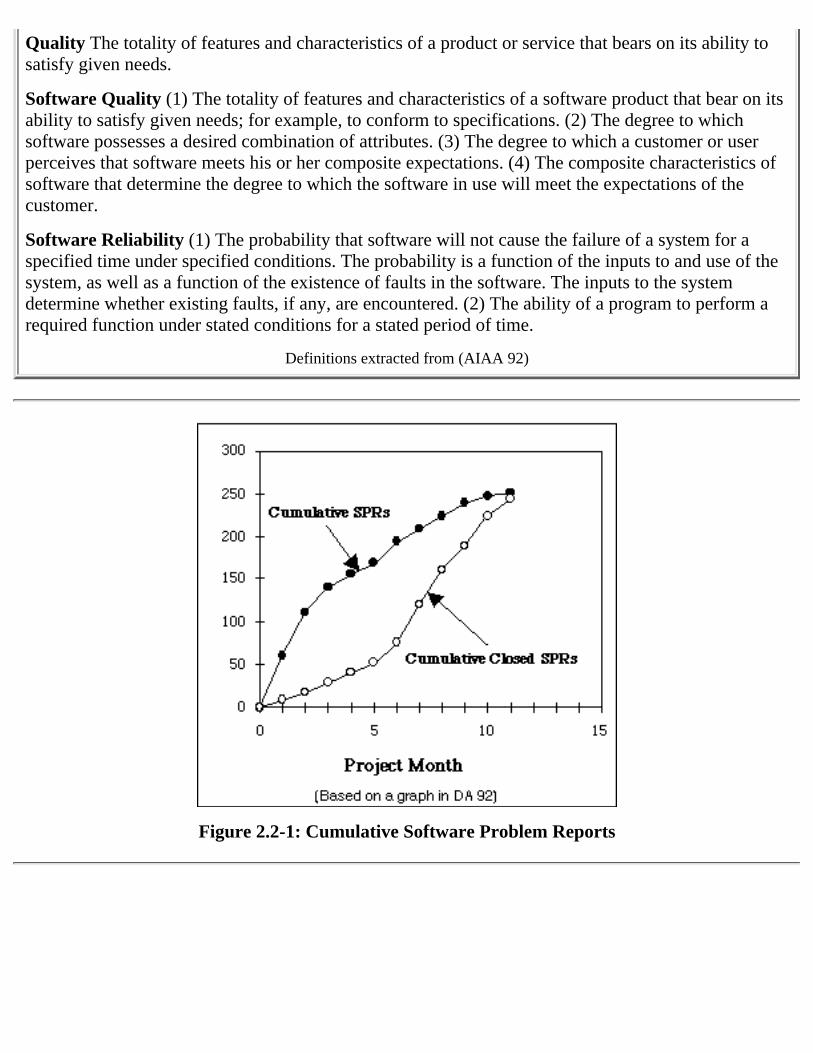
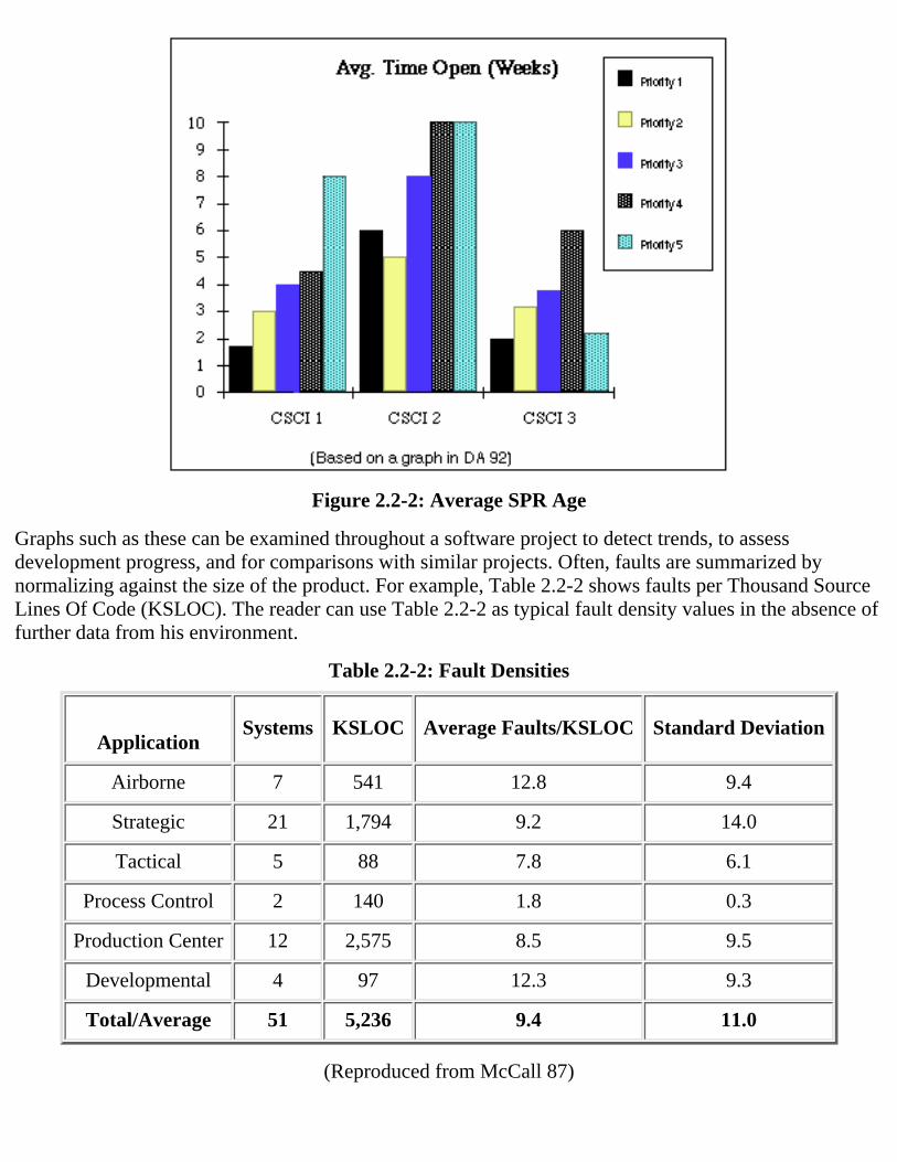
8 The graphs in Figures 2.2-1 and 2.2-2 are for illustration only, and do NOT show real data.
9 Many other models make this assumption. Others assume that faults that contribute more to the failurerate found earlier, or even more complicted relationships. These models do not exhibit a linearrelationship between the failure rate and the expected number of failures.
Use the "Back" button on your browser to return to the previous page.
Measures: The output produced for a unit input in a software organization.
Related Metrics: Size as measured by Function Points (FPs) or Source Lines of Code(SLOC), effort, schedule.
Applications: Assessing productivity of a project, new technologies, etc.; estimating size,effort, cost, and schedule in project planning.
Definition: FPs per person month or SLOC per person month. FPs are a weighted sum ofthe number of program inputs, outputs, user inquiries, files, and external interfaces.
Range:Productivity: From 2 to 23 FPs per Person Month with a median of 5.6 FPs perPerson Month, or from 80-400 SLOC per Person Month.
●
Size: From 100 to 2,300 FPs with a median of 993 FPs, or from 2 to 512 KSLOC.●
Function Point Conversion: From 6 to 320 SLOC per FP.●
Notes: FPs are most applicable to Management Information Systems (MIS) and otherbusiness applications.
For More Information:
International Function Points User Group (IFPUG)5009-28 Pine Creek Drive
Productivity, the output produced for a unit of input, is a crucial measure for software organizations.Management cannot assess the worth of process improvement efforts and the impact of new tools,techniques, and methodologies without some mechanism for measuring productivity, as well as quality.Software system size and productivity are often useful in project planning. Budgets and schedules can beestimated from size measures. Ideally, a size measure should be easily estimated in the requirements
Source Lines Of Code (SLOC) is an early measure of the software size, and a number of cost modelswere developed on this basis2. Although relating to a software engineering perspective, this measure hasa number of paradoxes. Functionally equivalent systems can vary in SLOC, depending on how tightlycode is developed. Hence, measuring productivity by SLOC per person month rewards inefficient andsloppy coding. The expressiveness of source code varies with language level. Software can usually becoded in a higher level language with less SLOC. If used incautiously, SLOC productivity measures canshow decreased productivity when, in fact, productivity has increased (Jones 86). Finally, estimates ofSLOC made early in the lifecycle can exhibit great variability and may be inappropriate as the principaldriver to a software cost model.
Allan Albrecht (79), collaborating with John Gaffney, Jr. (Albrecht 83), designed Function Points (FPs)to be a direct measure of functionality capable of measurement from data typically available during therequirements phase. Use of FPs is becoming more widespread, particularly among software costmodelers. FPs are most appropriate for information systems, but modifications have been proposed toadapt them for more general applications. For example, Capers Jones' Feature Points accounts for thealgorithmic complexity typical of embedded systems.
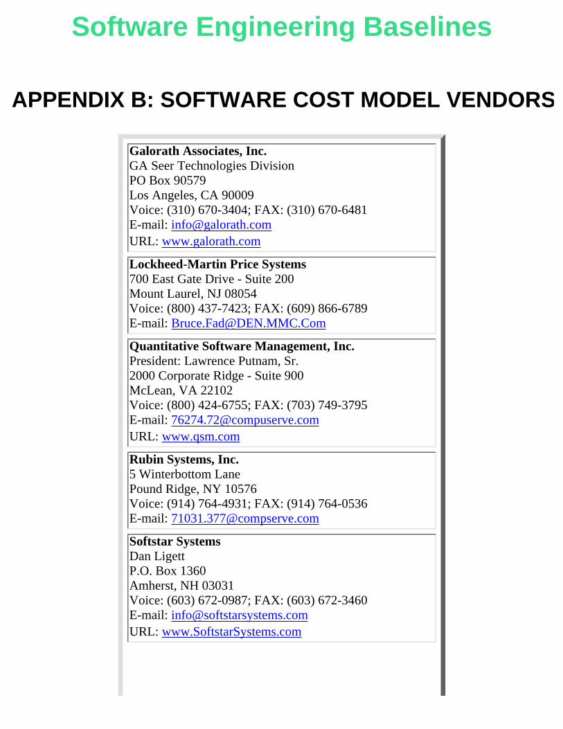
This report presents engineering norms for software productivity in two forms. Section 2.1.1 discussionsproductivity with FP measures. Section 2.1.2 uses the more traditional SLOC measures. A number ofsoftware cost model vendors and consultants on software productivity measurement maintain proprietarydatabases. Appendix B lists contact information for the most well-known vendors.
2.1.1 Functions Points
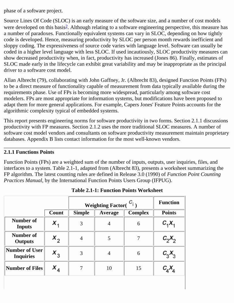
Function Points (FPs) are a weighted sum of the number of inputs, outputs, user inquiries, files, andinterfaces to a system. Table 2.1-1, adapted from (Albrecht 83), presents a worksheet summarizing theFP algorithm. The latest counting rules are defined in Release 3.0 (1990) of Function Point CountingPractices Manual, by the International Function Points Users Group (IFPUG).
Table 2.1-1: Function Points Worksheet
Weighting Factor( ) Function
Count Simple Average Complex Points
Number ofInputs 3 4 6
Number ofOutputs 4 5 7
Number of UserInquiries 3 4 6
Number of Files 7 10 15
Number ofExternal
Interfaces5 7 10
Total Function Points
What are typical system sizes for systems in terms of FPs? Two small datasets seem to be frequentlyreferenced by FP researchers - Allan Albrecht & John Gaffney's (Albrecht 83) and Chris Kemerer's(Kemerer 87). These datasets contain mostly business applications written in Cobol. Cost modelingvendors have developed their own databases, but these are proprietary and not generally available.
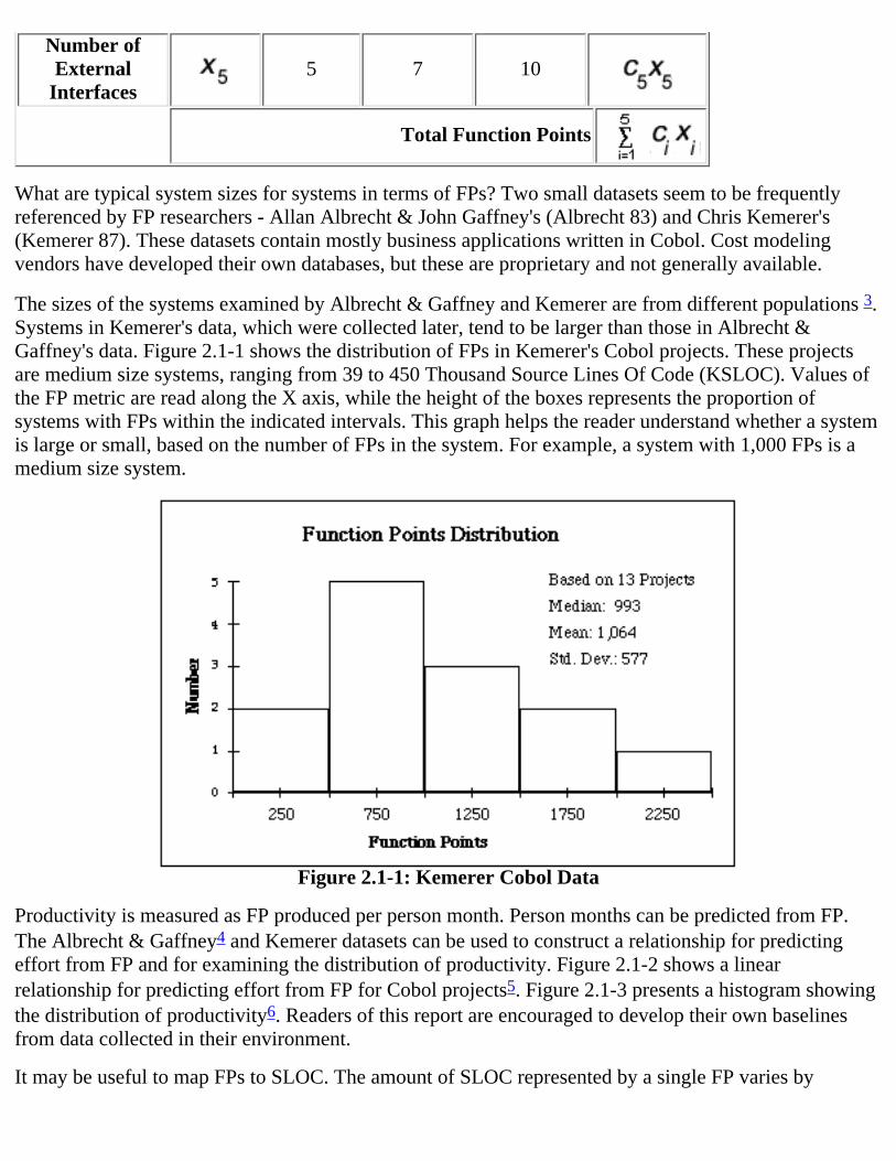
The sizes of the systems examined by Albrecht & Gaffney and Kemerer are from different populations 3.Systems in Kemerer's data, which were collected later, tend to be larger than those in Albrecht &Gaffney's data. Figure 2.1-1 shows the distribution of FPs in Kemerer's Cobol projects. These projectsare medium size systems, ranging from 39 to 450 Thousand Source Lines Of Code (KSLOC). Values ofthe FP metric are read along the X axis, while the height of the boxes represents the proportion ofsystems with FPs within the indicated intervals. This graph helps the reader understand whether a systemis large or small, based on the number of FPs in the system. For example, a system with 1,000 FPs is amedium size system.
Figure 2.1-1: Kemerer Cobol Data
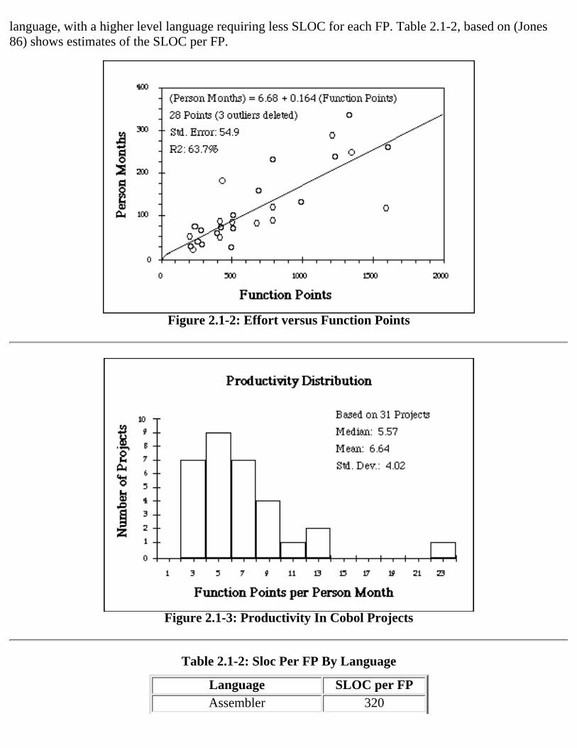
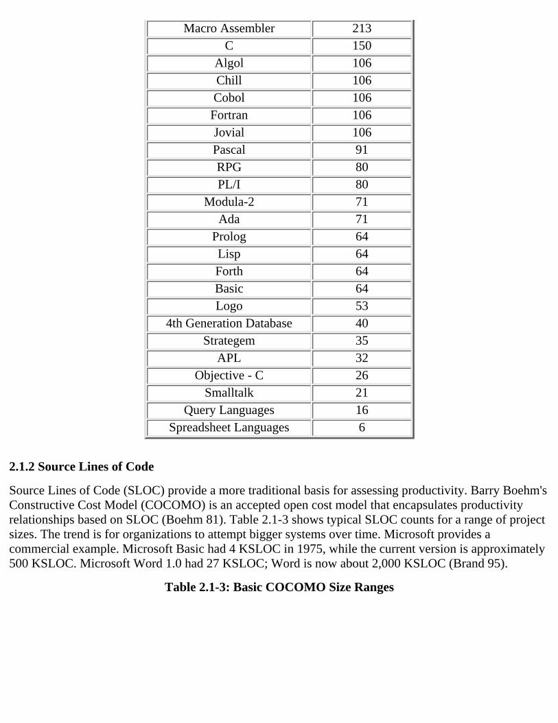
Productivity is measured as FP produced per person month. Person months can be predicted from FP.The Albrecht & Gaffney4 and Kemerer datasets can be used to construct a relationship for predictingeffort from FP and for examining the distribution of productivity. Figure 2.1-2 shows a linearrelationship for predicting effort from FP for Cobol projects5. Figure 2.1-3 presents a histogram showingthe distribution of productivity6. Readers of this report are encouraged to develop their own baselinesfrom data collected in their environment.
It may be useful to map FPs to SLOC. The amount of SLOC represented by a single FP varies by
language, with a higher level language requiring less SLOC for each FP. Table 2.1-2, based on (Jones86) shows estimates of the SLOC per FP.
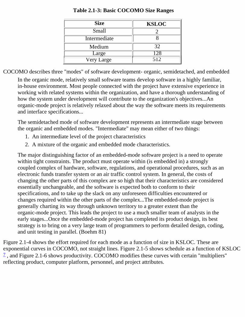
Source Lines of Code (SLOC) provide a more traditional basis for assessing productivity. Barry Boehm'sConstructive Cost Model (COCOMO) is an accepted open cost model that encapsulates productivityrelationships based on SLOC (Boehm 81). Table 2.1-3 shows typical SLOC counts for a range of projectsizes. The trend is for organizations to attempt bigger systems over time. Microsoft provides acommercial example. Microsoft Basic had 4 KSLOC in 1975, while the current version is approximately500 KSLOC. Microsoft Word 1.0 had 27 KSLOC; Word is now about 2,000 KSLOC (Brand 95).
Table 2.1-3: Basic COCOMO Size Ranges
Very Large 512
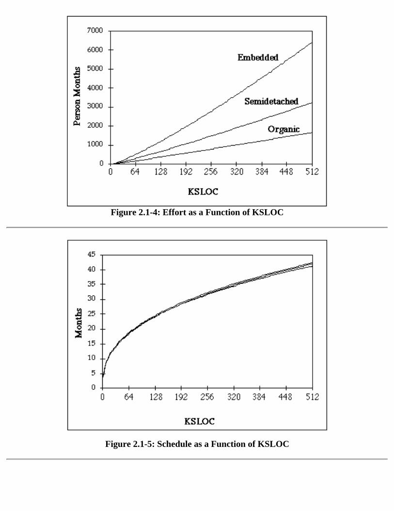
COCOMO describes three "modes" of software development- organic, semidetached, and embedded
In the organic mode, relatively small software teams develop software in a highly familiar,in-house environment. Most people connected with the project have extensive experience inworking with related systems within the organization, and have a thorough understanding ofhow the system under development will contribute to the organization's objectives...Anorganic-mode project is relatively relaxed about the way the software meets its requirementsand interface specifications...
The semidetached mode of software development represents an intermediate stage betweenthe organic and embedded modes. "Intermediate" may mean either of two things:
An intermediate level of the project characteristics1.
A mixture of the organic and embedded mode characteristics.2.
The major distinguishing factor of an embedded-mode software project is a need to operatewithin tight constraints. The product must operate within (is embedded in) a stronglycoupled complex of hardware, software, regulations, and operational procedures, such as anelectronic funds transfer system or an air traffic control system. In general, the costs ofchanging the other parts of this complex are so high that their characteristics are consideredessentially unchangeable, and the software is expected both to conform to theirspecifications, and to take up the slack on any unforeseen difficulties encountered orchanges required within the other parts of the complex...The embedded-mode project isgenerally charting its way through unknown territory to a greater extent than theorganic-mode project. This leads the project to use a much smaller team of analysts in theearly stages...Once the embedded-mode project has completed its product design, its beststrategy is to bring on a very large team of programmers to perform detailed design, coding,and unit testing in parallel. (Boehm 81)
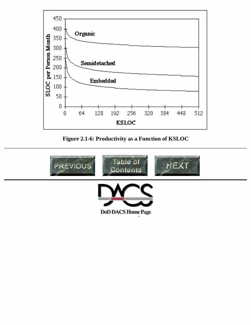
Figure 2.1-4 shows the effort required for each mode as a function of size in KSLOC. These areexponential curves in COCOMO, not straight lines. Figure 2.1-5 shows schedule as a function of KSLOC7 , and Figure 2.1-6 shows productivity. COCOMO modifies these curves with certain "multipliers"reflecting product, computer platform, personnel, and project attributes.
Source: Original sources are by Zygmund Jelinski and Paul Moranda (1972) and by Martin Shooman(1972).
Measures: User-oriented quality as shown by failure behavior of a system.
Related Metrics: Mean Time Between Failure (MTBF), Failure Intensity, Failure Rate, Fault Density
Applications: Quality assurance, planning and monitoring system testing, operations andmaintenance planning.
Definition: The probability that software will not cause the failure of a system for a specified timeunder specified conditions. The probability is a function of the inputs to and use of the system, as wellas a function of the existence of faults in the software. The inputs to the system determine whetherexisting faults, if any, are encountered.
Range:Operational failure rate ranges at least from 3x10⁻⁶ to 55x10-6 Failures per CPU Second.MTBF ranges at least from 5.1 to 92.6 CPU hours.
Fault density at the start of System Test ranges from 1 to 10 Faults per KSLOC, with anaverage of 6 Faults per KSLOC. KSLOC is counted here as delivered executable sourcelines, excluding reused code, data declarations, comments, etc.
Expected number of faults removed per failure: 0.955 Faults
For More Information:
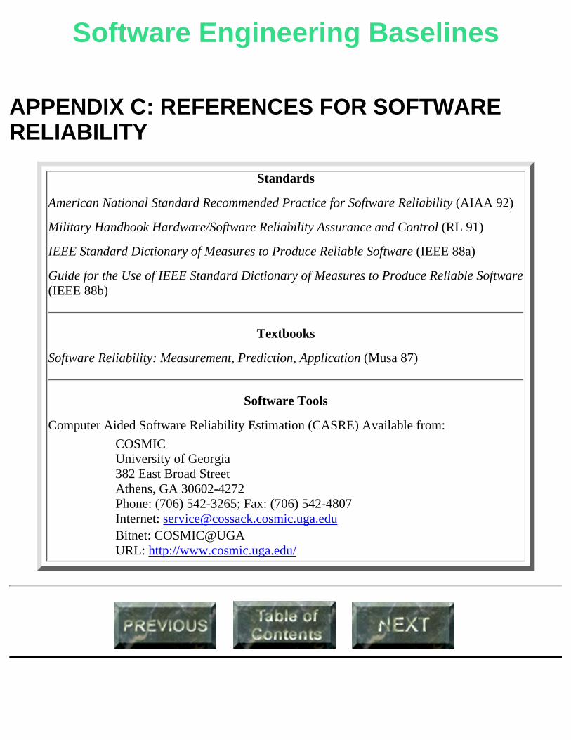
John D. Musa, Anthony Iannino, and Kazuhira Okumoto, Software Reliability: Measurement,Prediction, Application, McGraw-Hill, 1987.
American National Standard Recommended Practice for Software Reliability, American Institute ofAeronautics and Astronautics, ANSI/AIAA R-013-1992; February 23, 1993.
Although many factors are used to describe software quality - for example, portability, usability, andmaintainability - reliability is most commonly used. Because it is based on the occurrence of observableproblems or failures in the product, it is among the easiest of the quality factors to measure. It is also aneasy concept for a user to relate to - the user expects the product to be error free, thus, highly reliable.Maintainability and availability are two other quality factors closely related to reliability. Maintainabilityis often measured by Mean Time To Repair (MTTR) and availability by the ratio of the Mean Time
Between Failures (MTBF) to the sum of MTBF and MTTR. The calculation of each of these is again,based on tracking failures.
Reliability is one of the best known and oldest metrics. Software managers typically tracked softwarebugs even before software reliability concepts were explicitly formalized. Collecting and trackingso-called Software Problem Reports (SPRs) or Software Trouble Reports (STRs) is still a commonprocedure for monitoring the software development process to achieve reliability goals (Section 2.2.1).Additionally, much work since the seventies has been directed toward conceptual clarification andmodeling of software reliability. This has produced a consensus view of the software failure process,which is reflected in the definitions in Table 2.2-1. Basically, failures, observed while operatingsoftware, are caused when the software enters a state in which a fault or defect in the product changes theresulting output. Since inputs, which effect state changes, and the location of faults are not completelyknown a priori, software reliability is modeled as a stochastic process. This conceptual understandingprovides the foundation for an engineering technology for modeling and controlling software reliability(Section 2.2.2), as well as procedures for predicting reliability (Section 2.2.3). This technology can onlybe presented very briefly here. Appendix C provides additional resources for Software ReliabilityEngineering.
2.2.1 Fault Profiles
Reliability was originally monitored by tracking faults found throughout the lifecycle. Faults arecollected and cataloged in forms known by various names, such as Software Trouble Reports (STRs) orSoftware Problem Reports (SPRs). Various graphical displays of SPR data can provide managementinsight into the software development process. For example, Figures 2.2-1 and 2.2-2 show two of fivegraphs defined by the United States Army's Software Test and Evaluation Panel (STEP) "Fault Profiles"metric8.
Table 2.2-1: Definitions for Software Reliability
Error (1) A discrepancy between a computed, observed or measured value or condition and the true,specified or theoretically correct value or condition. (2) Human action that results in softwarecontaining a fault. Examples include omission or misinterpretation of user requirements in a softwarespecification, and incorrect translation or omission of a requirement in the design specification. Thisis not a preferred usage.
Failure (1) The inability of a system or system component to perform a required function withspecified limits. A failure may be produced when a fault is encountered and a loss of the expectedservice to the user results. (2) The termination of the ability of a functional unit to perform its requiredfunction. (3) A departure of program operation from program requirements.
Failure Rate (1) The ratio of the number of failures of a given category or severity to a given periodof time; for example, failures per month. Synonymous with failure intensity. (2) The ratio of thenumber of failures to a given unit of measure; for example, failures per unit of time, failures pernumber of transactions, failures per number of computer runs.
Fault (1) A defect in the code that can be the cause of one or more failures. (2) An accidentalcondition that causes a functional unit to fail to perform its required function. Synonymous with bug.
Quality The totality of features and characteristics of a product or service that bears on its ability tosatisfy given needs.
Software Quality (1) The totality of features and characteristics of a software product that bear on itsability to satisfy given needs; for example, to conform to specifications. (2) The degree to whichsoftware possesses a desired combination of attributes. (3) The degree to which a customer or userperceives that software meets his or her composite expectations. (4) The composite characteristics ofsoftware that determine the degree to which the software in use will meet the expectations of thecustomer.
Software Reliability (1) The probability that software will not cause the failure of a system for aspecified time under specified conditions. The probability is a function of the inputs to and use of thesystem, as well as a function of the existence of faults in the software. The inputs to the systemdetermine whether existing faults, if any, are encountered. (2) The ability of a program to perform arequired function under stated conditions for a stated period of time.
Definitions extracted from (AIAA 92)
Figure 2.2-1: Cumulative Software Problem Reports
Figure 2.2-2: Average SPR Age
Graphs such as these can be examined throughout a software project to detect trends, to assessdevelopment progress, and for comparisons with similar projects. Often, faults are summarized bynormalizing against the size of the product. For example, Table 2.2-2 shows faults per Thousand SourceLines Of Code (KSLOC). The reader can use Table 2.2-2 as typical fault density values in the absence offurther data from his environment.
Table 2.2-2: Fault Densities
ApplicationSystems KSLOC Average Faults/KSLOC Standard Deviation
Airborne 7 541 12.8 9.4
Strategic 21 1,794 9.2 14.0
Tactical 5 88 7.8 6.1
Process Control 2 140 1.8 0.3
Production Center 12 2,575 8.5 9.5
Developmental 4 97 12.3 9.3
Total/Average 51 5,236 9.4 11.0
(Reproduced from McCall 87)
2.2.2 Software Reliability Engineering
While tracking Software Problem Reports is a useful methodology for monitoring the softwaredevelopment process, it does not result in a predictive user-oriented reliability metric. Software reliabilitymodels, which relate failure data to a statistical model of the software failure process, are used to specify,predict, estimate, and assess the reliability of software systems.
The discipline of Software Reliability Engineering evolved from the development and application ofthese probabilistic models of the software failure process.
Many models are in use with good results. Customarily, these models are applied during system test ormaintenance by collecting failure data, fitting the model, and updating results based on additional data. Ifthe fit is good, the model can be used with relative confidence to provide an assessment of currentreliability or to predict future failure behavior. For example, if a model has been proven accurate timeand again for previous increments of a software product, then its use results in trust in new results. Forexplicitness, this report describes Musa's Basic Execution Time Model, one of the most well-acceptedsoftware reliability models.
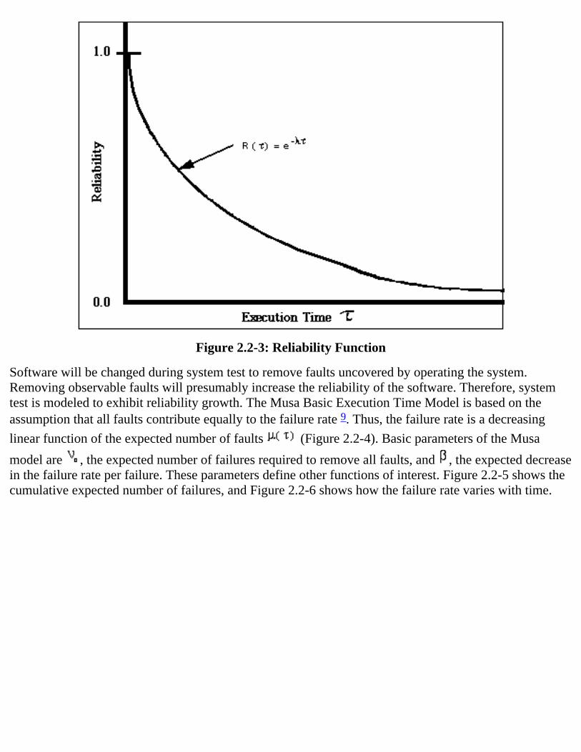
Suppose a software system is operating in an environment with an unchanging operational profile. Inother words, the distribution of the types of user demands or requests for system capabilities do not varywith time (Musa 93). Furthermore, suppose no changes are made to the software during operations. Thenthe software might be modeled with a constant failure rate . Then the expected number of failures in atime interval is proportional to the length of that time interval. The probability that the software willoperate without failure, the reliability R( ), becomes smaller the longer the time period underconsideration. Figure 2.2-3 shows this relationship in which reliability decreases exponentially withexecution time . For systems with a constant failure rate, the Mean Time Between Failure, calculated asthe reciprocal of the failure rate, is often used to summarize reliability.
Figure 2.2-3: Reliability Function
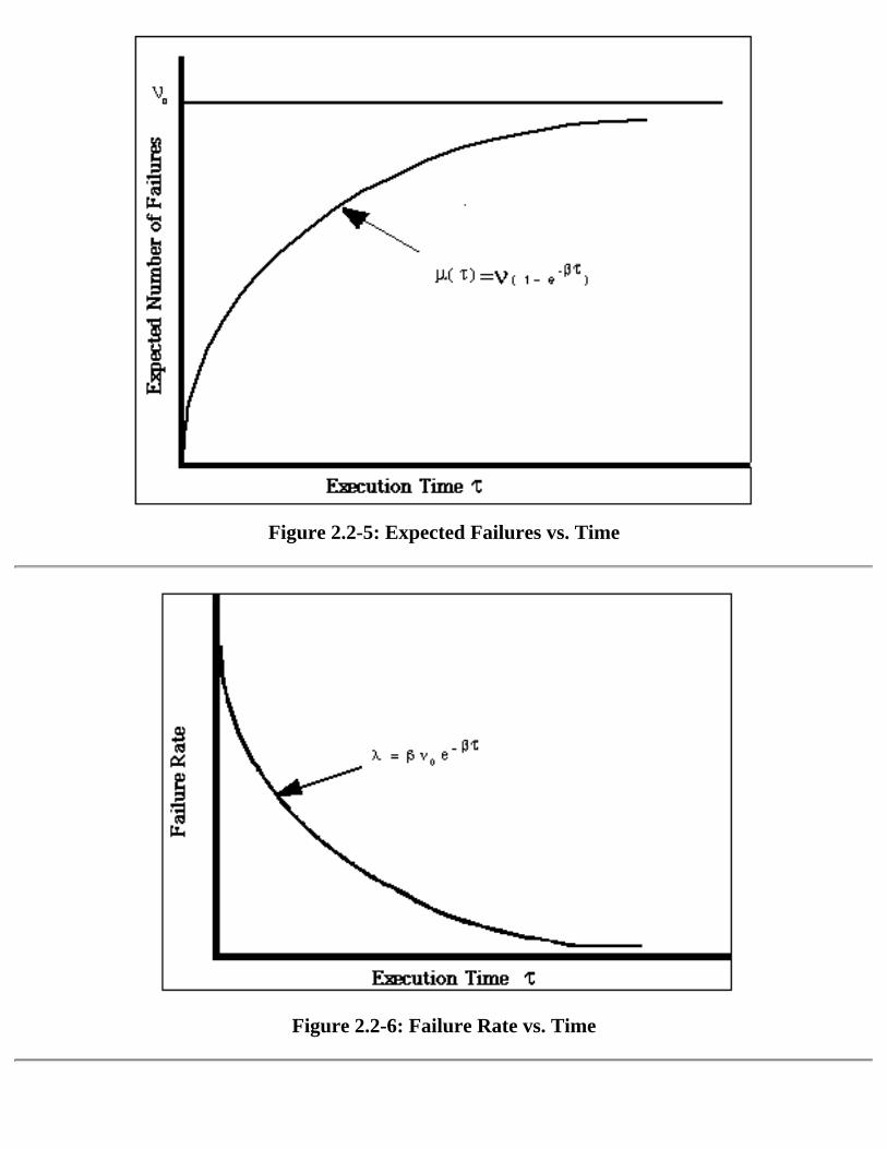
Software will be changed during system test to remove faults uncovered by operating the system.Removing observable faults will presumably increase the reliability of the software. Therefore, systemtest is modeled to exhibit reliability growth. The Musa Basic Execution Time Model is based on theassumption that all faults contribute equally to the failure rate 9. Thus, the failure rate is a decreasing
linear function of the expected number of faults (Figure 2.2-4). Basic parameters of the Musa
model are , the expected number of failures required to remove all faults, and , the expected decreasein the failure rate per failure. These parameters define other functions of interest. Figure 2.2-5 shows thecumulative expected number of failures, and Figure 2.2-6 shows how the failure rate varies with time.
Figure 2.2-4: Failure Rate vs. Expected Failures
Given the parameters of the model, and , one can determine how long system test must proceeduntil any reliability goal is met. Confidence bounds should be used for a reliability stopping rule insteadof point estimates. For example, testing might stop when a 90% upper confidence bound on the numberof remaining failures is below a required target bound. Alternatively, testing could stop when totallifecycle cost is minimized. The cost of a failure is greater in the field than in system test. The marginalbenefit of testing for an increment of execution time is the expected decrease in the cost of failure,accounting for the expected number of failures in that increment. The marginal cost of testing is theresources needed to test for an increment of execution time. To minimize total cost, testing shouldproceed until the marginal benefit falls below the marginal cost (Vienneau 91).
Figure 2.2-5: Expected Failures vs. Time
Figure 2.2-6: Failure Rate vs. Time
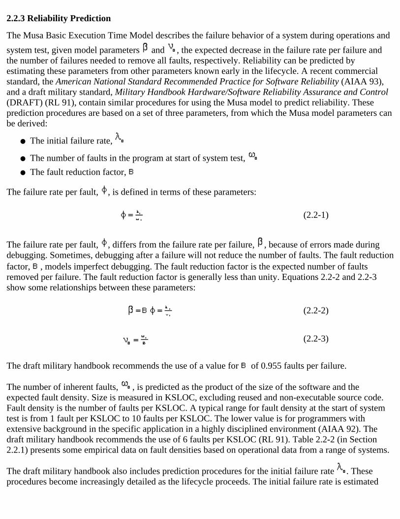
2.2.3 Reliability Prediction
The Musa Basic Execution Time Model describes the failure behavior of a system during operations and
system test, given model parameters and , the expected decrease in the failure rate per failure andthe number of failures needed to remove all faults, respectively. Reliability can be predicted byestimating these parameters from other parameters known early in the lifecycle. A recent commercialstandard, the American National Standard Recommended Practice for Software Reliability (AIAA 93),and a draft military standard, Military Handbook Hardware/Software Reliability Assurance and Control(DRAFT) (RL 91), contain similar procedures for using the Musa model to predict reliability. Theseprediction procedures are based on a set of three parameters, from which the Musa model parameters canbe derived:
The initial failure rate, ●
The number of faults in the program at start of system test, ●
The fault reduction factor, ●
The failure rate per fault, , is defined in terms of these parameters:
(2.2-1)
The failure rate per fault, , differs from the failure rate per failure, , because of errors made duringdebugging. Sometimes, debugging after a failure will not reduce the number of faults. The fault reductionfactor, , models imperfect debugging. The fault reduction factor is the expected number of faultsremoved per failure. The fault reduction factor is generally less than unity. Equations 2.2-2 and 2.2-3show some relationships between these parameters:
(2.2-2)
(2.2-3)
The draft military handbook recommends the use of a value for of 0.955 faults per failure.
The number of inherent faults, , is predicted as the product of the size of the software and theexpected fault density. Size is measured in KSLOC, excluding reused and non-executable source code.Fault density is the number of faults per KSLOC. A typical range for fault density at the start of systemtest is from 1 fault per KSLOC to 10 faults per KSLOC. The lower value is for programmers withextensive background in the specific application in a highly disciplined environment (AIAA 92). Thedraft military handbook recommends the use of 6 faults per KSLOC (RL 91). Table 2.2-2 (in Section2.2.1) presents some empirical data on fault densities based on operational data from a range of systems.
The draft military handbook also includes prediction procedures for the initial failure rate . Theseprocedures become increasingly detailed as the lifecycle proceeds. The initial failure rate is estimated
during the requirements phase:
(2.2-4)
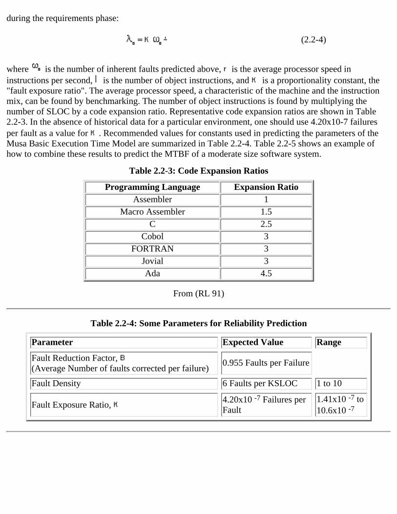
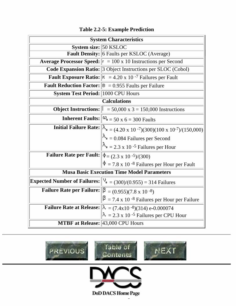
where is the number of inherent faults predicted above, is the average processor speed ininstructions per second, is the number of object instructions, and is a proportionality constant, the"fault exposure ratio". The average processor speed, a characteristic of the machine and the instructionmix, can be found by benchmarking. The number of object instructions is found by multiplying thenumber of SLOC by a code expansion ratio. Representative code expansion ratios are shown in Table2.2-3. In the absence of historical data for a particular environment, one should use 4.20x10⁻⁷ failuresper fault as a value for . Recommended values for constants used in predicting the parameters of theMusa Basic Execution Time Model are summarized in Table 2.2-4. Table 2.2-5 shows an example ofhow to combine these results to predict the MTBF of a moderate size software system.
Table 2.2-3: Code Expansion Ratios
Programming Language Expansion RatioAssembler 1
Macro Assembler 1.5C 2.5
Cobol 3FORTRAN 3
Jovial 3Ada 4.5
From (RL 91)
Table 2.2-4: Some Parameters for Reliability Prediction
Parameter Expected Value Range
Fault Reduction Factor, (Average Number of faults corrected per failure)
Measures: Size, control flow, data structures, intermodule structure, etc.
Related Metrics: Source Lines of Code (SLOC), McCabe's Cyclomatic Complexity metric,Halstead's Software Science metrics, Henry and Kafura's Information Flow metric, test coveragemetrics.
Applications: Quality assurance during development, prediction of operational characteristics, testplanning.
Definition: Cyclomatic complexity is the graph theoretical complexity of a computer program'sflowchart. In other words, the number of areas enclosed by a flowchart.
Range: Usually consciously determined by management decision. Cyclomatic complexity must bepositive with an upper bound of 10 being recommended.
Notes: Most well-developed for application to individual subroutines.
Productivity is chiefly a management concern, while reliability is a quality factor directly visible to usersof software systems. These externally visible attributes of software processes and products are stronglyinfluenced by engineering attributes of software such as complexity. Well-designed software exhibits aminimum of unnecessary complexity. Unmanaged complexity leads to software difficult to use,maintain, and modify. It causes increased development costs and overrun schedules. But certain elementsof software are inherently complex - conformance to arbitrary external interfaces, pressure to adapt tochanging user requirements, lack of obvious representations for visualizing software (Brooks 87).
Controlling and measuring complexity is a challenging engineering, management, and research problem.Metrics have been created for measuring various aspects of complexity such as sheer size, control flow,data structures, and intermodule structure. The most well-accepted are probably Source Lines of Code(Section 2.1.2) and Cyclomatic complexity (McCabe 76). Complexity metrics not otherwise discussedhere include Halstead's Software Science metrics and Henry and Kafura's Information Flow metric.Halstead's metrics are controversial. Henry and Kafura's metric is one of the first of a family addressingdesign complexity, the complexity embedded in connections among modules. Although important,measurement of this aspect of complexity, unlike the measurement of complexity within a single module,is still a research issue.
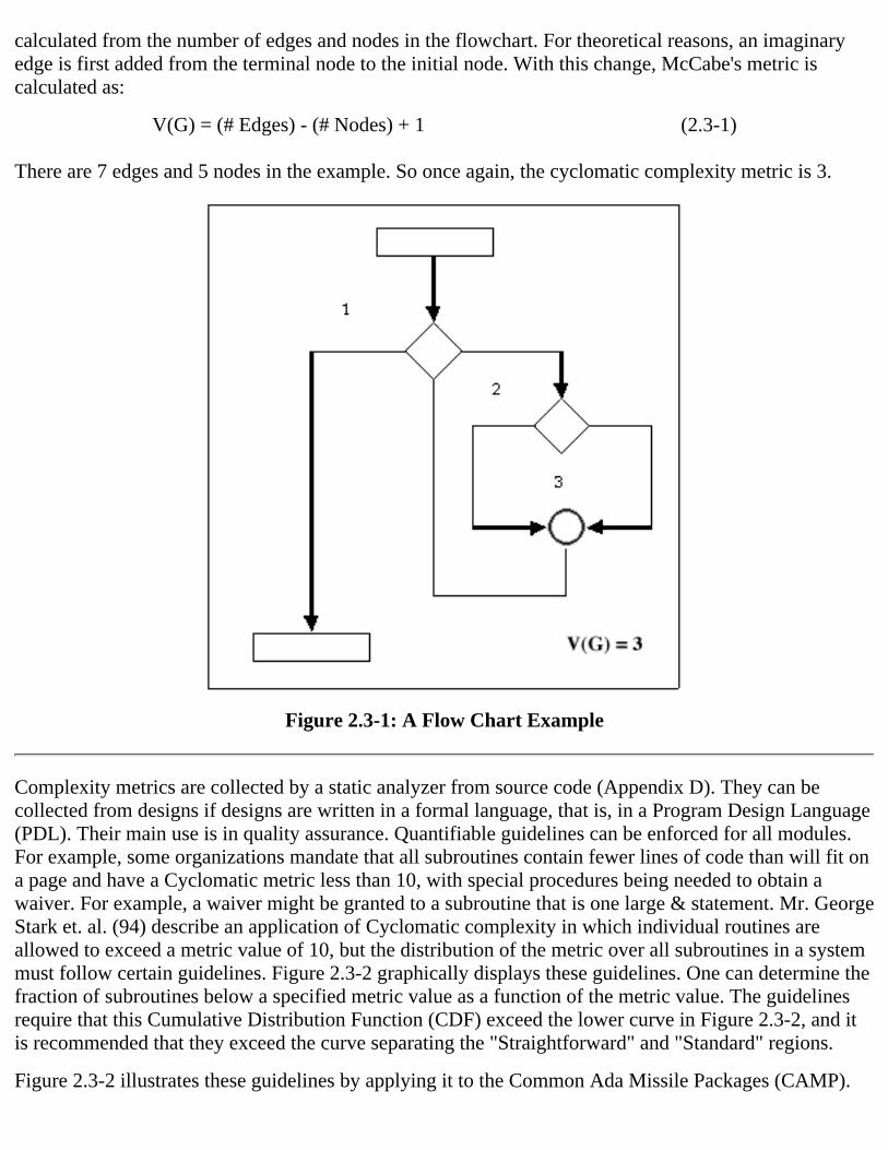
Cyclomatic complexity, V(G), applies graph theory to measure control flow complexity. Intuitively, themetric is the number of connected regions in a flowchart, for a subroutine with one entrance and one exit.Figure 2.3-1 shows a sample flowchart for which McCabe's metric is 3. McCabe's metric can also be
calculated from the number of edges and nodes in the flowchart. For theoretical reasons, an imaginaryedge is first added from the terminal node to the initial node. With this change, McCabe's metric iscalculated as:
V(G) = (# Edges) - (# Nodes) + 1 (2.3-1)
There are 7 edges and 5 nodes in the example. So once again, the cyclomatic complexity metric is 3.
Figure 2.3-1: A Flow Chart Example
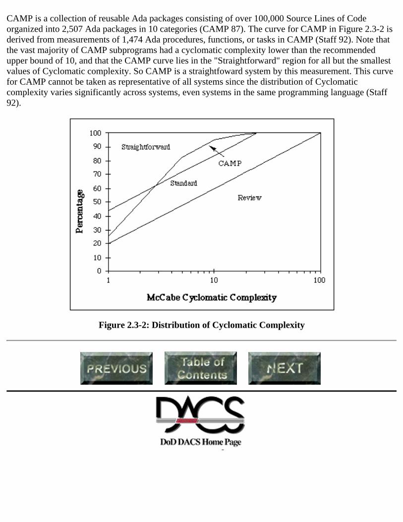
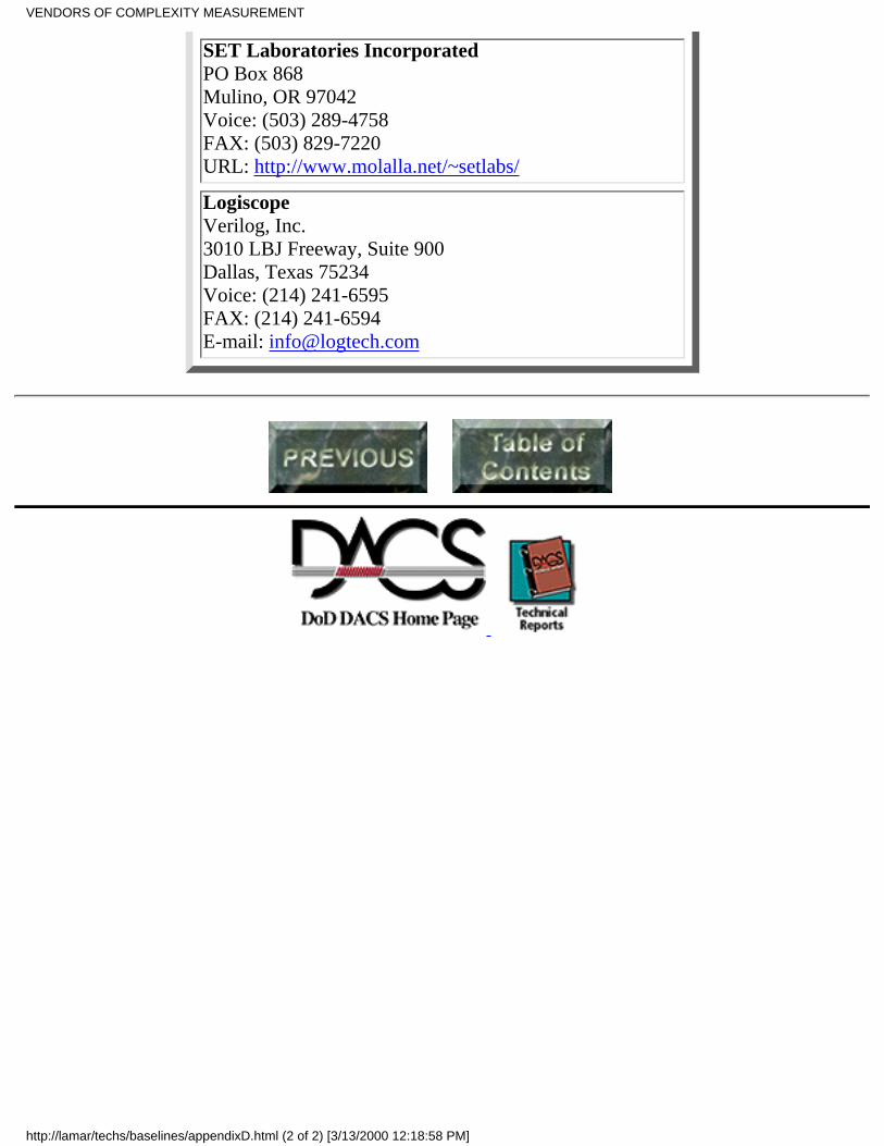
Complexity metrics are collected by a static analyzer from source code (Appendix D). They can becollected from designs if designs are written in a formal language, that is, in a Program Design Language(PDL). Their main use is in quality assurance. Quantifiable guidelines can be enforced for all modules.For example, some organizations mandate that all subroutines contain fewer lines of code than will fit ona page and have a Cyclomatic metric less than 10, with special procedures being needed to obtain awaiver. For example, a waiver might be granted to a subroutine that is one large & statement. Mr. GeorgeStark et. al. (94) describe an application of Cyclomatic complexity in which individual routines areallowed to exceed a metric value of 10, but the distribution of the metric over all subroutines in a systemmust follow certain guidelines. Figure 2.3-2 graphically displays these guidelines. One can determine thefraction of subroutines below a specified metric value as a function of the metric value. The guidelinesrequire that this Cumulative Distribution Function (CDF) exceed the lower curve in Figure 2.3-2, and itis recommended that they exceed the curve separating the "Straightforward" and "Standard" regions.
Figure 2.3-2 illustrates these guidelines by applying it to the Common Ada Missile Packages (CAMP).
CAMP is a collection of reusable Ada packages consisting of over 100,000 Source Lines of Codeorganized into 2,507 Ada packages in 10 categories (CAMP 87). The curve for CAMP in Figure 2.3-2 isderived from measurements of 1,474 Ada procedures, functions, or tasks in CAMP (Staff 92). Note thatthe vast majority of CAMP subprograms had a cyclomatic complexity lower than the recommendedupper bound of 10, and that the CAMP curve lies in the "Straightforward" region for all but the smallestvalues of Cyclomatic complexity. So CAMP is a straightfoward system by this measurement. This curvefor CAMP cannot be taken as representative of all systems since the distribution of Cyclomaticcomplexity varies significantly across systems, even systems in the same programming language (Staff92).
Figure 2.3-2: Distribution of Cyclomatic Complexity
3.0 REFERENCES(AFSC 87) Software Quality Indicators, AFSC Pamphlet 800-14, Air Force Systems Command, January1987.
(AFSC 88) Software Management Indicators, AFSC Pamphlet 800-43, Air Force Systems Command,June 1988.
(AIAA 93) American National Standard Recommended Practice for Software Reliability, AmericanInstitute of Aeronautics and Astronautics, ANSI/AIAA R-013-1992; February 23, 1993.
(Albrecht 79) Allan J. Albrecht, "Measuring Application Development Productivity," Proceedings of theIBM Application Development Symposium, Monterey, California, October 1979, pp. 83-92.
(Albrecht 83) Allan J. Albrecht and John E. Gaffney, Jr., "Software Function, Source Lines of Code, andDevelopment Effort Prediction: A Software Science Validation," IEEE Transactions on SoftwareEngineering, Volume SE-9, Number 6, November 1993, pp. 639-648.
(Brand 95) Stewart Brand, "The Physicist," Wired 3.09, September 1995.
(Boehm 81) Barry W. Boehm, Software Engineering Economics, Prentice-Hall, 1981.
(Brooks 87) Frederick P. Brooks, Jr., "No Silver Bullet," Computer, April 1987, pp. 10-19.
(Carleton 92) A. Carleton et al., Software Measurement for DOD Systems: Recommendations for InitialCore Measures, Software Engineering Institute, CMU/SEI-92-TR-19, 1992.
(CAMP 87) User's Guide for the Missile Software Parts of the Common Ada Missile Packages (CAMP)Project, McDonnell Douglas Astronautics Company, 30 October 1987.
(Chruscicki 95) Andrew J. Chruscicki and John J. Marciniak, National Software Initiative: Report of theCooperstown Workshops, Data & Analysis Center for Software, 7 June 1995.
(DA 92) "Software Test and Evaluation Guidelines," Test and Evaluation Procedures and Guidelines,Part Seven, (Draft), DA Pamphlet 73-1, Headquarters, Department of the Army, 30 September 1992.
(Grady 87) Robert B. Grady and Deborah L. Caswell, Software Metrics: Establishing a Company-WideProgram, Prentice-Hall, 1987.
(Grady 92) Robert B. Grady, Practical Software Metrics for Project Management and ProcessImprovement, Prentice-Hall, 1992.
(IEEE 88a) IEEE Standard Dictionary of Measures to Produce Reliable Software, Institute of Electricaland Electronics Engineers, IEEE Standard 981.1-1988.
(IEEE 88b) Guide for the Use of IEEE Standard Dictionary of Measures to Produce Reliable Software,Institute of Electrical and Electronics Engineers, IEEE 981.2-1988.
(Jelinski 72) Z. Jelinski and P. B. Moranda, "Software Reliability Research," Statistical ComputerPerformance Evaluation, Editor: W. Freidberger, Academic Press, 1972.
(Kemerer 87) Chris F. Kemerer, "An Empirical Validation of Software Cost Estimation Models,"Communications of the ACM, Volume 30, Number 5, May 1987, pp. 416-429.
(McCabe 76) Thomas McCabe, "A Software Complexity Measure," IEEE Transactions on SoftwareEngineering, Volume SE-2, December 1976, pp. 308-320.
(McCall 87) J. McCall et. al., Methodology for Software Reliability Prediction, (2 volumes), Rome AirDevelopment Center, RADC-TR-87-171, November 1987.
(Musa 87) John D. Musa, Anthony Iannino, and Kazuhira Okumoto, Software Reliability: Measurement,Prediction, Application, McGraw-Hill, 1987.
(Musa 93) John D. Musa, "Operational Profiles in Software-Reliability Engineering," IEEE Software,March 1993, pp. 14-32.
(Paulk 95) Mark C. Paulk et. al., The Capability Maturity Model: Guidelines for Improving the SoftwareProcess, Addison-Wesley, 1995.
(RL 91) Military Handbook Hardware/Software Reliability Assurance and Control, (DRAFT), RomeLaboratory, MIL-HDBK-XXX, 6 December 1991.
(Shooman 72) Martin L. Shooman, "Probabilistic Models for Software Reliability Prediction", StatisticalComputer Performance Evaluation, Editor: W. Freidberger, Academic Press, 1972.
(Springsteen 94) Beth Springsteen et al., Survey of Software Metrics in the Department of Defense andIndustry, IDA Paper P-2996, Institute for Defense Analysis, April 1994.
(Staff 92) Staff, Ada Usage Profiles, Kaman Sciences Corporation, October 30, 1992.
(Stark 94) George Stark, Robert C. Durst, and C. W. Vowell, "Using Metrics in Management DecisionMaking," Computer, September 1994, pp. 42-48.
(Vienneau 91) Robert L. Vienneau, "The Cost of Testing Software," Annual Reliability andMaintainability Symposium; Orlando, FL; January 29-31, 1991.
(Vienneau 95) Robert L. Vienneau, "The Present Value of Software Maintenance," Journal ofParametrics, Volume XV, Number 1, April 1995, pp. 18-36.
Software Engineering Baselines
APPENDIX A: ACRONYMSANOVA - Analysis Of Variance
CAMP - Common Ada Missile Packages
CDF - Cumulative Distribution Function
CMM - Capability Maturity Model
COCOMO - Constructive Cost Model
CPU - Central Processing Unit
CSC - Computer Sciences Corporation
CSCI - Computer Software Configuration Item
CSU - Computer Software Unit
DoD - Department of Defense
FP - Function Point
GSFC - Goddard Space Flight Center
IFPUG - International Function Points User's Group
KSLOC - Thousands of Source Lines of Code
MIS - Management Information System
MTBF - Mean Time Between Failures
MTTR - Mean Time To Repair
NASA/SEL - National Aeronautics and Space Administration Software Engineering Laboratory
NSDIR - National Software Data and Information Repository
PDL - Program Design Language
PIP - Process Improvement Paradigm
PSM - Practical Software Measurement
SEI - Software Engineering Institute
SEMA - Software Engineering Measurement and Analysis
2.2-4. Some Parameters for Reliability Prediction●
2.2-5. Example Prediction●
LIST OF FIGURES
2.1-1. Kemerer Cobol Data●
2.1-2. Effort versus Function Points●
2.1-3. Productivity In Cobol Projects●
2.1-4. Effort as a Function of KSLOC●
2.1-5. Schedule as a Function of KSLOC●
2.1-6. Productivity as a Function of KSLOC●
2.2-1. Cumulative Software Problem Reports●
2.2-2. Average SPR Age 20.●
2.2-3. Reliability Function●
2.2-4. Failure Rate vs. Expected Failures●
2.2-5. Expected Failures vs. Time●
2.2-6. Failure Rate vs. Time●
2.3-1. A Flow Chart Example●
2.3-2. Distribution of Cyclomatic Complexity●
Software Engineering Baselines
APPENDIX D: SOME VENDORS OF COMPLEXITYMEASUREMENT TOOLS
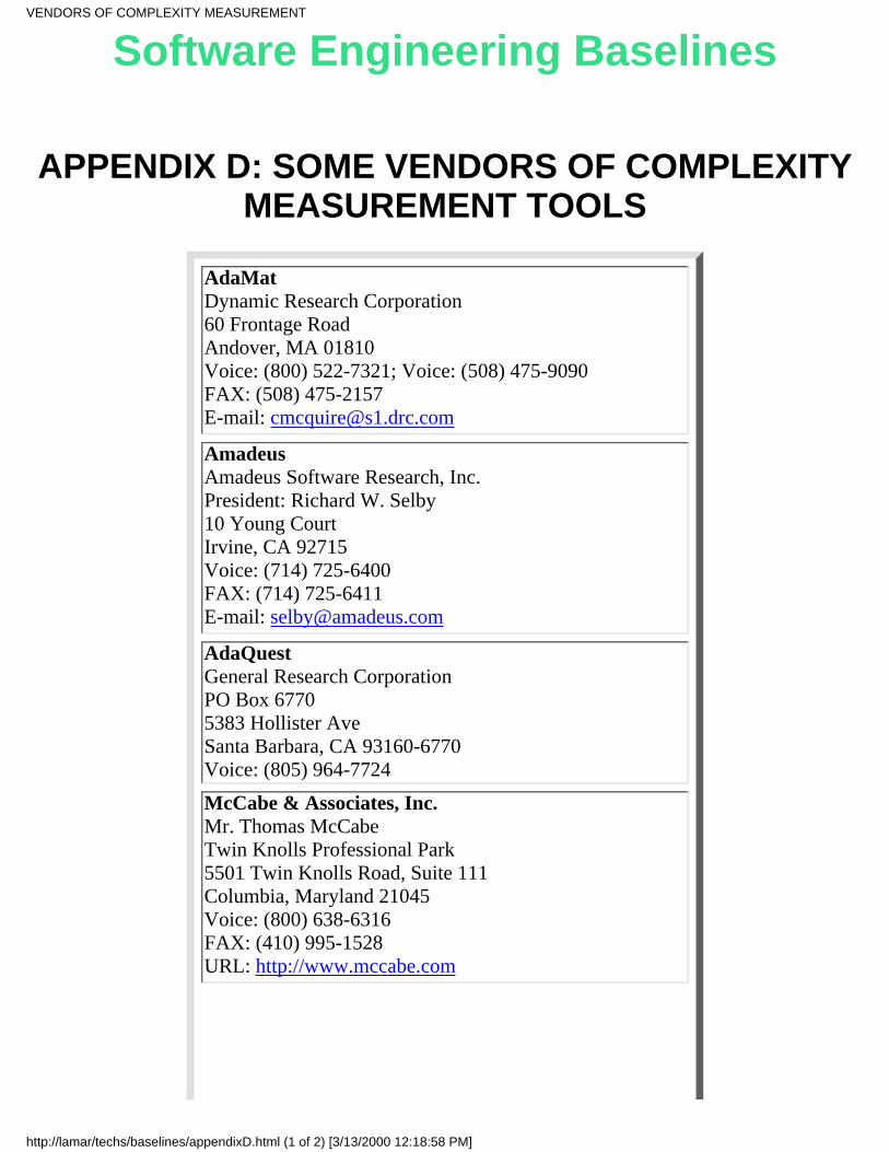
AdaMatDynamic Research Corporation60 Frontage RoadAndover, MA 01810Voice: (800) 522-7321; Voice: (508) 475-9090FAX: (508) 475-2157E-mail: [email protected]
AmadeusAmadeus Software Research, Inc.President: Richard W. Selby10 Young CourtIrvine, CA 92715Voice: (714) 725-6400FAX: (714) 725-6411E-mail: [email protected]
AdaQuestGeneral Research CorporationPO Box 67705383 Hollister AveSanta Barbara, CA 93160-6770Voice: (805) 964-7724
McCabe & Associates, Inc.Mr. Thomas McCabeTwin Knolls Professional Park5501 Twin Knolls Road, Suite 111Columbia, Maryland 21045Voice: (800) 638-6316FAX: (410) 995-1528URL: http://www.mccabe.com
VENDORS OF COMPLEXITY MEASUREMENT
http://lamar/techs/baselines/appendixD.html (1 of 2) [3/13/2000 12:18:58 PM]
Abstract:Software measurement programs are of increasing interest in the DoD and industrial practice. Theseprograms run the gamut of scope and purpose. The programs support the implementation andmanagement of process improvement programs.
The purpose of this report is to provide baseline information about a selected set of metrics, specificallyproductivity, complexity, and reliability. The question of what is an accepted value for a metric oftenarises when planning or implementing a project. A planner or manager may want to know what theexpected value should be for the complexity of the design or implemented code, or the expectedproductivity of the development life cycle.
Productivity, reliability, and complexity metrics are presented in the report. Definitions and the range ofvalues that may be expected based on current practice are provided for each metric. The examples areillustrative of commonly accepted or popular metrics for each area, but not the only metrics for eacharea. As additional data is collected and made available we hope to enhance this report to form a growingbase of norms for measurement practice.
Ordering Information:A bound version of this report, (see full table of contents) is avaliable for $30 and may be ordered fromthe DACS Product Orderform.