92
Software Estimation Software Estimation Thanks to Prof. Sharad Malik at Princeton University and Prof. Reinhard Wilhelm at Universitat des Saarlandes for some of the slides
| Date post: | 20-Dec-2015 |
| Category: |
Documents |
| View: | 214 times |
| Download: | 0 times |
Software EstimationSoftware Estimation
Thanks to Prof. Sharad Malik at Princeton Universityand Prof. Reinhard Wilhelm at Universitat des Saarlandes
for some of the slides
2
OutlineOutline
SW estimation overviewSW estimation overview
Program path analysisProgram path analysis
Micro-architecture modelingMicro-architecture modeling
Implementation examples: CinderellaImplementation examples: Cinderella
SW estimation in VCCSW estimation in VCC
SW estimation in AISW estimation in AI
SW estimation in POLISSW estimation in POLIS
3
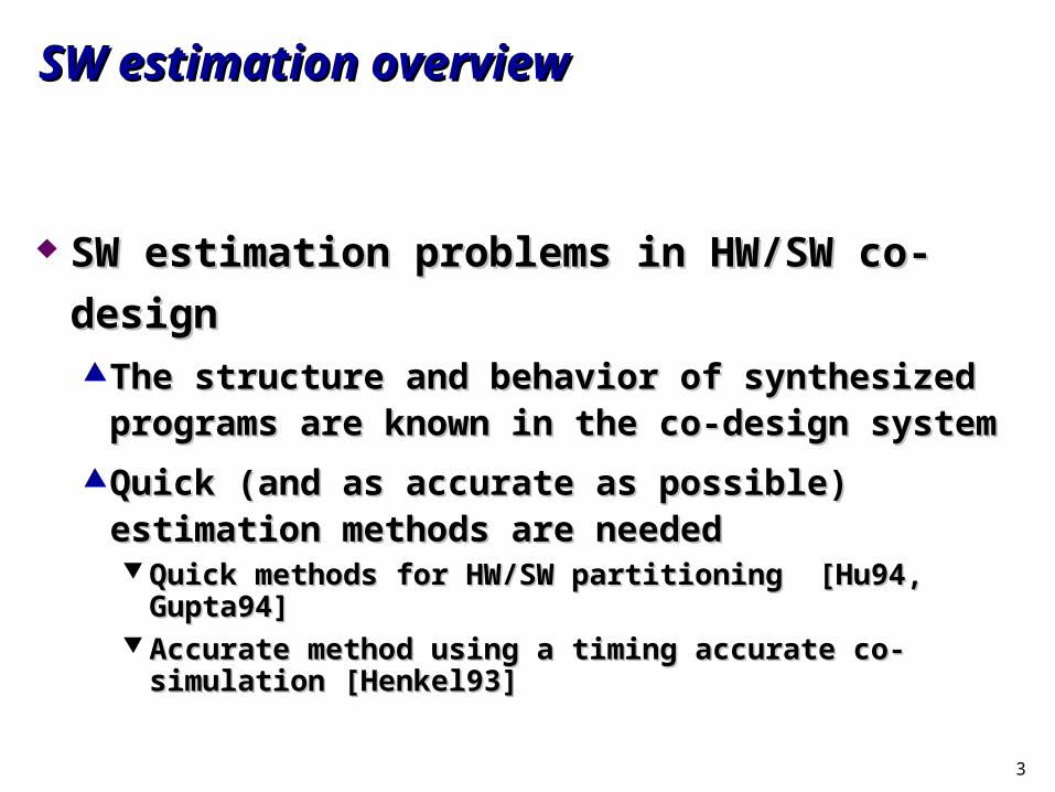
SW estimation overviewSW estimation overview
SW estimation problems in HW/SW co-designSW estimation problems in HW/SW co-designThe structure and behavior of synthesized programs are known in The structure and behavior of synthesized programs are known in
the co-design systemthe co-design system
Quick (and as accurate as possible) estimation methods are neededQuick (and as accurate as possible) estimation methods are needed Quick methods for HW/SW partitioning [Hu94, Gupta94]Quick methods for HW/SW partitioning [Hu94, Gupta94] Accurate method using a timing accurate co-simulation [Henkel93]Accurate method using a timing accurate co-simulation [Henkel93]
4
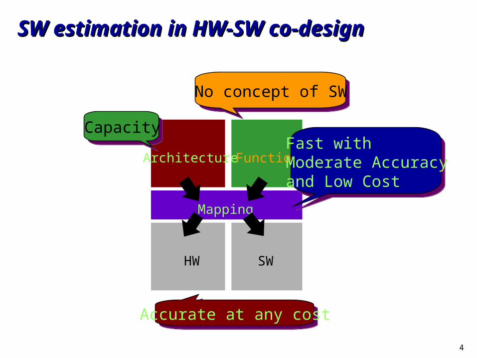
SW estimation in HW-SW co-designSW estimation in HW-SW co-design
Architecture Function
Mapping
HW SW
No concept of SW
Fast withModerate Accuracyand Low Cost
Accurate at any cost
Capacity
5
SW estimation overview: motivationSW estimation overview: motivation
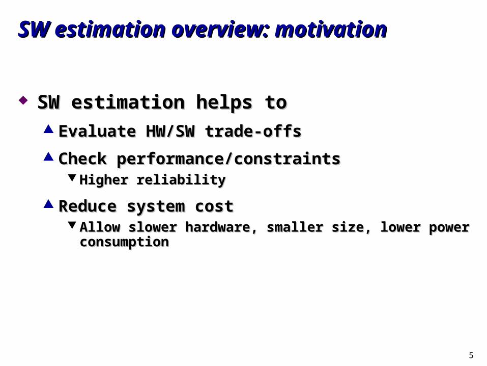
SW estimation helps toSW estimation helps to Evaluate HW/SW trade-offsEvaluate HW/SW trade-offs
Check performance/constraintsCheck performance/constraints Higher reliabilityHigher reliability
Reduce system costReduce system cost Allow slower hardware, smaller size, lower power consumptionAllow slower hardware, smaller size, lower power consumption
6
SW estimation overview: tasksSW estimation overview: tasks
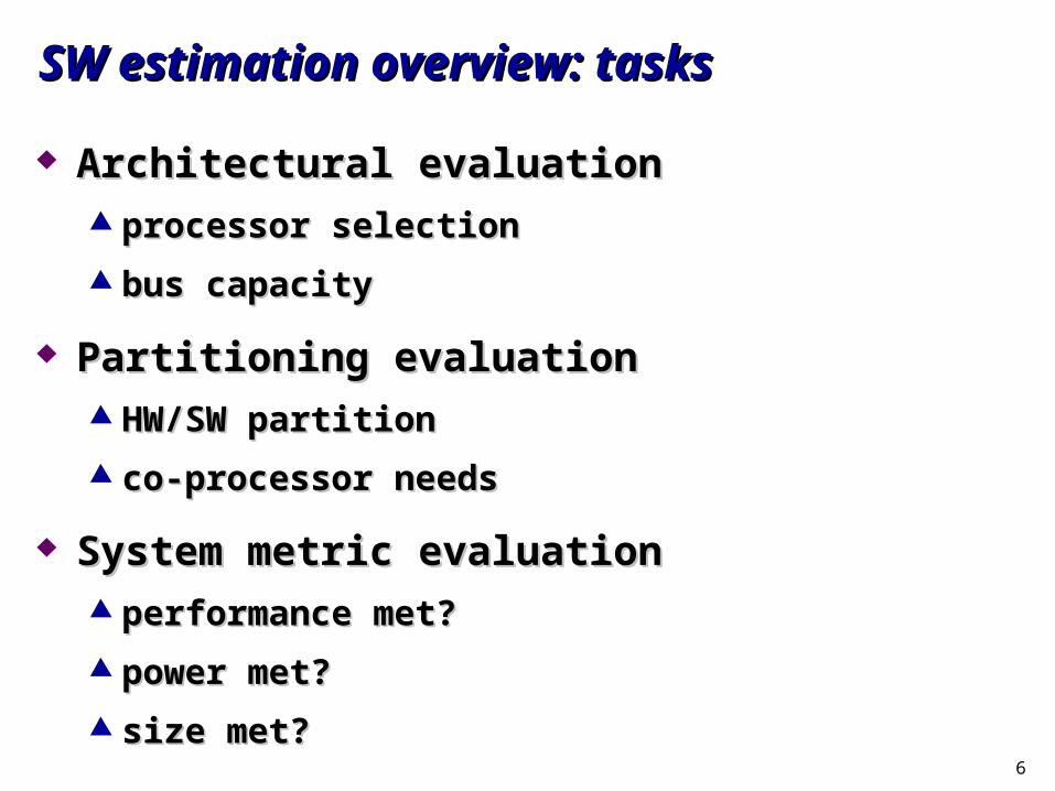
Architectural evaluationArchitectural evaluation processor selectionprocessor selection
bus capacitybus capacity
Partitioning evaluationPartitioning evaluation HW/SW partitionHW/SW partition
co-processor needsco-processor needs
System metric evaluationSystem metric evaluation performance met?performance met?
power met?power met?
size met?size met?
7
SW estimation overview: Static v.s. Dynamic SW estimation overview: Static v.s. Dynamic
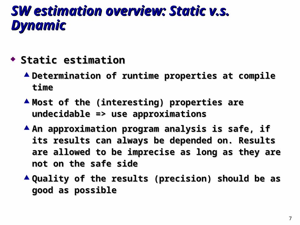
Static estimationStatic estimation Determination of runtime properties at compile timeDetermination of runtime properties at compile time
Most of the (interesting) properties are undecidable => use Most of the (interesting) properties are undecidable => use approximationsapproximations
An approximation program analysis is safe, if its results can An approximation program analysis is safe, if its results can always be depended on. Results are allowed to be imprecise as always be depended on. Results are allowed to be imprecise as long as they are not on the safe sidelong as they are not on the safe side
Quality of the results (precision) should be as good as possibleQuality of the results (precision) should be as good as possible
8
SW estimation overview: Static v.s. Dynamic SW estimation overview: Static v.s. Dynamic
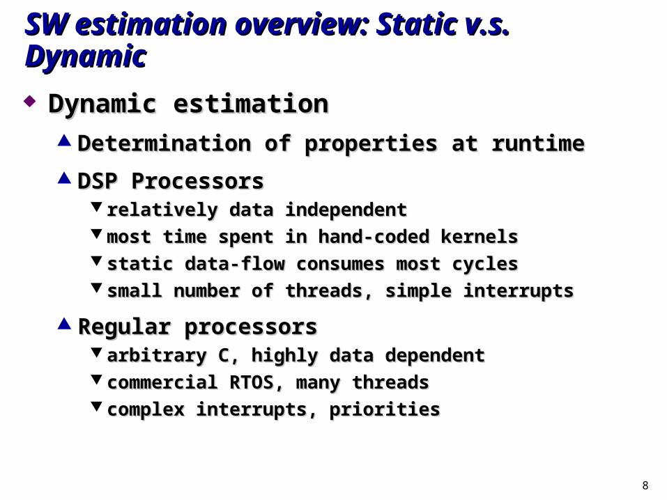
Dynamic estimationDynamic estimation Determination of properties at runtimeDetermination of properties at runtime
DSP ProcessorsDSP Processors relatively data independentrelatively data independent most time spent in hand-coded kernelsmost time spent in hand-coded kernels static data-flow consumes most cyclesstatic data-flow consumes most cycles small number of threads, simple interruptssmall number of threads, simple interrupts
Regular processorsRegular processors arbitrary C, highly data dependentarbitrary C, highly data dependent commercial RTOS, many threadscommercial RTOS, many threads complex interrupts, prioritiescomplex interrupts, priorities
9
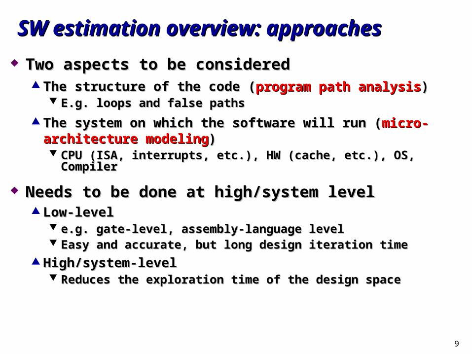
SW estimation overview: approachesSW estimation overview: approaches
Two aspects to be consideredTwo aspects to be considered The structure of the code (The structure of the code (program path analysisprogram path analysis))
E.g. loops and false pathsE.g. loops and false paths
The system on which the software will run (The system on which the software will run (micro-architecture modelingmicro-architecture modeling)) CPU (ISA, interrupts, etc.), HW (cache, etc.), OS, CompilerCPU (ISA, interrupts, etc.), HW (cache, etc.), OS, Compiler
Needs to be done at high/system levelNeeds to be done at high/system level Low-levelLow-level
e.g. gate-level, assembly-language levele.g. gate-level, assembly-language level Easy and accurate, but long design iteration timeEasy and accurate, but long design iteration time
High/system-levelHigh/system-level Reduces the exploration time of the design spaceReduces the exploration time of the design space
10
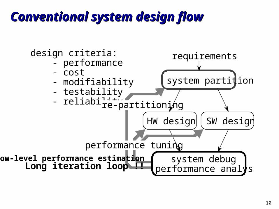
Conventional system design flowConventional system design flow
system partition
design criteria: - performance - cost - modifiability - testability - reliability
HW design SW design
requirements
re-partitioning
performance tuning
system debug performance analysisLong iteration loop !!
Low-level performance estimation
11
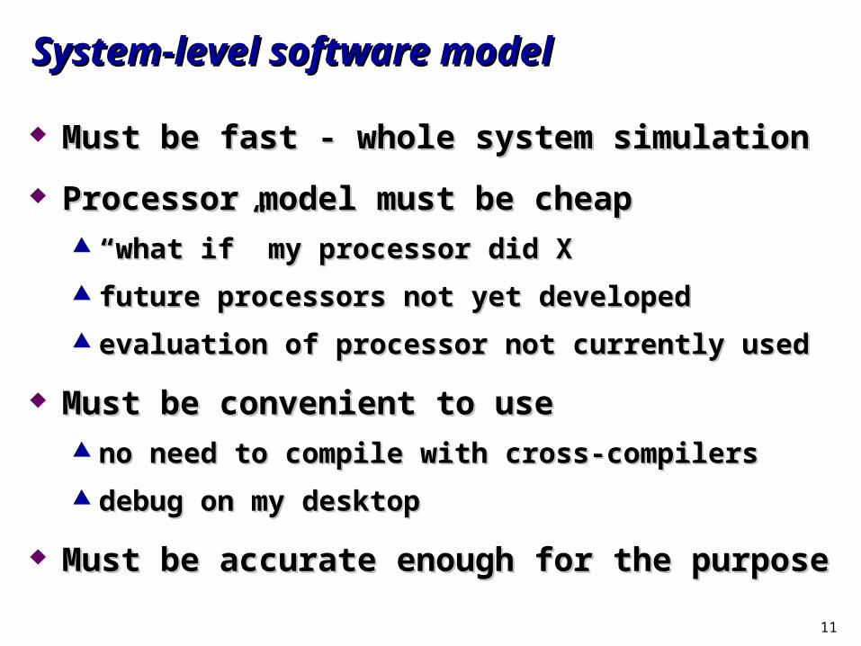
System-level software modelSystem-level software model
Must be fast - whole system simulationMust be fast - whole system simulation
Processor model must be cheapProcessor model must be cheap ““what if” my processor did Xwhat if” my processor did X
future processors not yet developedfuture processors not yet developed
evaluation of processor not currently usedevaluation of processor not currently used
Must be convenient to useMust be convenient to use no need to compile with cross-compilersno need to compile with cross-compilers
debug on my desktopdebug on my desktop
Must be accurate enough for the purposeMust be accurate enough for the purpose
12
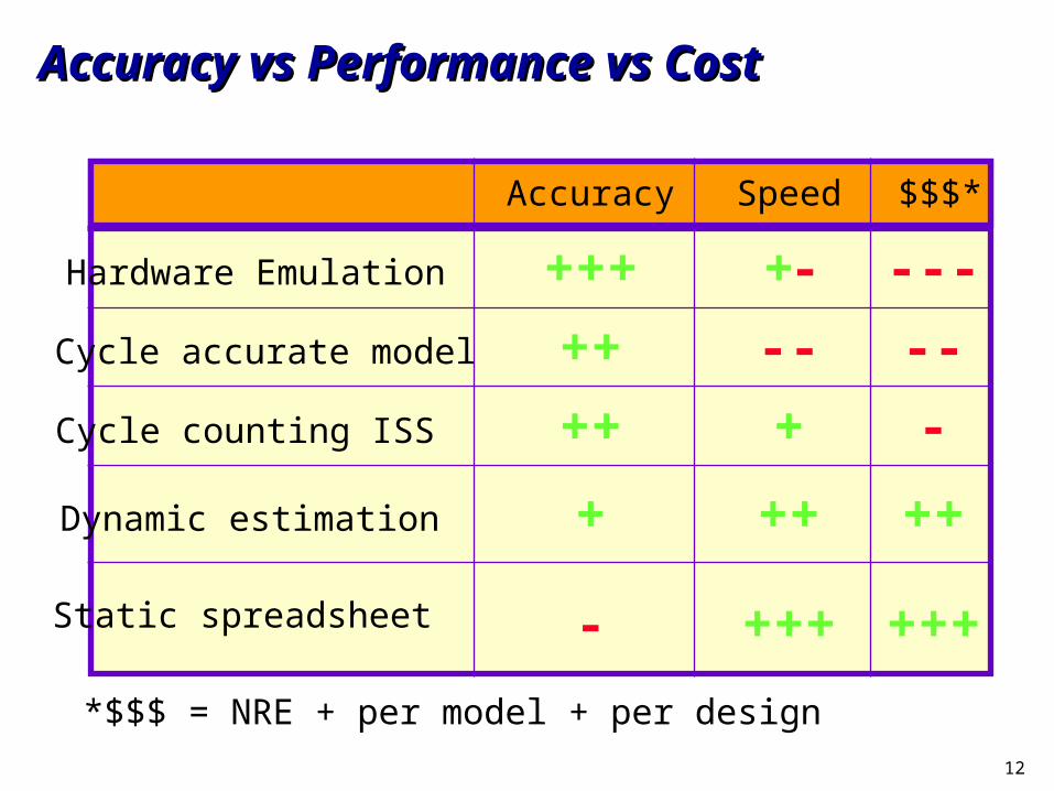
Accuracy vs Performance vs CostAccuracy vs Performance vs Cost
Hardware Emulation
Cycle accurate model
Cycle counting ISS
Static spreadsheet
Dynamic estimation
Accuracy Speed $$$*
+++ ---
--
+-
++ --
++ + -
+
-
++ ++
+++ +++
*$$$ = NRE + per model + per design
13
OutlineOutline
SW estimation overviewSW estimation overview
Program path analysisProgram path analysis
Micro-architecture modelingMicro-architecture modeling
Implementation examples: CinderellaImplementation examples: Cinderella
SW estimation in VCCSW estimation in VCC
SW estimation in AISW estimation in AI
SW estimation in POLISSW estimation in POLIS
14
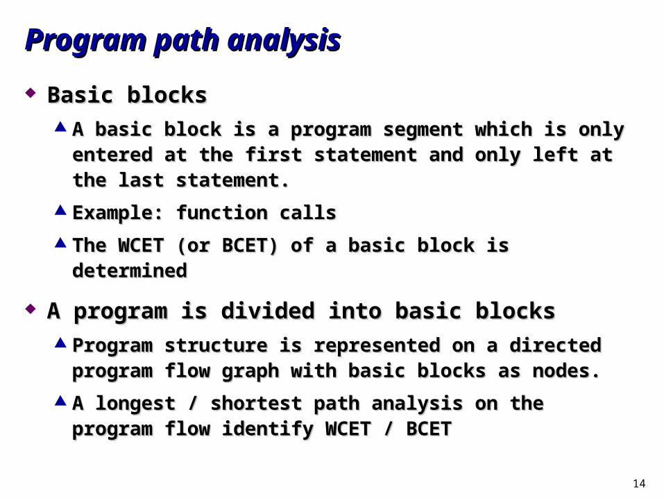
Program path analysisProgram path analysis
Basic blocksBasic blocks A basic block is a program segment which is only entered at the A basic block is a program segment which is only entered at the
first statement and only left at the last statement.first statement and only left at the last statement.
Example: function callsExample: function calls
The WCET (or BCET) of a basic block is determinedThe WCET (or BCET) of a basic block is determined
A program is divided into basic blocksA program is divided into basic blocks Program structure is represented on a directed program flow Program structure is represented on a directed program flow
graph with basic blocks as nodes.graph with basic blocks as nodes.
A longest / shortest path analysis on the program flow identify A longest / shortest path analysis on the program flow identify WCET / BCETWCET / BCET
15
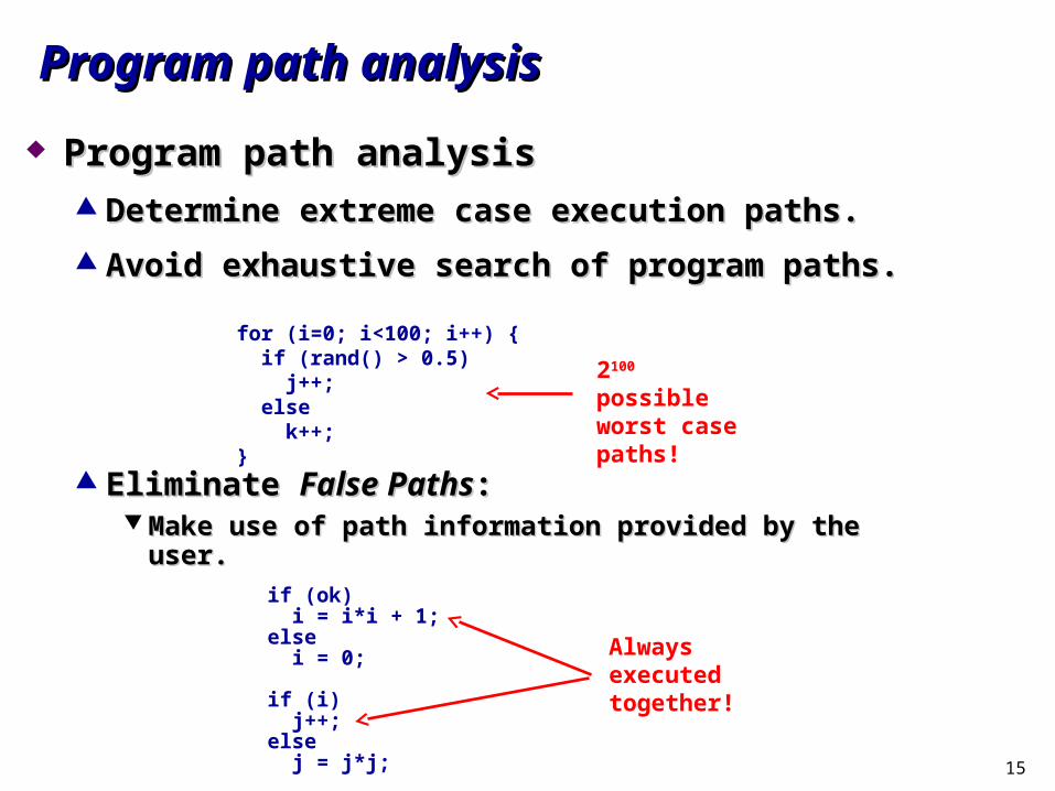
Program path analysisProgram path analysis
Program path analysisProgram path analysis Determine extreme case execution paths.Determine extreme case execution paths.
Avoid exhaustive search of program paths.Avoid exhaustive search of program paths.
Eliminate Eliminate False PathsFalse Paths:: Make use of path information provided by the user.Make use of path information provided by the user.
if (ok) i = i*i + 1;else i = 0;
if (i) j++;else j = j*j;
for (i=0; i<100; i++) { if (rand() > 0.5) j++; else k++;}
2100 possible worst case paths!
Always executed together!
16
Program path analysisProgram path analysis
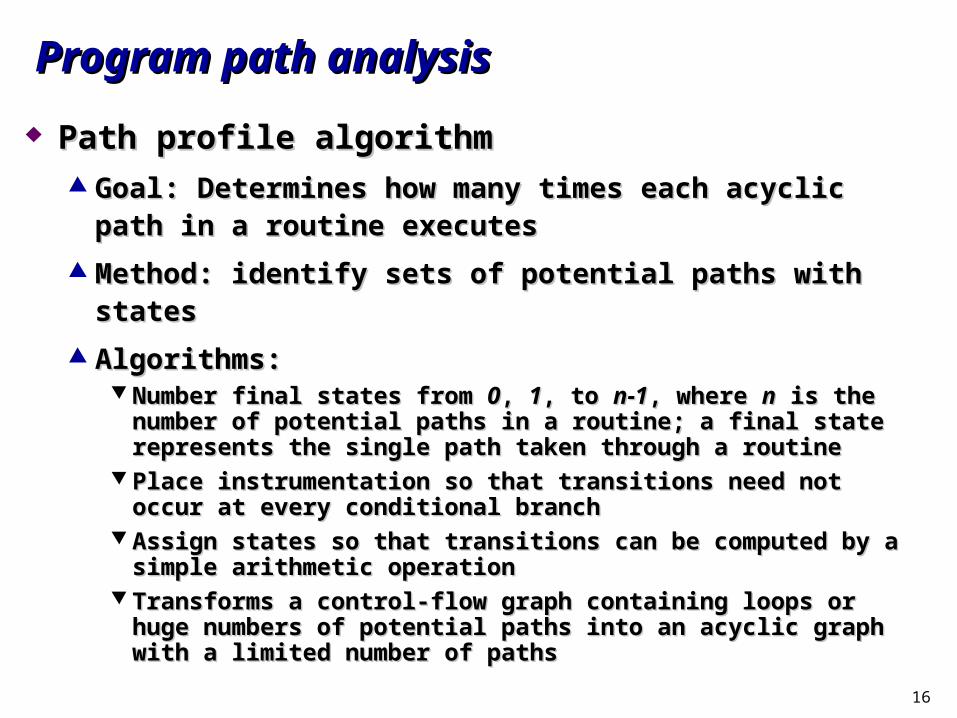
Path profile algorithmPath profile algorithm Goal: Determines how many times each acyclic path in a routine Goal: Determines how many times each acyclic path in a routine
executesexecutes
Method: identify sets of potential paths with statesMethod: identify sets of potential paths with states
Algorithms:Algorithms: Number final states from Number final states from 00, , 11, to , to n-1n-1, where , where nn is the number of potential is the number of potential
paths in a routine; a final state represents the single path taken through paths in a routine; a final state represents the single path taken through a routinea routine
Place instrumentation so that transitions need not occur at every Place instrumentation so that transitions need not occur at every conditional branchconditional branch
Assign states so that transitions can be computed by a simple arithmetic Assign states so that transitions can be computed by a simple arithmetic operationoperation
Transforms a control-flow graph containing loops or huge numbers of Transforms a control-flow graph containing loops or huge numbers of potential paths into an acyclic graph with a limited number of paths potential paths into an acyclic graph with a limited number of paths
17
Program path analysisProgram path analysis
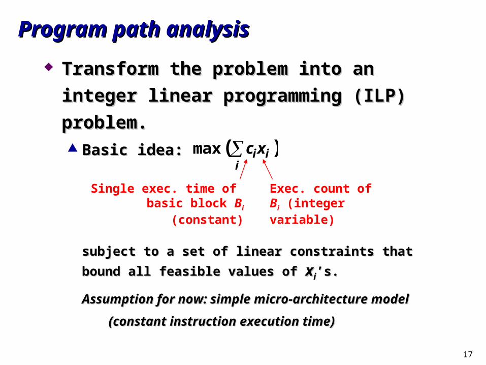
Transform the problem into an integer linear Transform the problem into an integer linear
programming (ILP) problem.programming (ILP) problem. Basic idea:Basic idea:
subject to a set of linear constraints that bound all feasible subject to a set of linear constraints that bound all feasible
values of values of xxii’s.’s.
Assumption for now: simple micro-architecture modelAssumption for now: simple micro-architecture model
(constant instruction execution (constant instruction execution time)time)
Exec. count of Bi (integer variable)
Single exec. time of basic block Bi (constant)
max( cixii )
18
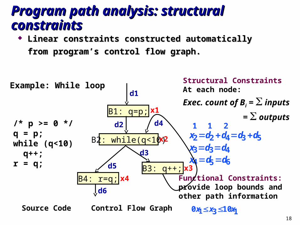
Program path analysis: structural constraintsProgram path analysis: structural constraints
Linear constraints constructed automatically from Linear constraints constructed automatically from
program’s control flow graph.program’s control flow graph.
Example: While loop
/* p >= 0 */q = p; while (q<10) q++;r = q;
Structural ConstraintsAt each node:
Exec. count of Bi = inputs
= outputs
Functional Constraints:provide loop bounds andother path information
Control Flow Graph
1 1 2x2d2 d4d3 d5x3d3d4x4d5d6
0x1x310x1Source Code
B1: q=p;
B4: r=q;
B2: while(q<10)
B3: q++;
d1
d2
d3
d5
d4
d6
x1
x2
x3x4
19
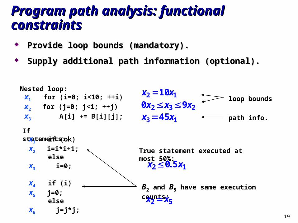
Program path analysis: functional constraintsProgram path analysis: functional constraints
Provide loop bounds (mandatory).Provide loop bounds (mandatory).
Supply additional path information (optional).Supply additional path information (optional).
x1 for (i=0; i<10; ++i)
x2 for (j=0; j<i; ++j)
x3 A[i] += B[i][j];
Nested loop:
loop bounds
path info.
If statements:x1 if (ok)
x2 i=i*i+1; else
x3 i=0;
x4 if (i)
x5 j=0; else
x6 j=j*j;
True statement executed at most 50%:
B2 and B5 have same execution counts:
x2 0.5x1
x2 x5
x2 10x1
0x2 x3 9x2
x3 45x1
20
OutlineOutline
SW estimation overviewSW estimation overview
Program path analysisProgram path analysis
Micro-architecture modelingMicro-architecture modeling
Implementation examples: CinderellaImplementation examples: Cinderella
SW estimation in VCCSW estimation in VCC
SW estimation in AISW estimation in AI
SW estimation in POLISSW estimation in POLIS
21
Micro-architecture modelingMicro-architecture modeling
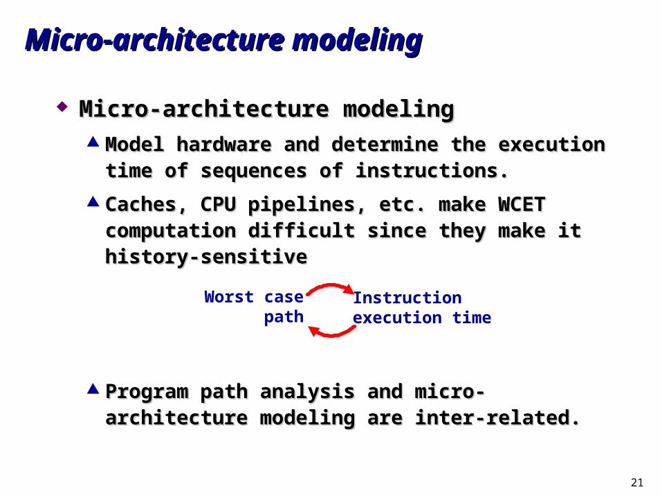
Micro-architecture modelingMicro-architecture modeling Model hardware and determine the execution time of Model hardware and determine the execution time of
sequences of instructions.sequences of instructions.
Caches, CPU pipelines, etc. make WCET computation Caches, CPU pipelines, etc. make WCET computation difficult since they make it history-sensitivedifficult since they make it history-sensitive
Program path analysis and micro-architecture modeling Program path analysis and micro-architecture modeling are inter-related.are inter-related.
Worst casepath
Instructionexecution time
22
Micro-architecture modelingMicro-architecture modeling
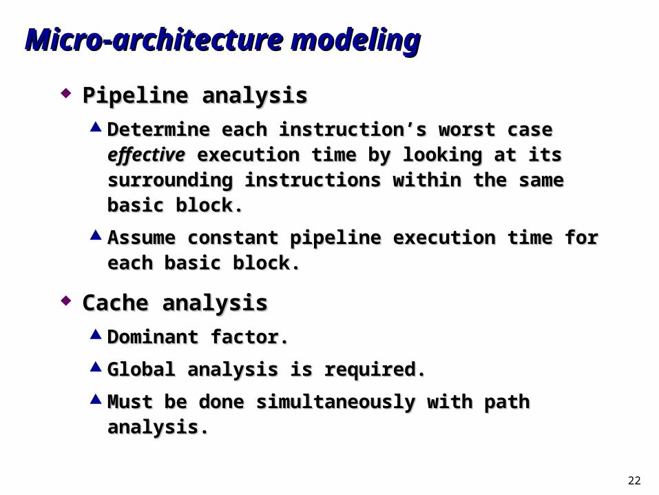
Pipeline analysisPipeline analysis Determine each instruction’s worst case Determine each instruction’s worst case effectiveeffective
execution time by looking at its surrounding instructions execution time by looking at its surrounding instructions within the same basic block.within the same basic block.
Assume constant pipeline execution time for each basic Assume constant pipeline execution time for each basic block.block.
Cache analysisCache analysis Dominant factor.Dominant factor.
Global analysis is required.Global analysis is required.
Must be done simultaneously with path analysis.Must be done simultaneously with path analysis.
23
Micro-architecture modelingMicro-architecture modeling
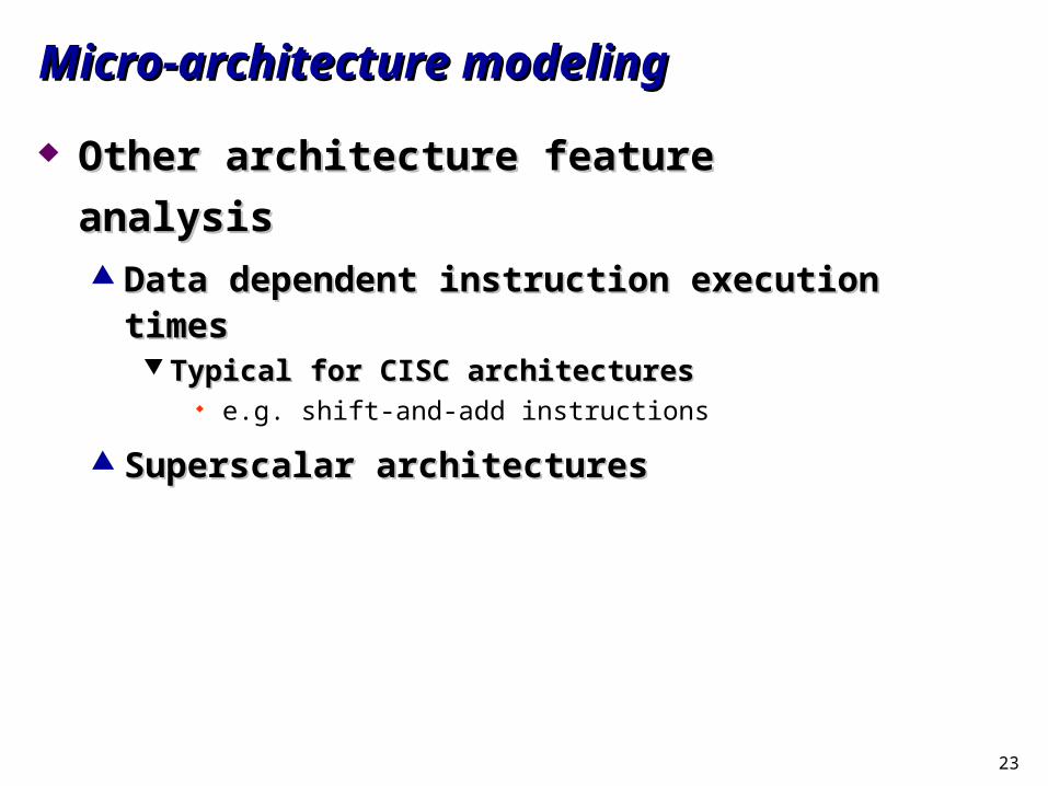
Other architecture feature analysisOther architecture feature analysis Data dependent instruction execution timesData dependent instruction execution times
Typical for CISC architecturesTypical for CISC architectures e.g. shift-and-add instructions
Superscalar architecturesSuperscalar architectures
24
Micro-architecture modeling: pipeline featuresMicro-architecture modeling: pipeline features
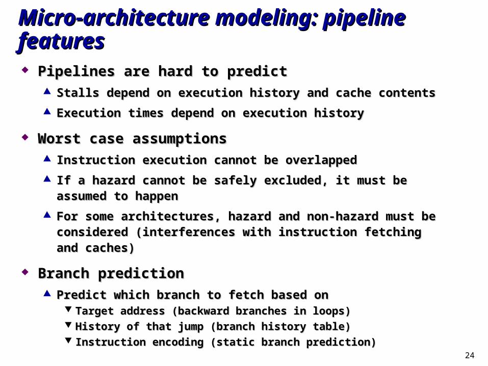
Pipelines are hard to predictPipelines are hard to predict Stalls depend on execution history and cache contentsStalls depend on execution history and cache contents
Execution times depend on execution historyExecution times depend on execution history
Worst case assumptionsWorst case assumptions Instruction execution cannot be overlappedInstruction execution cannot be overlapped
If a hazard cannot be safely excluded, it must be assumed to happenIf a hazard cannot be safely excluded, it must be assumed to happen
For some architectures, hazard and non-hazard must be considered For some architectures, hazard and non-hazard must be considered (interferences with instruction fetching and caches)(interferences with instruction fetching and caches)
Branch predictionBranch prediction Predict which branch to fetch based onPredict which branch to fetch based on
Target address (backward branches in loops)Target address (backward branches in loops) History of that jump (branch history table)History of that jump (branch history table) Instruction encoding (static branch prediction)Instruction encoding (static branch prediction)
25
Micro-architecture modeling: pipeline featuresMicro-architecture modeling: pipeline features
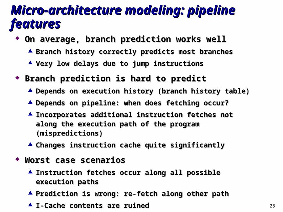
On average, branch prediction works wellOn average, branch prediction works well Branch history correctly predicts most branchesBranch history correctly predicts most branches
Very low delays due to jump instructionsVery low delays due to jump instructions
Branch prediction is hard to predictBranch prediction is hard to predict Depends on execution history (branch history table)Depends on execution history (branch history table)
Depends on pipeline: when does fetching occur?Depends on pipeline: when does fetching occur?
Incorporates additional instruction fetches not along the execution Incorporates additional instruction fetches not along the execution path of the program (mispredictions)path of the program (mispredictions)
Changes instruction cache quite significantlyChanges instruction cache quite significantly
Worst case scenariosWorst case scenarios Instruction fetches occur along all possible execution pathsInstruction fetches occur along all possible execution paths
Prediction is wrong: re-fetch along other pathPrediction is wrong: re-fetch along other path
I-Cache contents are ruinedI-Cache contents are ruined
26
Micro-architecture modeling: pipeline analysisMicro-architecture modeling: pipeline analysis
Goal: calculate all possible pipeline states at a program pointGoal: calculate all possible pipeline states at a program point
Method: perform a cycle-wise evolution of the pipeline, determining all Method: perform a cycle-wise evolution of the pipeline, determining all
possible successor pipeline statespossible successor pipeline states
Implemented from a formal model of the pipeline, its stages and Implemented from a formal model of the pipeline, its stages and
communication between themcommunication between them
Generated from a PAG specificationGenerated from a PAG specification
Results in WCET for basic blocksResults in WCET for basic blocks
Abstract state is a set of concrete pipeline states; try to obtain a superset Abstract state is a set of concrete pipeline states; try to obtain a superset
of the collecting semanticsof the collecting semantics
Sets are small as pipeline is not too history-sensitiveSets are small as pipeline is not too history-sensitive
Joins in CFG are set unionJoins in CFG are set union
27
Micro-architecture modeling: I-cache analysisMicro-architecture modeling: I-cache analysis
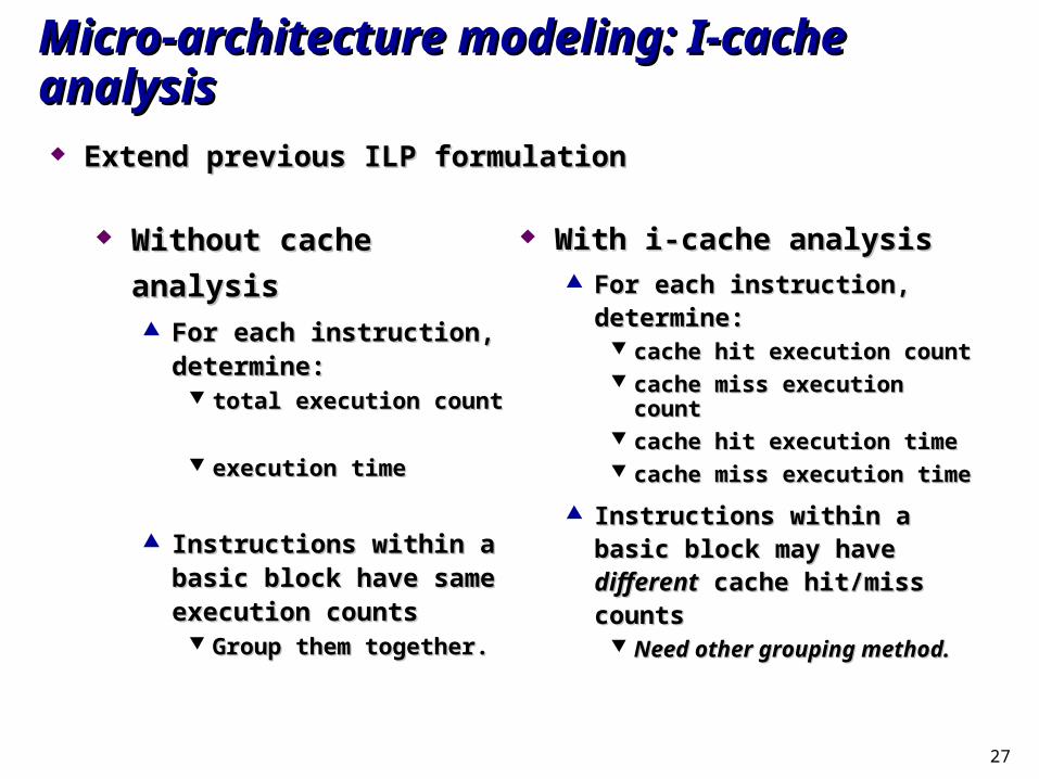
Without cache analysisWithout cache analysis For each instruction, For each instruction,
determine:determine: total execution counttotal execution count
execution timeexecution time
Instructions within a basic Instructions within a basic block have same execution block have same execution countscounts
Group them together.Group them together.
With i-cache analysisWith i-cache analysis For each instruction, determine:For each instruction, determine:
cache hit execution countcache hit execution count cache miss execution countcache miss execution count cache hit execution timecache hit execution time cache miss execution timecache miss execution time
Instructions within a basic block Instructions within a basic block may have may have differentdifferent cache cache hit/miss countshit/miss counts
Need other grouping method.Need other grouping method.
Extend previous ILP formulationExtend previous ILP formulation
28
Grouping Instructions: Line-blocksGrouping Instructions: Line-blocks
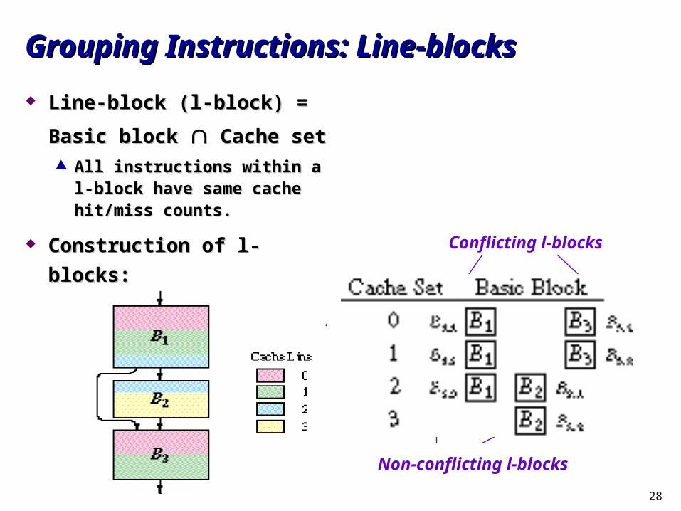
Line-block (l-block) = Basic Line-block (l-block) = Basic
block block Cache set Cache set All instructions within a l-block All instructions within a l-block
have same cache hit/miss have same cache hit/miss counts.counts.
Construction of l-blocks:Construction of l-blocks:Conflicting l-blocks
Non-conflicting l-blocks
29
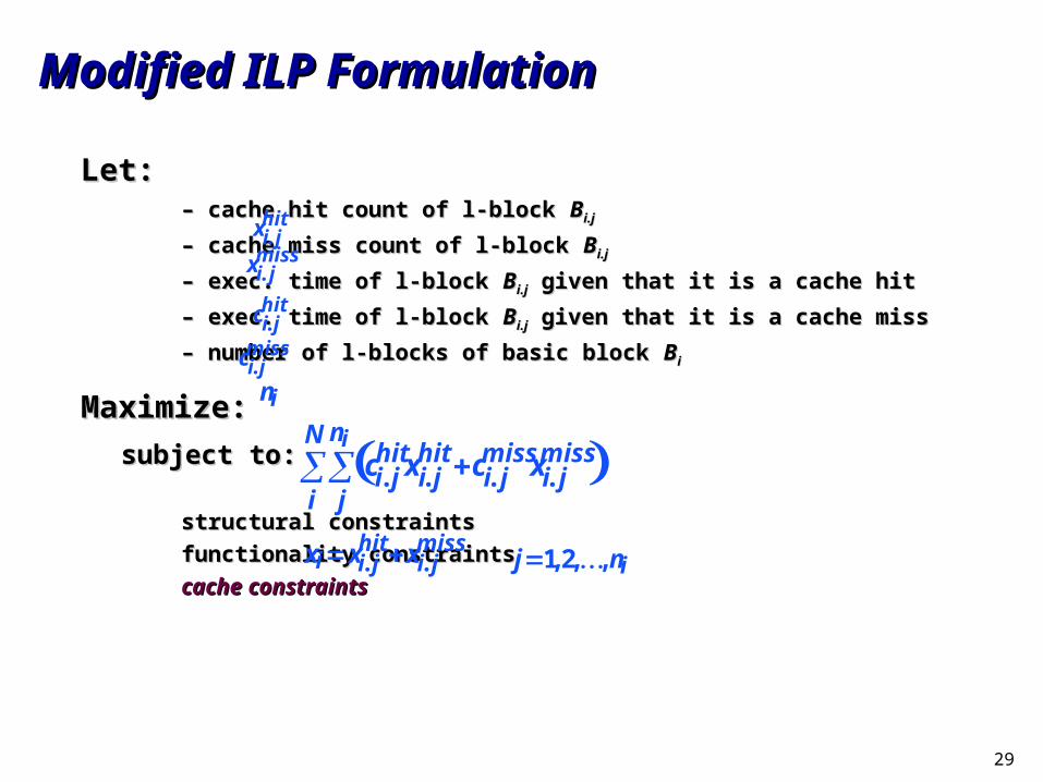
Modified ILP FormulationModified ILP Formulation
Let:Let:– – cache hit count of l-block cache hit count of l-block BBi.ji.j
– – cache miss count of l-block cache miss count of l-block BBi.ji.j
– – exec. time of l-block exec. time of l-block BBi.ji.j given that it is a cache hit given that it is a cache hit
– – exec. time of l-block exec. time of l-block BBi.ji.j given that it is a cache miss given that it is a cache miss
– – number of l-blocks of basic block number of l-blocks of basic block BBii
Maximize:Maximize:
subject to:subject to:
structural constraintsstructural constraints
functionality constraintsfunctionality constraints
cache constraintscache constraints
ci.jhitxi.j
hitci. jmissxi. j
miss j
ni
i
N
xi. jhit
xi. jmiss
ci.jhit
ci.jmiss
xixi.jhitxi. j
missj1,2,,ni
ni
30
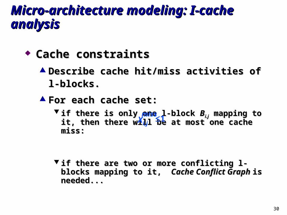
Micro-architecture modeling: I-cache analysisMicro-architecture modeling: I-cache analysis
Cache constraintsCache constraints Describe cache hit/miss activities of l-blocks.Describe cache hit/miss activities of l-blocks.
For each cache set:For each cache set: if there is only one l-block if there is only one l-block BBi.ji.j mapping to it, then there will be at mapping to it, then there will be at
most one cache miss:most one cache miss:
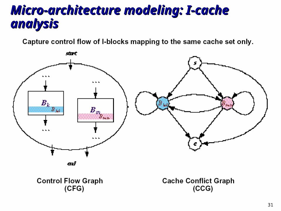
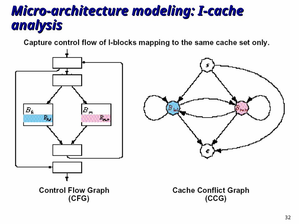
if there are two or more conflicting l-blocks mapping to it, if there are two or more conflicting l-blocks mapping to it, Cache Conflict Graph Cache Conflict Graph is needed...is needed...
Xi,j
miss≤1
31
Micro-architecture modeling: I-cache analysisMicro-architecture modeling: I-cache analysis
32
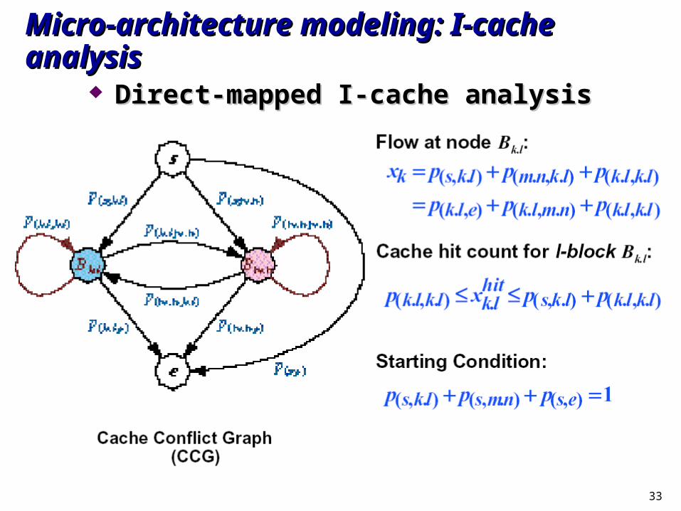
Micro-architecture modeling: I-cache analysisMicro-architecture modeling: I-cache analysis
33
Micro-architecture modeling: I-cache analysisMicro-architecture modeling: I-cache analysis
Direct-mapped I-cache analysisDirect-mapped I-cache analysis
34
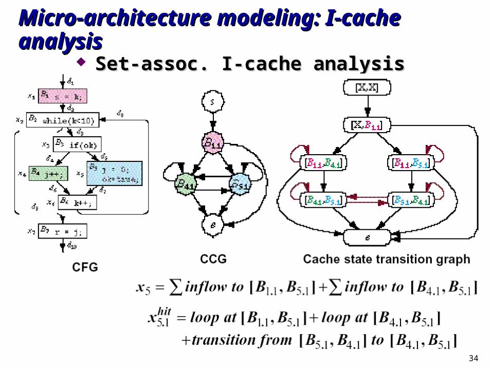
Micro-architecture modeling: I-cache analysisMicro-architecture modeling: I-cache analysis Set-assoc. I-cache analysisSet-assoc. I-cache analysis
35
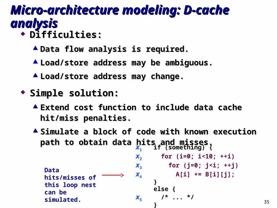
Micro-architecture modeling: D-cache analysisMicro-architecture modeling: D-cache analysis Difficulties:Difficulties:
Data flow analysis is required.Data flow analysis is required.
Load/store address may be ambiguous.Load/store address may be ambiguous.
Load/store address may change.Load/store address may change.
Simple solution:Simple solution: Extend cost function to include data cache hit/miss penalties.Extend cost function to include data cache hit/miss penalties.
Simulate a block of code with known execution path to obtain Simulate a block of code with known execution path to obtain data hits and misses.data hits and misses. x1 if (something) {
x2 for (i=0; i<10; ++i)
x3 for (j=0; j<i; ++j)
x4 A[i] += B[i][j]; } else {
x5 /* ... */ }
Data hits/misses of this loop nest can be simulated.
36
OutlineOutline
SW estimation overviewSW estimation overview
Program path analysisProgram path analysis
Micro-architecture modelingMicro-architecture modeling
Implementation examples: CinderellaImplementation examples: Cinderella
SW estimation in VCCSW estimation in VCC
SW estimation in AISW estimation in AI
SW estimation in POLISSW estimation in POLIS
37
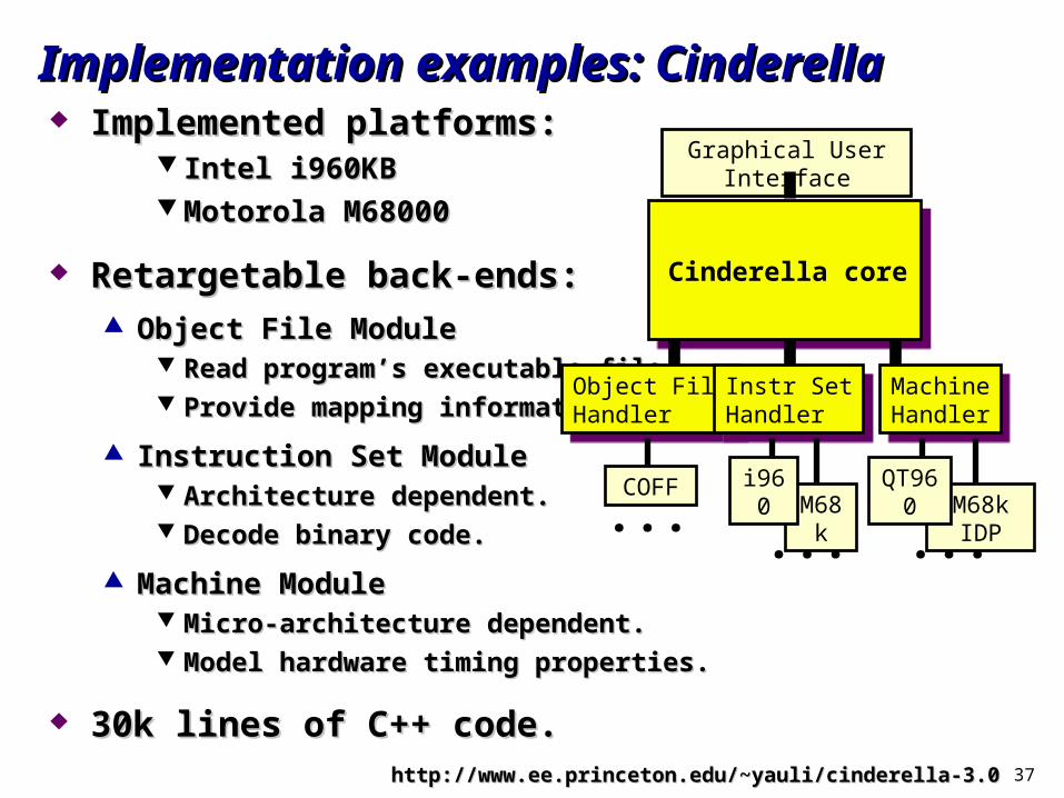
Implementation examples: CinderellaImplementation examples: Cinderella Implemented platforms:Implemented platforms:
Intel i960KBIntel i960KB Motorola M68000Motorola M68000
Retargetable back-ends:Retargetable back-ends: Object File ModuleObject File Module
Read program’s executable file.Read program’s executable file. Provide mapping information.Provide mapping information.
Instruction Set ModuleInstruction Set Module Architecture dependent.Architecture dependent. Decode binary code.Decode binary code.
Machine ModuleMachine Module Micro-architecture dependent.Micro-architecture dependent. Model hardware timing properties.Model hardware timing properties.
30k lines of C++ code.30k lines of C++ code. http://www.ee.princeton.edu/~yauli/cinderella-3.0http://www.ee.princeton.edu/~yauli/cinderella-3.0
Cinderella core
...M68k IDP
QT960M6
8k ...
i960
COFF
Object FileHandler
Object FileHandler
Instr SetHandler
Instr SetHandler
...
MachineHandler
MachineHandler
Graphical User Interface
38
Implementation examples: CinderellaImplementation examples: Cinderella
Timing analysis is done at machine code level.Timing analysis is done at machine code level. read executable file directly.read executable file directly.
Annotation is done at source level.Annotation is done at source level. need to map machine code to source code.need to map machine code to source code.
use debugging information stored in executable file.use debugging information stored in executable file.
Advantages:Advantages: source level, compiler independent.source level, compiler independent. optimum code quality.optimum code quality.
Reduce retargeting efforts.Reduce retargeting efforts. Identify target dependent modules.Identify target dependent modules.
39
Implementation examples: CinderellaImplementation examples: Cinderella
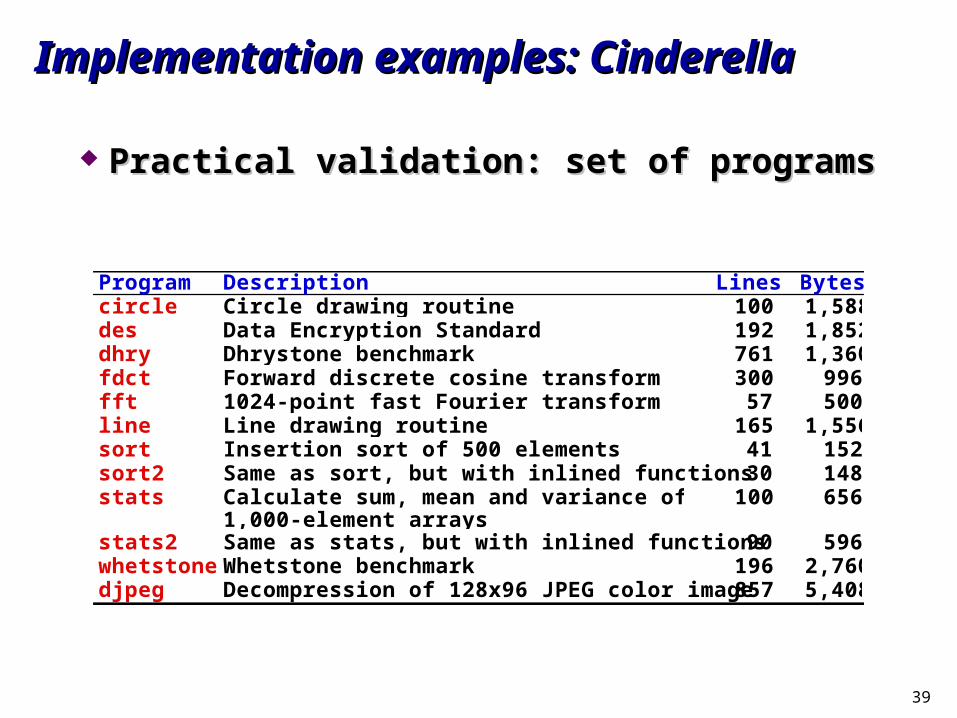
Practical validation: set of programsPractical validation: set of programs
Program Description Lines Bytescircle Circle drawing routine 100 1,588des Data Encryption Standard 192 1,852dhry Dhrystone benchmark 761 1,360fdct Forward discrete cosine transform 300 996fft 1024-point fast Fourier transform 57 500line Line drawing routine 165 1,556sort Insertion sort of 500 elements 41 152sort2 Same as sort, but with inlined functions 30 148stats Calculate sum, mean and variance of two
1,000-element arrays100 656
stats2 Same as stats, but with inlined functions 90 596whetstone Whetstone benchmark 196 2,760djpeg Decompression of 128x96 JPEG color image 857 5,408
40
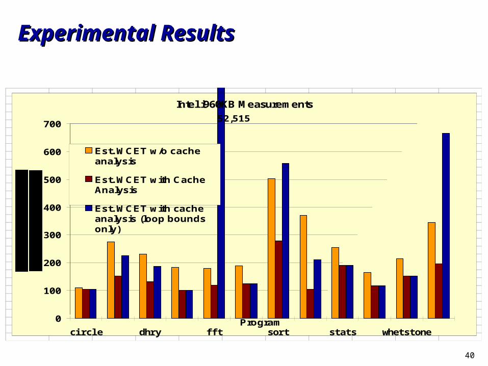
Experimental ResultsExperimental Results
Intel i960KB Measurements
0
100
200
300
400
500
600
700
circle dhry fft sort stats whetstoneProgram
Est. WCET w/o cacheanalysis
Est. WCET with CacheAnalysis
Est. WCET with cacheanalysis (loop boundsonly)
52,515
41
Implementation examples: CinderellaImplementation examples: Cinderella
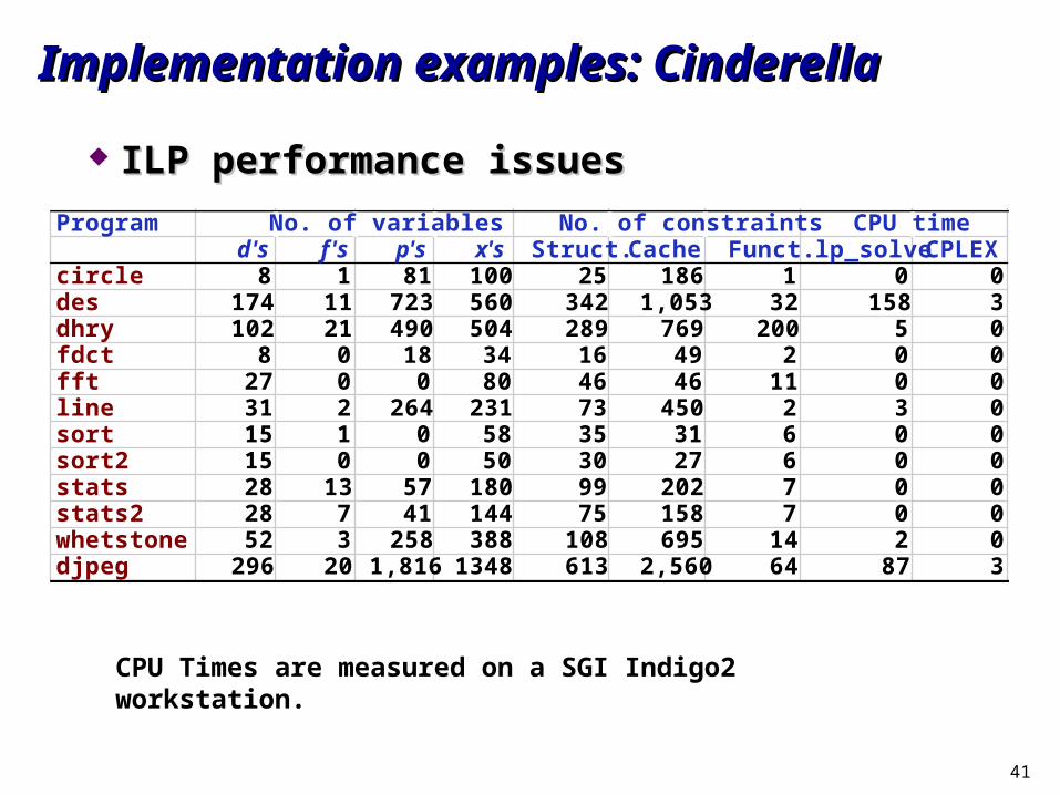
ILP performance issuesILP performance issues
Program No. of variables No. of constraints CPU timed's f's p's x's Struct. Cache Funct. lp_solve CPLEX
circle 8 1 81 100 25 186 1 0 0des 174 11 723 560 342 1,053 32 158 3dhry 102 21 490 504 289 769 200 5 0fdct 8 0 18 34 16 49 2 0 0fft 27 0 0 80 46 46 11 0 0line 31 2 264 231 73 450 2 3 0sort 15 1 0 58 35 31 6 0 0sort2 15 0 0 50 30 27 6 0 0stats 28 13 57 180 99 202 7 0 0stats2 28 7 41 144 75 158 7 0 0whetstone 52 3 258 388 108 695 14 2 0djpeg 296 20 1,816 1348 613 2,560 64 87 3
CPU Times are measured on a SGI Indigo2 workstation.
42
OutlineOutline
SW estimation overviewSW estimation overview
Program path analysisProgram path analysis
Micro-architecture modelingMicro-architecture modeling
Implementation examples: CinderellaImplementation examples: Cinderella
SW estimation in VCCSW estimation in VCC
SW estimation in AISW estimation in AI
SW estimation in POLISSW estimation in POLIS
43
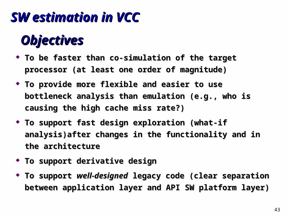
SW estimation in VCCSW estimation in VCC
To be faster than co-simulation of the target processor (at least To be faster than co-simulation of the target processor (at least
one order of magnitude)one order of magnitude)
To provide more flexible and easier to use bottleneck analysis To provide more flexible and easier to use bottleneck analysis
than emulation (e.g., who is causing the high cache miss rate?)than emulation (e.g., who is causing the high cache miss rate?)
To support fast design exploration (what-if analysis)after changes To support fast design exploration (what-if analysis)after changes
in the functionality and in the architecturein the functionality and in the architecture
To support derivative designTo support derivative design
To support To support well-designedwell-designed legacy code (clear separation between legacy code (clear separation between
application layer and API SW platform layer)application layer and API SW platform layer)
ObjectivesObjectives
44
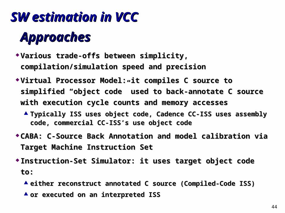
SW estimation in VCCSW estimation in VCC
ApproachesApproaches Various trade-offs between simplicity, compilation/simulation speed and Various trade-offs between simplicity, compilation/simulation speed and
precisionprecision
Virtual Processor Model: it compiles C source to simplified “object code” used Virtual Processor Model: it compiles C source to simplified “object code” used
to back-annotate C source with execution cycle counts and memory accessesto back-annotate C source with execution cycle counts and memory accesses Typically ISS uses object code, Cadence CC-ISS uses assembly code, commercial CC-Typically ISS uses object code, Cadence CC-ISS uses assembly code, commercial CC-
ISS’s use object codeISS’s use object code
CABA: C-Source Back Annotation and model calibration via Target Machine CABA: C-Source Back Annotation and model calibration via Target Machine
Instruction SetInstruction Set
Instruction-Set Simulator: it uses target object code to:Instruction-Set Simulator: it uses target object code to: either reconstruct annotated C source (Compiled-Code ISS)either reconstruct annotated C source (Compiled-Code ISS)
or executed on an interpreted ISSor executed on an interpreted ISS
45
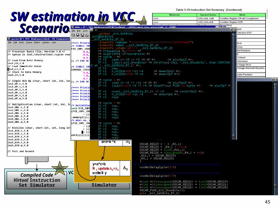
SW estimation in VCCSW estimation in VCCScenariosScenarios
Target Processor
VCC
White Box C
VCCVirtual
Compiler
Target Processor
Compiler
HostCompiler
Compiled CodeVirtual Instruction
Set Simulator
Compiled Code Instruction Set
Simulator
InterpretedInstruction Set
Simulator
TargetProcessorInstruction
Set
VCC Virtual
ProcessorInstruction
Set
.obj
AnnotatedWhite Box C
AnnotatedWhite Box C .obj
.obj
HostCompiler
Target Assembly Code
ASM 2 C
Compiled Code
Processor Model
Co-simulation
tmp=b+cc=f(d)MT update 1
1
y=a*c+bMT update 2+3
write B y3
f6(y)MT update 4
return4
r=(s<<*a)a=r+m*x 2
tmp !tmp
46
SW estimation in VCCSW estimation in VCC
LimitationsLimitations
C (or assembler) library routine estimation (e.g. C (or assembler) library routine estimation (e.g.
trigonometric functions): the delay should be part of the trigonometric functions): the delay should be part of the
library modellibrary model
Import of arbitrary (especially processor or RTOS-Import of arbitrary (especially processor or RTOS-
dependent) legacy codedependent) legacy code Code must adhere to the simulator interface including Code must adhere to the simulator interface including
embedded system calls (RTOS): the conversion is not the aim embedded system calls (RTOS): the conversion is not the aim of software estimationof software estimation
47
SW estimation in VCCSW estimation in VCCVirtual Processor Model (VPM)Virtual Processor Model (VPM)compiled code virtual instruction set simulatorcompiled code virtual instruction set simulator
Pros:Pros:does not require target software development chaindoes not require target software development chain
fast simulation model generation and executionfast simulation model generation and execution
simple and cheap generation of a new processor modelsimple and cheap generation of a new processor model
Needed when target processor and compiler not availableNeeded when target processor and compiler not available
Cons:Cons:hard to model target compiler optimizations (requires “best in hard to model target compiler optimizations (requires “best in
class” Virtual Compiler that can also as C-to-C optimization for class” Virtual Compiler that can also as C-to-C optimization for the target compiler)the target compiler)
low precision, especially for data memory accesseslow precision, especially for data memory accesses
48
SW estimation in VCCSW estimation in VCC
Interpreted instruction set simulator (I-ISS)Interpreted instruction set simulator (I-ISS)Pros:Pros:
generally available from processor IP providergenerally available from processor IP provider
often integrates fast cache modeloften integrates fast cache model
considers target compiler optimizations and real data and code addressesconsiders target compiler optimizations and real data and code addresses
Cons: Cons: requires target software development chainrequires target software development chain
often low speedoften low speed
different integration problem for every vendor (and often for every CPU)different integration problem for every vendor (and often for every CPU)
may be difficult to support communication models that require waiting to may be difficult to support communication models that require waiting to complete an I/O or synchronization operationcomplete an I/O or synchronization operation
49
SW estimation in VCCSW estimation in VCC
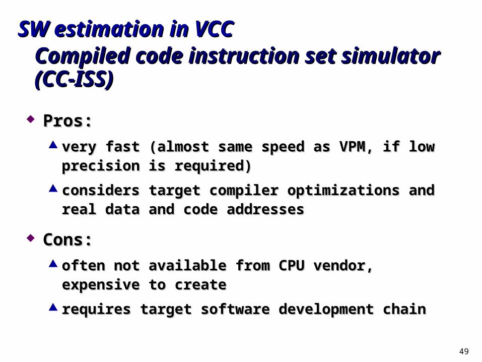
Compiled code instruction set simulator (CC-ISS)Compiled code instruction set simulator (CC-ISS)
Pros:Pros: very fast (almost same speed as VPM, if low precision is very fast (almost same speed as VPM, if low precision is
required)required)
considers target compiler optimizations and real data and considers target compiler optimizations and real data and code addressescode addresses
Cons:Cons: often not available from CPU vendor, expensive to createoften not available from CPU vendor, expensive to create
requires target software development chainrequires target software development chain
50
SW estimation in VCCSW estimation in VCC
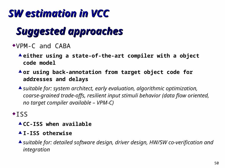
Suggested approachesSuggested approachesVPM-C and CABA
either using a state-of-the-art compiler with a object code model
or using back-annotation from target object code for addresses and delays
suitable for: system architect, early evaluation, algorithmic optimization, coarse-grained trade-offs, resilient input stimuli behavior (data flow oriented, no target compiler available – VPM-C)
ISS CC-ISS when available
I-ISS otherwise
suitable for: detailed software design, driver design, HW/SW co-verification and integration
51
SW estimation in VCCSW estimation in VCC
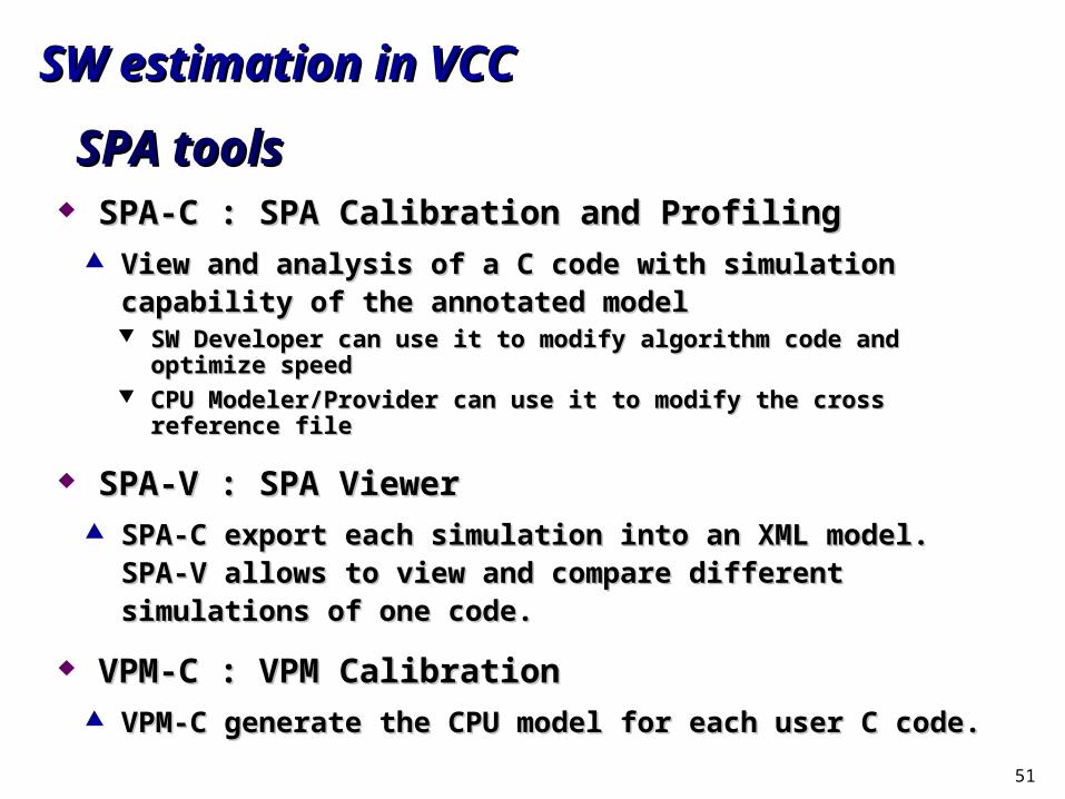
SPA toolsSPA tools SPA-C : SPA Calibration and ProfilingSPA-C : SPA Calibration and Profiling
View and analysis of a C code with simulation capability of the View and analysis of a C code with simulation capability of the annotated modelannotated model SW Developer can use it to modify algorithm code and optimize speed SW Developer can use it to modify algorithm code and optimize speed CPU Modeler/Provider can use it to modify the cross reference fileCPU Modeler/Provider can use it to modify the cross reference file
SPA-V : SPA ViewerSPA-V : SPA Viewer SPA-C export each simulation into an XML model. SPA-V SPA-C export each simulation into an XML model. SPA-V
allows to view and compare different simulations of one code.allows to view and compare different simulations of one code.
VPM-C : VPM CalibrationVPM-C : VPM Calibration VPM-C generate the CPU model for each user C code.VPM-C generate the CPU model for each user C code.

52
SW estimation in VCCSW estimation in VCCSPA tool chainSPA tool chain
Can startsSPA-C
Automatically
SPA Viewer
SPA Calibration
Can startsVPM-C
Automatically
VPM Calibration (FIRST)
53
SW estimation in VCCSW estimation in VCC
VPM-C: goalsVPM-C: goals
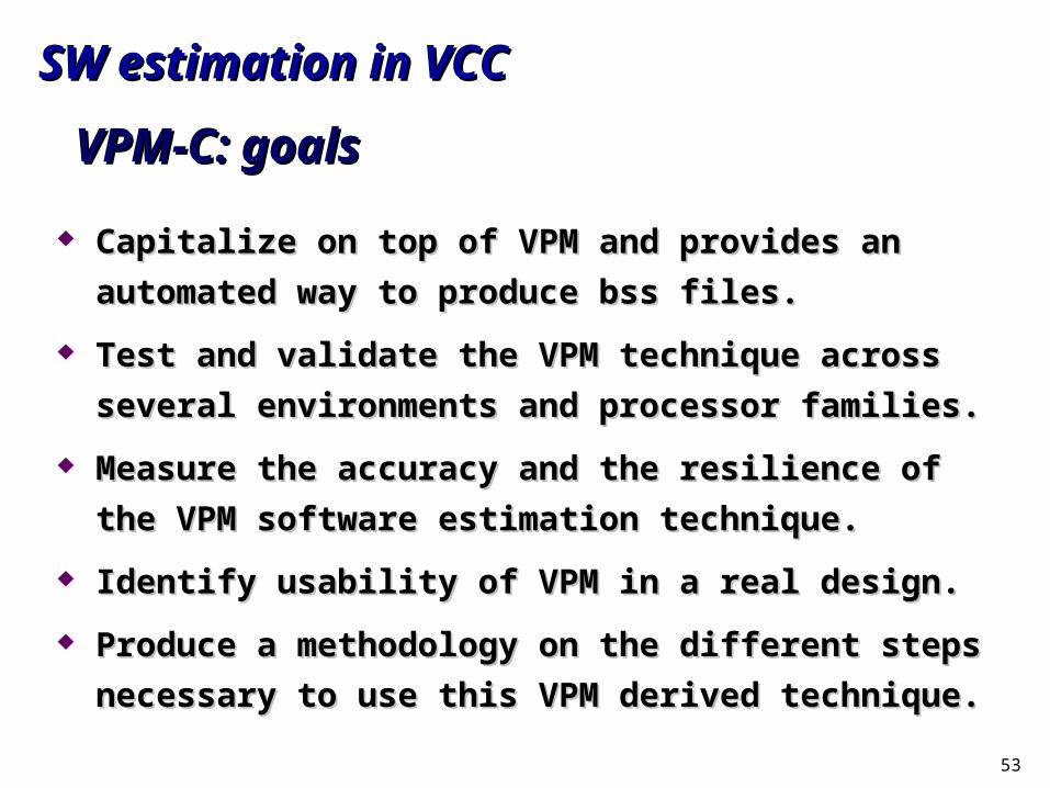
Capitalize on top of VPM and provides an automated way to Capitalize on top of VPM and provides an automated way to
produce bss files.produce bss files.
Test and validate the VPM technique across several Test and validate the VPM technique across several
environments and processor families.environments and processor families.
Measure the accuracy and the resilience of the VPM software Measure the accuracy and the resilience of the VPM software
estimation technique.estimation technique.
Identify usability of VPM in a real design.Identify usability of VPM in a real design.
Produce a methodology on the different steps necessary to use Produce a methodology on the different steps necessary to use
this VPM derived technique.this VPM derived technique.
54
SW estimation in VCCSW estimation in VCC
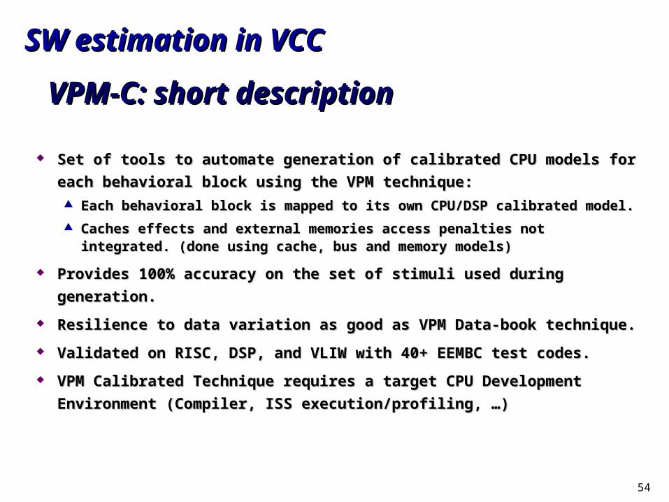
VPM-C: short descriptionVPM-C: short description
Set of tools to automate generation of calibrated CPU models for each Set of tools to automate generation of calibrated CPU models for each
behavioral block using the VPM technique:behavioral block using the VPM technique: Each behavioral block is mapped to its own CPU/DSP calibrated model.Each behavioral block is mapped to its own CPU/DSP calibrated model.
Caches effects and external memories access penalties not integrated. (done using Caches effects and external memories access penalties not integrated. (done using cache, bus and memory models)cache, bus and memory models)
Provides 100% accuracy on the set of stimuli used during generation.Provides 100% accuracy on the set of stimuli used during generation.
Resilience to data variation as good as VPM Data-book technique.Resilience to data variation as good as VPM Data-book technique.
Validated on RISC, DSP, and VLIW with 40+ EEMBC test codes.Validated on RISC, DSP, and VLIW with 40+ EEMBC test codes.
VPM Calibrated Technique requires a target CPU Development Environment VPM Calibrated Technique requires a target CPU Development Environment
(Compiler, ISS execution/profiling, …)(Compiler, ISS execution/profiling, …)
55
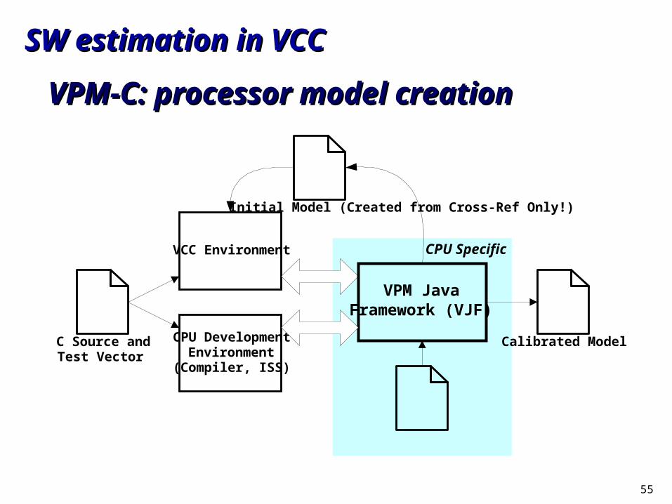
SW estimation in VCCSW estimation in VCC
VPM-C: processor model creationVPM-C: processor model creation
C Source andTest Vector
Initial Model (Created from Cross-Ref Only!)
CPU DevelopmentEnvironment
(Compiler, ISS)
VCC Environment
Calibrated Model
VPM JavaFramework (VJF)
CPU Specific
56
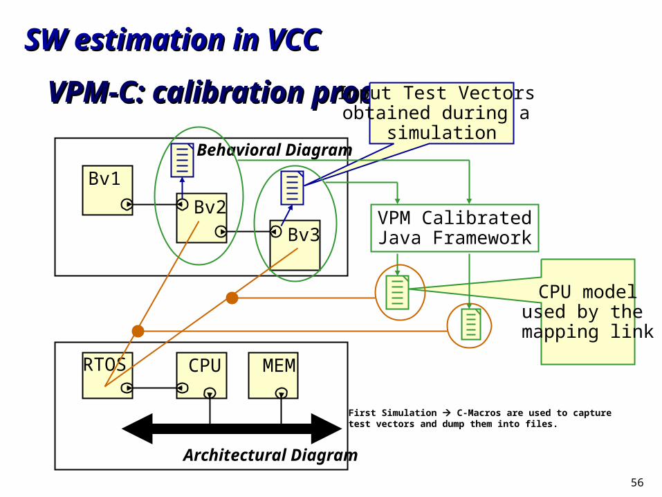
SW estimation in VCCSW estimation in VCC
VPM-C: calibration processVPM-C: calibration process
RTOS CPU MEM
Architectural Diagram
Bv1
Bv2Bv3
Behavioral Diagram
Input Test Vectors obtained during a
simulation
VPM CalibratedJava Framework
CPU modelused by the mapping link
First Simulation C-Macros are used to capture test vectors and dump them into files.
57
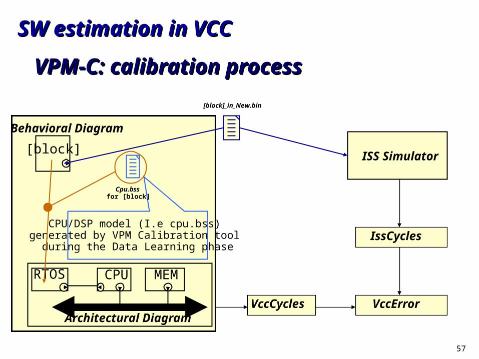
SW estimation in VCCSW estimation in VCC
VPM-C: calibration processVPM-C: calibration process
RTOS CPU MEM
Architectural Diagram
[block]
Behavioral Diagram
CPU/DSP model (I.e cpu.bss) generated by VPM Calibration tool
during the Data Learning phase
Cpu.bss for [block]
[block]_in_New.bin
ISS Simulator
VccCycles
IssCycles
VccError
58
SW estimation in VCCSW estimation in VCC
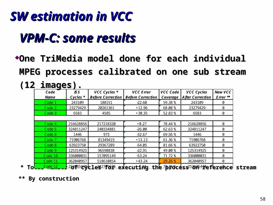
VPM-C: some resultsVPM-C: some results
One TriMedia model done for each individual MPEG One TriMedia model done for each individual MPEG
processes calibrated on one sub stream (12 images).processes calibrated on one sub stream (12 images).
* Total number of cycles for executing the process on reference stream* Total number of cycles for executing the process on reference stream
** By construction** By construction
Code ISS VCC Cycles * VCC Error VCC Code VCC Cycles New VCCName Cycles * Before Correction Before Correction Coverage After Correction Error **Code 1 243109 188151 -22.60 59.38 % 243109 0Code 2 23279429 20261361 +12.96 68.08 % 23279429 0Code 3 6583 4585 +30.35 52.83 % 6583 0
Code 4 216628856 217218320 +0.27 78.44 % 216628856 0Code 5 324811247 240334881 -26.00 62.63 % 324811247 0Code 6 1446 973 -32.67 69.56 % 1446 0Code 7 71906768 81349419 +13.13 61.36 % 71906768 0Code 8 63923750 29367289 -54.05 81.66 % 63923750 0Code 9 125314925 96598838 -22.91 49.00 % 125314925 0Code 10 336000031 157095149 -53.24 71.72 % 336000031 0Code 11 362040957 518610854 +43.24 29.26 % 362040957 0Code 12 253535440 242771676 -4.24 78.36 % 253535440 0
59
SW estimation in VCCSW estimation in VCC
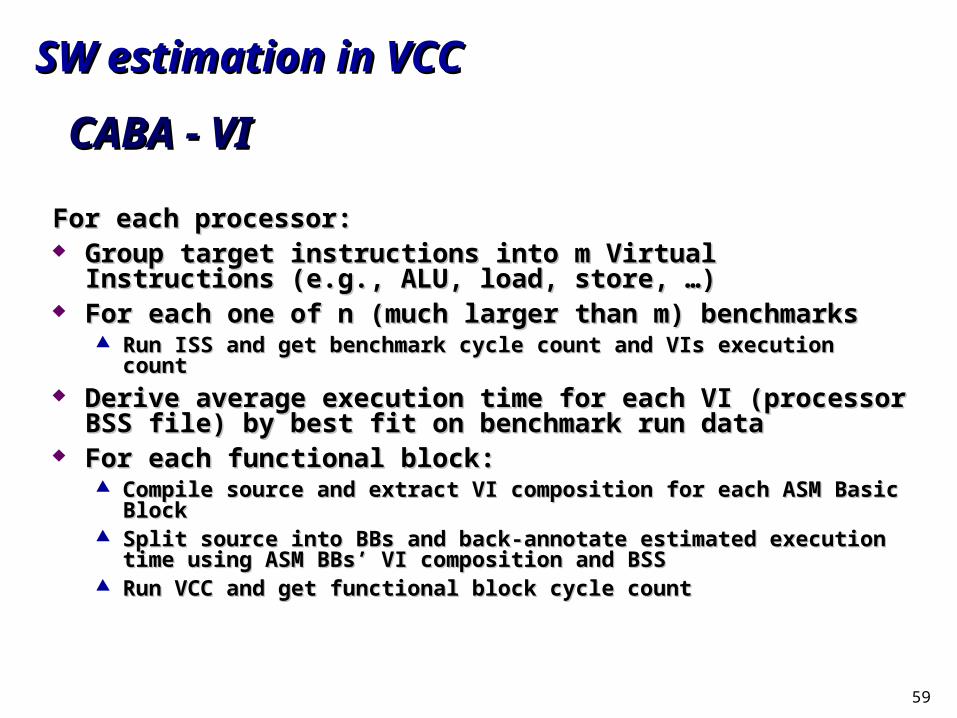
CABA - VICABA - VI
For each processor:For each processor: Group target instructions into m Virtual Instructions (e.g., ALU, load, Group target instructions into m Virtual Instructions (e.g., ALU, load,
store, …)store, …) For each one of n (much larger than m) benchmarksFor each one of n (much larger than m) benchmarks
Run ISS and get benchmark cycle count and VIs execution countRun ISS and get benchmark cycle count and VIs execution count Derive average execution time for each VI (processor BSS file) by best Derive average execution time for each VI (processor BSS file) by best
fit on benchmark run datafit on benchmark run data For each functional block:For each functional block:
Compile source and extract VI composition for each ASM Basic BlockCompile source and extract VI composition for each ASM Basic Block Split source into BBs and back-annotate estimated execution time using ASM BBs’ Split source into BBs and back-annotate estimated execution time using ASM BBs’
VI composition and BSSVI composition and BSS Run VCC and get functional block cycle countRun VCC and get functional block cycle count
60
SW estimation in VCCSW estimation in VCC
CABA - VICABA - VI
CABA-VI: uses a calibration-like procedure to obtain average CABA-VI: uses a calibration-like procedure to obtain average execution timing for each target instruction (or instruction class execution timing for each target instruction (or instruction class – Virtual Instruction (VI)). Unlike the similar VPM technique, the – Virtual Instruction (VI)). Unlike the similar VPM technique, the VI’s are target-dependent. The resulted BSS is used to VI’s are target-dependent. The resulted BSS is used to generate the performance annotations (delay, power, bus generate the performance annotations (delay, power, bus traffic) and its accuracy is not limited to the calibration codes.traffic) and its accuracy is not limited to the calibration codes.
In both cases, part of the CCISS infrastructure is re-used to:In both cases, part of the CCISS infrastructure is re-used to: parse the assembler,parse the assembler, identify the basic blocks, identify the basic blocks, identify and remove the cross-reference tags, identify and remove the cross-reference tags, handle embedded waits and other constructs, handle embedded waits and other constructs, generate code for bus traffic.generate code for bus traffic.
61
SW estimation in VCCSW estimation in VCC
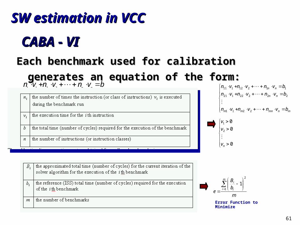
CABA - VICABA - VI
Each benchmark used for calibration generates an equation of the Each benchmark used for calibration generates an equation of the
form:form:bvnvnvn
nn
2211
mnmnmm
nn
nn
bvnvnvn
bvnvnvn
bvnvnvn
2211
22222121
11212111
0
0
0
2
1
nv
v
v
m
b
B
e
m
i i
i
1
2
1
Error Function to Minimize
62
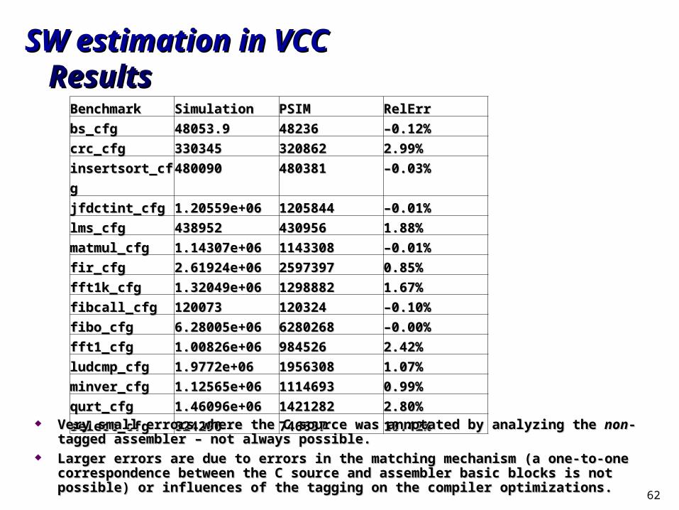
SW estimation in VCCSW estimation in VCCResultsResults
BenchmarkBenchmark SimulationSimulation PSIMPSIM RelErrRelErr
bs_cfgbs_cfg 48053.948053.9 4823648236 ––0.12% 0.12%
crc_cfgcrc_cfg 330345330345 320862320862 2.99% 2.99%
insertsort_cfginsertsort_cfg 480090480090 480381480381 ––0.03% 0.03%
jfdctint_cfgjfdctint_cfg 1.20559e+061.20559e+06 12058441205844 ––0.01%0.01%
lms_cfglms_cfg 438952438952 430956430956 1.88% 1.88%
matmul_cfgmatmul_cfg 1.14307e+061.14307e+06 11433081143308 ––0.01% 0.01%
fir_cfgfir_cfg 2.61924e+062.61924e+06 25973972597397 0.85%0.85%
fft1k_cfgfft1k_cfg 1.32049e+061.32049e+06 12988821298882 1.67%1.67%
fibcall_cfgfibcall_cfg 120073120073 120324120324 ––0.10%0.10%
fibo_cfgfibo_cfg 6.28005e+066.28005e+06 62802686280268 ––0.00%0.00%
fft1_cfgfft1_cfg 1.00826e+061.00826e+06 984526984526 2.42%2.42%
ludcmp_cfgludcmp_cfg 1.9772e+061.9772e+06 19563081956308 1.07%1.07%
minver_cfgminver_cfg 1.12565e+061.12565e+06 11146931114693 0.99% 0.99%
qurt_cfgqurt_cfg 1.46096e+061.46096e+06 14212821421282 2.80%2.80%
select_cfgselect_cfg 824290824290 746637746637 10.42%10.42% Very small errors where the C source was annotated by analyzing the Very small errors where the C source was annotated by analyzing the nonnon-tagged assembler – not -tagged assembler – not
always possible.always possible. Larger errors are due to errors in the matching mechanism (a one-to-one correspondence between Larger errors are due to errors in the matching mechanism (a one-to-one correspondence between
the C source and assembler basic blocks is not possible) or influences of the tagging on the compiler the C source and assembler basic blocks is not possible) or influences of the tagging on the compiler optimizations.optimizations.
63
SW estimation in VCCSW estimation in VCCConclusionsConclusions
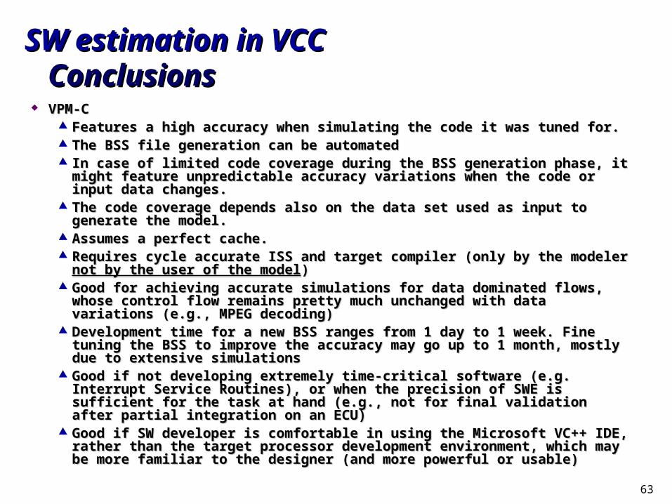
VPM-CVPM-C Features a high accuracy when simulating the code it was tuned for.Features a high accuracy when simulating the code it was tuned for. The BSS file generation can be automatedThe BSS file generation can be automated In case of limited code coverage during the BSS generation phase, it might feature In case of limited code coverage during the BSS generation phase, it might feature
unpredictable accuracy variations when the code or input data changes.unpredictable accuracy variations when the code or input data changes. The code coverage depends also on the data set used as input to generate the The code coverage depends also on the data set used as input to generate the
model.model. Assumes a perfect cache.Assumes a perfect cache. Requires cycle accurate ISS and target compiler (only by the modeler Requires cycle accurate ISS and target compiler (only by the modeler not by the not by the
user of the modeluser of the model)) Good for achieving accurate simulations for data dominated flows, whose control Good for achieving accurate simulations for data dominated flows, whose control
flow remains pretty much unchanged with data variations (e.g., MPEG decoding)flow remains pretty much unchanged with data variations (e.g., MPEG decoding) Development time for a new BSS ranges from 1 day to 1 week. Fine tuning the BSS Development time for a new BSS ranges from 1 day to 1 week. Fine tuning the BSS
to improve the accuracy may go up to 1 month, mostly due to extensive simulationsto improve the accuracy may go up to 1 month, mostly due to extensive simulations Good if not developing extremely time-critical software (e.g. Interrupt Service Good if not developing extremely time-critical software (e.g. Interrupt Service
Routines), or when the precision of SWE is sufficient for the task at hand (e.g., not Routines), or when the precision of SWE is sufficient for the task at hand (e.g., not for final validation after partial integration on an ECU)for final validation after partial integration on an ECU)
Good if SW developer is comfortable in using the Microsoft VC++ IDE, rather than Good if SW developer is comfortable in using the Microsoft VC++ IDE, rather than the target processor development environment, which may be more familiar to the the target processor development environment, which may be more familiar to the designer (and more powerful or usable)designer (and more powerful or usable)
64
SW estimation in VCCSW estimation in VCCConclusionsConclusions
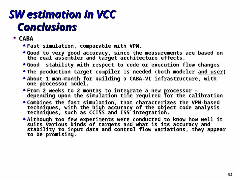
CABACABA Fast simulation, comparable with VPM.Fast simulation, comparable with VPM. Good to very good accuracy, since the measurements are based on the real Good to very good accuracy, since the measurements are based on the real
assembler and target architecture effects.assembler and target architecture effects. Good stability with respect to code or execution flow changes Good stability with respect to code or execution flow changes The production target compiler is needed (both modeler The production target compiler is needed (both modeler and userand user)) About 1 man-month for building a CABA-VI infrastructure, with one processor About 1 man-month for building a CABA-VI infrastructure, with one processor
model.model. From 2 weeks to 2 months to integrate a new processor – depending upon the From 2 weeks to 2 months to integrate a new processor – depending upon the
simulation time required for the calibrationsimulation time required for the calibration Combines the fast simulation, that characterizes the VPM-based techniques, with the Combines the fast simulation, that characterizes the VPM-based techniques, with the
high accuracy of the object code analysis techniques, such as CCISS and ISS high accuracy of the object code analysis techniques, such as CCISS and ISS integration.integration.
Although too few experiments were conducted to know how well it suits various Although too few experiments were conducted to know how well it suits various kinds of targets and what is its accuracy and stability to input data and control flow kinds of targets and what is its accuracy and stability to input data and control flow variations, they appear to be promising.variations, they appear to be promising.
65
OutlineOutline
SW estimation overviewSW estimation overview
Program path analysisProgram path analysis
Micro-architecture modelingMicro-architecture modeling
Implementation examples: CinderellaImplementation examples: Cinderella
SW estimation in VCCSW estimation in VCC
SW estimation in AISW estimation in AI
SW estimation in POLISSW estimation in POLIS
66
SW estimation in AISW estimation in AI
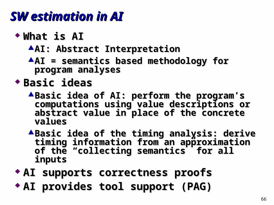
What is AIWhat is AIAI: Abstract InterpretationAI: Abstract InterpretationAI = semantics based methodology for program analysesAI = semantics based methodology for program analyses
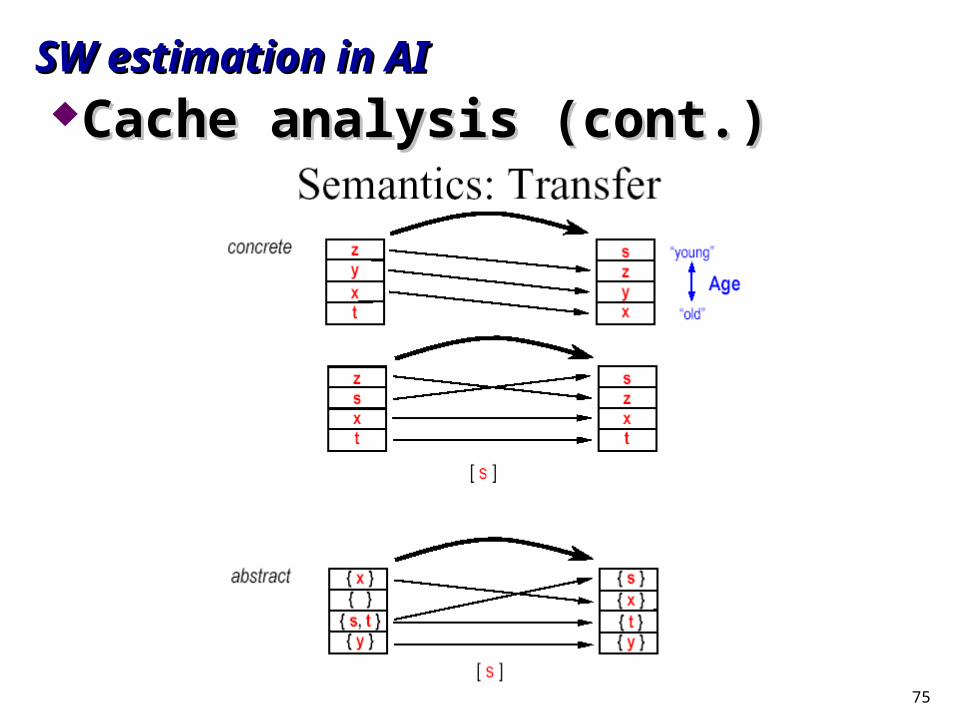
Basic ideasBasic ideasBasic idea of AI: perform the program’s computations using Basic idea of AI: perform the program’s computations using
value descriptions or abstract value in place of the concrete value descriptions or abstract value in place of the concrete valuesvalues
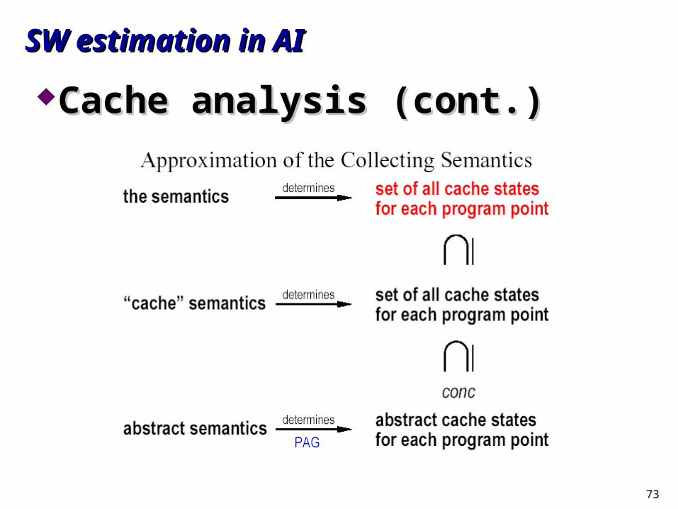
Basic idea of the timing analysis: derive timing information Basic idea of the timing analysis: derive timing information from an approximation of the “collecting semantics” for all from an approximation of the “collecting semantics” for all inputsinputs
AI supports correctness proofsAI supports correctness proofs AI provides tool support (PAG)AI provides tool support (PAG)
67
SW estimation in AISW estimation in AI
68
SW estimation in AISW estimation in AI
69
SW estimation in AISW estimation in AI
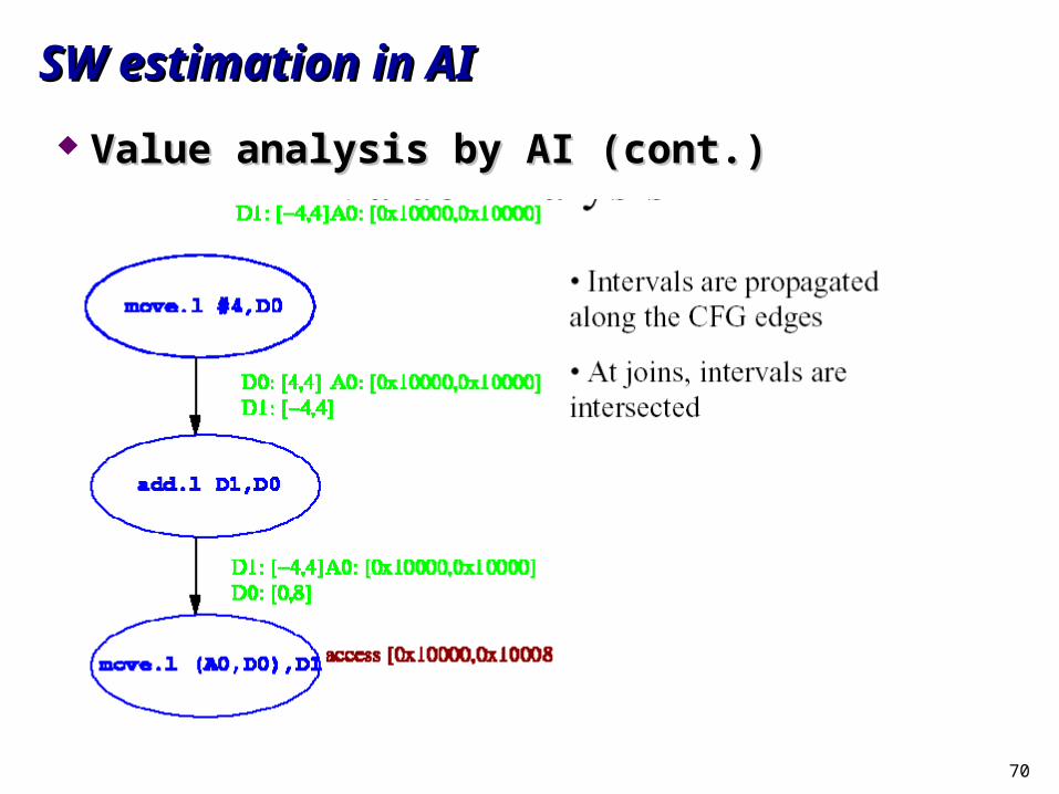
Value analysis by AIValue analysis by AIMotivationMotivation
Provide exact access information to cache/pipeline analysisProvide exact access information to cache/pipeline analysis Detection of infeasible pathDetection of infeasible path
GoalGoal calculate lower and upper bounds for the values occurring in the calculate lower and upper bounds for the values occurring in the
program (addresses, registers, local and global variables)program (addresses, registers, local and global variables)MethodMethod
AI interval analysis automatically generated with PAGAI interval analysis automatically generated with PAGIf partial programs are analyzed, value of stack pointer If partial programs are analyzed, value of stack pointer
should be suppliedshould be supplied
70
SW estimation in AISW estimation in AI
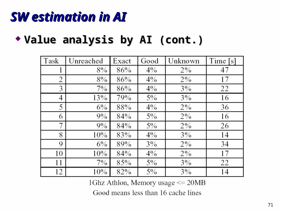
Value analysis by AI (cont.)Value analysis by AI (cont.)
71
SW estimation in AISW estimation in AI
Value analysis by AI (cont.)Value analysis by AI (cont.)
72
SW estimation in AISW estimation in AI
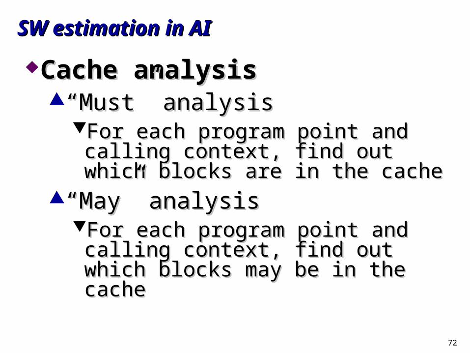
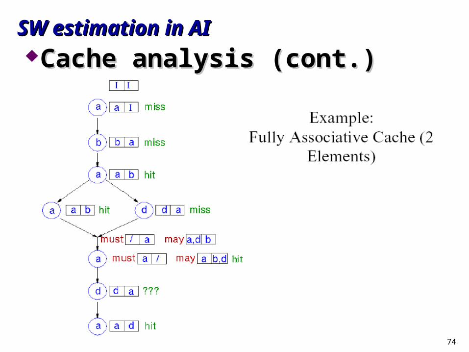
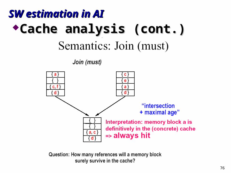
Cache analysisCache analysis““Must” analysisMust” analysis
For each program point and calling context, For each program point and calling context, find out which blocks are in the cachefind out which blocks are in the cache
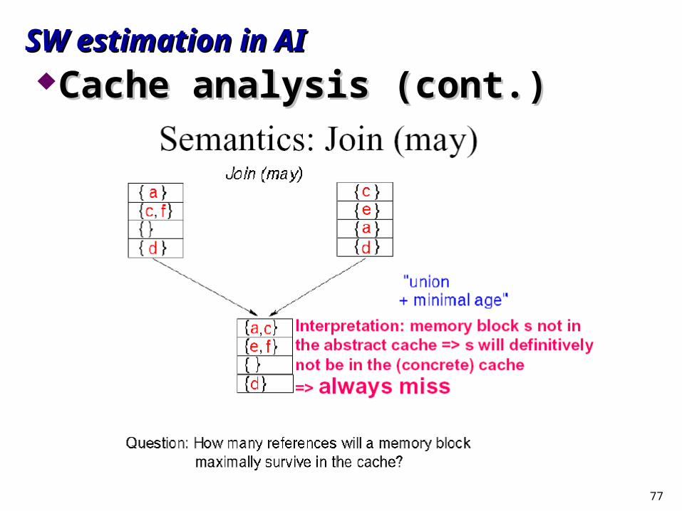
““May” analysisMay” analysisFor each program point and calling context, For each program point and calling context,
find out which blocks may be in the cachefind out which blocks may be in the cache
73
SW estimation in AISW estimation in AI
Cache analysis (cont.)Cache analysis (cont.)
74
SW estimation in AISW estimation in AICache analysis (cont.)Cache analysis (cont.)
75
SW estimation in AISW estimation in AICache analysis (cont.)Cache analysis (cont.)
76
SW estimation in AISW estimation in AICache analysis (cont.)Cache analysis (cont.)
77
SW estimation in AISW estimation in AICache analysis (cont.)Cache analysis (cont.)
78
ReferencesReferences
R. Ernst, W. Ye, R. Ernst, W. Ye, Embedded program timing analysis based on path Embedded program timing analysis based on path
clustering and architecture classificationclustering and architecture classification, ICCAD 1997, ICCAD 1997
S. Malik, M. Martonosi, and Y. T. S. Li, S. Malik, M. Martonosi, and Y. T. S. Li, Newblock Static timing Newblock Static timing
analysis of embedded softwareanalysis of embedded software, DAC 1997, DAC 1997
T. Ball and J. Larus, T. Ball and J. Larus, Efficient Path ProfilingEfficient Path Profiling, MICRO-29, 1996., MICRO-29, 1996.
P. Cousot, R. Cousot, P. Cousot, R. Cousot, Verification of Embedded Software: Problems Verification of Embedded Software: Problems
and Perspectives,and Perspectives, EMSOFT 2001 EMSOFT 2001
H. Theiling, C. Ferdinand, and R. Wilhelm, Fast and Precise WCET H. Theiling, C. Ferdinand, and R. Wilhelm, Fast and Precise WCET
Prediction by Separate Cache and Path Analyses, Real-Time Prediction by Separate Cache and Path Analyses, Real-Time
Systems, 18(2/3), May 2000.Systems, 18(2/3), May 2000.
79
OutlineOutline
SW estimation overviewSW estimation overview
Program path analysisProgram path analysis
Micro-architecture modelingMicro-architecture modeling
Implementation examples: CinderellaImplementation examples: Cinderella
SW estimation in VCCSW estimation in VCC
SW estimation in AISW estimation in AI
SW estimation in POLISSW estimation in POLIS

80
SW synthesis
CFSM
Sw code
S-graph synthesis and optimization
S-graph
Code generation
Timing / code size information
Estimation
SW estimation in POLISSW estimation in POLIS
S-graph Level EstimationS-graph Level Estimation
81
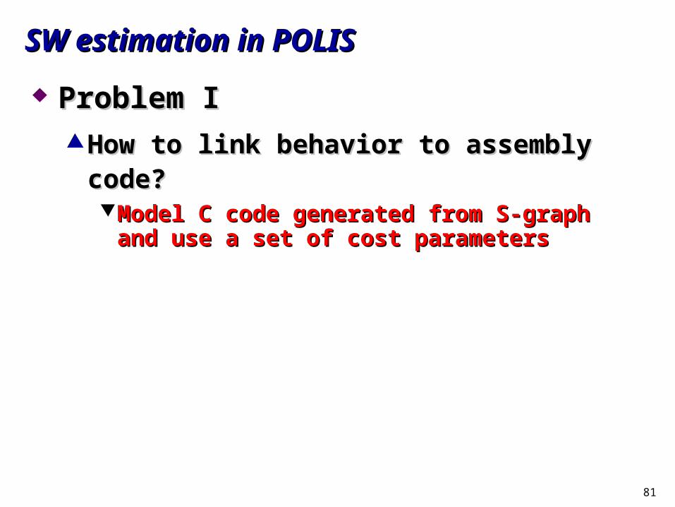
SW estimation in POLISSW estimation in POLIS
Problem IProblem I How to link behavior to assembly code?How to link behavior to assembly code?
Model C code generated from S-graph and use a set of Model C code generated from S-graph and use a set of cost parameterscost parameters
82
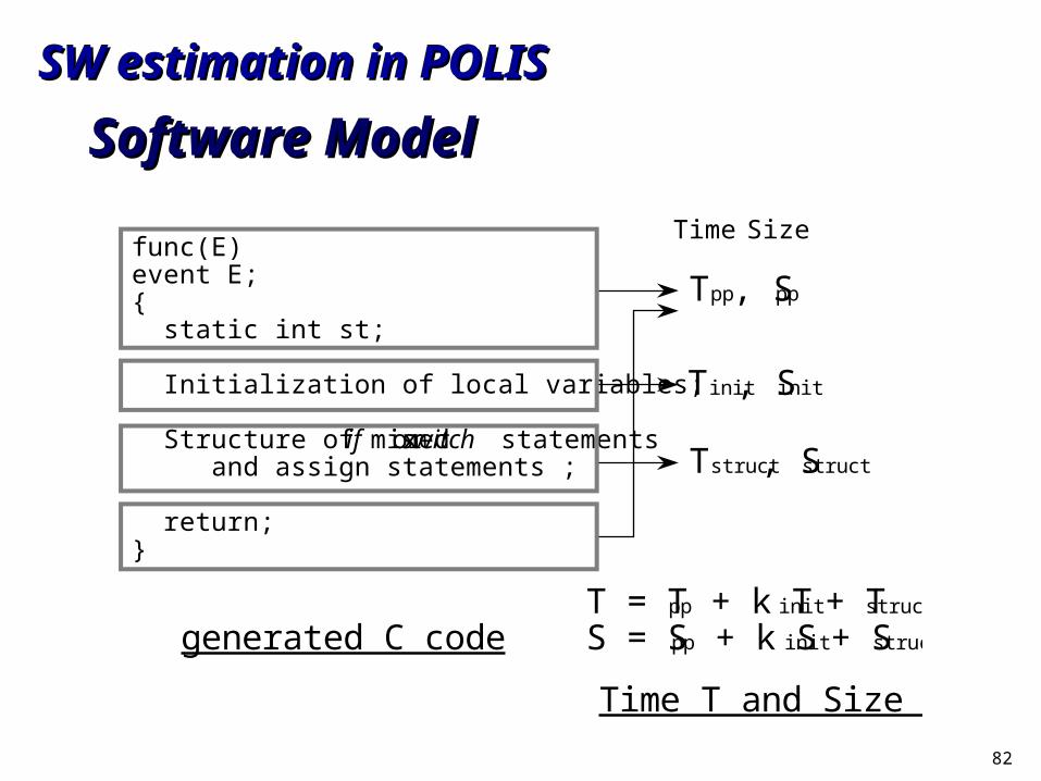
Software ModelSoftware Model
func(E) event E; { static int st; Initialization of local variables; Structure of mixed if or switch statements and assign statements ; return; }
generated C codeT = Tpp + k Tinit + Tstruct S = Spp + k Sinit + Sstruct
Time T and Size S
Tpp, Spp
Tinit, Sinit
Tstruct, Sstruct
Time Size
SW estimation in POLISSW estimation in POLIS
83
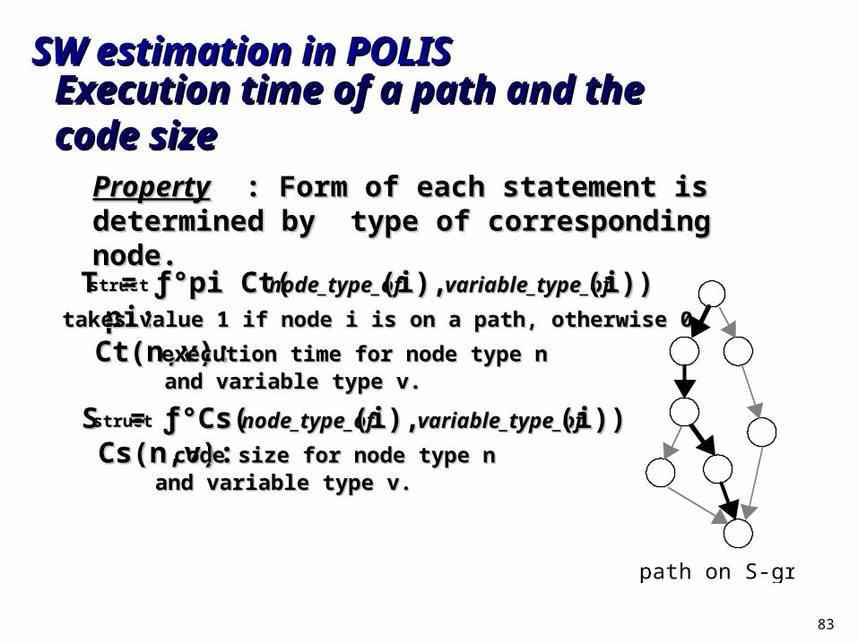
Execution time of a path and the code sizeExecution time of a path and the code size
PropertyProperty : Form of each statement is determined : Form of each statement is determined by type of corresponding node.by type of corresponding node.
TTstruct struct = ƒ°pi Ct(= ƒ°pi Ct( pi: pi: takes value 1 if node i is on a path, otherwise 0.takes value 1 if node i is on a path, otherwise 0. Ct(n,v): Ct(n,v): execution time for node type n execution time for node type n and variable type v.and variable type v.
SSstructstruct= ƒ°Cs(= ƒ°Cs(node_type_of node_type_of (i), (i), variable_type_of variable_type_of (i)) (i)) Cs(n,v): Cs(n,v): code size for node type n code size for node type n and variable type v.and variable type v.
path on S-graph
node_type_of node_type_of (i), (i), variable_type_of variable_type_of (i)) (i))
SW estimation in POLISSW estimation in POLIS
84
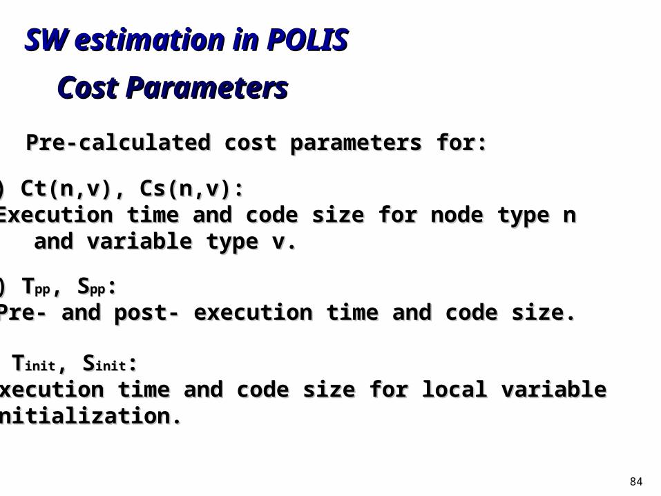
Cost ParametersCost Parameters
* Pre-calculated cost parameters for:* Pre-calculated cost parameters for:
(1) Ct(n,v), Cs(n,v): (1) Ct(n,v), Cs(n,v): Execution time and code size for node type n Execution time and code size for node type n and variable type v.and variable type v.
(2) T(2) Tpppp, S, Spppp: : Pre- and post- execution time and code size.Pre- and post- execution time and code size.
(3) T(3) Tinitinit, S, Sinitinit:: Execution time and code size for local variableExecution time and code size for local variable initialization.initialization.
SW estimation in POLISSW estimation in POLIS
85
SW estimation in POLISSW estimation in POLIS
Problem IIProblem II How to handle the variety of compilers and How to handle the variety of compilers and
CPUs?CPUs?prepare cost parameters for each target
86
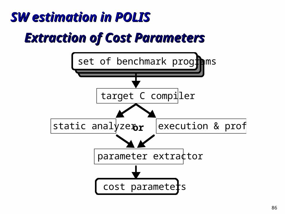
Extraction of Cost ParametersExtraction of Cost Parameters
set of benchmark programs
target C compiler
static analyzer execution & profilingor
parameter extractor
cost parameters
SW estimation in POLISSW estimation in POLIS
87
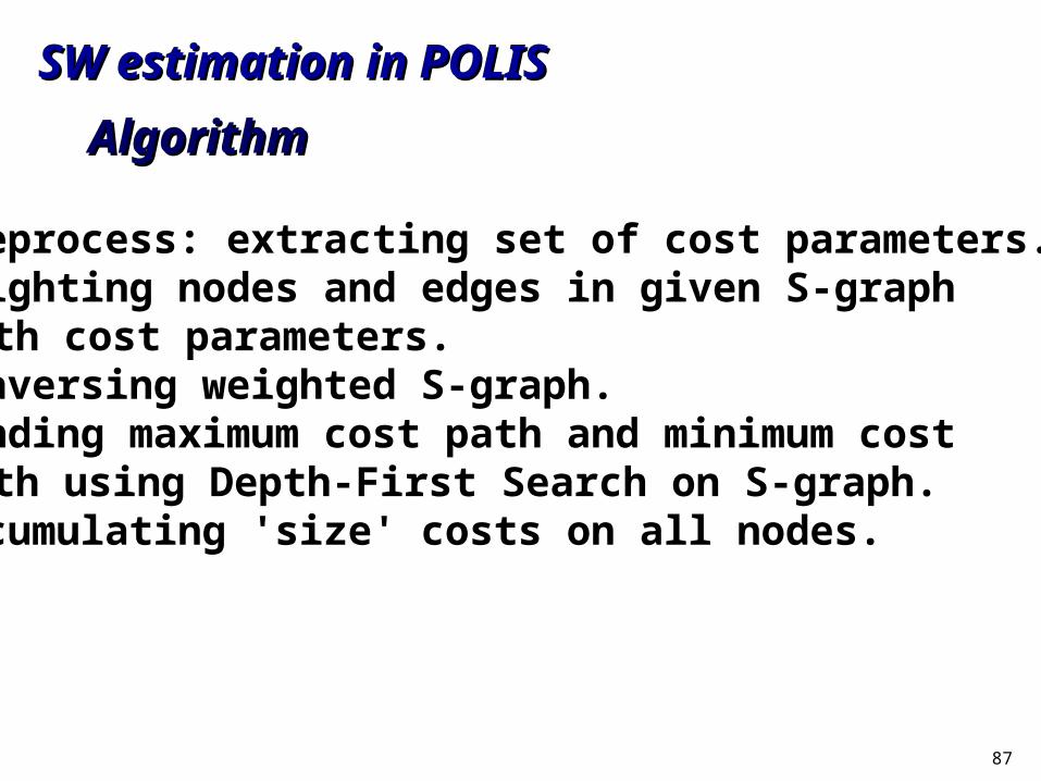
AlgorithmAlgorithm
Preprocess: extracting set of cost parameters. Weighting nodes and edges in given S-graph with cost parameters. Traversing weighted S-graph. Finding maximum cost path and minimum cost path using Depth-First Search on S-graph. Accumulating 'size' costs on all nodes.
SW estimation in POLISSW estimation in POLIS
88
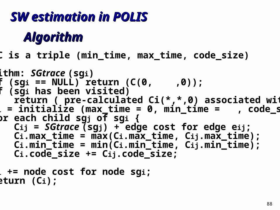
Cost C is a triple (min_time, max_time, code_size)
Algorithm: SGtrace (sgi) if (sgi == NULL) return (C(0, ,0)); if (sgi has been visited) return ( pre-calculated Ci(*,*,0) associated with sgi ); Ci = initialize (max_time = 0, min_time = , code_size = 0); for each child sgj of sgi { Cij = SGtrace (sgj) + edge cost for edge eij; Ci.max_time = max(Ci.max_time, Cij.max_time); Ci.min_time = min(Ci.min_time, Cij.min_time); Ci.code_size += Cij.code_size; } Ci += node cost for node sgi; return (Ci);
SW estimation in POLISSW estimation in POLIS
AlgorithmAlgorithm
89
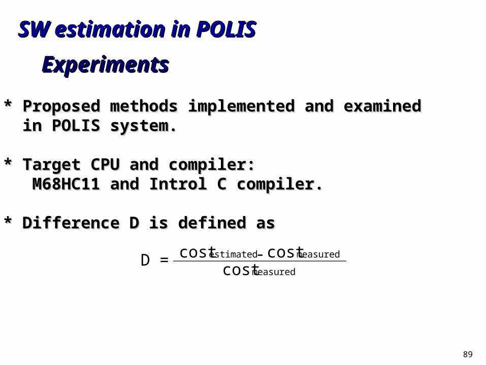
ExperimentsExperiments
* Proposed methods implemented and examined * Proposed methods implemented and examined in POLIS system.in POLIS system.
* Target CPU and compiler:* Target CPU and compiler: M68HC11 and Introl C compiler.M68HC11 and Introl C compiler.
* Difference D is defined as* Difference D is defined as
D = costestimated costmeasured-costmeasured
SW estimation in POLISSW estimation in POLIS
90
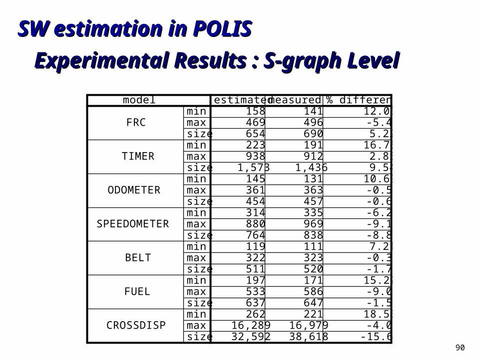
Experimental Results : S-graph LevelExperimental Results : S-graph Level
model estimated measured % differencemin 158 141 12.06
FRC max 469 496 -5.44size 654 690 5.22min 223 191 16.75
TIMER max 938 912 2.85size 1,573 1,436 9.54min 145 131 10.69
ODOMETER max 361 363 -0.55size 454 457 -0.66min 314 335 -6.27
SPEEDOMETER max 880 969 -9.18size 764 838 -8.83min 119 111 7.21
BELT max 322 323 -0.31size 511 520 -1.73min 197 171 15.20
FUEL max 533 586 -9.04size 637 647 -1.55min 262 221 18.55
CROSSDISP max 16,289 16,979 -4.06size 32,592 38,618 -15.60
SW estimation in POLISSW estimation in POLIS
91
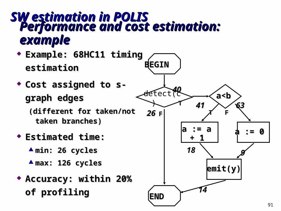
Performance and cost estimation: examplePerformance and cost estimation: example
4040
26264141 6363
14
18 9
Example: 68HC11 timing Example: 68HC11 timing
estimationestimation
Cost assigned to s-graph edgesCost assigned to s-graph edges
(different for taken/not taken (different for taken/not taken branches)branches)
Estimated time:Estimated time: min: 26 cyclesmin: 26 cycles
max: 126 cyclesmax: 126 cycles
Accuracy: within 20% of Accuracy: within 20% of
profilingprofiling
a := a a := a + 1+ 1
a := 0a := 0
detect(c)a<a<
bb
BEGINBEGIN
ENDEND
FF
TT
TT FF
emit(y)emit(y)
SW estimation in POLISSW estimation in POLIS
92
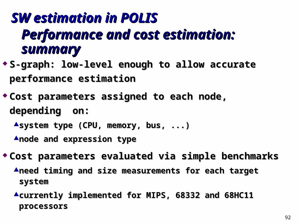
Performance and cost estimation: summaryPerformance and cost estimation: summary
S-graph: low-level enough to allow accurate performance S-graph: low-level enough to allow accurate performance
estimationestimation
Cost parameters assigned to each node, depending on:Cost parameters assigned to each node, depending on:system type (CPU, memory, bus, ...)system type (CPU, memory, bus, ...)
node and expression typenode and expression type
Cost parameters evaluated via simple benchmarksCost parameters evaluated via simple benchmarksneed timing and size measurements for each target systemneed timing and size measurements for each target system
currently implemented for MIPS, 68332 and 68HC11 processorscurrently implemented for MIPS, 68332 and 68HC11 processors
SW estimation in POLISSW estimation in POLIS


