Page 1
SOIL CLASSIFICATION BY USING ARTIFICIAL NEURAL NETWORKS
A THESIS SUBMITTED TO THE GRADUATE SCHOOL OF APPLIED SCIENCES
OF NEAR EAST UNIVERSITY
By ARİF ÖZYANKI
In Partial Fulfilment of the Requirements for the Degree of Master of Science
in Civil Engineering
NICOSIA, 2019
AR
İF Ö
ZY
AN
KI
SOIL
CL
ASSIFIC
AT
ION
BY
USIN
G
AR
TIFIC
IAL
NE
UR
AL
NE
TW
OR
KS
NE
U
2019
Page 2
SOIL CLASSIFICATION BY USING ARTIFICIAL NEURAL NETWORKS
A THESIS SUBMITTED TO THE GRADUATE SCHOOL OF APPLIED SCIENCES
OF NEAR EAST UNIVERSITY
By ARİF ÖZYANKI
In Partial Fulfilment of the Requirements for the Degree of Master of Science
in Civil Engineering
NICOSIA, 2019
Page 3
Arif ÖZYANKI: SOIL CLASSIFICATION BY USING ARTIFICIAL NEURAL NETWORKS
Approval of Director of Graduate School of Applied Sciences
Prof. Dr. Nadire ÇAVUŞ
We certify this thesis is satisfactory for the award of the degree of Masters of Science in Civil Engineering
Examining Committee in Charge:
Prof. Dr. Cavit ATALAR
Committee Chairman, Department of Civil Engineering, NEU
Assoc. Prof. Dr. Kamil DİMİLİLER
Department of Electrical and Electronic Engineering, NEU
Assist. Prof. Dr. Anoosheh IRAVANIAN Department of Civil Engineering, NEU
Page 4
I hereby declare that all information in this document has been obtained and presented in
accordance with academic rules and ethical conduct. I also declare that, as required by these
rules and conduct, I have fully cited and referenced all material and results that are not
original to this work.
Name, Last name: Arif Özyankı
Signature:
Date:
Page 5
ii
ACKNOWLEDGEMENTS
Foremost, I would like to express my sincere gratitude to my supervisor Prof. Dr. Cavit
Atalar for the continuous support of my master study and research, for his patience,
motivation, enthusiasm, and immense knowledge. His guidance helped me in all the time of
research and writing of this thesis. I could not have imagined having a better advisor and
mentor for my master study.
I would like to express my gratitude to Hilmi Dindar who is with me every time and to all
engineering faculty staff.
Last but not the least, I would like to thank my family: my parents Caner Özyankı and Nazif
Özyankı for giving birth to me at the first place and supporting me spiritually throughout my
life. I would also like to thank my dear sister Zerrin Karakaya, who is my source of
motivation with her children.
Page 7
iv
ABSTRACT
Soil properties are very important for the behavior of soils. Determination of the soil
properties depends firstly on the classification of the soils. Coarse and fine-grained soils are
fined out by sieve analysis. Fine-grained soils classification are done with their grain size
distribution which is obtained by hydrometer test as well as their Atterberg limits.
In this thesis, soil classification values have been reached at Atterberg limits values
estimated by using Artificial Neural Networks (ANN) training algorithm for fine-grained
soils of Turkish Republic of Northern Cyprus. For this study, 108 samples of clay, silt, and
sand percentages with liquid limit (LL) and plasticity index (PI) values were used. In the
beginning of the study, the LL and PI values were estimated from the grain size distribution
values. In the second part of the study soil classifications were found using estimated LL
and PI values. In order to obtain the optimum function in ANN model, it was aimed to give
high accuracy of the results by using different parameters and the highest correlation
coefficient (R2) values were examined. According to the results of the R2 values for LL were
0.85 for training, 0.86 for testing, and for PI were 0.80 for test and 0.82 for simulation. In
the second and final part of the study, the soil classifications were compared with the
estimated soil classifications found from the LL and PI. The results show that 75 out of 88
data used in the training (85.2%) and 18 out of 20 used in the test (90%) were correctly
estimated. ANN have been used in engineering areas frequently and reliably in recent years.
In particular, the ANN, which are characterized by learning characteristics, can be used
successfully in many prediction, estimation and classification processes, including cases
where good results cannot be achieved with classical regression methods.
Keywords: Soil classification; Atterberg limits; grain size distribution; fine grained soils;
Artificial Neural Networks; correlation coefficient
Page 8
v
ÖZET
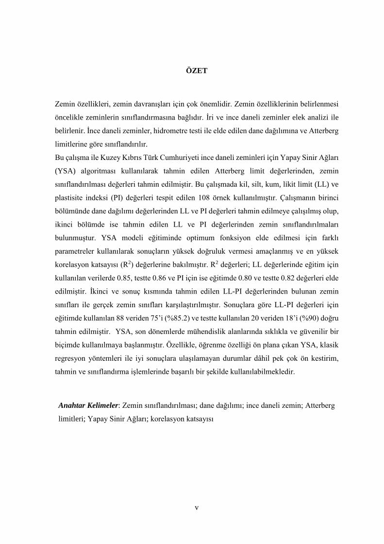
Zemin özellikleri, zemin davranışları için çok önemlidir. Zemin özelliklerinin belirlenmesi
öncelikle zeminlerin sınıflandırmasına bağlıdır. İri ve ince daneli zeminler elek analizi ile
belirlenir. İnce daneli zeminler, hidrometre testi ile elde edilen dane dağılımına ve Atterberg
limitlerine göre sınıflandırılır.
Bu çalışma ile Kuzey Kıbrıs Türk Cumhuriyeti ince daneli zeminleri için Yapay Sinir Ağları
(YSA) algoritması kullanılarak tahmin edilen Atterberg limit değerlerinden, zemin
sınıflandırılması değerleri tahmin edilmiştir. Bu çalışmada kil, silt, kum, likit limit (LL) ve
plastisite indeksi (PI) değerleri tespit edilen 108 örnek kullanılmıştır. Çalışmanın birinci
bölümünde dane dağılımı değerlerinden LL ve PI değerleri tahmin edilmeye çalışılmış olup,
ikinci bölümde ise tahmin edilen LL ve PI değerlerinden zemin sınıflandırılmaları
bulunmuştur. YSA modeli eğitiminde optimum fonksiyon elde edilmesi için farklı
parametreler kullanılarak sonuçların yüksek doğruluk vermesi amaçlanmış ve en yüksek
korelasyon katsayısı (R2) değerlerine bakılmıştır. R2 değerleri; LL değerlerinde eğitim için
kullanılan verilerde 0.85, testte 0.86 ve PI için ise eğitimde 0.80 ve testte 0.82 değerleri elde
edilmiştir. İkinci ve sonuç kısmında tahmin edilen LL-PI değerlerinden bulunan zemin
sınıfları ile gerçek zemin sınıfları karşılaştırılmıştır. Sonuçlara göre LL-PI değerleri için
eğitimde kullanılan 88 veriden 75’i (%85.2) ve testte kullanılan 20 veriden 18’i (%90) doğru
tahmin edilmiştir. YSA, son dönemlerde mühendislik alanlarında sıklıkla ve güvenilir bir
biçimde kullanılmaya başlanmıştır. Özellikle, öğrenme özelliği ön plana çıkan YSA, klasik
regresyon yöntemleri ile iyi sonuçlara ulaşılamayan durumlar dâhil pek çok ön kestirim,
tahmin ve sınıflandırma işlemlerinde başarılı bir şekilde kullanılabilmekledir.
Anahtar Kelimeler: Zemin sınıflandırılması; dane dağılımı; ince daneli zemin; Atterberg
limitleri; Yapay Sinir Ağları; korelasyon katsayısı
Page 9
vi
TABLE OF CONTENTS
ACKNOWLEDGEMENTS………………………………………………...... ii
ABSTRACT …………………………………………………………………... iv
ÖZET …………………………………………………………………………. v
TABLE OF CONTENTS ……………………………………………………. vi
LIST OF TABLES ……………………………………………………………. viii
LIST OF FIGURES …………………………………………………………... ix
LIST OF SYMBOLS AND ABBREVIATIONS ……………………………. xi
CHAPTER 1: INTRODUCTION
1.1. Background……………………………...……………………………........ 1
1.2. Problem Statement……………………………………………...…………. 3
1.3. Hypothesis ……………………………………………………...…………. 3
1.4. Research Objective ………………………………………………...……… 4
1.5. Organization of Study ………………………………………...…………… 4
CHAPTER 2: LITERATURE REVIEW
2.1. Soil Classification …………………………………………………………. 6
2.2. Atterberg Limit Tests …………………………………...…………………. 6
2.3. Artificial Neural Network in Geotechnical Engineering …...………..……. 7
2.4. Some Existing Correlations ……………………………………………….. 8
CHAPTER 3: MATERIALS AND METHODS
3.1. Area of Study ……………………………………………………………… 14
3.2. Testing Methods …………………………………………………………... 16
3.2.1. Grain size distribution ………………………………………………... 17
3.2.2. Atterberg limits ………………………………………………………. 18
3.3. Artificial Neural Network ………………………………………………… 19
3.3.1. Definition of ANN ………………………………………………….... 19
Page 10
vii
3.3.2. Main components of ANN ……………………………….…………... 20
3.3.3. Neural network types……………………………………………….. 24
CHAPTER 4: DATA ANALYSIS AND RESULTS
4.1. Data Analysis Methods …………………………………………………… 28
4.2. Multiple Linear Regression Analysis ……………………………………... 29
4.3. Artificial Neural Network Training Algorithm ……………………………. 32
4.3.1. Prediction to liquid limit and plasticity index ……………..………… 32
4.3.2. Determination of soil classification ………………………………….. 53
4.4. Results ……………………………………………………………………. 58
CHAPTER 5: CONCLUSIONS AND RECOMMENDATIONS
5.1. Conclusions …………...……………………………………………….. 59
5.2. Recommendations ...…………………………………………………… 60
REFERENCES ……………………………………………………………….. 61
APENDICES
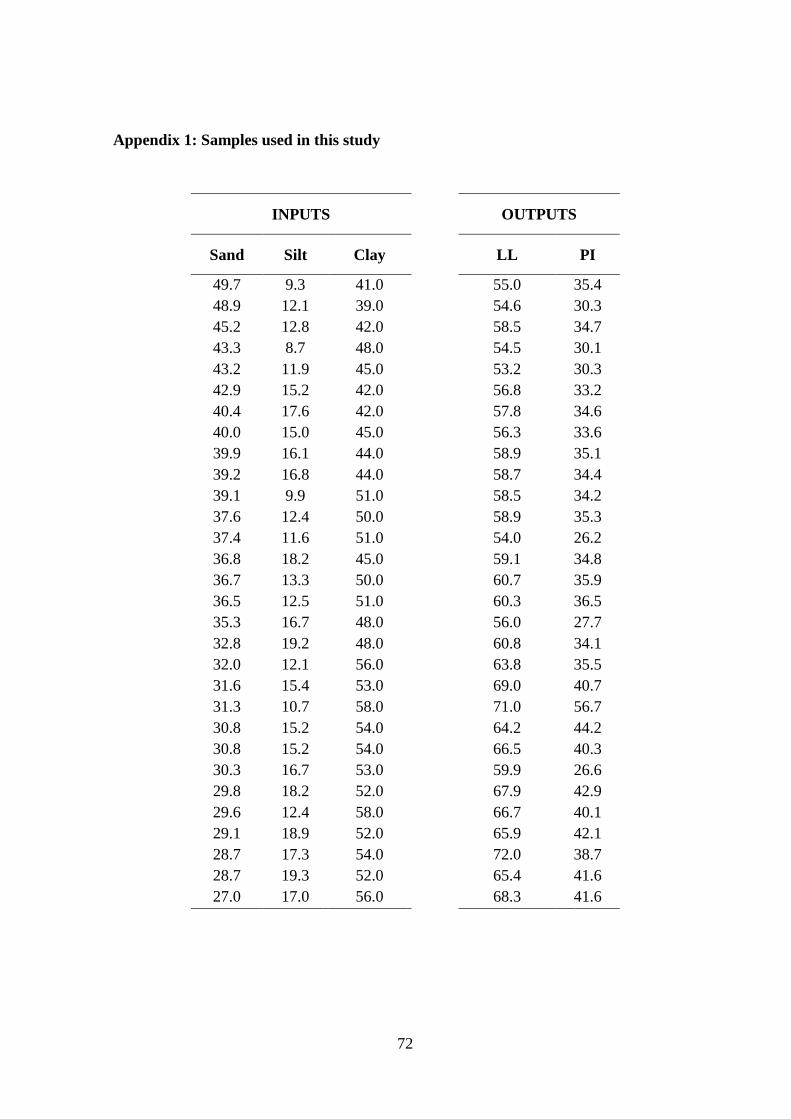
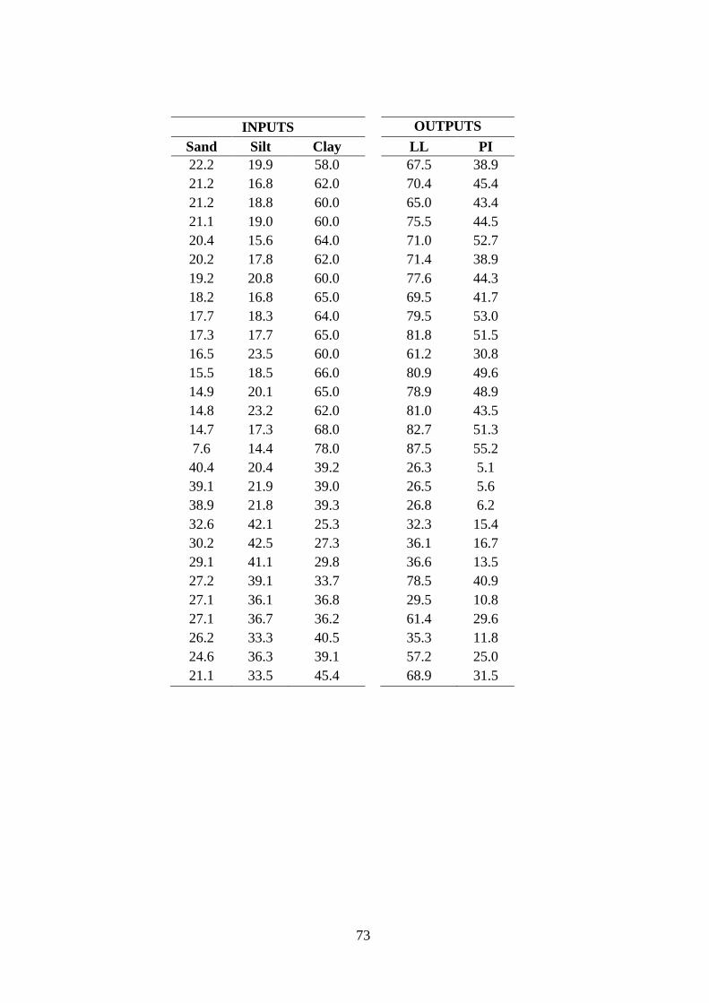
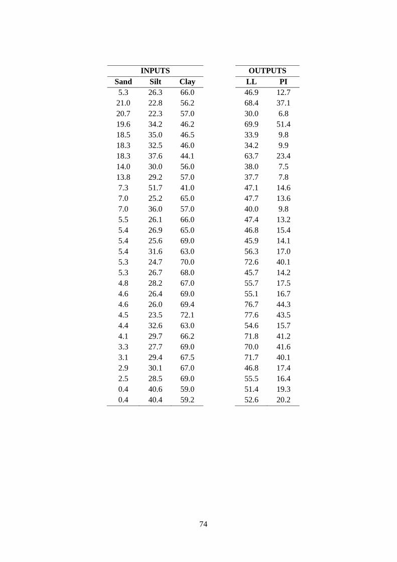
Appendix 1: Samples used in this study ….…………………………………….. 72
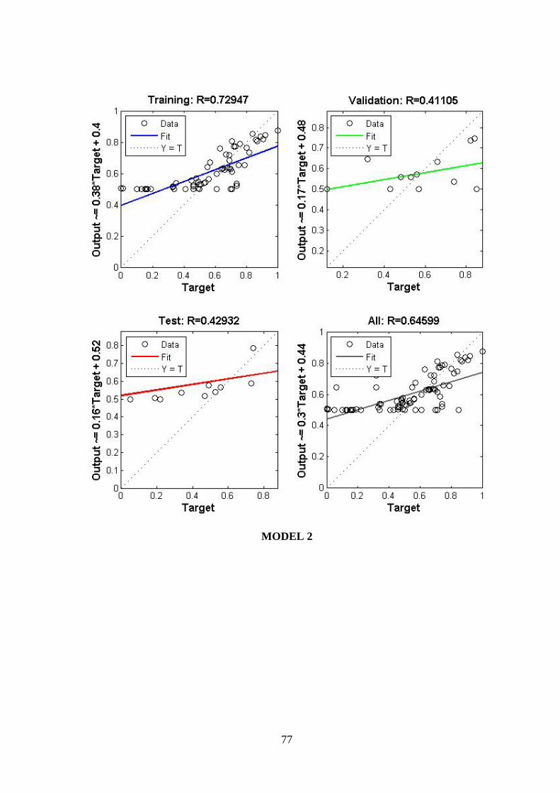
Appendix 2: Regression analysis results for LL ………………………………... 76
Appendix 3: Regression analysis results for PI ………………………………... 85
Page 11
viii
LIST OF TABLES
Table 2.1: The neural network models used in the determination of compaction
parameters …………………………………………………………
8
Table 3.1: Swelling potential of Cyprus clays ………………………………… 16
Table 3.2: Biological Nervous System with similar features of ANN ….……. 20
Table 4.1: Accuracy of coefficient determination ……………………………... 29
Table 4.2: Data properties ……………………………………………………... 30
Table 4.3: Multiple linear regression analysis results ………………………… 30
Table 4.4: Normalized input and output data for training …………………….. 34
Table 4.5: Normalized input and output data for test ………………………… 38
Table 4.6: ANN models for LL prediction ..…………………………………… 39
Table 4.7: ANN models for PI prediction ………………………………..……. 41
Table 4.8: ANN structure parameters …………………………………………. 43
Table 4.9: Comparison of the training data set for LL values ….………………. 46
Table 4.10: Comparison of the test data set LL values …………..…………….. 47
Table 4.11: Comparison of training data set PI values ……………...…………. 51
Table 4.12: Comparison of the test data set for PI values .………………..…… 52
Table 4.13: Comparison of soil classification with training data set …………... 56
Table 4.14: Comparison of soil classification with test data set ………………. 57
Page 12
ix
LIST OF FIGURES
Figure 1.1: Algorithm of the study ……………………………………………. 5
Figure 2.1: Simple linear regression analysis results ; a) LL versus OMC, b)
PL versus OMC, c) LL versus MD, d) PL versus MDD ...……….
9
Figure 2.2: Comparison between measured compaction values, and the
estimated compaction values by Model II …………..……………
10
Figure 2.3: Observed OMC vs Predicted OMC values during a) Training, b)
Testing, and c) Simulation …………………..……………………..
10
Figure 2.4: Observed OMC vs Predicted MDD values during a) Training, b)
Testing, and c) Simulation ……….………………………………...
11
Figure 2.5: a) Experimental LL versus predicted LL, b) Experimental MDD
versus predicted MDD, and c) Experimental OMC versus predicted
OMC ………………………………………………………………
12
Figure 2.6: a) Measured FC versus predicted FC, b) Measured LL versus
predicted LL, c) Measured PI versus predicted PI …..……………..
13
Figure 3.1: Cyprus geological map …………………………………..……..… 14
Figure 3.2: Cyprus clays map …………………………………………………. 16
Figure 3.3: Biological nerve cell structure …………………………………….. 19
Figure 3.4: Sigmoid activation function …………………….………………… 22
Figure 3.5: Hyperbolic tangent sigmoid function ……………………………… 23
Figure 3.6: Linear (purelin) function………………………………………….. 23
Figure 3.7: Adaptive resonance theory (ART) network structure ……………… 24
Figure 3.8: RBF network structure ……………………………………………. 26
Figure 4.1: Multiple linear regression analysis results for LL ……………….. 31
Figure 4.2: Multiple linear regression analysis results for PI …………………. 31
Figure 4.3: Generalized base the study ………………………………………... 32
Figure 4.4: The generalized the ANN model ………………………………….. 33
Figure 4.5: Comparison ANN models for predict LL …………………………. 39
Figure 4.6: Regression analysis results; a) Model 5, and b) Model 3 .…………. 40
Figure 4.7: Comparison ANN models for predict ……………………………. 41
Figure 4.8: Regression analysis results; a) Model 2, and b) Model 7 ….……..... 42
Page 13
x
Figure 4.9: ANN model sample ……………………………………………….. 43
Figure 4.10: Data entry into the network ……………………………………… 44
Figure 4.11: Regression analysis result for LL …………….. ………………… 45
Figure 4.12: Comparison between real and predict data for LL ….……………. 48
Figure 4.13: Data entry into the network………………………………………. 49
Figure 4.14: Regression analysis result for PI …………………………………. 50
Figure 4.15: Comparison between real and predict data for PI …..…………….. 53
Figure 4.16: Unified Soil Classification System Symbol Chart ……………….. 53
Figure 4.17: Real data set classification which used for training ……………… 54
Figure 4.18: Real data set classification which used for testing ………………. 54
Figure 4.19: Predicted data set classification which used for training …………. 55
Figure 4.20: Predicted data set classification which used for testing …………. 55
Page 14
xi
LIST OF SYMBOLS AND ABBREVIATIONS
ANN: Artificial Neural Networks
ART: Adaptive Resonance Theory
CEC: Cation Exchange
CPT: Cone Penetration Test
D: Grain Size
Dr: Relative Density
FC: Fines Content
G: Specific Gravity
He: Effective Depth
LL: Liquid Limit
M: Temperature
MDD: Maximum Dry Density
Ms: Dry Soil Mass
N: Percentages of Grain Size Smaller Than D
OM: Organic Matter
OMC: Optimum Moist Content
PI: Plasticity Index
PL: Plastic Limit
R: Hydrometer Reading Correction
R2: Coefficient of Determination
RBF: Radial Basis Function
RNN: Recurrent Neural Network
SL: Shrinkage Limit
SPT: Standard Penetration Test
SSE: Sum of Squares of Model Errors
SST: Square Sum of The Errors
t: Sedimentation Time
USCS: The Unified Soil Classification System
Vk: Net Input
Page 15
xii
w: Weights
xi: ANNs Input Values
σ': Effective Stress
𝜂𝜂: Water Viscosity
ρw: Water Density
Page 16
1
CHAPTER 1
INTRODUCTION
1.1. Background
The soil is composed of gravel, sand, silt, and clay as a result of disintegration or by
disintegration, transportation, and deposition of rocks. There are several methods to find the
properties of soils. The methods followed in the examination of soils are complementary to
each other, it is impossible to obtain information about the behavior of soils without
determining the properties and changes of soil characteristics. Geotechnical engineers are
able to determine which characteristics have the most impact on soil behavior. The soils are
heterogeneous. It can be expected to vary within meters. Soils remain under various
influences such as loading, dewatering, drying, and freezing over the years. The reactions of
the soil in these cases are important both in the use of the soil as a building material and in
the structures to be built upon.
Soils can have infinitely different properties due to the composition of its mineral or organic
contents. It is difficult to apply probability methods to such a subject. It is also considered
that to determine the soil characteristics require long-term and expensive experiments.
Therefore, various researchers presented statistical methods in the form of regression
analysis in order to determine the soil properties which provide reliable results and also can
be obtained rapidly and inexpensively.
The buildings that make up the living areas of people are mostly built on soils. Accurate
estimation of the properties of the soils on which these buildings will be build will provide
economic gain for the design of the buildings and will guarantee their lives and assets for
the people living in it.
The soil classification system has been one of the communication languages among the
engineers in geotechnical engineering applications. The determination of soil classification
is not eliminating the need for detailed soil investigations and other laboratory tests on soil
samples which we determine the engineering properties. However, an engineer can
Page 17
2
determine the behavior of the soil in the case of structural loads in the application phase by
classified soil. It is an inevitable fact that clays, which are frequently encountered in soil
mechanics problems, have a wide range in terms of their engineering characteristics.
The grains forming the soil have a very different geometry and are of a wide variety of sizes.
Knowing the grain size distribution in the soil plays an important role in determining the
index properties of soils. The grain size distribution is the ratio of the weight of the grains
of various diameters to the total dry weight of the soil in percent. Soils are divided into two
types: coarse-grained soils (gravel and sand) and fine-grained soils (clay and silt). In order
to determine the grain size distribution of the coarse-grained soils according to the in
diameters, the sieve analysis is carried out and the hydrometer test is performed to determine
the grain size distribution of the fine-grained soils according to the diameters.
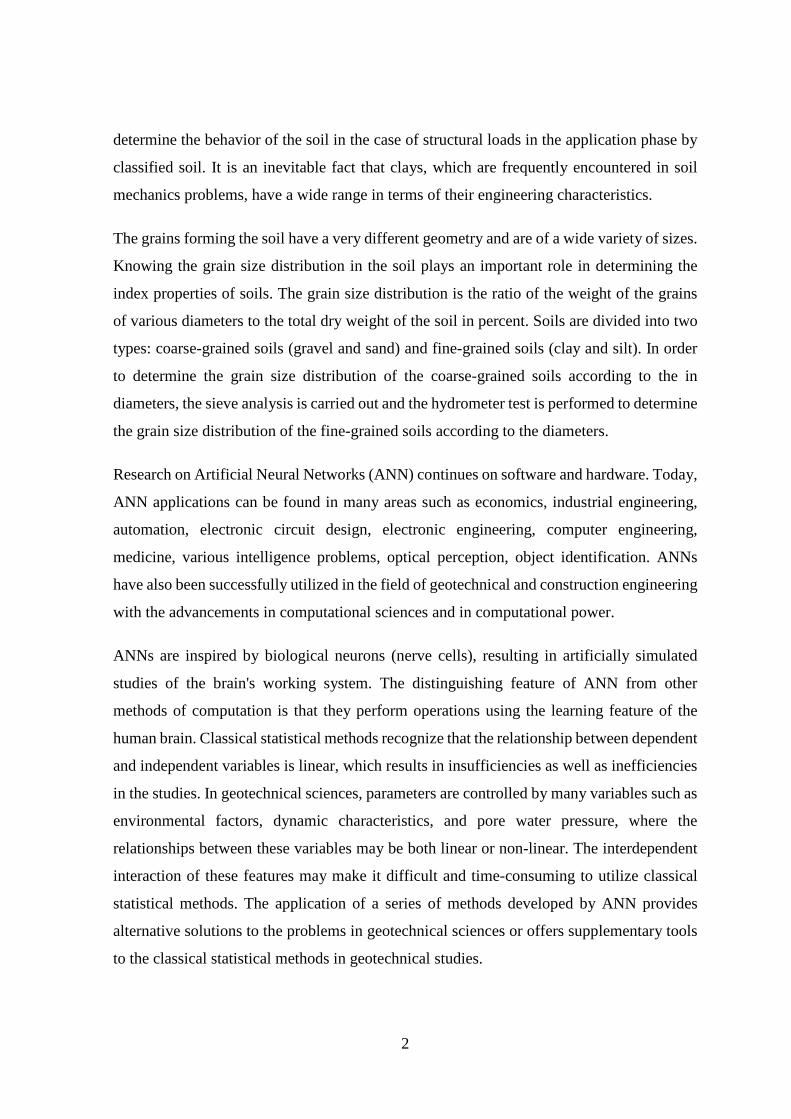
Research on Artificial Neural Networks (ANN) continues on software and hardware. Today,
ANN applications can be found in many areas such as economics, industrial engineering,
automation, electronic circuit design, electronic engineering, computer engineering,
medicine, various intelligence problems, optical perception, object identification. ANNs
have also been successfully utilized in the field of geotechnical and construction engineering
with the advancements in computational sciences and in computational power.
ANNs are inspired by biological neurons (nerve cells), resulting in artificially simulated
studies of the brain's working system. The distinguishing feature of ANN from other
methods of computation is that they perform operations using the learning feature of the
human brain. Classical statistical methods recognize that the relationship between dependent
and independent variables is linear, which results in insufficiencies as well as inefficiencies
in the studies. In geotechnical sciences, parameters are controlled by many variables such as
environmental factors, dynamic characteristics, and pore water pressure, where the
relationships between these variables may be both linear or non-linear. The interdependent
interaction of these features may make it difficult and time-consuming to utilize classical
statistical methods. The application of a series of methods developed by ANN provides
alternative solutions to the problems in geotechnical sciences or offers supplementary tools
to the classical statistical methods in geotechnical studies.
Page 18
3
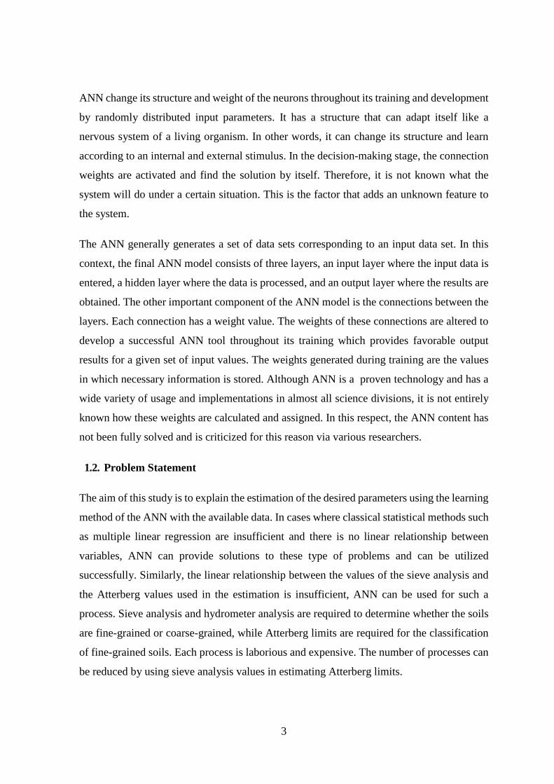
ANN change its structure and weight of the neurons throughout its training and development
by randomly distributed input parameters. It has a structure that can adapt itself like a
nervous system of a living organism. In other words, it can change its structure and learn
according to an internal and external stimulus. In the decision-making stage, the connection
weights are activated and find the solution by itself. Therefore, it is not known what the
system will do under a certain situation. This is the factor that adds an unknown feature to
the system.
The ANN generally generates a set of data sets corresponding to an input data set. In this
context, the final ANN model consists of three layers, an input layer where the input data is
entered, a hidden layer where the data is processed, and an output layer where the results are
obtained. The other important component of the ANN model is the connections between the
layers. Each connection has a weight value. The weights of these connections are altered to
develop a successful ANN tool throughout its training which provides favorable output
results for a given set of input values. The weights generated during training are the values
in which necessary information is stored. Although ANN is a proven technology and has a
wide variety of usage and implementations in almost all science divisions, it is not entirely
known how these weights are calculated and assigned. In this respect, the ANN content has
not been fully solved and is criticized for this reason via various researchers.
1.2. Problem Statement
The aim of this study is to explain the estimation of the desired parameters using the learning
method of the ANN with the available data. In cases where classical statistical methods such
as multiple linear regression are insufficient and there is no linear relationship between
variables, ANN can provide solutions to these type of problems and can be utilized
successfully. Similarly, the linear relationship between the values of the sieve analysis and
the Atterberg values used in the estimation is insufficient, ANN can be used for such a
process. Sieve analysis and hydrometer analysis are required to determine whether the soils
are fine-grained or coarse-grained, while Atterberg limits are required for the classification
of fine-grained soils. Each process is laborious and expensive. The number of processes can
be reduced by using sieve analysis values in estimating Atterberg limits.
Page 19
4
1.3. Hypothesis
In this thesis, Atterberg limits which are difficult to be predicted by classical statistical
methods will be calculated by using ANN and soil classification will be made from these
values.
1.4. Research Objectives
The main objective of this thesis is to estimate the Atterberg limits from the grain size
distribution values by the ANN method and to determine the soil classification from these
estimated values.
To achieve this goal;
i. Training the model of ANN with sieve analysis and Atterberg limits obtained from
previous projects in North Cyprus soils.
ii. Simulate the trained model with another set of data with the same characteristics.
iii. Determination of soil classification with estimated Atterberg limit values.
iv. The comparison of the determined soil classifications with the original soil
classification.
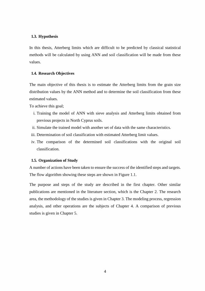
1.5. Organization of Study
A number of actions have been taken to ensure the success of the identified steps and targets.
The flow algorithm showing these steps are shown in Figure 1.1.
The purpose and steps of the study are described in the first chapter. Other similar
publications are mentioned in the literature section, which is the Chapter 2. The research
area, the methodology of the studies is given in Chapter 3. The modeling process, regression
analysis, and other operations are the subjects of Chapter 4. A comparison of previous
studies is given in Chapter 5.
Page 20
5
Figure 1.1: Algorithm of the study
Page 21
6
CHAPTER 2
LITERATURE REVIEW
2.1. Soil Classification
Soils with a grain size of less than 0.075 mm are defined as fine-grained soils (ASTM D422-
63; Holtz et al., 2011). Furthermore, in order to classify a soil sample as a fine-grained soil,
more than 50% of its dry weight should be finer than 0.075 mm. Fine-grained soils are a
mixture of clay and silt grains. The definition of the size limit between the clay and silt
particles is called the clay fraction and this difference is determined to be 0.005 (ASTM
D422-63) mm or 0.002 mm (Taylor, 1948). However, the cutoff between clay and silt
particles is very narrow. The plasticity properties of silt and clay are a better separator than
the particle size (Holtz et al., 2011).
2.2. Atterberg Limit Tests
Albert Atterberg (1911) originally defined six ‘Limits of consistency’ to classify fine-
grained soils, but in present engineering applications, only three of the limits, i.e. liquid (LL),
plastic (PL) and shrinkage (SL) limits are used. In fact, he was able to define several limits
of consistency and he has developed simple laboratory tests to define these limits. PL is the
transition limit for soils from semi-solid to plastic, and LL is the transition from the plastic
state to the liquid state (Casagrande, 1958; Archer, 1975; PCA, 1992; Campbell, 2001;
McBride, 2008; Das, 2010). These soil limits (soil consistency) are the water content rates
required for mechanical changes in the soil. The plastic range measured as the plastic limit
is the soil behavior limit where soil can return to plastic behavior without fracturing under
loading. These limits are used to classify fine-grained soils. Atterberg limits can also be used
to understand many soil mechanics and soil physical properties. Some of these features are
swelling and shrinkage potentials, shear strength, and compressibility (Archer, 1975; Wroth
and Wood, 1978; Campbell, 2001; McBride, 2008; Seybold, et al., 2008). These limits are
also indispensable for soil and substructure surveys. While investigating the fundamental
properties of soils, many researchers have used these limits. De la Rosa (1979), a research
conducted in Florida, said cation exchange capacity (CEC), organic matter (OM) and clay
content to cause considerable effects on PI. Studies on the soils in Canada and Nigeria have
Page 22
7
reported a significant relationship with the clay rate, LL, PL and PI values (Jong, et al.,
1990; Mbagwu and Abeh, 1998). In another study, Odell et al. (1960) concluded that the
clay content, the montmorillonite ratio in the soil and the OM ratio had a weighty effect on
LL and PI. In the study conducted with data on the database on the US, Seybold (2008) noted
that the clay content and CEC had a significant impact on LL and PI. Keller and Dexter
(2012) stated that there was a correlation between the clay content and LL, PL, and PI values.
2.3. Artificial Neural Network in Geotechnical Engineering
In the studies of civil engineering and geotechnical engineering, ANN has been widely used
since early 1990 (Lee and Lee, 1996; Najjar et al., 1996; Yuanyou et al., 1997; Yang and
Zhang, 1998; Hurtado et al., 2001; Rafiq et al., 2001; Lee et al., 2003; Basma and Kallas,
2004). In the previous studies, it is observed that ANN is frequently used in estimating the
compaction and uplift of pile foundations and axial and lateral load capacities (Goh, 1994,
1996; Chan et al., 1995; Goh et al., 1995; Lee and Lee, 1996; Teh et al., 1997; Abu-Kiefa,
1998; Nawari et al., 1999; Rahman et al., 2001; Hanna et al., 2004; Das and Basudhar, 2006;
Ahmad et al., 2007; Shahin and Jaksa, 2009), drilled pole (Goh et al., 2005; Shahin and
Jaksa, 2009), foundation settlements (Sivakugan et al., 1998) and anchors embedment
(Rahman et al., 2001; Shahin et al., 2004, 2005; Shahin and Jaksa, 2006).
Goh et al. (1995) studied the relative density (Dr) and average effective stress (σ') as input in
the ANN model performed on normally loaded and over-consolidated sands. They estimated
the Cone Penetration Test (CPT) and cone resistance (qc) as output. In this study, they used
93 data for training and 74 data for the testing. In this nonlinear relationship, the correlation
coefficient was obtained as 0.97 for training and 0.91 for the test.
The prediction of settlements in the foundations is affected by uncertainties, similar to other
complex issues of geotechnics. For this purpose, settlements prediction was tested with ANN
by some researchers. Sivakugan et al. (1998) predicted the settlement of the shallow
foundations on coarse-grained soils with ANN. In the development of the ANN tool, 79 data
sets were used where 69 of them were used for training and 10 datasets for testing. Five
parameters were used as input values that are applied net pressure, average standard
penetration test (SPT) values, foundation width, foundation form and foundation depth.
Page 23
8
The ANN method is applied to other applications in earth sciences; retaining walls (Ozturk,
2014; Ghaleini et al., 2018), dams (Ranković et al., 2014; Stojanovic et al., 2016), earthquake
(Dindar et al., 2017), geographical information systems (Aslantaş and Kurban, 2007),
mining (Rankine and Sivakugan, 2005; Afram et al., 2017), geoenvironmental engineering
(Shang et al., 2004), petroleum engineering (Kulga et al., 2018) and rock mechanics
(Kanungo et al., 2014).
Traditional statistical methods may be insufficient due to interactions between variables.
Prediction of physical properties of soil such as mineralogy, porosity, water content, grain
size etc. with statistical methods is difficult (Yingjie and Rosenbaum, 2002). ANN
algorithms can be used to estimate/determine various soil characteristics, including soil
classification (Cal, 1995).
2.4. Some Existing Correlations
In previous studies, the researchers used the ANN method in the estimation of soil properties
and soil classification. Different estimation methods were compared in previous studies with
ANN and classical regression analysis methods.
Cal (1995) had classified soil by using LL, PI and clay content. As a result of the study, he
classified the clay soils as; heavy clay (I), light clay (II), heavy sub-clay (III), medium sub-
clay (IV), light sub-clay (V), and sub-sandy clay (VI).
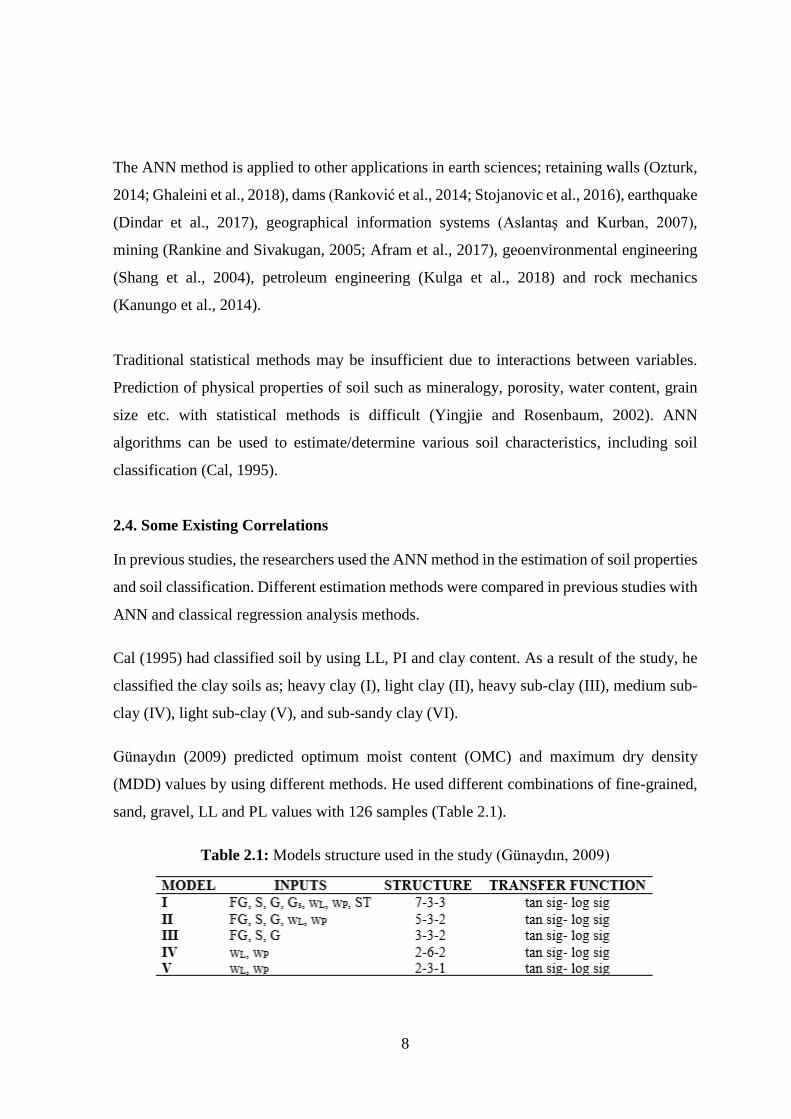
Günaydın (2009) predicted optimum moist content (OMC) and maximum dry density
(MDD) values by using different methods. He used different combinations of fine-grained,
sand, gravel, LL and PL values with 126 samples (Table 2.1).
Table 2.1: Models structure used in the study (Günaydın, 2009)
Page 24
9
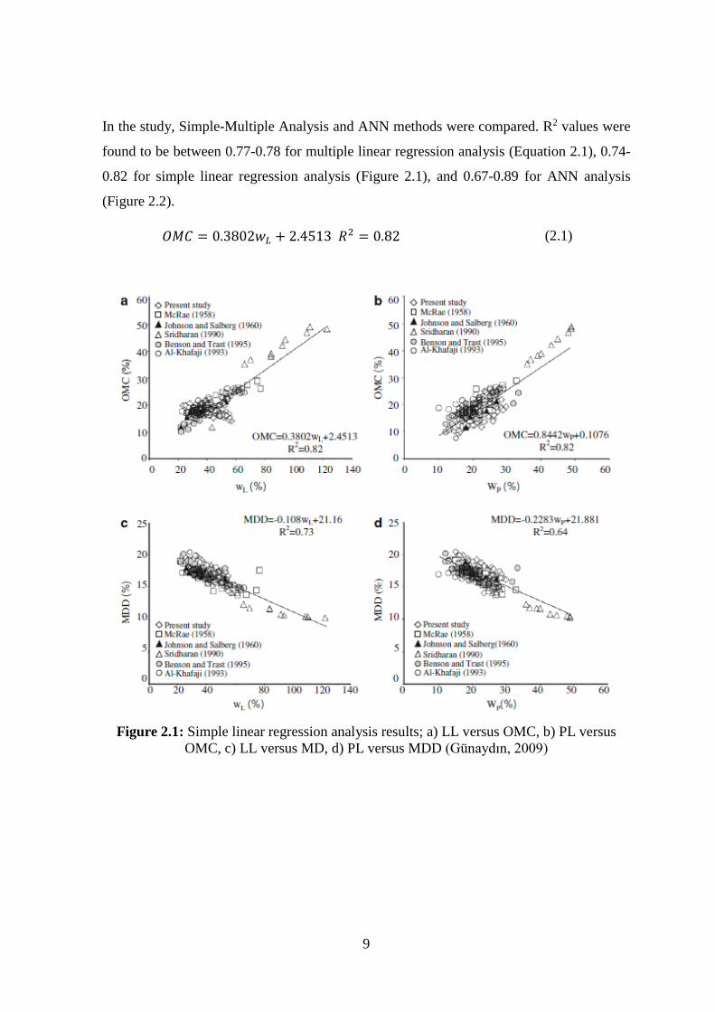
In the study, Simple-Multiple Analysis and ANN methods were compared. R2 values were
found to be between 0.77-0.78 for multiple linear regression analysis (Equation 2.1), 0.74-
0.82 for simple linear regression analysis (Figure 2.1), and 0.67-0.89 for ANN analysis
(Figure 2.2).
𝑂𝑂𝑂𝑂𝑂𝑂 = 0.3802𝑤𝑤𝐿𝐿 + 2.4513 𝑅𝑅2 = 0.82 (2.1)
Figure 2.1: Simple linear regression analysis results; a) LL versus OMC, b) PL versus
OMC, c) LL versus MD, d) PL versus MDD (Günaydın, 2009)
Page 25
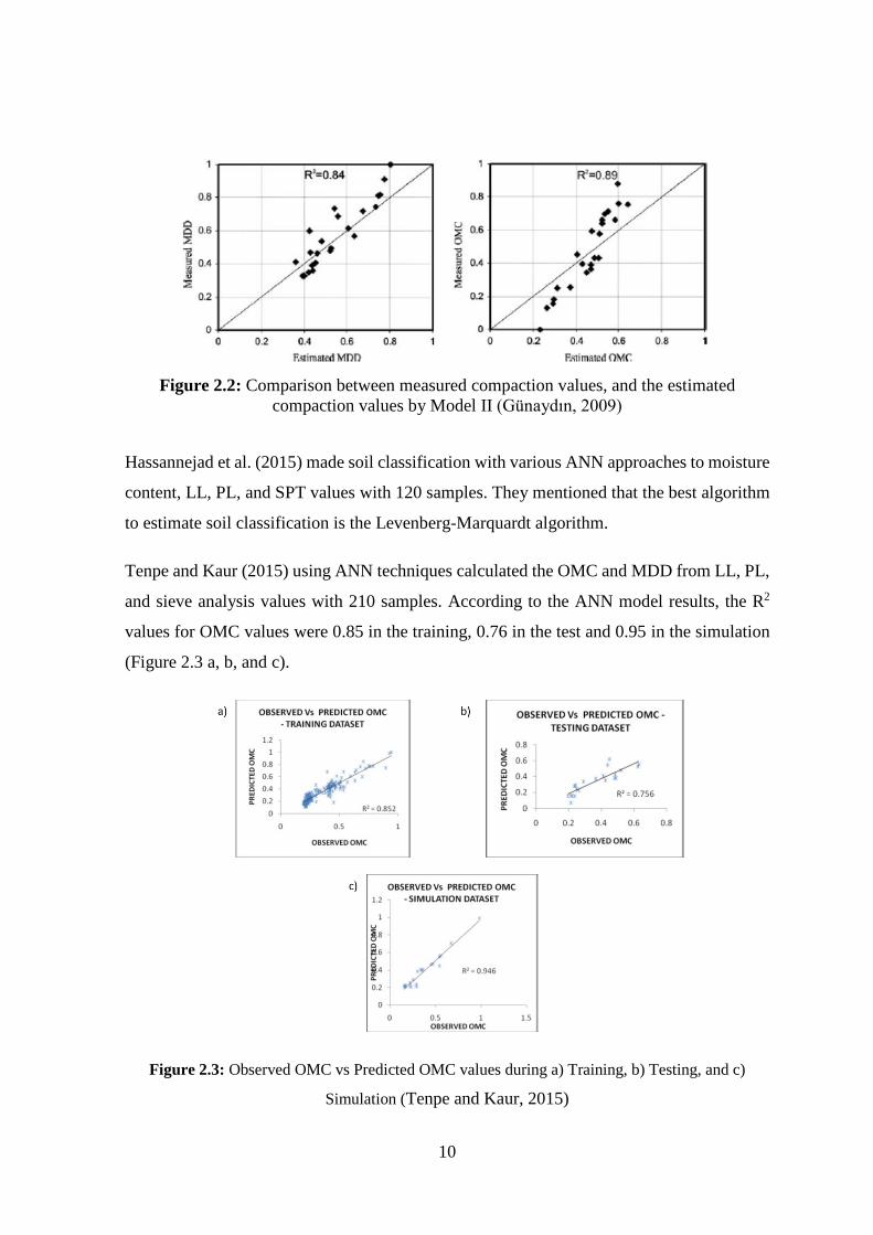
10
Figure 2.2: Comparison between measured compaction values, and the estimated
compaction values by Model II (Günaydın, 2009)
Hassannejad et al. (2015) made soil classification with various ANN approaches to moisture
content, LL, PL, and SPT values with 120 samples. They mentioned that the best algorithm
to estimate soil classification is the Levenberg-Marquardt algorithm.
Tenpe and Kaur (2015) using ANN techniques calculated the OMC and MDD from LL, PL,
and sieve analysis values with 210 samples. According to the ANN model results, the R2
values for OMC values were 0.85 in the training, 0.76 in the test and 0.95 in the simulation
(Figure 2.3 a, b, and c).
Figure 2.3: Observed OMC vs Predicted OMC values during a) Training, b) Testing, and c)
Simulation (Tenpe and Kaur, 2015)
Page 26
11
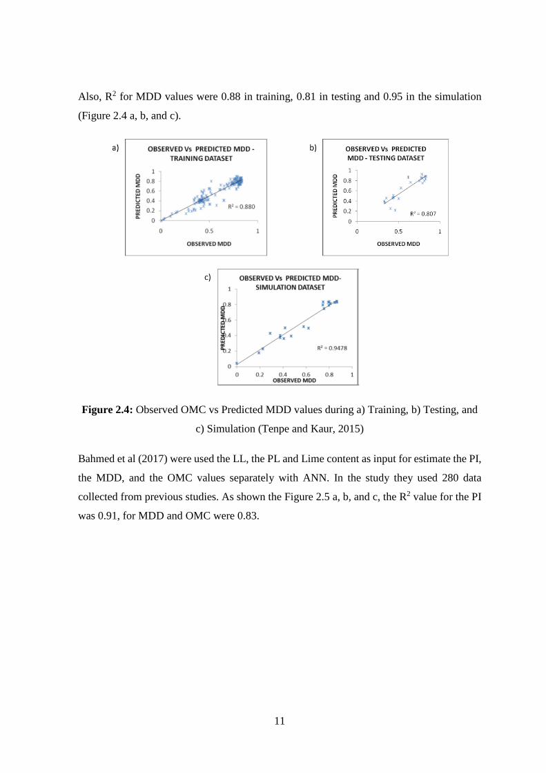
Also, R2 for MDD values were 0.88 in training, 0.81 in testing and 0.95 in the simulation
(Figure 2.4 a, b, and c).
Figure 2.4: Observed OMC vs Predicted MDD values during a) Training, b) Testing, and
c) Simulation (Tenpe and Kaur, 2015)
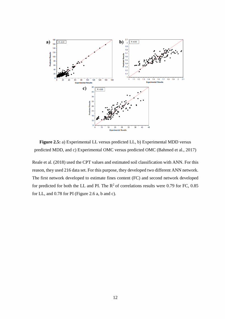
Bahmed et al (2017) were used the LL, the PL and Lime content as input for estimate the PI,
the MDD, and the OMC values separately with ANN. In the study they used 280 data
collected from previous studies. As shown the Figure 2.5 a, b, and c, the R2 value for the PI
was 0.91, for MDD and OMC were 0.83.
Page 27
12
Figure 2.5: a) Experimental LL versus predicted LL, b) Experimental MDD versus
predicted MDD, and c) Experimental OMC versus predicted OMC (Bahmed et al., 2017)
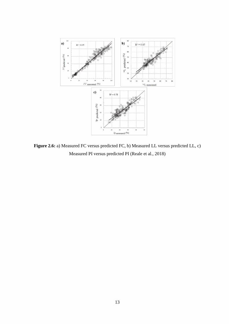
Reale et al. (2018) used the CPT values and estimated soil classification with ANN. For this
reason, they used 216 data set. For this purpose, they developed two different ANN network.
The first network developed to estimate fines content (FC) and second network developed
for predicted for both the LL and PI. The R2 of correlations results were 0.79 for FC, 0.85
for LL, and 0.78 for PI (Figure 2.6 a, b and c).
Page 28
13
Figure 2.6: a) Measured FC versus predicted FC, b) Measured LL versus predicted LL, c)
Measured PI versus predicted PI (Reale et al., 2018)
Page 29
14
CHAPTER 3
MATERIALS AND METHODS
3.1. Area of Study
The soil samples and data used in this project were collected from various parts of Cyprus,
especially Nicosia. The samples represent the different depth and soil types. The island of
Cyprus is the third of the Mediterranean and the largest island of the Eastern Mediterranean
with an area of 9251 km2. The total area of North Cyprus is 3299 km2.
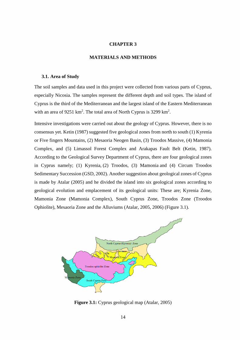
Intensive investigations were carried out about the geology of Cyprus. However, there is no
consensus yet. Ketin (1987) suggested five geological zones from north to south (1) Kyrenia
or Five fingers Mountains, (2) Mesaoria Neogen Basin, (3) Troodos Massive, (4) Mamonia
Complex, and (5) Limassol Forest Complex and Arakapas Fault Belt (Ketin, 1987).
According to the Geological Survey Department of Cyprus, there are four geological zones
in Cyprus namely; (1) Kyrenia, (2) Troodos, (3) Mamonia and (4) Circum Troodos
Sedimentary Succession (GSD, 2002). Another suggestion about geological zones of Cyprus
is made by Atalar (2005) and he divided the island into six geological zones according to
geological evolution and emplacement of its geological units: These are; Kyrenia Zone,
Mamonia Zone (Mamonia Complex), South Cyprus Zone, Troodos Zone (Troodos
Ophiolite), Mesaoria Zone and the Alluviums (Atalar, 2005, 2006) (Figure 3.1).
Figure 3.1: Cyprus geological map (Atalar, 2005)
Page 30
15
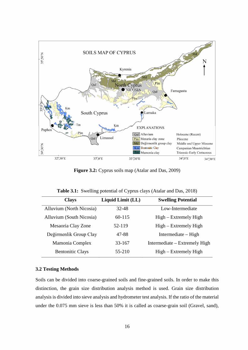
The majority of the Cyprus soils are alluviums and over-consolidated clays (Table 3.1). The
alluviums are located between the Kyrenia and Trodos mountain ranges, which are flat and
topographically low areas. These represent the soils in the center of Cyprus (Atalar and Das,
2009). Alluvial soils consist of loose-medium density gravel and sand and soft hard silt and
clays. The clay size amount in the alluviums is low. The amount of montmorillonite in the
alluvium is high. These alluviums have partially high strength when dry. However, their
strength is reduced with saturation. These clayey soils have low to intermediate swelling
potential in North Cyprus. They were observed especially on the east and west coasts within
the old harbors. There are old river beds filled with alluviums on the shoreline and inland.
Mesaoria clay zone; consists of clay with high and very high swelling potential. This group,
which is heavily observed in the middle of the Island, have high and extremely high swelling
potential (Table 3.1) especially in Nicosia, Famagusta, Larnaca, and Polis. This zone, which
is mainly composed marl, also contains calcaremite, conglomerates, limestone, and gravel.
Clays of Değirmenlik (Kythrea) Group; This group includes mostly turbidite rocks. The
group consists of gravel, pebbles, greywacke, marl and abyssal turbidites with mostly
shallow environmental limestone, chalk, marl, limestone, and gypsum. The tens of meters
of clayey units, which are several meters thick in different formations of the Değirmenlik
(Kythrea) group, exhibit varied swelling potential. Haspolat (Mia Milia) present
intermediate to high swelling potential, Yılmazköy (Skylloura) and Yazılıtepe (Lapatza)
formations present high to very high swelling potential (Atalar, 2004).
Bentonitic Clays are formed by pillow lavas (Troodos Ophiolites) and form the first clays of
Cyprus. Reaches a thickness of more than 300 meters in South Cyprus. Although 35% of
bentonitic clays are calcium montmorillonite with low swelling potential, bentonitic clays
have the highest swelling potential of Cyprus clays.
Clays of Momonia Complex are within igneous-volcanic, and metamorphic rocks of the
Mamonia Complex of Middle Triassic to Cretaceous ages. Their swelling potential is much
less than in the bentonitic clays (Figure 3.2).
Page 31
16
Figure 3.2: Cyprus soils map (Atalar and Das, 2009)
Table 3.1: Swelling potential of Cyprus clays (Atalar and Das, 2018)
Clays Liquid Limit (LL) Swelling Potential
Alluvium (North Nicosia) 32-48 Low-Intermediate
Alluvium (South Nicosia) 60-115 High – Extremely High
Mesaoria Clay Zone 52-119 High – Extremely High
Değirmenlik Group Clay 47-88 Intermediate – High
Mamonia Complex 33-167 Intermediate – Extremely High
Bentonitic Clays 55-210 High – Extremely High
3.2 Testing Methods
Soils can be divided into coarse-grained soils and fine-grained soils. In order to make this
distinction, the grain size distribution analysis method is used. Grain size distribution
analysis is divided into sieve analysis and hydrometer test analysis. If the ratio of the material
under the 0.075 mm sieve is less than 50% it is called as coarse-grain soil (Gravel, sand),
Page 32
17
and if it is more than 50%, it is called as fine-grained soil (silt, clay). Fine-grained soils are
determined by hydrometer analysis after sieve analysis. We need LL and PI values when
classifying fine-grained soils. Atterberg limit tests are performed for this purpose.
3.2.1. Grain size distribution
Grain Size Distribution analysis can be defined as the combination of two methods; sieve
analysis and hydrometer analysis.
a) Sieve Analysis Test
During the analysis of the field works, reports, and projects sieve analysis were performing
by using appropriate sieves according to ASTM D6913-17 standards. Samples were dried
overnight at 105 ° C to 110 ° C. After the samples were cooled, they took to the sieve and
the sieving process is performed. In the process using sieves with different sizes, the amount
of sample remaining after each sieve is noted.
b) Hydrometer Test
In accordance with ASTM D 422-63 - Standard Test Method for Particle-Size Analysis of
Soils standards;
• Samples remaining in the tray after sieve analysis are used for hydrometer analysis.
Dispersing agents (Sodium Hexametaphosphate (40 g / L)) is added to the clay and
silt grains to prevent them from sticking together and are allowed to soak for 10
minutes.
• The prepared solution is taken up in the precipitation vessel and pure water is added
until the volume of the solution is reached.
• The open-end vessel is sealed with a stopper and upend 30 times per minute.
• After the vessel is directed, the cover is removed and time is recorded. After 1 minute
40 seconds the hydrometer is placed in the cylinder for the first reading.
• An identical 1000 ml vessel is filled with distilled water and the hydrometer is
calibrated. Hydrometer reading in distilled water should normally be zero. A reading
other than that is recorded and used as a hydrometer correction.
Page 33
18
• For the first reading of the suspension, the hydrometer is slowly released into the
liquid and the value is recorded.
• In the hydrometer test, readings are performed after 30 seconds, 1, 2, 4, 8, 15, 30, 60,
120, 240 and 1440 minutes.
• At each reading, the temperature of the suspension liquid is recorded and after
reading, the hydrometer is swirled inside the control vessel.
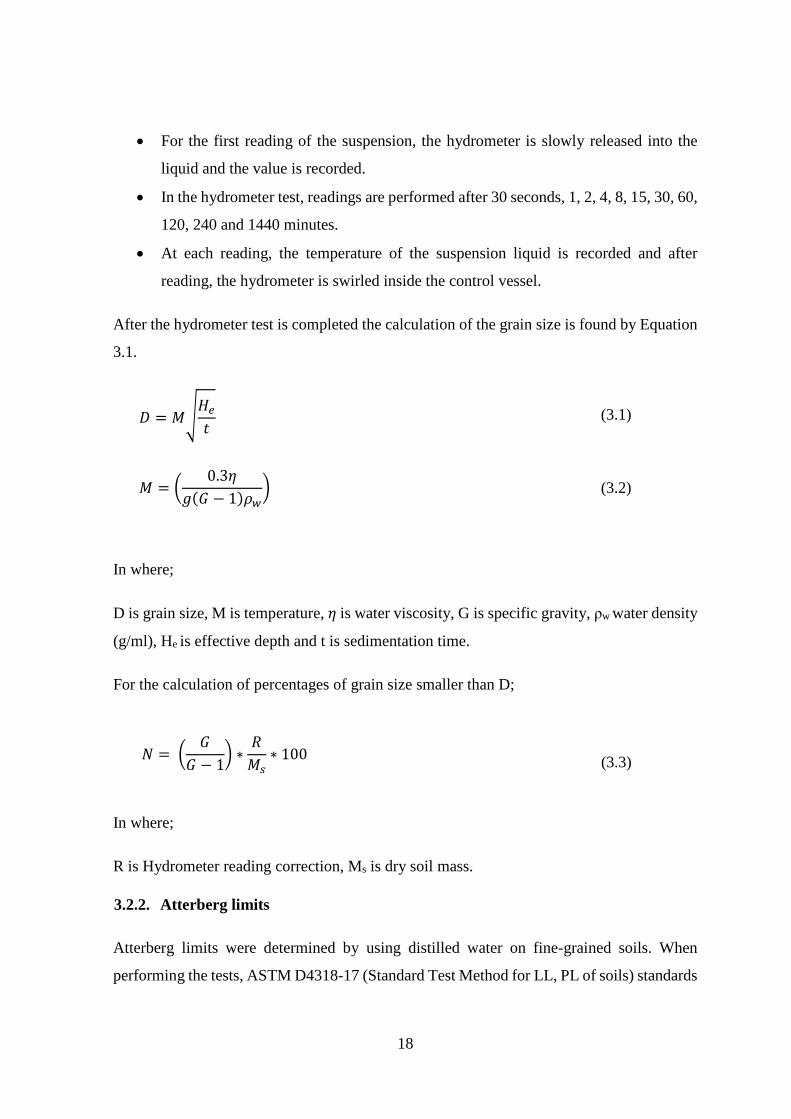
After the hydrometer test is completed the calculation of the grain size is found by Equation
3.1.
𝐷𝐷 = 𝑂𝑂�𝐻𝐻𝑒𝑒𝑡𝑡
(3.1)
𝑂𝑂 = �0.3𝜂𝜂
𝑔𝑔(𝐺𝐺 − 1)𝜌𝜌𝑤𝑤� (3.2)
In where;
D is grain size, M is temperature, 𝜂𝜂 is water viscosity, G is specific gravity, ρw water density
(g/ml), He is effective depth and t is sedimentation time.
For the calculation of percentages of grain size smaller than D;
In where;
R is Hydrometer reading correction, Ms is dry soil mass.
3.2.2. Atterberg limits
Atterberg limits were determined by using distilled water on fine-grained soils. When
performing the tests, ASTM D4318-17 (Standard Test Method for LL, PL of soils) standards
𝑁𝑁 = �𝐺𝐺
𝐺𝐺 − 1� ∗
𝑅𝑅𝑂𝑂𝑠𝑠
∗ 100 (3.3)
Page 34
19
are followed. The tests are performed with 200 gr soil sample which passes from No.40
(0.425 mm) sieve.
3.3 Artificial Neural Network
3.3.1. Definition of ANN
The basis of the ANNs began in 1942 with the first cell model proposed by McCulloch and Pitts.
An ANN is a complex neural network composed of a combination of many simple nerve
cells (Lippmann, 1987). Important features of ANNs are solving non-linear problems,
having a distributed parallel structure, learning, error tolerance, and generalization. Through
to these features are used in many areas. One of the important features of ANNs is learning
and generalize this learning. By exploring the relationship between inputs and outputs given
to the network, it is able to produce the appropriate outputs against unrecognized data (Garip,
2011).
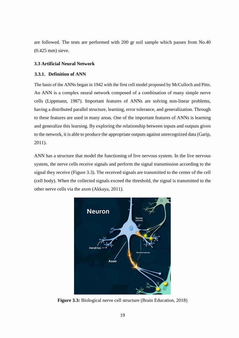
ANN has a structure that model the functioning of live nervous system. In the live nervous
system, the nerve cells receive signals and perform the signal transmission according to the
signal they receive (Figure 3.3). The received signals are transmitted to the center of the cell
(cell body). When the collected signals exceed the threshold, the signal is transmitted to the
other nerve cells via the axon (Akkaya, 2011).
Figure 3.3: Biological nerve cell structure (Brain Education, 2018)
Page 35
20
ANN is formed by the combination of many artificial nerve cells. This combination takes
place in layers, not arbitrary (Akkaya, 2011).
We can mention about 3 learning strategies used in ANN.
a) Supervised Learning: Supervised learning is a machine learning technique that
produces a function through training data. In other words, in this learning technique,
the algorithm generates a function that makes a matching function between inputs
and outputs (Hinton et al., 1999).
b) Unsupervised Learning: Unsupervised Learning model is a machine learning
technique based on observations. In other words, the method tries to perform learning
only through inputs without using output data. This method is especially used to
collect the data set (Hinton et al., 1999).
c) Reinforcement Learning: Reinforcement Learning, a type of machine learning,
demonstrates how an autonomous agent who senses the environment in which it is
located and learns to make the right decisions to reach its goal (Johnson et al., 2000).
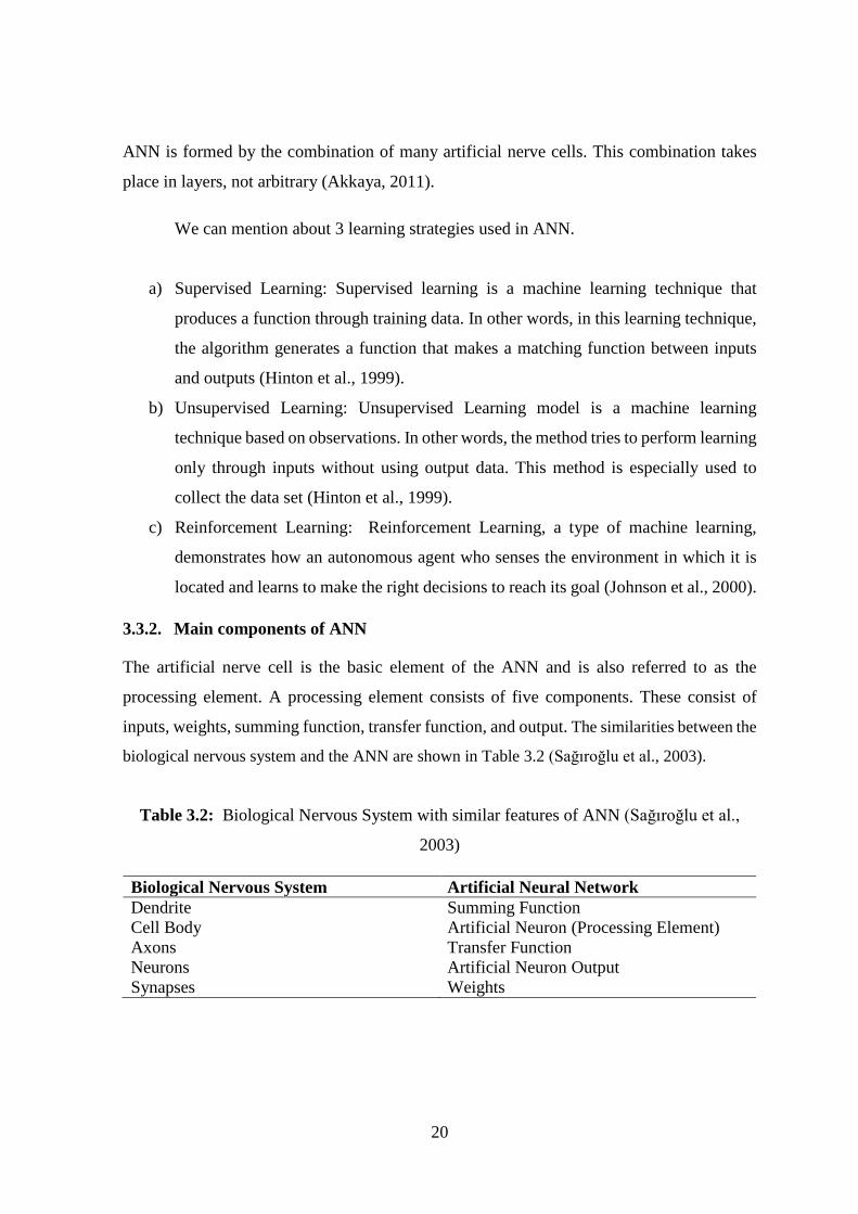
3.3.2. Main components of ANN
The artificial nerve cell is the basic element of the ANN and is also referred to as the
processing element. A processing element consists of five components. These consist of
inputs, weights, summing function, transfer function, and output. The similarities between the
biological nervous system and the ANN are shown in Table 3.2 (Sağıroğlu et al., 2003).
Table 3.2: Biological Nervous System with similar features of ANN (Sağıroğlu et al.,
2003)
Biological Nervous System Artificial Neural Network Dendrite Summing Function Cell Body Artificial Neuron (Processing Element) Axons Transfer Function Neurons Artificial Neuron Output Synapses Weights
Page 36
21
3.3.2.1. Inputs
The inputs are data from outside a neuron, and these data may come from an external neuron
or neuron itself to the neuron (Aslay and Üstün, 2013). The basis of network training is input.
3.3.2.2. Weights
The weights are represented by w coefficients showing the effect of input data from the
neural nerve on the nerve cell. Each input has a weight. The high weight value indicates that
the input is important and the effective rate is high. Low weight values indicate that input is
insignificant (Elmas, 2007). Weights are used in the relationship between input and output
values (Garip, 2011).
3.3.2.3. Summing function
It calculates the net input from the neuron and different functions can be used to perform
this calculation. The most commonly used method is the weighted sum (Hamzaçebi, 2011).
The summing function equation is shown in Equation 3.4.
𝑉𝑉𝑘𝑘 = �𝑥𝑥𝑖𝑖𝑤𝑤𝑘𝑘𝑖𝑖
𝑛𝑛
𝑖𝑖=1
(3.4)
In equation 3.4; 𝑉𝑉𝑘𝑘 is net input, 𝑥𝑥𝑖𝑖 is ANNs input values, 𝑤𝑤𝑘𝑘𝑖𝑖 is weights (i. input range k.
neuron connecting weight), n is number of inputs. The selection of the summing function
may vary depending on the problem. The trial and error method is used for the determination
of ideal summing function.
3.3.2.4 Activation function
It is the function that keeps the output value against the net input value of the neuron in a certain
range. It establishes a bond between the input and output values of the neuron (Haykin and
Network, 2004). It processes the total input to the cell and generates the corresponding output. Different functions are used for output generating. Some network models require the use of a
derivative function (Öztemel, 2003).
Page 37
22
The activation function may be of different types depending on the function of the neuron. The
optimal activation function can be found as a result of the attempts of the network developer, the
activation functions can be fixed or adaptable. The most frequently used activation functions are
sigmoid and hyperbolic tangent functions (Kakıcı, 2017).
a) Sigmoid Function (logsig): The sigmoid activation function is a continuous and
derivative function. It is one of the most frequently used functions in ANN
applications due to its non-linearity. This function generates a value between zero
and one for each of the input values. The input-output expression of this activation
function and the change of the function relative to the input are given respectively in
Equation 3.5 and in Figure 3.4.
𝑎𝑎 =1
1 + 𝑒𝑒−𝑛𝑛 (3.5)
Figure 3.4: Sigmoid activation function
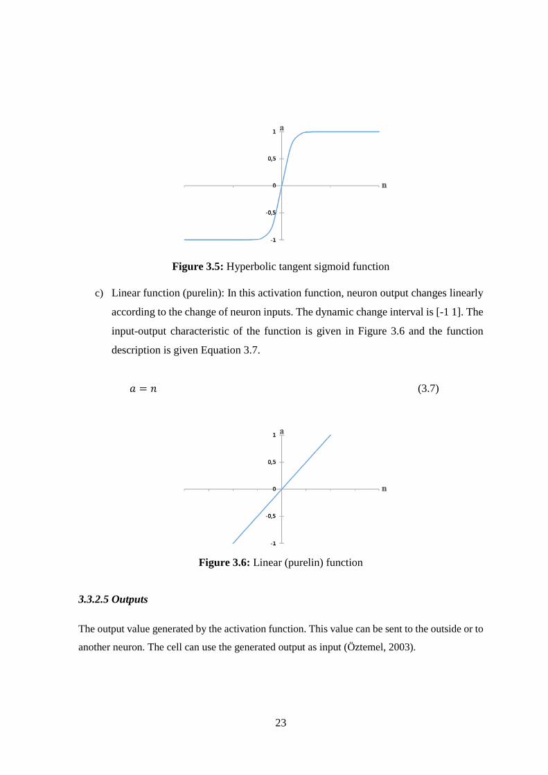
b) Hyperbolic tangent sigmoid function (tansig): For this activation function, the neuron
input-output expression is given Equation 3.6 and the change of function are given
in Figure 3.5. The dynamic change interval of the function is the range [-1 1] and the
function shows a non-linear change in this range depending on the total input of the
neuron.
𝑎𝑎 = 𝑒𝑒𝑛𝑛 − 𝑒𝑒−𝑛𝑛
𝑒𝑒𝑛𝑛 + 𝑒𝑒−𝑛𝑛 (3.6)
Page 38
23
Figure 3.5: Hyperbolic tangent sigmoid function
c) Linear function (purelin): In this activation function, neuron output changes linearly
according to the change of neuron inputs. The dynamic change interval is [-1 1]. The
input-output characteristic of the function is given in Figure 3.6 and the function
description is given Equation 3.7.
𝑎𝑎 = 𝑛𝑛 (3.7)
Figure 3.6: Linear (purelin) function
3.3.2.5 Outputs
The output value generated by the activation function. This value can be sent to the outside or to
another neuron. The cell can use the generated output as input (Öztemel, 2003).
Page 39
24
3.3.3. Neural network types
There are many different types of ANN, such as;
• Adaptive Resonance Theory (ART) Network
• Backpropagation networks
• Radial Basis Function (RBF) Network
• Kohonen Network
• Hopfield Network
• Recurrent Neural Networks (RNN)
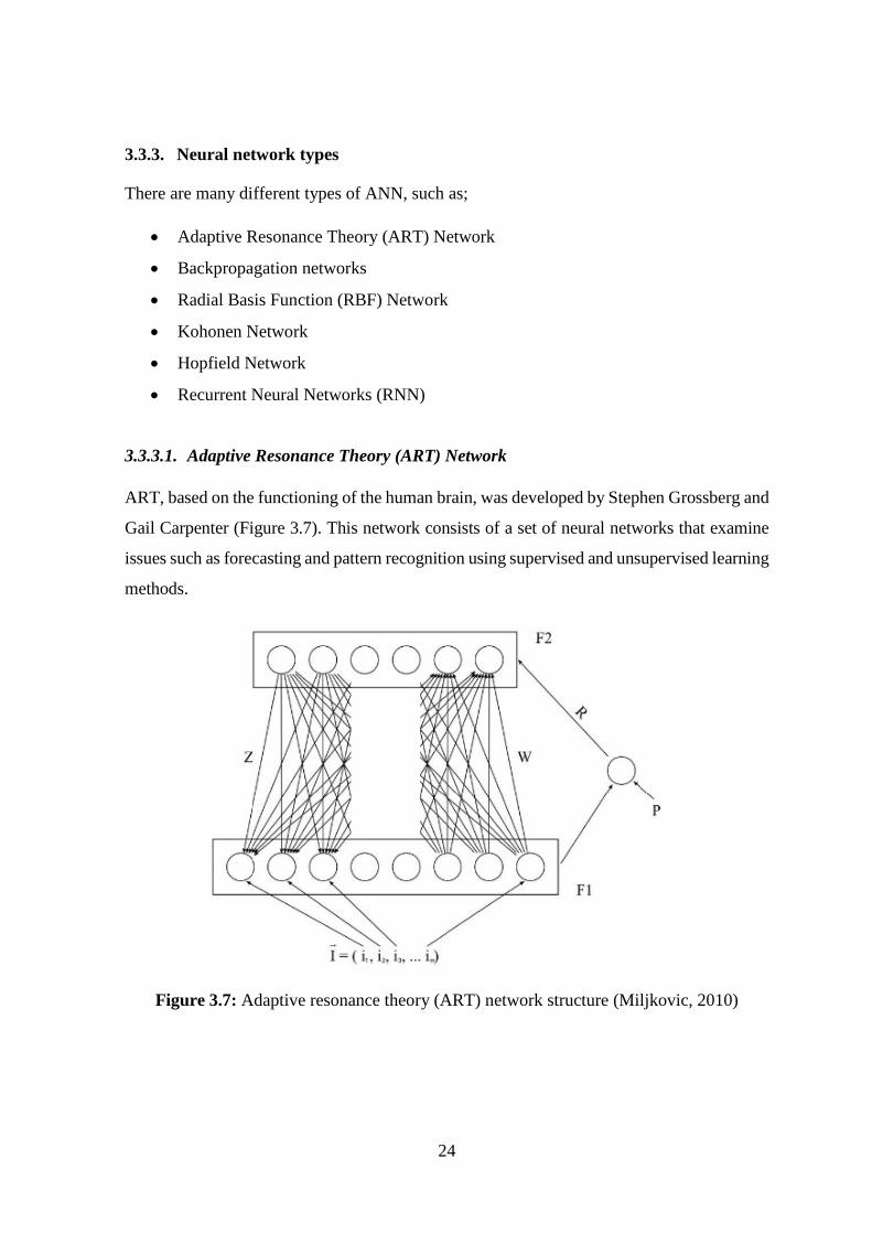
3.3.3.1. Adaptive Resonance Theory (ART) Network
ART, based on the functioning of the human brain, was developed by Stephen Grossberg and
Gail Carpenter (Figure 3.7). This network consists of a set of neural networks that examine
issues such as forecasting and pattern recognition using supervised and unsupervised learning
methods.
Figure 3.7: Adaptive resonance theory (ART) network structure (Miljkovic, 2010)
Page 40
25
The basis of the network is the search for the presented model for a match in the stored
categories. If this searching is not giving any matching, the network considers this model as
an innovation.
3.3.3.2. Backpropagation networks
Backpropagation network is one of the most used artificial neural network models in
engineering applications. The main principle of the Backpropagation network is to minimize
the error obtained at the output of the selected network structure and to accordingly change
the network weights. In this type of ANN, the processing elements (neurons) are arranged
in layers. Each network model consists of at least three layers as input, hidden layer and
output.
The backpropagation network model consists of seven learning steps, the first four of which
are forward, and the last three steps are backward steps.
1. Defining the network structure: The number of inputs, output, a hidden layer, and
neuron numbers is determined.
2. Determination of initial network parameters: The weight and bias to be used in the
selected network structure are determined.
3. Identification the learning set to the network: A learning set consisting of inputs and
outputs to be used to solve the problem or application is identified to the network.
4. Presence the last output of the network: For each processing element used in the
network architecture, the total input, and transfer values are calculated and the last
output of the network is the presence.
5. The error between the original value and the network output value is calculated.
6. The error is distributed to backward weights, starting from the output layer.
7. If the error is within acceptable limits, the operation is stopped, otherwise is returned
to step 3.
The backpropagation network model tries to reach to minimum error value by increasing
or decreasing the weight value it assigns after each approach. It is difficult to estimate the
weight values to be used between input and output parameters. The advantage of the
system are that the network propagation backwards and changes the weights according to
Page 41
26
the error rate. As in this study, backpropagation network model is preferred for problems
that do not have a linear relationship between input and output parameters.
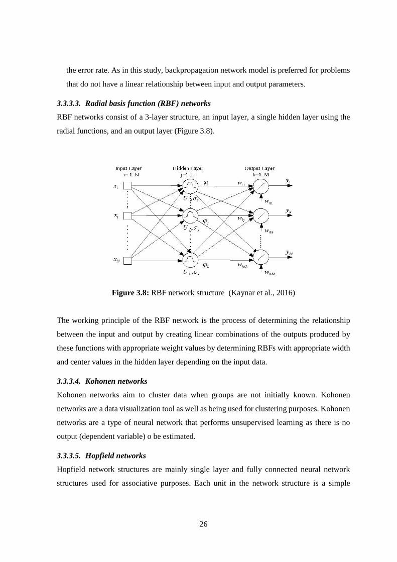
3.3.3.3. Radial basis function (RBF) networks
RBF networks consist of a 3-layer structure, an input layer, a single hidden layer using the
radial functions, and an output layer (Figure 3.8).
Figure 3.8: RBF network structure (Kaynar et al., 2016)
The working principle of the RBF network is the process of determining the relationship
between the input and output by creating linear combinations of the outputs produced by
these functions with appropriate weight values by determining RBFs with appropriate width
and center values in the hidden layer depending on the input data.
3.3.3.4. Kohonen networks
Kohonen networks aim to cluster data when groups are not initially known. Kohonen
networks are a data visualization tool as well as being used for clustering purposes. Kohonen
networks are a type of neural network that performs unsupervised learning as there is no
output (dependent variable) o be estimated.
3.3.3.5. Hopfield networks
Hopfield network structures are mainly single layer and fully connected neural network
structures used for associative purposes. Each unit in the network structure is a simple
Page 42
27
threshold value processor unit and there is a bi-directional connection weighted between
each processor unit pair.
3.3.3.6. Recurrent networks
The Recurrent Neural Network (RNN) is an artificial neural network model where the links
between the units form a directed loop. With this loop, a network internal state has been
created that allows it to display dynamic temporal behavior. In contrast to feed-forward
neural networks, RNNs can use their input memory to process random sequences of inputs
(Mikolov, 2010).
Page 43
28
CHAPTER 4
DATA ANALYSIS AND RESULTS
A kind of different approaches can be used to provide the relationship between the
multivariate data. As a classical method, multivariate regression coefficient estimates can be
used. Besides, in these days’ ANN are used as an alternative way to this method. This thesis
includes 108 data from field works and previous reports, and projects such as Swelling Clay
Project (Atalar, 2002; Geotest, 2014; Hussain 2016). These data are compiled according to
grain size distribution (% sand, % silt, % clay) and Atterberg limit values. The main aim of
this thesis is to predict soil classification with grain size distribution analysis by using ANN.
Therefore, at the first phase of this study we predicted liquid limit and plasticity index from
grain size distribution with ANN, and in the second phase, we determined soil classification
from the Unified Soil Classification System (USCS) chart.
4.1. Data Analysis Methods
There are many methods used to determine the relationship between variables. However, in
this study, multiple linear regression and artificial neural network training algorithm
methods were used. The coefficient of determination is used as a parameter to determine the
degree of accuracy of these methods. If it is necessary to explain this; Coefficient of
determination (R2) is shown in Equation 4.1;
𝑅𝑅2 = 1 −𝑆𝑆𝑆𝑆𝑆𝑆𝑆𝑆𝑆𝑆𝑆𝑆
(4.1)
Where; SSE (Equation 4.2) is the sum of squares of model errors and SST (Equation 4.3) is
the square sum of the errors in the model.
𝑆𝑆𝑆𝑆𝑆𝑆 = �(𝑦𝑦𝑖𝑖 − 𝑦𝑦𝚤𝚤�)2𝑛𝑛
𝑖𝑖=1
(4.2)
Page 44
29
𝑆𝑆𝑆𝑆𝑆𝑆 = �(𝑦𝑦𝑖𝑖 − 𝑦𝑦�)2𝑛𝑛
𝑖𝑖=1
(4.3)
It is one of the most important parameters used in observing the correspondence between
estimated values and actual values. R2 values descriptive between 0 and +1. Chin (1998)
described the accuracy level of R2 like substantial, more moderate, and weak (Table 4.1).
Table 4.1: Accuracy of coefficient determination (Chin, 1998)
R2 Desired Value
0.67 Substantial
0.33 More Moderate
0.19 Weak
Data normalization (Equation 4.4) has been applied in order to calculate the predicted values
in a healthy and secure way. There are differences between the input and output parameter
values. This process was applied to group the data in a certain order and range (between 0
and 1). Another benefit of this process is to reduce the processing time. Is shown in Equation
4.4.
𝑋𝑋′ =𝑋𝑋 − 𝑋𝑋𝑚𝑚𝑖𝑖𝑛𝑛
𝑋𝑋𝑚𝑚𝑚𝑚𝑚𝑚 − 𝑋𝑋𝑚𝑚𝑖𝑖𝑛𝑛 (4.4)
4.2. Multiple Linear Regression Analysis
Multiple linear regression is the analysis of being able to explain the relationship between a
single dependent variable and multiple independent variables (Equation 4.5). There is a
correlation between the dependent and independent variables in this analysis method.
Page 45
30
The most general regression equation;
𝑌𝑌 = 𝑎𝑎0 + 𝑎𝑎1𝑋𝑋1 + 𝑎𝑎2𝑋𝑋2 + ⋯+ 𝑎𝑎𝑛𝑛𝑋𝑋𝑛𝑛 + 𝑒𝑒𝑖𝑖 (4.5)
Where; Xi are independent, Yi dependent variables and ei is error term (Y-Ŷ).
In this study, sand, silt, clay percentages were used as independent variables. Liquid limit
and plasticity index were evaluated separately as dependent variables. In Table 4.2 is shown
that statistical properties of the data.
Table 4.2: Data properties
% Sand % Silt % Clay LL PI
Min 0.4 8.7 25.3 26.3 5.1
Max 49.7 51.7 78.0 87.5 56.7
Std. Dev. 12.98 9.55 12.37 15.05 13.81
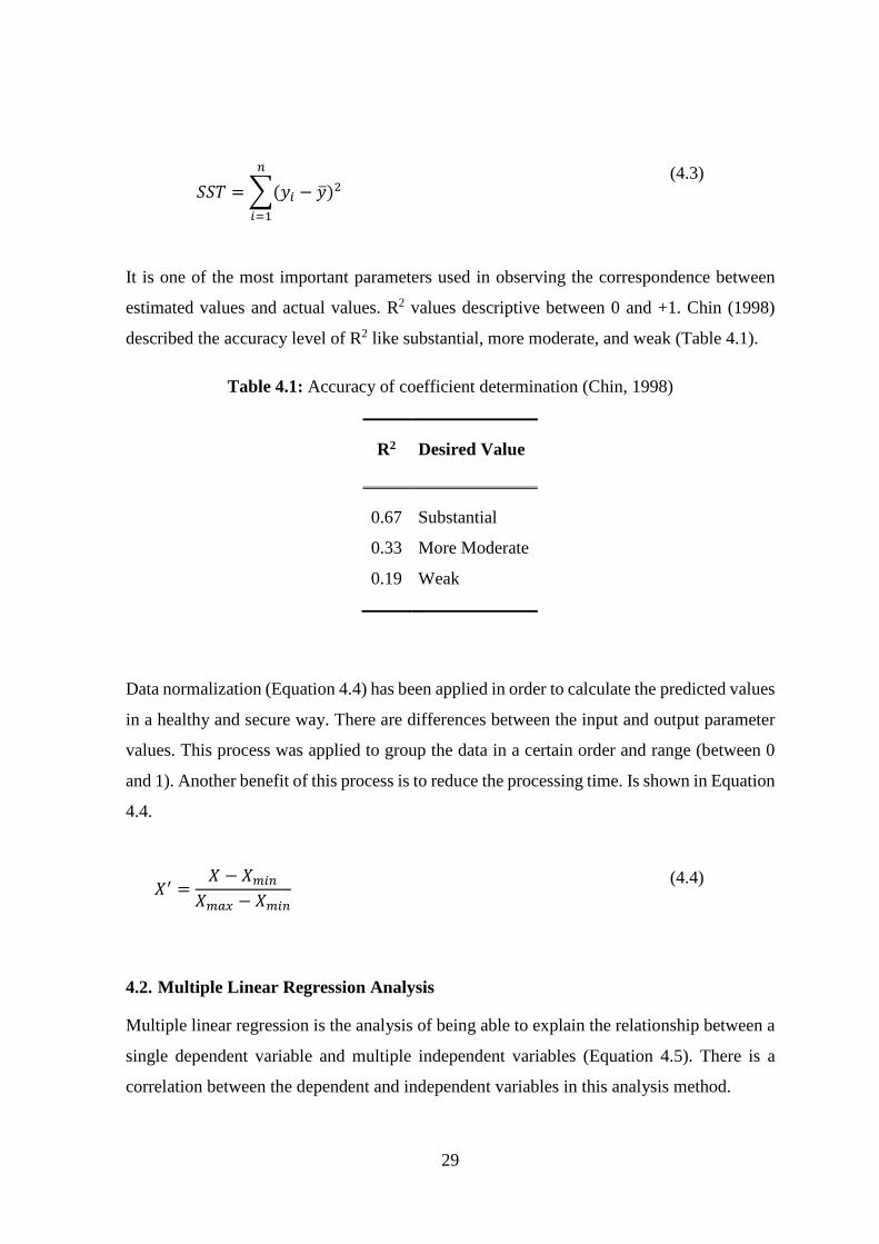
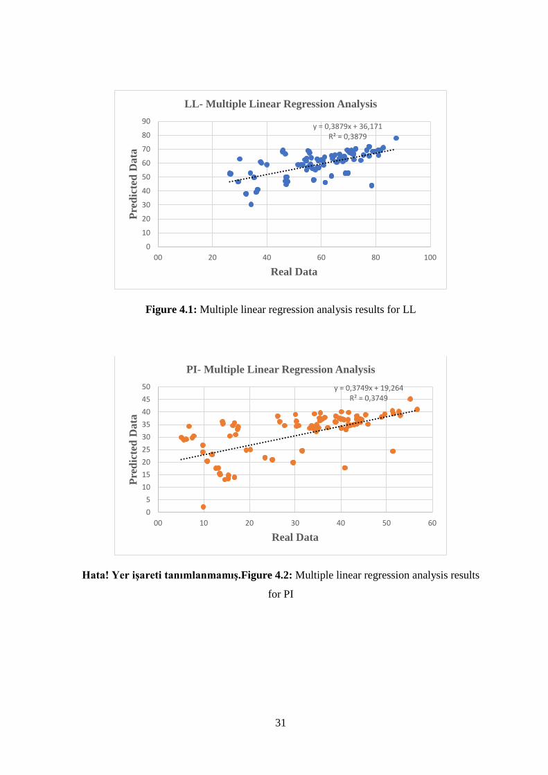
As is shown in Table 4.3 R2 values are about 0.38. The comparisons of multiple regression
analysis results are shown in Figure 4.1 for LL and Figure 4.2 for PI. That’s mean the
accuracy of variables being more moderate. This isn’t enough for us. Due to this reason, we
can’t trust this analysis result. In cases where multiple regression analysis is inadequate, the
ANN method is used as an alternative method.
Table 4.3: Multiple linear regression analysis results
Dependent
Variables
Independent Variables 𝒂𝒂𝟎𝟎 R2
%Sand %Silt %Clay
LL 7.184287 6.890024 7.788753 -683.325 0.387924
PI 7.198396 6.645002 7.507712 -690.861 0.374896
Page 46
31
Figure 4.1: Multiple linear regression analysis results for LL
Hata! Yer işareti tanımlanmamış.Figure 4.2: Multiple linear regression analysis results
for PI
y = 0,3879x + 36,171R² = 0,3879
0
10
20
30
40
50
60
70
80
90
00 20 40 60 80 100
Pred
icte
d D
ata
Real Data
LL- Multiple Linear Regression Analysis
y = 0,3749x + 19,264R² = 0,3749
05
101520253035404550
00 10 20 30 40 50 60
Pred
icte
d D
ata
Real Data
PI- Multiple Linear Regression Analysis
Page 47
32
4.3. Artificial Neural Network Training Algorithm
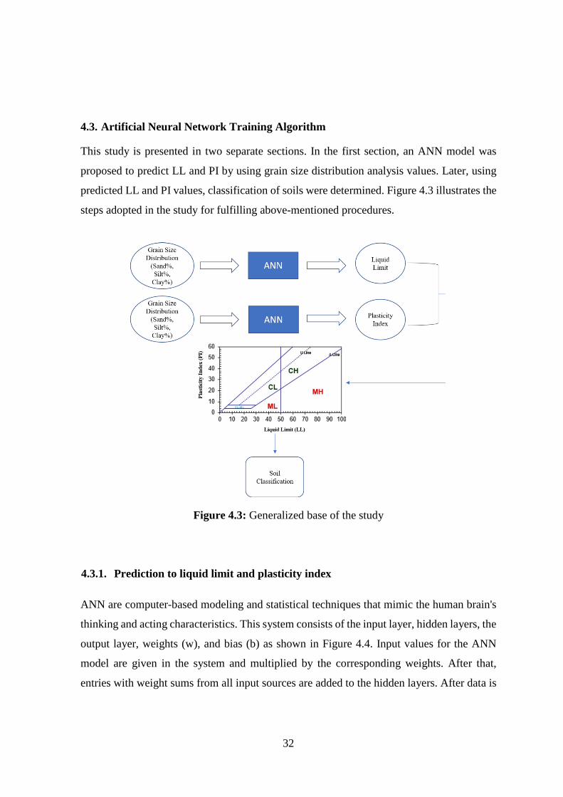
This study is presented in two separate sections. In the first section, an ANN model was
proposed to predict LL and PI by using grain size distribution analysis values. Later, using
predicted LL and PI values, classification of soils were determined. Figure 4.3 illustrates the
steps adopted in the study for fulfilling above-mentioned procedures.
Figure 4.3: Generalized base of the study
4.3.1. Prediction to liquid limit and plasticity index
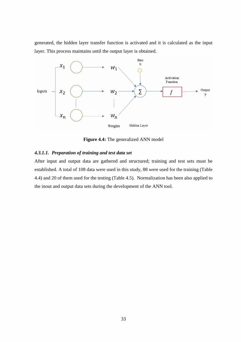
ANN are computer-based modeling and statistical techniques that mimic the human brain's
thinking and acting characteristics. This system consists of the input layer, hidden layers, the
output layer, weights (w), and bias (b) as shown in Figure 4.4. Input values for the ANN
model are given in the system and multiplied by the corresponding weights. After that,
entries with weight sums from all input sources are added to the hidden layers. After data is
Page 48
33
generated, the hidden layer transfer function is activated and it is calculated as the input
layer. This process maintains until the output layer is obtained.
Figure 4.4: The generalized ANN model
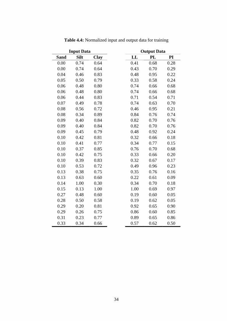
4.3.1.1. Preparation of training and test data set
After input and output data are gathered and structured; training and test sets must be
established. A total of 108 data were used in this study, 88 were used for the training (Table
4.4) and 20 of them used for the testing (Table 4.5). Normalization has been also applied to
the inout and output data sets during the development of the ANN tool.
Page 49
34
Table 4.4: Normalized input and output data for training
Input Data Output Data Sand Silt Clay LL PL PI 0.00 0.74 0.64 0.41 0.68 0.28 0.00 0.74 0.64 0.43 0.70 0.29 0.04 0.46 0.83 0.48 0.95 0.22 0.05 0.50 0.79 0.33 0.58 0.24 0.06 0.48 0.80 0.74 0.66 0.68 0.06 0.48 0.80 0.74 0.66 0.68 0.06 0.44 0.83 0.71 0.54 0.71 0.07 0.49 0.78 0.74 0.63 0.70 0.08 0.56 0.72 0.46 0.95 0.21 0.08 0.34 0.89 0.84 0.76 0.74 0.09 0.40 0.84 0.82 0.70 0.76 0.09 0.40 0.84 0.82 0.70 0.76 0.09 0.45 0.79 0.48 0.92 0.24 0.10 0.42 0.81 0.32 0.66 0.18 0.10 0.41 0.77 0.34 0.77 0.15 0.10 0.37 0.85 0.76 0.70 0.68 0.10 0.42 0.75 0.33 0.66 0.20 0.10 0.39 0.83 0.32 0.67 0.17 0.10 0.53 0.72 0.49 0.96 0.23 0.13 0.38 0.75 0.35 0.76 0.16 0.13 0.63 0.60 0.22 0.61 0.09 0.14 1.00 0.30 0.34 0.70 0.18 0.15 0.13 1.00 1.00 0.69 0.97 0.27 0.48 0.60 0.19 0.60 0.05 0.28 0.50 0.58 0.19 0.62 0.05 0.29 0.20 0.81 0.92 0.65 0.90 0.29 0.26 0.75 0.86 0.60 0.85 0.31 0.23 0.77 0.89 0.65 0.86 0.33 0.34 0.66 0.57 0.62 0.50
Page 50
35
Table 4.4 Continued
Input Data Output Data Sand Silt Clay LL PL PI 0.34 0.21 0.75 0.91 0.62 0.90 0.35 0.22 0.73 0.87 0.47 0.93 0.36 0.19 0.75 0.71 0.52 0.71 0.36 0.55 0.39 0.13 0.38 0.09 0.36 0.67 0.36 0.61 1.00 0.35 0.37 0.61 0.40 0.12 0.38 0.09 0.38 0.28 0.66 0.84 0.73 0.76 0.39 0.59 0.40 0.71 0.16 0.90 0.39 0.59 0.40 0.71 0.16 0.90 0.40 0.21 0.70 0.74 0.70 0.66 0.41 0.16 0.73 0.73 0.15 0.92 0.41 0.32 0.60 0.06 0.34 0.03 0.42 0.33 0.59 0.69 0.65 0.62 0.42 0.24 0.66 0.80 0.64 0.76 0.42 0.58 0.38 0.70 0.89 0.51 0.42 0.58 0.38 0.70 0.89 0.51 0.42 0.23 0.66 0.63 0.28 0.74 0.42 0.19 0.70 0.72 0.41 0.78 0.44 0.26 0.62 0.67 0.55 0.66 0.49 0.64 0.26 0.50 0.69 0.39 0.50 0.20 0.62 0.69 0.55 0.67 0.52 0.57 0.29 0.15 0.35 0.13 0.54 0.24 0.54 0.79 0.55 0.79 0.54 0.19 0.58 0.69 0.48 0.71 0.54 0.64 0.22 0.05 0.17 0.11 0.54 0.65 0.21 0.57 0.68 0.47 0.54 0.65 0.21 0.57 0.68 0.47 0.54 0.71 0.16 0.85 0.90 0.69 0.57 0.25 0.51 0.64 0.37 0.71 0.57 0.20 0.54 0.75 0.73 0.65 0.58 0.75 0.09 0.17 0.34 0.16 0.58 0.24 0.51 0.65 0.37 0.72 0.59 0.09 0.62 0.66 0.47 0.68 0.60 0.22 0.51 0.68 0.41 0.73 0.60 0.79 0.04 0.16 0.20 0.22 0.61 0.19 0.53 0.55 0.73 0.42 0.62 0.15 0.54 0.66 0.46 0.68 0.63 0.05 0.62 0.73 0.00 1.00 0.63 0.16 0.53 0.70 0.54 0.69
Page 51
36
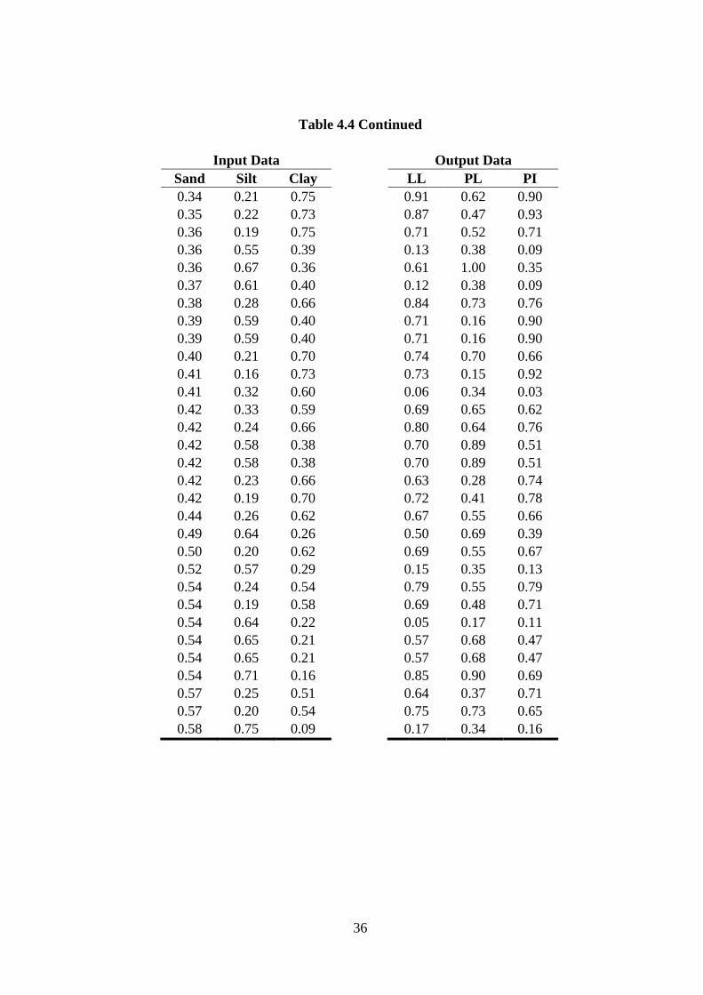
Table 4.4 Continued
Input Data Output Data Sand Silt Clay LL PL PI 0.34 0.21 0.75 0.91 0.62 0.90 0.35 0.22 0.73 0.87 0.47 0.93 0.36 0.19 0.75 0.71 0.52 0.71 0.36 0.55 0.39 0.13 0.38 0.09 0.36 0.67 0.36 0.61 1.00 0.35 0.37 0.61 0.40 0.12 0.38 0.09 0.38 0.28 0.66 0.84 0.73 0.76 0.39 0.59 0.40 0.71 0.16 0.90 0.39 0.59 0.40 0.71 0.16 0.90 0.40 0.21 0.70 0.74 0.70 0.66 0.41 0.16 0.73 0.73 0.15 0.92 0.41 0.32 0.60 0.06 0.34 0.03 0.42 0.33 0.59 0.69 0.65 0.62 0.42 0.24 0.66 0.80 0.64 0.76 0.42 0.58 0.38 0.70 0.89 0.51 0.42 0.58 0.38 0.70 0.89 0.51 0.42 0.23 0.66 0.63 0.28 0.74 0.42 0.19 0.70 0.72 0.41 0.78 0.44 0.26 0.62 0.67 0.55 0.66 0.49 0.64 0.26 0.50 0.69 0.39 0.50 0.20 0.62 0.69 0.55 0.67 0.52 0.57 0.29 0.15 0.35 0.13 0.54 0.24 0.54 0.79 0.55 0.79 0.54 0.19 0.58 0.69 0.48 0.71 0.54 0.64 0.22 0.05 0.17 0.11 0.54 0.65 0.21 0.57 0.68 0.47 0.54 0.65 0.21 0.57 0.68 0.47 0.54 0.71 0.16 0.85 0.90 0.69 0.57 0.25 0.51 0.64 0.37 0.71 0.57 0.20 0.54 0.75 0.73 0.65 0.58 0.75 0.09 0.17 0.34 0.16
Page 52
37
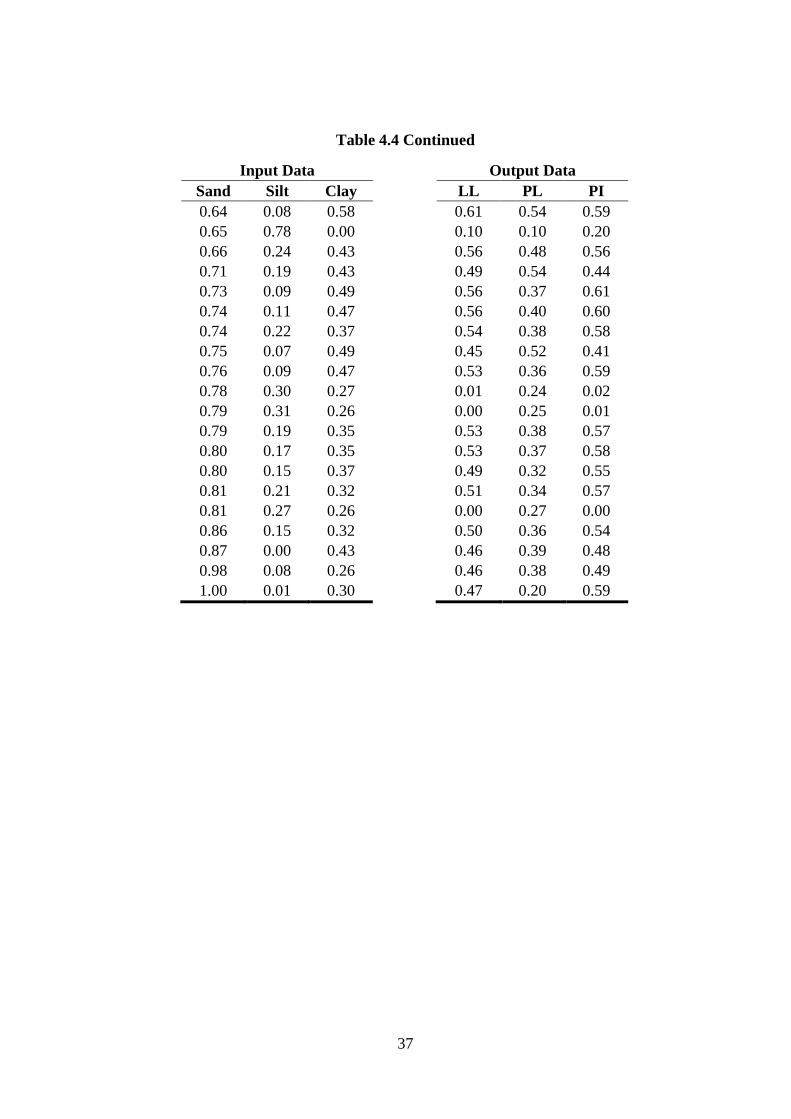
Table 4.4 Continued
Input Data Output Data Sand Silt Clay LL PL PI 0.64 0.08 0.58 0.61 0.54 0.59 0.65 0.78 0.00 0.10 0.10 0.20 0.66 0.24 0.43 0.56 0.48 0.56 0.71 0.19 0.43 0.49 0.54 0.44 0.73 0.09 0.49 0.56 0.37 0.61 0.74 0.11 0.47 0.56 0.40 0.60 0.74 0.22 0.37 0.54 0.38 0.58 0.75 0.07 0.49 0.45 0.52 0.41 0.76 0.09 0.47 0.53 0.36 0.59 0.78 0.30 0.27 0.01 0.24 0.02 0.79 0.31 0.26 0.00 0.25 0.01 0.79 0.19 0.35 0.53 0.38 0.57 0.80 0.17 0.35 0.53 0.37 0.58 0.80 0.15 0.37 0.49 0.32 0.55 0.81 0.21 0.32 0.51 0.34 0.57 0.81 0.27 0.26 0.00 0.27 0.00 0.86 0.15 0.32 0.50 0.36 0.54 0.87 0.00 0.43 0.46 0.39 0.48 0.98 0.08 0.26 0.46 0.38 0.49 1.00 0.01 0.30 0.47 0.20 0.59
Page 53
38
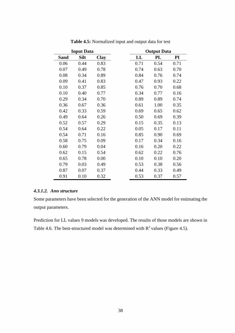
Table 4.5: Normalized input and output data for test
4.3.1.2. Ann structure
Some parameters have been selected for the generation of the ANN model for estimating the
output parameters.
Prediction for LL values 9 models was developed. The results of those models are shown in
Table 4.6. The best-structured model was determined with R2 values (Figure 4.5).
Input Data Output Data Sand Silt Clay LL PL PI 0.06 0.44 0.83 0.71 0.54 0.71 0.07 0.49 0.78 0.74 0.63 0.70 0.08 0.34 0.89 0.84 0.76 0.74 0.09 0.41 0.83 0.47 0.93 0.22 0.10 0.37 0.85 0.76 0.70 0.68 0.10 0.40 0.77 0.34 0.77 0.16 0.29 0.34 0.70 0.89 0.89 0.74 0.36 0.67 0.36 0.61 1.00 0.35 0.42 0.33 0.59 0.69 0.65 0.62 0.49 0.64 0.26 0.50 0.69 0.39 0.52 0.57 0.29 0.15 0.35 0.13 0.54 0.64 0.22 0.05 0.17 0.11 0.54 0.71 0.16 0.85 0.90 0.69 0.58 0.75 0.09 0.17 0.34 0.16 0.60 0.79 0.04 0.16 0.20 0.22 0.62 0.15 0.54 0.62 0.22 0.76 0.65 0.78 0.00 0.10 0.10 0.20 0.79 0.03 0.49 0.53 0.38 0.56 0.87 0.07 0.37 0.44 0.33 0.49 0.91 0.10 0.32 0.53 0.37 0.57
Page 54
39
Table 4.6: ANN models for LL prediction
R2
Model No Output
Number of
Layers
Number of
Neurons
Transfer Functions Training Validation Testing Adjust
R2
1 LL 2 5 Tansig Tansig 0.79 0.59 0.73 0.76
2 LL 2 5 Tansig Logsig 0.73 0.41 0.43 0.65
3 LL 2 5 Logsig Logsig 0.61 0.55 0.52 0.58
4 LL 2 7 Tansig Tansig 0.74 0.89 0.65 0.76
5 LL 2 7 Tansig Logsig 0.67 0.59 0.51 0.64
6 LL 2 7 Logsig Logsig 0.74 0.83 0.89 0.76
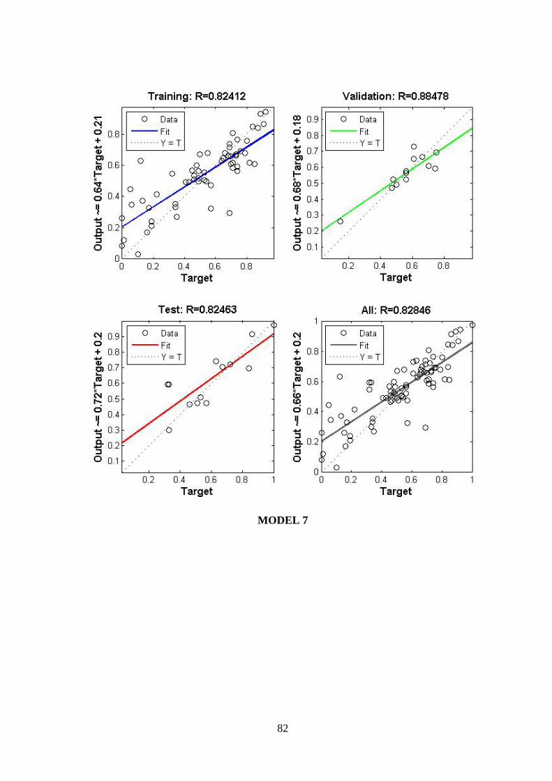
7 LL 2 10 Tansig Tansig 0.82 0.88 0.82 0.83
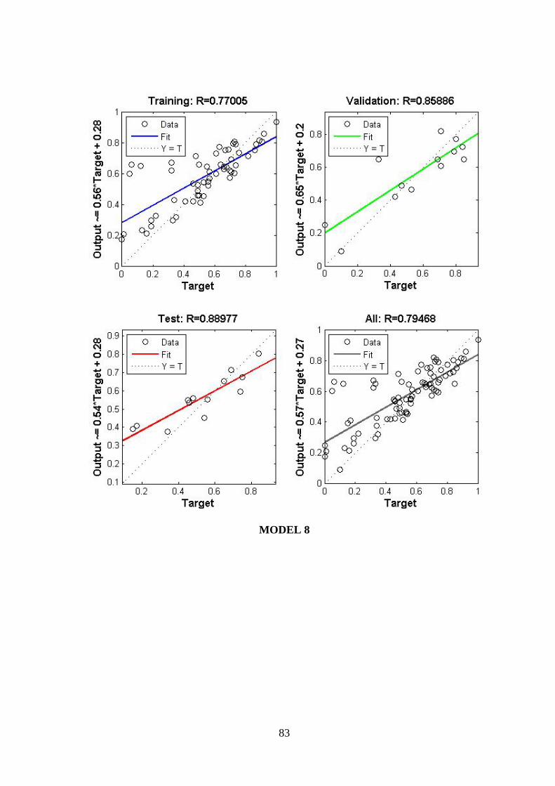
8 LL 2 10 Tansig Logsig 0.77 0.86 0.89 0.79
9 LL 2 10 Logsig Logsig 0.62 0.59 0.62 0.61
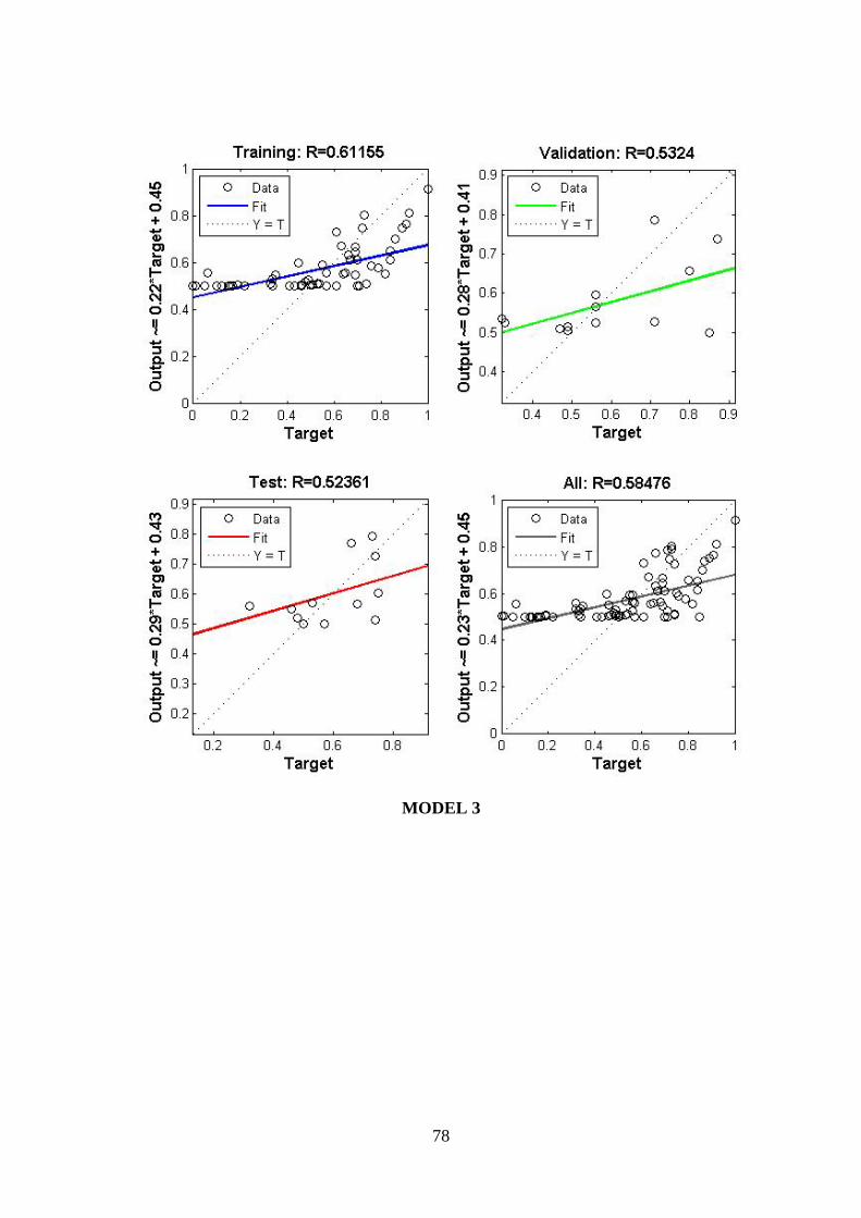
Regression analysis results of models are given in Appendix 2.
Figure 4.5: Comparison ANN models for predict LL
Page 55
40
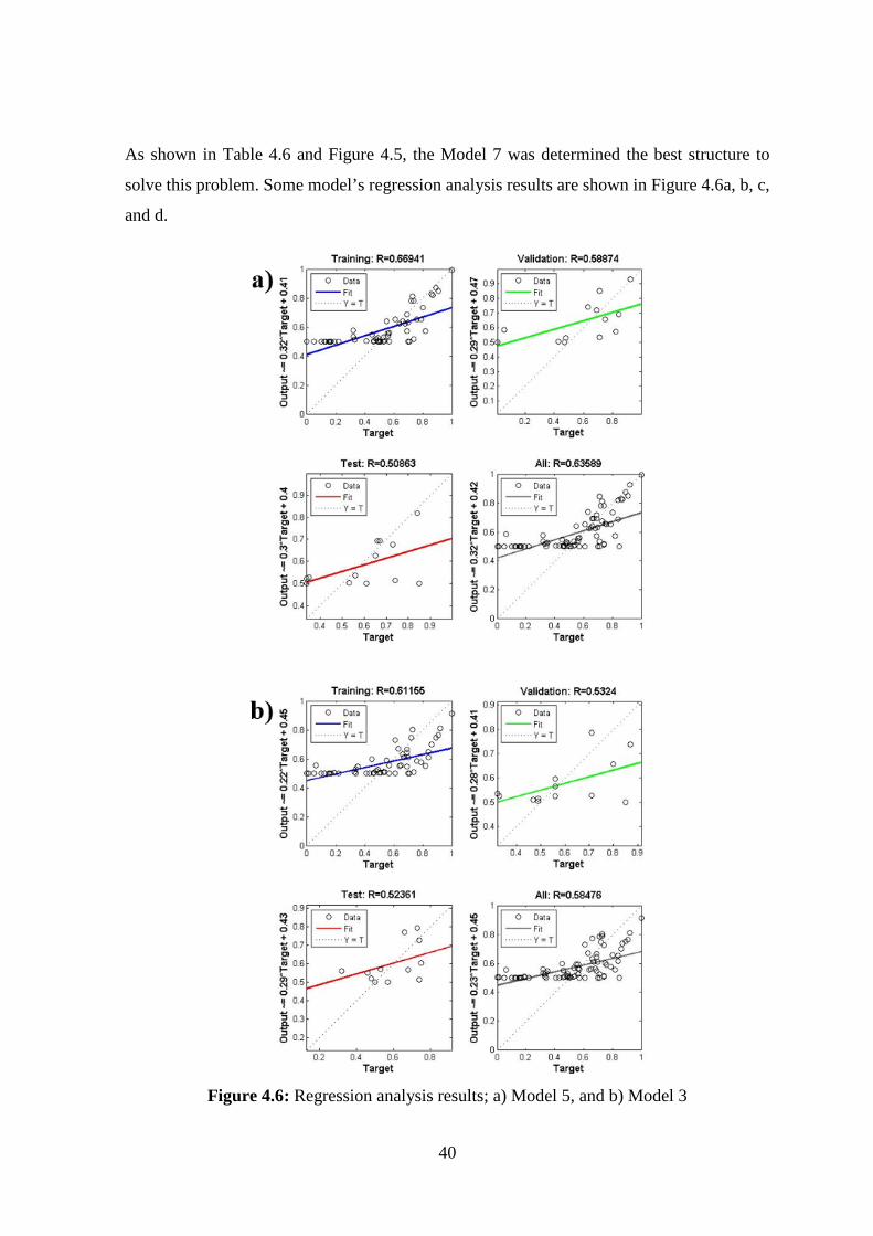
As shown in Table 4.6 and Figure 4.5, the Model 7 was determined the best structure to
solve this problem. Some model’s regression analysis results are shown in Figure 4.6a, b, c,
and d.
Figure 4.6: Regression analysis results; a) Model 5, and b) Model 3
Page 56
41
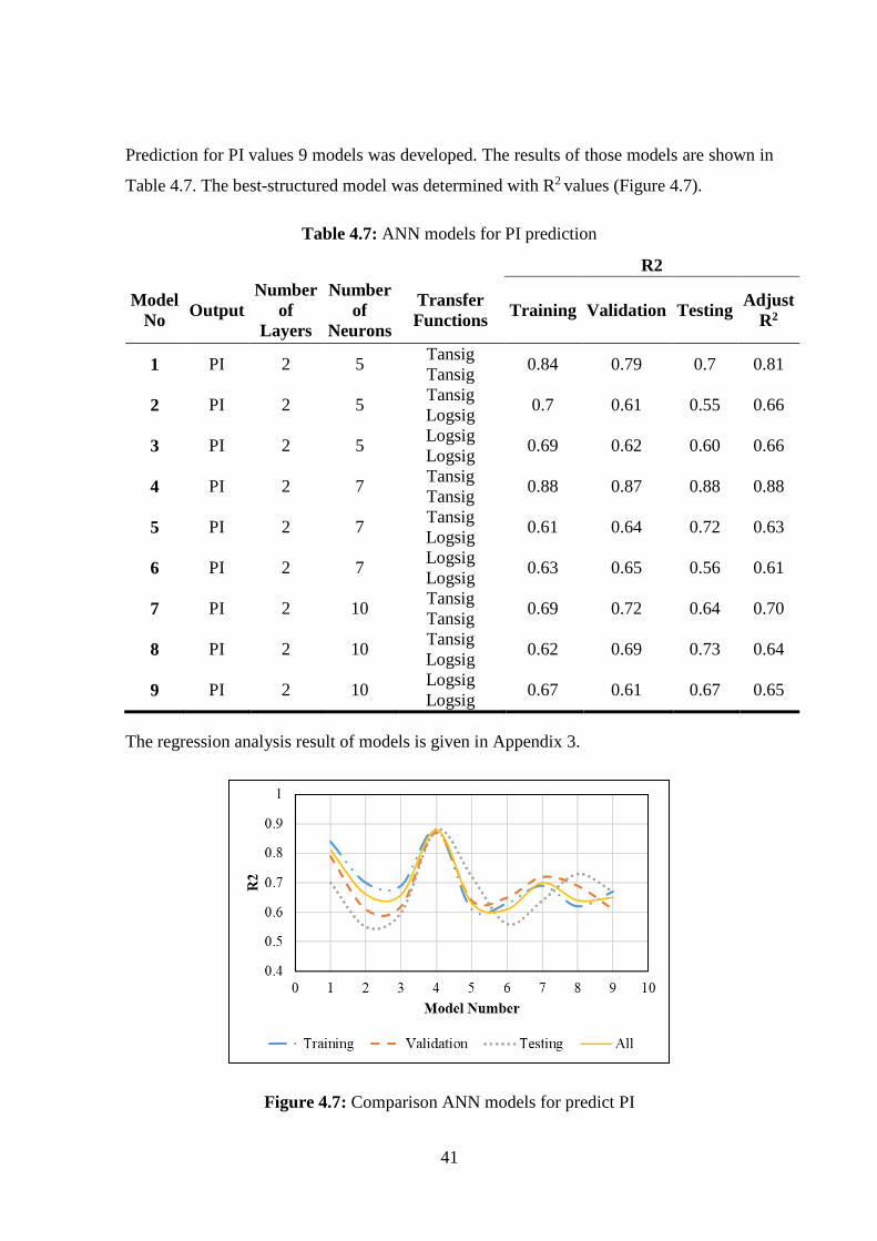
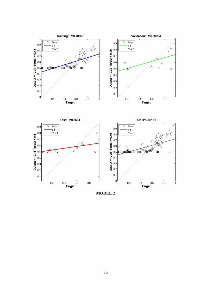
Prediction for PI values 9 models was developed. The results of those models are shown in
Table 4.7. The best-structured model was determined with R2 values (Figure 4.7).
Table 4.7: ANN models for PI prediction
R2
Model No Output
Number of
Layers
Number of
Neurons
Transfer Functions Training Validation Testing Adjust
R2
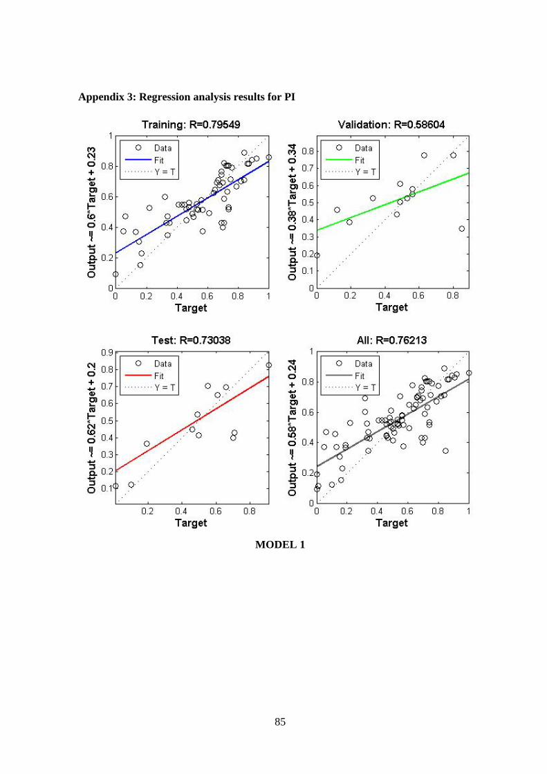
1 PI 2 5 Tansig Tansig 0.84 0.79 0.7 0.81
2 PI 2 5 Tansig Logsig 0.7 0.61 0.55 0.66
3 PI 2 5 Logsig Logsig 0.69 0.62 0.60 0.66
4 PI 2 7 Tansig Tansig 0.88 0.87 0.88 0.88
5 PI 2 7 Tansig Logsig 0.61 0.64 0.72 0.63
6 PI 2 7 Logsig Logsig 0.63 0.65 0.56 0.61
7 PI 2 10 Tansig Tansig 0.69 0.72 0.64 0.70
8 PI 2 10 Tansig Logsig 0.62 0.69 0.73 0.64
9 PI 2 10 Logsig Logsig 0.67 0.61 0.67 0.65
The regression analysis result of models is given in Appendix 3.
Figure 4.7: Comparison ANN models for predict PI
Page 57
42
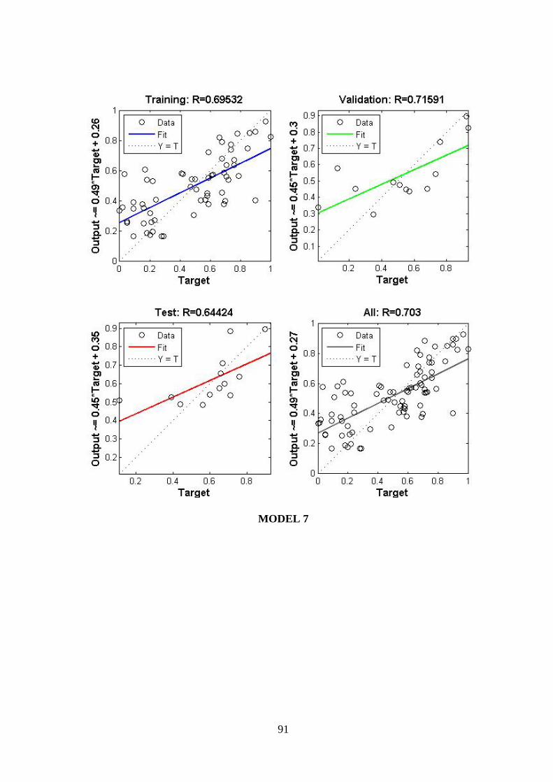
As shown in Table 4.7 and Figure 4.7, the Model 4 was determined the best structure to
solve this problem. Some model’s regression analysis results are shown in Figure 4.8a, b, c,
and d.
Figure 4.8: Regression analysis results; a) Model 2, and b) Model 7
Page 58
43
It has been tried to find optimum values while selecting these parameters that are given in
Table 4.8.
Backpropagation feedforward model was used in this study with supervised learning
technique. In the development of ANN tool, "nntool" tool which is available as a ready tool
in MatLab R2013a software is used. As a result of the models generated by selecting the
appropriate number of layers and hidden element values for each output parameter (Figure
4.9), the learning process is trained to achieve optimum results.
Table 4.8 ANN structure parameters
Parameters Values
LL PI
Input Parameter 3 3
Number of Layers 2 2
Number of Neurons 10 7
Transfer Function Tansig Tansig
Network Type Feed-forward backpropagation
Figure 4.9: ANN model sample
In figure 4.9 Input represents the grain size distribution data, w is weight, b is bias and Output
is LL or PI.
4.3.1.3. Ann training
Once the model is created, the system needs to be trained. The data for the training is written
in vector format according to the program. In the model 70% of the data were used for the
training, 15% for validation and 15% for the test.
Page 59
44
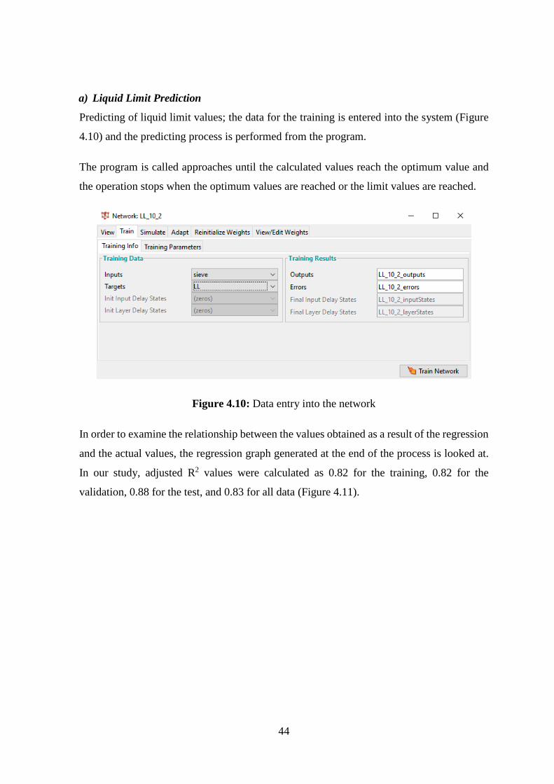
a) Liquid Limit Prediction
Predicting of liquid limit values; the data for the training is entered into the system (Figure
4.10) and the predicting process is performed from the program.
The program is called approaches until the calculated values reach the optimum value and
the operation stops when the optimum values are reached or the limit values are reached.
Figure 4.10: Data entry into the network
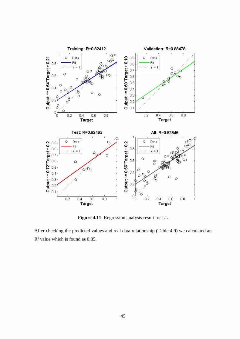
In order to examine the relationship between the values obtained as a result of the regression
and the actual values, the regression graph generated at the end of the process is looked at.
In our study, adjusted R2 values were calculated as 0.82 for the training, 0.82 for the
validation, 0.88 for the test, and 0.83 for all data (Figure 4.11).
Page 60
45
Figure 4.11: Regression analysis result for LL
After checking the predicted values and real data relationship (Table 4.9) we calculated an
R2 value which is found as 0.85.
Page 61
46
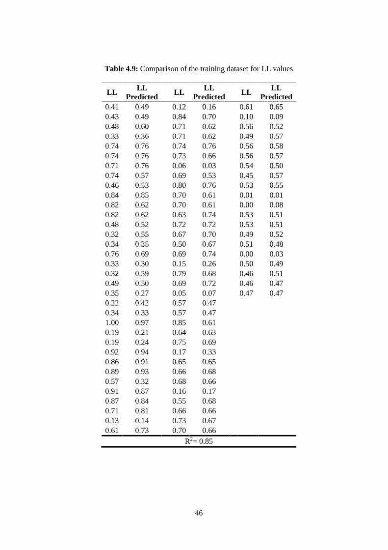
Table 4.9: Comparison of the training dataset for LL values
LL LL Predicted LL LL
Predicted LL LL Predicted
0.41 0.49 0.12 0.16 0.61 0.65 0.43 0.49 0.84 0.70 0.10 0.09 0.48 0.60 0.71 0.62 0.56 0.52 0.33 0.36 0.71 0.62 0.49 0.57 0.74 0.76 0.74 0.76 0.56 0.58 0.74 0.76 0.73 0.66 0.56 0.57 0.71 0.76 0.06 0.03 0.54 0.50 0.74 0.57 0.69 0.53 0.45 0.57 0.46 0.53 0.80 0.76 0.53 0.55 0.84 0.85 0.70 0.61 0.01 0.01 0.82 0.62 0.70 0.61 0.00 0.08 0.82 0.62 0.63 0.74 0.53 0.51 0.48 0.52 0.72 0.72 0.53 0.51 0.32 0.55 0.67 0.70 0.49 0.52 0.34 0.35 0.50 0.67 0.51 0.48 0.76 0.69 0.69 0.74 0.00 0.03 0.33 0.30 0.15 0.26 0.50 0.49 0.32 0.59 0.79 0.68 0.46 0.51 0.49 0.50 0.69 0.72 0.46 0.47 0.35 0.27 0.05 0.07 0.47 0.47 0.22 0.42 0.57 0.47 0.34 0.33 0.57 0.47 1.00 0.97 0.85 0.61 0.19 0.21 0.64 0.63 0.19 0.24 0.75 0.69 0.92 0.94 0.17 0.33 0.86 0.91 0.65 0.65 0.89 0.93 0.66 0.68 0.57 0.32 0.68 0.66 0.91 0.87 0.16 0.17 0.87 0.84 0.55 0.68 0.71 0.81 0.66 0.66 0.13 0.14 0.73 0.67 0.61 0.73 0.70 0.66
R2= 0.85
Page 62
47
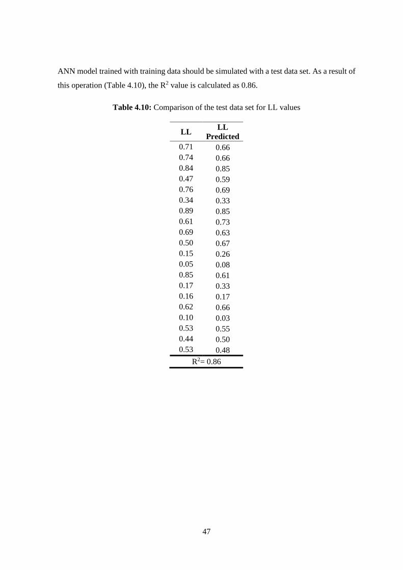
ANN model trained with training data should be simulated with a test data set. As a result of
this operation (Table 4.10), the R2 value is calculated as 0.86.
Table 4.10: Comparison of the test data set for LL values
LL LL Predicted
0.71 0.66 0.74 0.66 0.84 0.85 0.47 0.59 0.76 0.69 0.34 0.33 0.89 0.85 0.61 0.73 0.69 0.63 0.50 0.67 0.15 0.26 0.05 0.08 0.85 0.61 0.17 0.33 0.16 0.17 0.62 0.66 0.10 0.03 0.53 0.55 0.44 0.50 0.53 0.48
R2= 0.86
Page 63
48
The relationship with the real and predicted data of LL values is shown in Figure 4.12.
Figure 4.12: Comparison between real and predict data for LL
b) Plasticity Index Prediction
Predicting of plasticity index values; the data for the training is entered into the system
(Figure 4.13) and the predicting process is performed from the program.
The program operates until the calculated values reach the optimum values and it stops the
operation once the desired values are predicted (optimum values); in other words, the
program stops once the plasticity index values are predicted favorably.
0
10
20
30
40
50
60
70
80
90
100
1 12 23 34 45 56 67 78 89 100
LL
Sample Number
LL Results
Real Value Predict Value
Training Test
Page 64
49
Figure 4.13: Data entry into the network
In order to examine the relationship between the actual values and the predictions, the
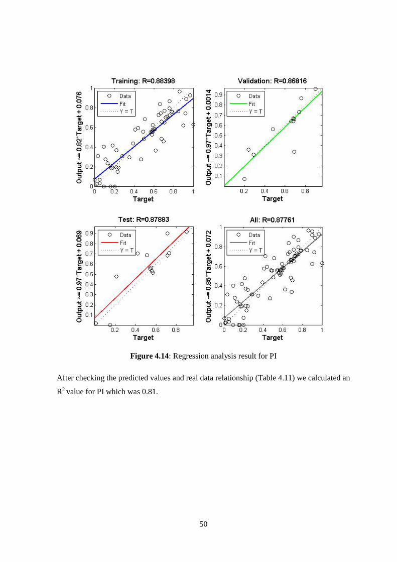
regression graph is plotted at the end of the training process. In our study, adjusted R2 for PI
values were calculated as 0.86 for the training, 0.87 for the validation, 0.88 for the test, and
0.87 for all data (Figure 4.14).
Page 65
50
Figure 4.14: Regression analysis result for PI
After checking the predicted values and real data relationship (Table 4.11) we calculated an
R2 value for PI which was 0.81.
Page 66
51
Table 4.11: Comparison of training data set for PI values
PI PI Predicted PI PI
Predicted PI PI Predicted
0.28 0.31 0.09 0.40 0.59 0.63 0.29 0.31 0.76 0.72 0.20 0.07 0.22 0.37 0.90 0.62 0.56 0.53 0.24 0.24 0.90 0.62 0.44 0.60 0.68 0.68 0.66 0.84 0.61 0.58 0.68 0.68 0.92 0.74 0.60 0.58 0.71 0.65 0.03 0.03 0.58 0.53 0.70 0.46 0.62 0.36 0.41 0.58 0.21 0.25 0.76 0.79 0.59 0.58 0.74 0.71 0.51 0.49 0.02 0.03 0.76 0.87 0.51 0.49 0.01 0.02 0.76 0.87 0.74 0.73 0.57 0.55 0.24 0.19 0.78 0.76 0.58 0.56 0.18 0.42 0.66 0.64 0.55 0.57 0.15 0.00 0.39 0.44 0.57 0.51 0.68 0.48 0.67 0.74 0.00 0.07 0.20 0.00 0.13 0.24 0.54 0.56 0.17 0.19 0.79 0.76 0.48 0.56 0.23 0.15 0.71 0.77 0.49 0.56 0.16 0.00 0.11 0.28 0.59 0.56 0.09 0.00 0.47 0.27 0.18 0.19 0.47 0.27 0.97 0.93 0.69 0.34 0.05 0.03 0.71 0.68 0.05 0.07 0.65 0.73 0.90 0.96 0.16 0.21 0.85 0.79 0.72 0.70 0.86 0.96 0.68 0.67 0.50 0.49 0.73 0.71 0.90 0.92 0.22 0.20 0.93 0.89 0.42 0.71 0.71 0.90 0.68 0.66 0.09 0.00 1.00 0.63 0.35 0.30 0.69 0.66
R2= 0.81
Page 67
52
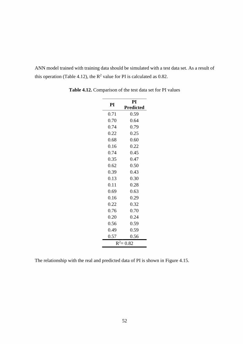
ANN model trained with training data should be simulated with a test data set. As a result of
this operation (Table 4.12), the R2 value for PI is calculated as 0.82.
Table 4.12. Comparison of the test data set for PI values
PI PI Predicted
0.71 0.59 0.70 0.64 0.74 0.79 0.22 0.25 0.68 0.60 0.16 0.22 0.74 0.45 0.35 0.47 0.62 0.50 0.39 0.43 0.13 0.30 0.11 0.28 0.69 0.63 0.16 0.29 0.22 0.32 0.76 0.70 0.20 0.24 0.56 0.59 0.49 0.59 0.57 0.56
R2= 0.82
The relationship with the real and predicted data of PI is shown in Figure 4.15.
Page 68
53
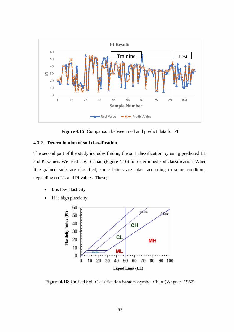
Figure 4.15: Comparison between real and predict data for PI
4.3.2. Determination of soil classification
The second part of the study includes finding the soil classification by using predicted LL
and PI values. We used USCS Chart (Figure 4.16) for determined soil classification. When
fine-grained soils are classified, some letters are taken according to some conditions
depending on LL and PI values. These;
• L is low plasticity
• H is high plasticity
Figure 4.16: Unified Soil Classification System Symbol Chart (Wagner, 1957)
0
10
20
30
40
50
60
1 12 23 34 45 56 67 78 89 100
PI
Sample Number
PI Results
Real Value Predict Value
Training Test
Page 69
54
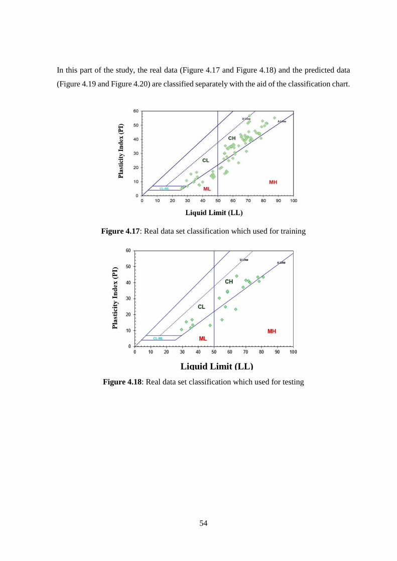
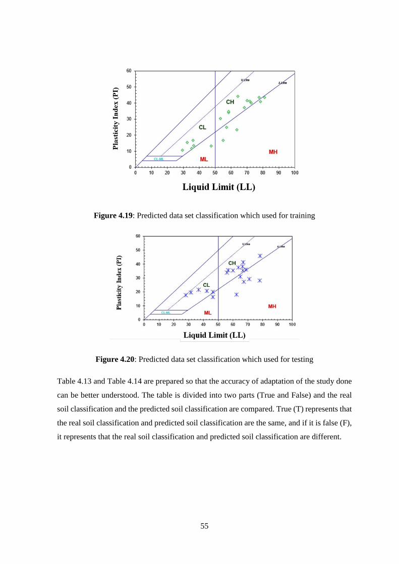
In this part of the study, the real data (Figure 4.17 and Figure 4.18) and the predicted data
(Figure 4.19 and Figure 4.20) are classified separately with the aid of the classification chart.
Figure 4.17: Real data set classification which used for training
Figure 4.18: Real data set classification which used for testing
Liquid Limit (LL)
Page 70
55
Figure 4.19: Predicted data set classification which used for training
Figure 4.20: Predicted data set classification which used for testing
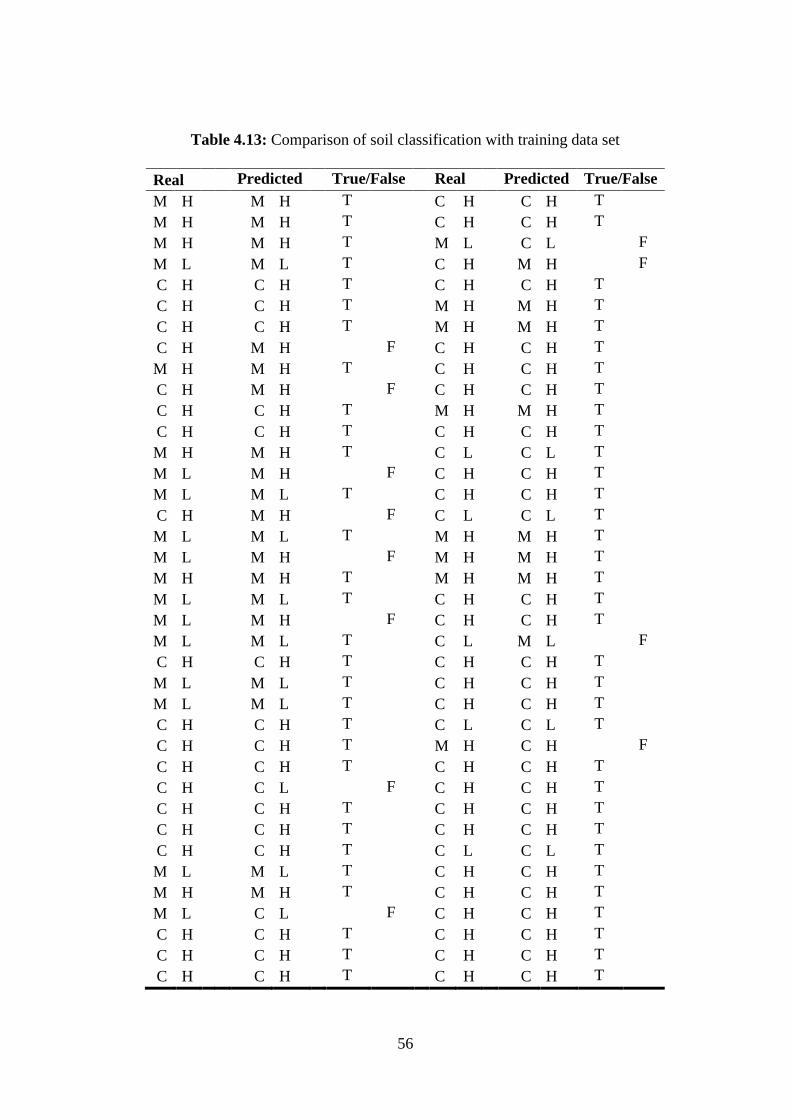
Table 4.13 and Table 4.14 are prepared so that the accuracy of adaptation of the study done
can be better understood. The table is divided into two parts (True and False) and the real
soil classification and the predicted soil classification are compared. True (T) represents that
the real soil classification and predicted soil classification are the same, and if it is false (F),
it represents that the real soil classification and predicted soil classification are different.
Page 71
56
Table 4.13: Comparison of soil classification with training data set
Real Predicted True/False Real Predicted True/False M H M H T C H C H T M H M H T C H C H T M H M H T M L C L F M L M L T C H M H F C H C H T C H C H T C H C H T M H M H T C H C H T M H M H T C H M H F C H C H T M H M H T C H C H T C H M H F C H C H T C H C H T M H M H T C H C H T C H C H T M H M H T C L C L T M L M H F C H C H T M L M L T C H C H T C H M H F C L C L T M L M L T M H M H T M L M H F M H M H T M H M H T M H M H T M L M L T C H C H T M L M H F C H C H T M L M L T C L M L F C H C H T C H C H T M L M L T C H C H T M L M L T C H C H T C H C H T C L C L T C H C H T M H C H F C H C H T C H C H T C H C L F C H C H T C H C H T C H C H T C H C H T C H C H T C H C H T C L C L T M L M L T C H C H T M H M H T C H C H T M L C L F C H C H T C H C H T C H C H T C H C H T C H C H T C H C H T C H C H T
Page 72
57
Table 4.13 Continued
Real Predicted True/False C H C H T C L C L T C L M L F C H C H T C H C H T C H C H T C H C H T C L C L T C H C H T C H C H T C H C H T C H C H T 75 True/13 False = %85.22 Accuracy
As a result of the data used for training, 75 of the 88 classifications were found to be correct
in the soil classifications. This gives an accuracy of about 85%.
Table 4.14: Comparison of soil classification with test data set
Real Predicted True/False C H C H T C H C H T C H C H T M H M H T C H C H T M L M L T M H M H T M H M H T C H M H F M H M H T C L C L T C L C L T M H C H F C L C L T C L C L T C H C H T
Page 73
58
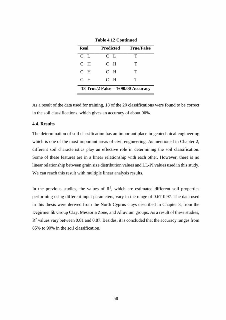
Table 4.12 Continued
Real Predicted True/False
C L C L T
C H C H T
C H C H T
C H C H T
18 True/2 False = %90.00 Accuracy
As a result of the data used for training, 18 of the 20 classifications were found to be correct
in the soil classifications, which gives an accuracy of about 90%.
4.4. Results
The determination of soil classification has an important place in geotechnical engineering
which is one of the most important areas of civil engineering. As mentioned in Chapter 2,
different soil characteristics play an effective role in determining the soil classification.
Some of these features are in a linear relationship with each other. However, there is no
linear relationship between grain size distribution values and LL-PI values used in this study.
We can reach this result with multiple linear analysis results.
In the previous studies, the values of R2, which are estimated different soil properties
performing using different input parameters, vary in the range of 0.67-0.97. The data used
in this thesis were derived from the North Cyprus clays described in Chapter 3, from the
Değirmenlik Group Clay, Mesaoria Zone, and Alluvium groups. As a result of these studies,
R2 values vary between 0.81 and 0.87. Besides, it is concluded that the accuracy ranges from
85% to 90% in the soil classification.
Page 74
59
CHAPTER 5
CONCLUSIONS AND RECOMMENDATIONS
5.1. Conclusions
ANN, which is becoming more widespread in the fields of science and engineering, is also
a useful method in geotechnical engineering fields. This study presents the advantages of
using ANN in cases where classical regression methods are inadequate. In total, 108 data
sets are used in the development of the ANN tool. It was aimed to maximize the validity of
the program with selected examples from North Cyprus.
The following conclusions can be reached as a result of the studies carried out;
1. There is no direct relationship between the liquid limit and plasticity index and sieve
analysis values.
2. The tansig transfer function among the transfer functions for the data used in this
study enabled us to achieve better results than the logsig transfer function.
3. As a result of the study with ANN, a connection could be made between the
parameters that are not directly related.
4. By using the ANN method, we can reach the sieve analysis values and the Atterberg
values with a high accuracy rate.
5. There is a higher connection between the LL values and the sieve analysis values
than PI values.
6. The validity and accuracy of the system have been tested by making the soil
classification with the LL and PI values as a result of the ANN.
7. ANN can successfully apply in engineering problems that are more affected by
variables such as soil properties.
8. No attempt was made to find the relationship of different soils.
Page 75
60
5.2. Recommendations
1. This study was carried out only on North Cyprus soils, especially on the clays. Work
areas and parameters can be expanded during future work.
2. Similar work within the same soil groups will point out the relationship of the soils
with different swelling potential
Page 76
61
REFERENCES
Abu-Kiefa, M. A. (1998). General regression neural networks for driven piles in
cohesionless soils. Journal of Geotechnical and Geoenvironmental Engineering,
124(12), 1177–1185.
Afram, A., Janabi-Sharifi, F., Fung, A. S. & Raahemifar, K. (2017). Artificial neural network
(ANN) based model predictive control (MPC) and optimization of HVAC systems: A
state of the art review and case study of a residential HVAC system. Energy and
Buildings, 141, 96–113. https://doi.org/10.1016/J.ENBUILD.2017.02.012
Ahmad, I., El Naggar, M. H. & Khan, A. N. (2007). Artificial neural network application to
estimate kinematic soil pile interaction response parameters. Soil Dynamics and
Earthquake Engineering, 27(9), 892–905.
Akkaya, G. (2011). Artificial Neural Networks and Their Applications In Agriculture.
Journal of the Faculty of Agriculture; Cilt 38, Sayı 2 (2007), 14-30.
Archer, J. R. (1975). Soil consistency. Soil Physical Conditions and Crop Production. Tech.
Bull, (29), 289–297.
Aslantaş, V. & Kurban, R. (2007). Artificial neural networks and applications in
geographical information systems. In TMMOB Harita ve Kadastro Mühendisleri Odası
Ulusal Coğrafi Bilgi Sistemleri Kongresi. Trabzon.
Aslay, F. & Üstün, Ö. (2013). Estimating Soil Temperature With Artificial Neural Networks
Using Meteorological Parameters. Politeknik Dergisi, 16(4), 139-145.
ASTM D422-63(2007)e2, Standard Test Method for Particle-Size Analysis of Soils
(Withdrawn 2016), ASTM International, West Conshohocken, PA, 2007,
www.astm.org
ASTM D4318-17e1, Standard Test Methods for Liquid Limit, Plastic Limit, and Plasticity
Index of Soils, ASTM International, West Conshohocken, PA, 2017, www.astm.org
ASTM D6913 / D6913M-17, Standard Test Methods for Particle-Size Distribution
Page 77
62
(Gradation) of Soils Using Sieve Analysis, ASTM International, West Conshohocken,
PA, 2017, www.astm.org
Atalar, C. (2002). Swelling Clays: A continuous threat to the built environment of
Cyprus .Report of Turkish Cypriot Chamber of MMG Engineers,(contributed by
Tandoğdu, Y., Acar, A., Bilsel, H. & Necdet, M.), Lefkoşa, TRNC.
Atalar, C. (2004). Foundation design for swelling clays of north Nicosia. In Proceedings of
the International Conference on Geotechnical Engineering, Sharjah, UAE (pp. 121–
128).
Atalar, C. (2005). The origin and characteristics of Cyprus clays. In Extended Abstract Book
of 57th Geological Congress of Turkey, Ankara (pp. 144–148).
Atalar, C. (2006). Engineering Properties and Problems of Cyprus Soils. In Proceedings of
the Symposium on Recent Applications in Engineering Geology, 25-27 May 2006
Denizli, Turkey (pp. 629–638).
Atalar, C. & Das, B. M. (2009). Geotechnical properties of Nicosia soils, Cyprus. In Proc.,
2th Int. Con. On New Developments in Soil Mechanics and Geotechnical Engineering
(pp. 360–367).
Atalar, C. & Das, B. M. (2018). Recent landslides in North Cyprus. Ce/Papers, 2(2–3), 409–
414. https://doi.org/10.1002/cepa.705
Atterberg, A. (1911). Plastizität des Bariumsulfats. Zeitschrift Für Angewandte Chemie,
24(49), 2355–2355. https://doi.org/10.1002/ange.19110244906
Bahmed, I. T., Harichane, K., Ghrici, M., Rebouh, R., & Gadouri, H. (2017). Prediction of
geotechnical properties of clayey soils stabilised with lime using artificial neural
networks (ANNs). International Journal of Geotechnical Engineering.
https://doi.org/10.1080/19386362.2017.1329966
Basma, A. A. & Kallas, N. (2004). Modeling soil collapse by artificial neural networks.
Geotechnical & Geological Engineering, 22(3), 427–438.
Page 78
63
https://doi.org/10.1023/B:GEGE.0000025044.72718.db
Brain Education. (2018). Retrieved December 4, 2018, from
https://www.morphonix.com/braineducation/
Cal, Y. (1995). Soil classification by neural network. Advances in Engineering Software,
22(2), 95–97.
Campbell, D. (2001). Liquid and plastic limits. In K. Smith & C. Mullins (Eds.), Soil and
Environmental Analysis, Physical Methods (pp. 349–375). New York: Dekker Inc.
Casagrande, A. (1958). Notes on the Design of the Liquid Limit Device. In Géotechnique
(pp. 84–91).
Chan, W. T., Chow, Y. K. & Liu, L. F. (1995). Neural network: an alternative to pile driving
formulas. Computers and Geotechnics, 17(2), 135–156.
Chin, W. W. (1998). The partial least squares approach to structural equation modeling.
Modern Methods for Business Research, 295(2), 295–336.
Das, B. M. (2010). Principles of Geotechnical Engineering (Seventh Ed). Stamford, CT:
CENGAGE Learning.
Das, S. K. & Basudhar, P. K. (2006). Undrained lateral load capacity of piles in clay using
artificial neural network. Computers and Geotechnics, 33(8), 454–459.
De la Rosa, D. (1979). Relation of several pedological characteristics to engineering qualities
of soil. Journal of Soil Science, 30(4), 793–799.
Dindar, H., Dimililer, K., Özdağ, Ö. C., Atalar, C., Akgün, M. & Özyankı, A. (2017).
Vulnerability Index Assessment Using Neural Networks (Viann): A Case Study Of
Nicosia, Cyprus. ISPRS Annals of Photogrammetry, Remote Sensing & Spatial
Information Sciences, 4.
Elmas, Ç. (2007). Yapay zeka uygulamaları [Artificial intelligence applications]. Seçkin
Yayıncılık, Ankara.
Page 79
64
Garip, Z. Ş. (2011). Yapay sinir ağları ile mevcut yapıların deprem diski açısından durum
tespiti [Situation detection of current structures with artificial neural networks in terms
of earthquake risk]. Doktora Tezi. Sakarya Üniversitesi.
Geological Survey Department (GSD). (2002). Geotechnical map of Nicosia. Scale
1:25,000. Edited by G. Constantinou (Director) Nicosia, Cyprus.
Geotest. (2014). Adelya Rezidance Project.
Ghaleini, E. N., Koopialipoor, M., Momenzadeh, M., Sarafraz, M. E., Mohamad, E. T. &
Gordan, B. (2018). A combination of artificial bee colony and neural network for
approximating the safety factor of retaining walls. Engineering with Computers, 0(0),
1–12. https://doi.org/10.1007/s00366-018-0625-3
Goh, A. T. C. (1994). Nonlinear modelling in geotechnical engineering using neural
networks. Transactions of the Institution of Engineers, Australia. Civil Engineering,
36(4), 293–297.
Goh, A. T. C. (1996). Pile driving records reanalyzed using neural networks. Journal of
Geotechnical Engineering, 122(6), 492–495.
Goh, A. T. C., Kulhawy, F. H. & Chua, C. G. (2005). Bayesian neural network analysis of
undrained side resistance of drilled shafts. Journal of Geotechnical and
Geoenvironmental Engineering, 131(1), 84–93.
Goh, A. T. C., Wong, K. S. & Broms, B. B. (1995). Estimation of lateral wall movements in
braced excavations using neural networks. Canadian Geotechnical Journal, 32(6),
1059–1064.
Günaydın, O. (2009). Estimation of soil compaction parameters by using statistical analyses
and artificial neural networks. Environmental Geology, 57(1), 203–215.
https://doi.org/10.1007/s00254-008-1300-6
Hamzaçebi, C. (2011). Yapay sinir ağları: tahmin amaçlı kullanımı MATLAB ve
Neurosolutions uygulamalı [Artificial neural networks: predictive use of MATLAB and
Page 80
65
Neurosolutions applied]. Ekin Basım Yayın Dağıtım.
Hanna, A. M., Morcous, G. & Helmy, M. (2004). Efficiency of pile groups installed in
cohesionless soil using artificial neural networks. Canadian Geotechnical Journal,
41(6), 1241–1249.
Hassannejad, H., Sirus, M. & Mehdizadeh, R. (2015). Comparison and Evaluation of
Artificial Neural Network ( ANN ) Training Algorithms in Predicting Soil Type
Classification. Bulletin of Environment, Pharmacology and Life Sciences, 4(1), 212–
218. Retrieved from http://www.bepls.com
Haykin, S. & Network, N. (2004). A comprehensive foundation. Neural Networks, 2(2004),
41.
Hinton, G. E., Sejnowski, T. J., & Poggio, T. A. (1999). Unsupervised learning: foundations
of neural computation. MIT press.
Holtz, R. D., Kovacs, W. D. & Sheahan, T. C. (2011). An introduction to geotechnical
engineering (2nd ed.). Upper Saddle River (NJ): Pearson.
Hurtado, J. E., Londoño, J. M. & Meza, M. A. (2001). On the applicability of Neural
Networks for soil dynamic amplification analysis. Soil Dynamics and Earthquake
Engineering, 21(7), 579–591. https://doi.org/10.1016/S0267-7261(01)00037-9
Hussain, A. H. A. (2016). Prediction of compaction characteristics of over-consolidated
soils. Near East University.
Johnson, J., Li, J., & Chen, Z. (2000). Reinforcement Learning: An Introduction: R.S. Sutton,
A.G. Barto, MIT Press, Cambridge, MA 1998, 322 pp. ISBN 0-262-19398-1.
Neurocomputing (Vol. 35).
Jong, E. D., Acton, D. F. & Stonehouse, H. B. (1990). Estimating the Atterberg limits of
southern Saskatchewan soils from texture and carbon contents. Canadian Journal of
Soil Science, 70(4), 543–554.
Kakıcı, A. (2017). Yapay Sinir Ağları Mimarisi ve Yapı Elemanları #2 [Artificial Neural
Page 81
66
Networks Architecture and Structure Elements # 2]. Retrieved August 25, 2017, from
https://yapayzeka.ai/yapay-sinir-aglarinin-mimarisi-ve-yapi-elemanlari-2/
Kanungo, D. P., Sharma, S. & Pain, A. (2014). Artificial Neural Network (ANN) and
Regression Tree (CART) applications for the indirect estimation of unsaturated soil
shear strength parameters. Frontiers of Earth Science, 8(3), 439–456.
Kaynar, O., Görmez, Y., IŞIK, Y. E., & Demirkoparan, F. (2016). Değişik Kümeleme
Algoritmalarıyla Eğitilmiş Radyal Tabanlı Yapay Sinir Ağlarıyla Saldırı Tespiti
[Intrusion Detection with Radial Basis Neural Network Trained with Different
Clustering Algorithm]. In International Artificial Intelligence and Data Processing
Symposium (IDAP’16). Malatya/Turkey.
Keller, T. & Dexter, A. R. (2012). Plastic limits of agricultural soils as functions of soil
texture and organic matter content. Soil Research, 50(1), 7–17.
Ketin, İ. (1987). Ana hatlarıyla Kıbrıs’ın Jeolojisi ve Güney Anadolu ile Bağıntısı [Outlines
of the Geology of Cyprus and Its Comparison with the Southern Anatolia]. Bulletin of
Earth Sciences Application and Research Centre of Hacettepe University, 14, 207–229.
Kulga, B., Artun, E. & Ertekin, T. (2018). Characterization of tight-gas sand reservoirs from
horizontal-well performance data using an inverse neural network. Journal of Natural
Gas Science and Engineering, 59(May), 35–46.
https://doi.org/10.1016/j.jngse.2018.08.017
Lee, I. M. & Lee, J. H. (1996). Prediction of pile bearing capacity using artificial neural
networks. Computers and Geotechnics, 18(3), 189–200.
Lee, S. J., Lee, S. R. & Kim, Y. S. (2003). An approach to estimate unsaturated shear strength
using artificial neural network and hyperbolic formulation. Computers and
Geotechnics, 30(6), 489–503. https://doi.org/10.1016/S0266-352X(03)00058-2
Lippmann, R. (1987). An introduction to computing with neural nets. IEEE Assp Magazine,
4(2), 4–22.
Page 82
67
Mbagwu, J. S. C. & Abeh, O. G. (1998). Prediction of engineering properties of tropical
soils using intrinsic pedological parameters. Soil Science, 163(2), 93–102.
McBride, R. A. (2008). Soil consistency and lower plastic limit. In M. R. Carter & E. G.
Gregorich (Eds.), Soil Sampling and Methods of Analysis (2nd ed., pp. 761–769). CRC
Press.
Mikolov, T., Karafiát, M., Burget, L., Cernocký, J., & Khudanpur, S. (2010). Recurrent
neural network based language model. Proceedings of the 11th Annual Conference of
the International Speech Communication Association, INTERSPEECH 2010.
Miljkovic, D. (2010). Review of novelty detection methods. MIPRO, 2010 Proceedings of
the 33rd International Convention, (May 2010), 593–598.
https://doi.org/10.1242/jeb.02365
Najjar, Y. M., Basheer, I. A. & Naouss, W. A. (1996). On the identification of compaction
characteristics by neuronets. Computers and Geotechnics, 18(3), 167–187.
https://doi.org/https://doi.org/10.1016/0266-352X(95)00030-E
Nawari, N. O., Liang, R. & Nusairat, J. (1999). Artificial intelligence techniques for the
design and analysis of deep foundations. Electronic Journal of Geotechnical
Engineering, 4, 1–21.
Odell, R. T., Thornburn, T. H. & McKenzie, L. J. (1960). Relationships of Atterberg Limits
to Some Other Properties of Illinois Soils 1. Soil Science Society of America Journal,
24(4), 297–300.
Öztemel, E. (2003). Yapay Sinir Ağlari [Artificial Neural Network]. Papatya Yayincilik,
Istanbul.
Ozturk, T. E. (2014). Artificial neural networks approach for earthquake deformation
determination of geosynthetic reinforced retaining walls. International Journal of
Intelligent Systems and Applications in Engineering, 2(1), 1–9.
PCA. (1992). PCA Soil Primer. IL: Portland Cement Association: Skokie.
Page 83
68
Rafiq, M. Y., Bugmann, G. & Easterbrook, D. J. (2001). Neural network design for
engineering applications. Computers and Structures, 79(17), 1541–1552.
https://doi.org/10.1016/S0045-7949(01)00039-6
Rahman, M. S., Wang, J., Deng, W. & Carter, J. P. (2001). A neural network model for the
uplift capacity of suction caissons. Computers and Geotechnics, 28(4), 269–287.
Rankine, R. M. & Sivakugan, N. (2005). Prediction of paste backfill performance using
artificial neural networks.
Ranković, V., Novaković, A., Grujović, N., Divac, D. & Milivojević, N. (2014). Predicting
piezometric water level in dams via artificial neural networks. Neural Computing and
Applications, 24(5), 1115–1121.
Reale, C., Gavin, K., Libri, L., & Juri, D. (2018). Automatic classification of fine-grained
soils using CPT measurements and Artificial Neural Networks. Advanced Engineering
Informatics, 36, 207–215. https://doi.org/10.1016/j.aei.2018.04.003
Sağıroğlu, Ş., Beşdok, E. & Erler, M. (2003). Mühendislikte yapay zeka uygulamaları-1:
Yapay sinir ağları [Artificial intelligence applications in engineering-1: Artificial
neural networks]. Ufuk Kitap Kırtasiye-Yayıncılık.
Seybold, C. A., Engel, R. J. & Elrashidi, M. A. (2008). Linear regression models to estimate
soil liquid limit and plasticity index from basic soil properties. Soil Science, 173(1), 25–
34. https://doi.org/10.1097/ss.0b013e318159a5e1
Shahin, M. A. & Jaksa, M. B. (2006). Pullout capacity of small ground anchors by direct
cone penetration test methods and neural networks. Canadian Geotechnical Journal,
43(6), 626–637.
Shahin, M. A. & Jaksa, M. B. (2009). Intelligent computing for predicting axial capacity of
drilled shafts. In Contemporary Topics in In Situ Testing, Analysis, and Reliability of
Foundations (pp. 26–33).
Shahin, M. A., Jaksa, M. B. & Maier, H. R. (2004). Application of neural networks in
Page 84
69
foundation engineering. In Theme paper to the International e-Conference on Modern
Trends in Foundation Engineering: Geotechnical Challenges and Solutions, Theme.
Shahin, M. A., Jaksa, M. B. & Maier, H. R. (2005). Neural network based stochastic design
charts for settlement prediction. Canadian Geotechnical Journal, 42(1), 110–120.
Shang, J. Q., Ding, W., Rowe, R. K. & Josic, L. (2004). Detecting heavy metal contamination
in soil using complex permittivity and artificial neural networks. Canadian
Geotechnical Journal, 41(6), 1054–1067.
Sivakugan, N., Eckersley, J., & Li, H. (1998). Settlement predictions using neural networks. Australian Civil Engineering Transactions, 40, 49.
Stojanovic, B., Milivojevic, M., Milivojevic, N. & Antonijevic, D. (2016). A self-tuning
system for dam behavior modeling based on evolving artificial neural networks.
Advances in Engineering Software, 97, 85–95.
Taylor, D. (1948). Fundamentals of soil mechanics. Chapman And Hall, Limited.; New
York.
Teh, C. I., Wong, K. S., Goh, A. T. C. & Jaritngam, S. (1997). Prediction of pile capacity
using neural networks. Journal of Computing in Civil Engineering, 11(2), 129–138.
Tenpe, A. & Kaur, S. (2015). Artificial Neural Network Modeling for Predicting
Compaction Parameters based on Index Properties of Soil. International Journal of
Science and Research (IJSR), 4(7), 1198–1202.
Wagner, A. A. (1957). The use of the unified soil classification system by the bureau of
reclamation. In Proceedings of the 4th International Conference on Soil Mechanics and
Foundation Engineering, London (Vol. 1, p. 125).
Wroth, C. P. & Wood, D. M. (1978). The correlation of index properties with some basic
engineering properties of soils. Canadian Geotechnical Journal, 15(2), 137–145.
Yang, Y. & Zhang, Q. (1998). The application of neural networks to rock engineering
systems (RES). International Journal of Rock Mechanics and Mining Sciences, 35(6),
Page 85
70
727–745. https://doi.org/10.1016/S0148-9062(97)00339-2
Yingjie, Y. & Rosenbaum, M. S. (2002). The artificial neural network as a tool for assessing
geotechnical properties. Geotechnical & Geological Engineering, 20(2), 149–168.
Yuanyou, X., Yanming, X. & Ruigeng, Z. (1997). An engineering geology evaluation
method based on an artificial neural network and its application. Engineering Geology,
47(1–2), 149–156.
Page 87
72
Appendix 1: Samples used in this study
INPUTS
OUTPUTS
Sand Silt Clay LL PI
49.7 9.3 41.0 55.0 35.4 48.9 12.1 39.0 54.6 30.3 45.2 12.8 42.0 58.5 34.7 43.3 8.7 48.0 54.5 30.1 43.2 11.9 45.0 53.2 30.3 42.9 15.2 42.0 56.8 33.2 40.4 17.6 42.0 57.8 34.6 40.0 15.0 45.0 56.3 33.6 39.9 16.1 44.0 58.9 35.1 39.2 16.8 44.0 58.7 34.4 39.1 9.9 51.0 58.5 34.2 37.6 12.4 50.0 58.9 35.3 37.4 11.6 51.0 54.0 26.2 36.8 18.2 45.0 59.1 34.8 36.7 13.3 50.0 60.7 35.9 36.5 12.5 51.0 60.3 36.5 35.3 16.7 48.0 56.0 27.7 32.8 19.2 48.0 60.8 34.1 32.0 12.1 56.0 63.8 35.5 31.6 15.4 53.0 69.0 40.7 31.3 10.7 58.0 71.0 56.7 30.8 15.2 54.0 64.2 44.2 30.8 15.2 54.0 66.5 40.3 30.3 16.7 53.0 59.9 26.6 29.8 18.2 52.0 67.9 42.9 29.6 12.4 58.0 66.7 40.1 29.1 18.9 52.0 65.9 42.1 28.7 17.3 54.0 72.0 38.7 28.7 19.3 52.0 65.4 41.6 27.0 17.0 56.0 68.3 41.6
Page 88
73
INPUTS OUTPUTS Sand Silt Clay LL PI 22.2 19.9 58.0 67.5 38.9 21.2 16.8 62.0 70.4 45.4 21.2 18.8 60.0 65.0 43.4 21.1 19.0 60.0 75.5 44.5 20.4 15.6 64.0 71.0 52.7 20.2 17.8 62.0 71.4 38.9 19.2 20.8 60.0 77.6 44.3 18.2 16.8 65.0 69.5 41.7 17.7 18.3 64.0 79.5 53.0 17.3 17.7 65.0 81.8 51.5 16.5 23.5 60.0 61.2 30.8 15.5 18.5 66.0 80.9 49.6 14.9 20.1 65.0 78.9 48.9 14.8 23.2 62.0 81.0 43.5 14.7 17.3 68.0 82.7 51.3 7.6 14.4 78.0 87.5 55.2 40.4 20.4 39.2 26.3 5.1 39.1 21.9 39.0 26.5 5.6 38.9 21.8 39.3 26.8 6.2 32.6 42.1 25.3 32.3 15.4 30.2 42.5 27.3 36.1 16.7 29.1 41.1 29.8 36.6 13.5 27.2 39.1 33.7 78.5 40.9 27.1 36.1 36.8 29.5 10.8 27.1 36.7 36.2 61.4 29.6 26.2 33.3 40.5 35.3 11.8 24.6 36.3 39.1 57.2 25.0 21.1 33.5 45.4 68.9 31.5
Page 89
74
INPUTS OUTPUTS Sand Silt Clay LL PI 5.3 26.3 66.0 46.9 12.7 21.0 22.8 56.2 68.4 37.1 20.7 22.3 57.0 30.0 6.8 19.6 34.2 46.2 69.9 51.4 18.5 35.0 46.5 33.9 9.8 18.3 32.5 46.0 34.2 9.9 18.3 37.6 44.1 63.7 23.4 14.0 30.0 56.0 38.0 7.5 13.8 29.2 57.0 37.7 7.8 7.3 51.7 41.0 47.1 14.6 7.0 25.2 65.0 47.7 13.6 7.0 36.0 57.0 40.0 9.8 5.5 26.1 66.0 47.4 13.2 5.4 26.9 65.0 46.8 15.4 5.4 25.6 69.0 45.9 14.1 5.4 31.6 63.0 56.3 17.0 5.3 24.7 70.0 72.6 40.1 5.3 26.7 68.0 45.7 14.2 4.8 28.2 67.0 55.7 17.5 4.6 26.4 69.0 55.1 16.7 4.6 26.0 69.4 76.7 44.3 4.5 23.5 72.1 77.6 43.5 4.4 32.6 63.0 54.6 15.7 4.1 29.7 66.2 71.8 41.2 3.3 27.7 69.0 70.0 41.6 3.1 29.4 67.5 71.7 40.1 2.9 30.1 67.0 46.8 17.4 2.5 28.5 69.0 55.5 16.4 0.4 40.6 59.0 51.4 19.3 0.4 40.4 59.2 52.6 20.2
Page 90
75
INPUTS OUTPUTS
Sand Silt Clay LL PI
30.2 42.5 27.3 36.1 16.7
29.1 41.1 29.8 36.6 13.5
27.2 39.1 33.7 78.5 40.9
27.1 36.1 36.8 29.5 10.8
27.1 36.7 36.2 61.4 29.6
26.2 33.3 40.5 35.3 11.8
24.6 36.3 39.1 57.2 25.0
21.1 33.5 45.4 68.9 31.5
21.0 22.8 56.2 68.4 37.1
19.6 34.2 46.2 69.9 51.4
18.3 37.6 44.1 63.7 23.4
5.3 24.7 70.0 72.6 40.1
4.6 26.0 69.4 76.7 44.3
4.5 23.5 72.1 77.6 43.5
4.1 29.7 66.2 71.8 41.2
3.3 27.7 69.0 70.0 41.6
3.1 29.4 67.5 71.7 40.1
Page 91
76
Appendix 2: Regression analysis results for LL
MODEL 1
Page 100
85
Appendix 3: Regression analysis results for PI
MODEL 1
Page 109
THES
ISIN
BOX |
NO
W V
IEW
ING
: NEW
PAP
ERS
Onl
�ne
Gra
d�ng
Rep
ort |
Ed�
t ass
�gnm
ent s
ett�n
gs |
Ema�
l non
-sub
m�tt
ers
AU
THO
RTI
TLE
SIM
ILA
RIT
YG
RA
DE
RES
PON
SEFI
LEPA
PER
IDD
ATE
Arı̇f
Özy
ank�
Abst
ract
0%--
--10
7387
6320
06-F
eb-2
019
Arı̇f
Özy
ank�
conc
lus�
on0%
----
1073
8744
0006
-Feb
-201
9
Arı̇f
Özy
ank�
Cha
pter
11%
----
1073
8739
8006
-Feb
-201
9
Arı̇f
Özy
ank�
Cha
pter
44%
----
1073
8743
5606
-Feb
-201
9
Arı̇f
Özy
ank�
THES
IS7%
----
1073
8736
4606
-Feb
-201
9
Arı̇f
Özy
ank�
Cha
pter
39%
----
1073
8742
7806
-Feb
-201
9
Arı̇f
Özy
ank�
Cha
pter
214
%--
--10
7387
6299
06-F
eb-2
019
▼
Subm
�t F�
leSu
bm�t
F�le
Subm
�t F�
le