SOLUBILITY AND DIFFUSIVITY OF CARBON DIOXIDE,

ETHANE AND PROPANE IN HEAVY OIL AND ITS

SARA FRACTIONS

A Thesis

Submitted to the Faculty of Graduate Studies and Research

In Partial Fulfillment of the Requirements

For the Degree of

Master of Applied Science

In

Industrial Systems Engineering

University of Regina

By

Mohammad Marufuzzaman

Regina, Saskatchewan

November, 2010

Copyright 2010: Mohammad Marufuzzaman

i

ABSTRACT

The design and modeling of solvent based heavy oil recovery requires significant

knowledge of the solubility and diffusivity of particular solvents in heavy oil and its

fractions. In this study, the original oil was first characterized into saturate, aromatic,

resin, asphaltene and maltene fractions (wasp= 0.0 wt. %). Then, an intelligent

gravimetric microbalance was used to measure the solubility of carbon dioxide,

ethane and propane in Cactus Lake heavy oil and its saturate, aromatic, resin,

asphaltene and maltene fractions. The measurements were carried out at 288, 294, 299

and 303 K, and at pressures from 200 to 2000 kPa for carbon dioxide and ethane and

up to 600 kPa for propane according to the same temperatures. The Peng-Robinson

equation of state was used to correlate the experimental results. The adsorbed

amounts of carbon dioxide and ethane in asphaltene were correlated using the

Freundlich isotherm.

As for the given heavy oil sample and its fractions, carbon dioxide showed the lowest

solubility among the three gases tested in this study at constant temperature, even at

high pressure, when compared to ethane and propane. It was observed the asphaltene

content affects the ethane and propane solubility quite significantly in heavy oil at the

same equilibrium pressure as compared to carbon dioxide.

Diffusion coefficients of carbon dioxide, ethane and propane in heavy oil and its

saturate, aromatic and maltene fractions were determined by analyzing time

dependent concentration data using a simple diffusion model at 288, 294, 299 and 303

K, and at limited pressure points. Among the three light gases used in this study

ii

(carbon dioxide, ethane and propane), carbon dioxide had the lowest diffusivity in

heavy oil at the reservoir temperature. The diffusion coefficients of ethane and

propane, in the given heavy oil, were close to each other at the reservoir temperature.

In general, the diffusivity of light gases in heavy oil and its fractions increased with

increasing temperature at constant pressure. The diffusivities of carbon dioxide,

ethane and propane in the saturate fractions were higher than in the heavy oil,

saturate, aromatic and maltene fractions at reservoir temperature.

iii

ACKNOWLEDGEMENTS

I wish to extend my utmost appreciation to my academic supervisor, Dr. Amr Henni,

for his valuable guidance, advice and support during my Master‟s degree program at

the University of Regina.

I also impart my gratitude to the Petroleum Technology Research Center (PTRC) for

their financial support and to the following companies: Husky Oil Operations

Limited, BP Exploration (Alaska) Inc., Penn West Petroleum Ltd., Total E&P Canada

Ltd., ConocoPhillips Company, Devon Energy Corporation, Canadian Natural

Resources Ltd., Nexen Inc., Shell Canada Energy, CANMET Energy Technology

Center, and Saskatchewan Energy and Resources. I wish to express a special thank

you to Mr. Graham Noble, Nexen Inc., for providing the heavy oil sample.

I also wish to acknowledge the Faculty of Graduate Studies and Research (FGSR) at

the University of Regina for awarding me the Graduate Research Award, Winter-

2010 and Spring/Summer- 2010.

A sincere thank you is afforded to my parents for their constant support and

inspiration throughout my education. Finally, I would like thank my research group

members, Kazi Zamshad Sumon, Mukundhan Chakravarthy and my friends, Biplab

Chandra Paul, Tanay Dey and Ameerudeen Najumudeen for their support during my

post-graduate program.

iv

TABLE OF CONTENTS

ABSTRACT ............................................................................................................ i

ACKNOWLEDGEMENT ..................................................................................... iii

LIST OF TABLES ................................................................................................. vi

LIST OF FIGURES ............................................................................................. viii

LIST OF APPENDICES ....................................................................................... xi

NOMENCLATURE ............................................................................................. xii

CHAPTER 1 INTRODUCTION .......................................................................... 1

1.1 Enhanced Oil Recovery Techniques .............................................................. 1

1.2 Importance of Solubility and Diffusivity Study............................................. 3

1.3 Purpose and scope of this study ..................................................................... 4

1.4 Outline of the thesis ....................................................................................... 5

CHAPTER 2 EXPERIMENTAL SECTION ....................................................... 6

2.1 Materials ....................................................................................................... 6

2.2 SARA Fractionation ...................................................................................... 6

2.3 Density and Viscosity Measurement ........................................................... 10

2.4 Molar Mass Measurement ........................................................................... 10

2.5 Solubility Measurement ............................................................................... 14

CHAPTER 3 SOLUBILITY STUDY ................................................................ 22

3.1 General Introduction .................................................................................... 22

3.2 Heavy Oil Characterization ......................................................................... 22

3.3 Empirical Correlations for Critical Properties ............................................. 24

3.4 Review of gas-bitumen/heavy oil system .................................................... 26

3.5 Equation of State ......................................................................................... 30

v

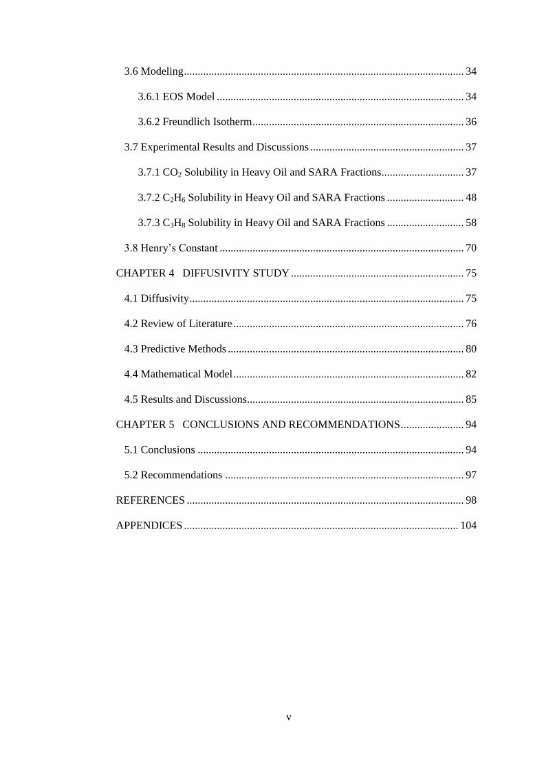
3.6 Modeling ...................................................................................................... 34

3.6.1 EOS Model .......................................................................................... 34

3.6.2 Freundlich Isotherm ............................................................................. 36

3.7 Experimental Results and Discussions ........................................................ 37

3.7.1 CO2 Solubility in Heavy Oil and SARA Fractions .............................. 37

3.7.2 C2H6 Solubility in Heavy Oil and SARA Fractions ............................ 48

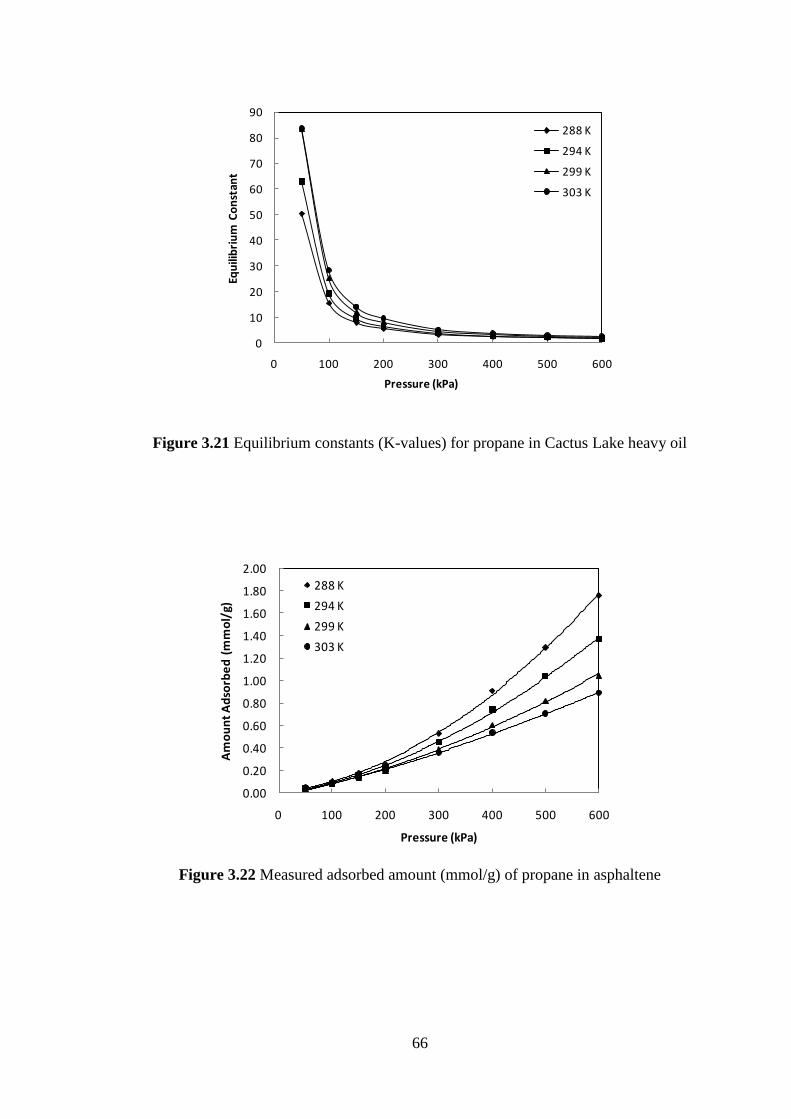
3.7.3 C3H8 Solubility in Heavy Oil and SARA Fractions ............................ 58

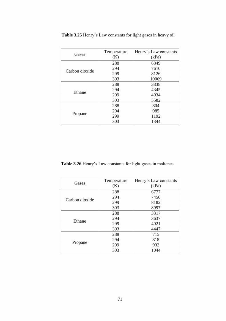
3.8 Henry‟s Constant ......................................................................................... 70

CHAPTER 4 DIFFUSIVITY STUDY ............................................................... 75

4.1 Diffusivity .................................................................................................... 75

4.2 Review of Literature .................................................................................... 76

4.3 Predictive Methods ...................................................................................... 80

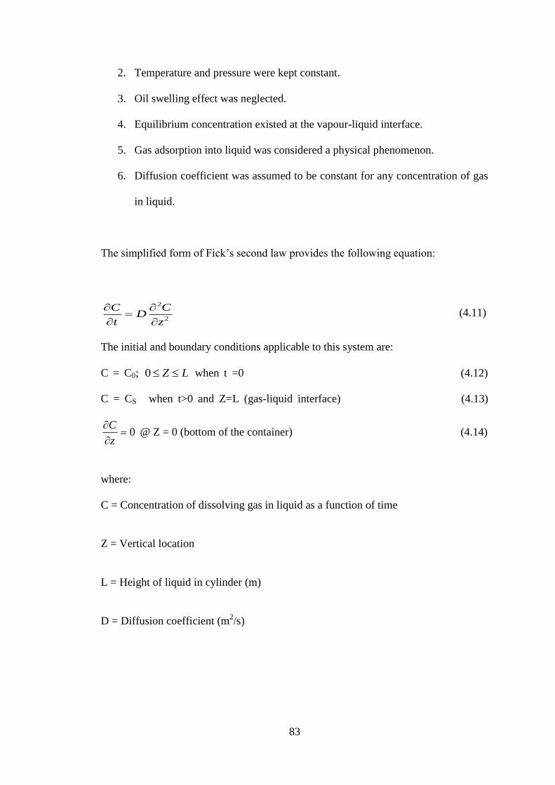
4.4 Mathematical Model .................................................................................... 82

4.5 Results and Discussions ............................................................................... 85

CHAPTER 5 CONCLUSIONS AND RECOMMENDATIONS ....................... 94

5.1 Conclusions ................................................................................................. 94

5.2 Recommendations ....................................................................................... 97

REFERENCES ..................................................................................................... 98

APPENDICES .................................................................................................... 104

vi

LIST OF TABLES

Table 2.1 Compositional analysis results of the Cactus Lake Crude Oil .............. 7

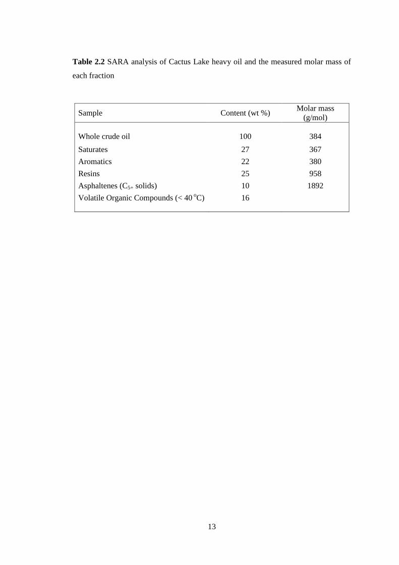
Table 2.2 SARA analysis of Cactus Lake heavy oil and measured molar mass of

each fraction ........................................................................................ 13

Table 2.3 Microbalance components contributing to Buoyancy Calculation ......19

Table 2.4 Comparison of solubility of C02-Hexadecane System ........................19

Table 3.1

Parameters for cubic equations of state ...............................................32

Table 3.2

Parameter definition for two cubic EOS ..............................................32

Table 3.3

Critical properties calculated for PR-EOS ...........................................35

Table 3.4

Measured solubility (wt. %) of carbon dioxide in heavy oil ...............40

Table 3.5

Measured solubility (wt. %) of carbon dioxide in maltene .................41

Table 3.6

Measured solubility (wt. %) of carbon dioxide in saturate fraction ....42

Table 3.7

Measured solubility (wt. %) of carbon dioxide in aromatic fraction ...43

Table 3.8

Measured solubility (wt. %) of carbon dioxide in resin fraction .........44

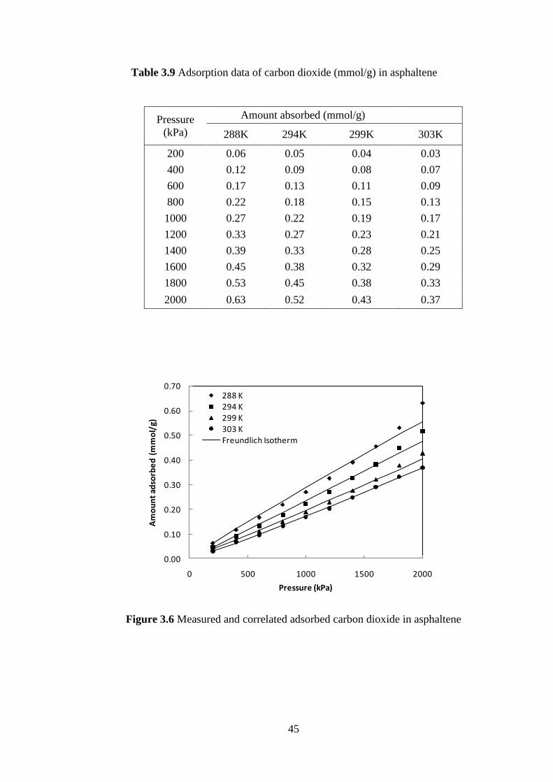
Table 3.9

Measured adsorption data of carbon dioxide

(mmol/g) in asphaltene ........................................................................45

Table 3.10

Peng-Robinson interaction parameters and deviations ........................ 46

Table 3.11

Measured solubility (wt %) of ethane in heavy oil .............................. 50

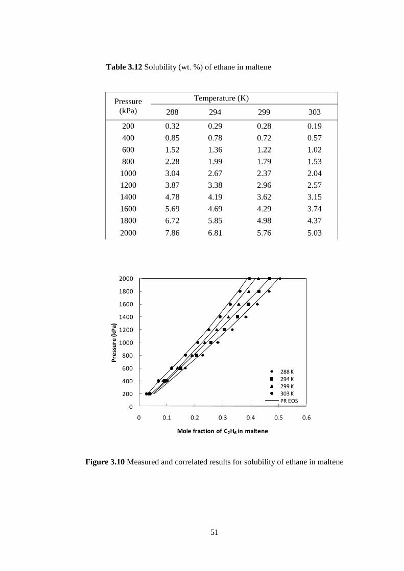
Table 3.12

Measured solubility (wt %) of ethane in maltene ................................ 51

Table 3.13

Measured solubility (wt %) of ethane in saturate fraction ................... 52

Table 3.14

Measured solubility (wt %) of ethane in aromatic fraction ................. 53

Table 3.15

Measured solubility (wt %) of ethane in resin fraction 54

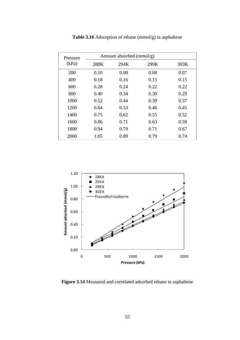
Table 3.16

Measured adsorption data of ethane (mmol/g) in asphaltene .............. 55

Table 3.17

Peng-Robinson interaction parameters and deviations ........................ 56

Table 3.18

Measured solubility (wt %) of propane in heavy oil ........................... 61

Table 3.19 Measured solubility (wt %) of propane in maltene ............................. 62

vii

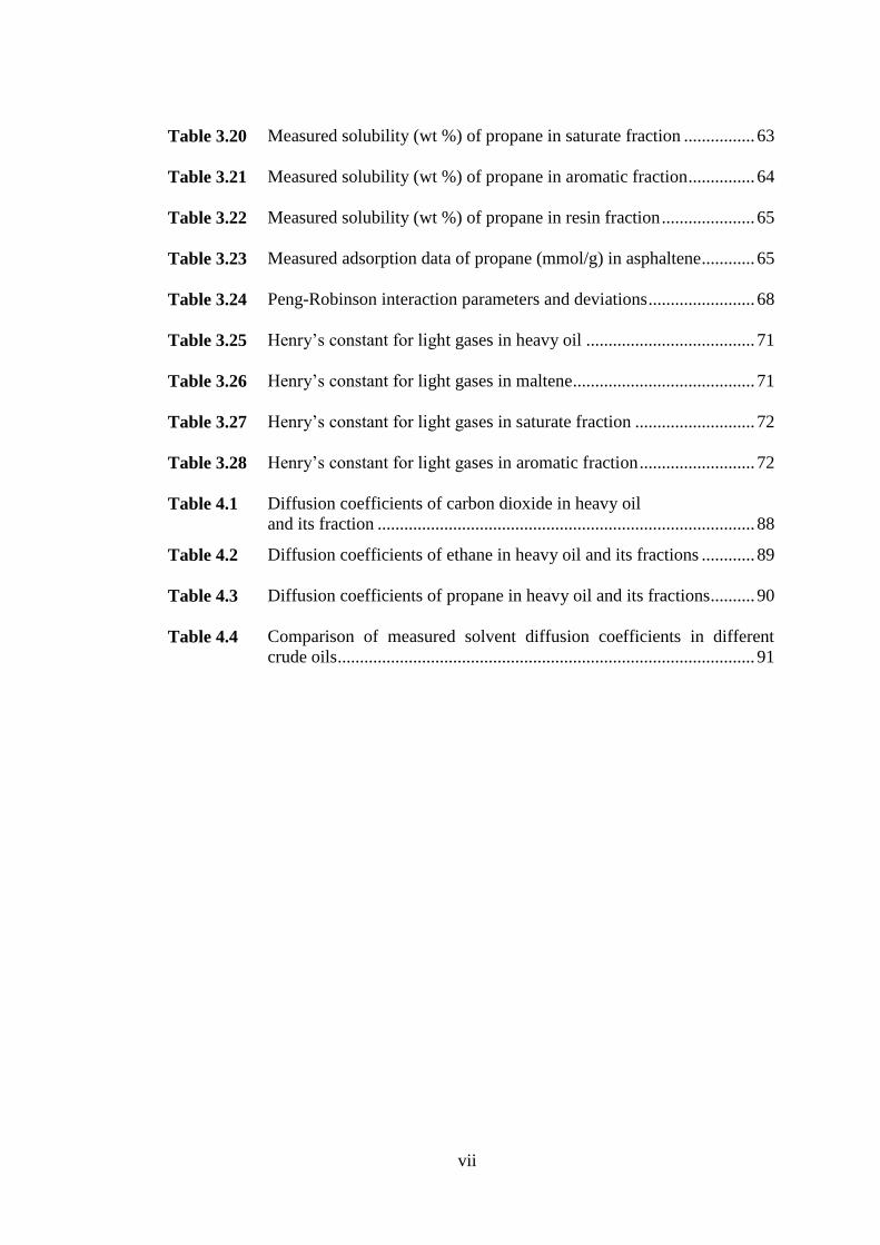
Table 3.20

Measured solubility (wt %) of propane in saturate fraction ................ 63

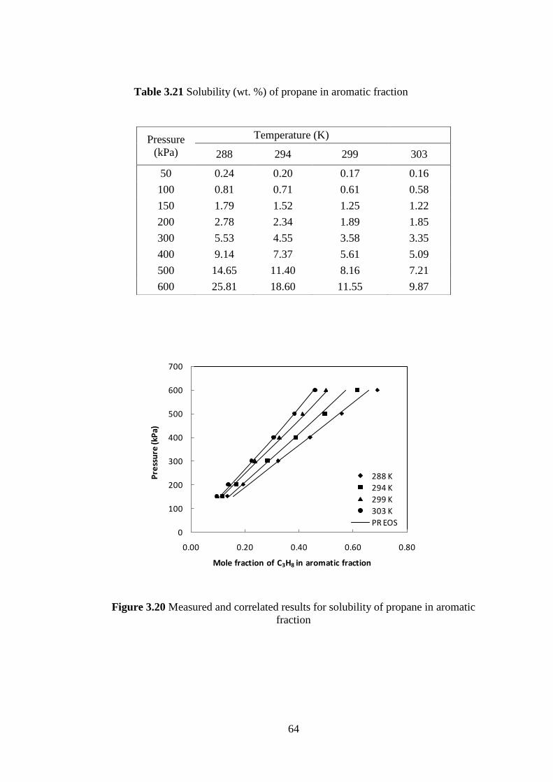
Table 3.21

Measured solubility (wt %) of propane in aromatic fraction ............... 64

Table 3.22

Measured solubility (wt %) of propane in resin fraction ..................... 65

Table 3.23

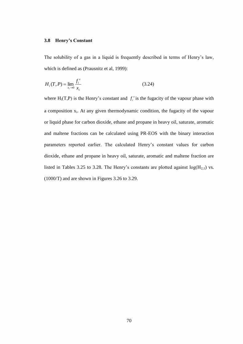
Measured adsorption data of propane (mmol/g) in asphaltene ............ 65

Table 3.24

Peng-Robinson interaction parameters and deviations ........................ 68

Table 3.25

Henry‟s constant for light gases in heavy oil ...................................... 71

Table 3.26

Henry‟s constant for light gases in maltene ......................................... 71

Table 3.27

Henry‟s constant for light gases in saturate fraction ........................... 72

Table 3.28

Henry‟s constant for light gases in aromatic fraction .......................... 72

Table 4.1

Diffusion coefficients of carbon dioxide in heavy oil

and its fraction ..................................................................................... 88

Table 4.2

Diffusion coefficients of ethane in heavy oil and its fractions ............ 89

Table 4.3

Diffusion coefficients of propane in heavy oil and its fractions .......... 90

Table 4.4

Comparison of measured solvent diffusion coefficients in different

crude oils .............................................................................................. 91

viii

LIST OF FIGURES

Figure 2.1 SARA Separation flow diagram ....................................................... 9

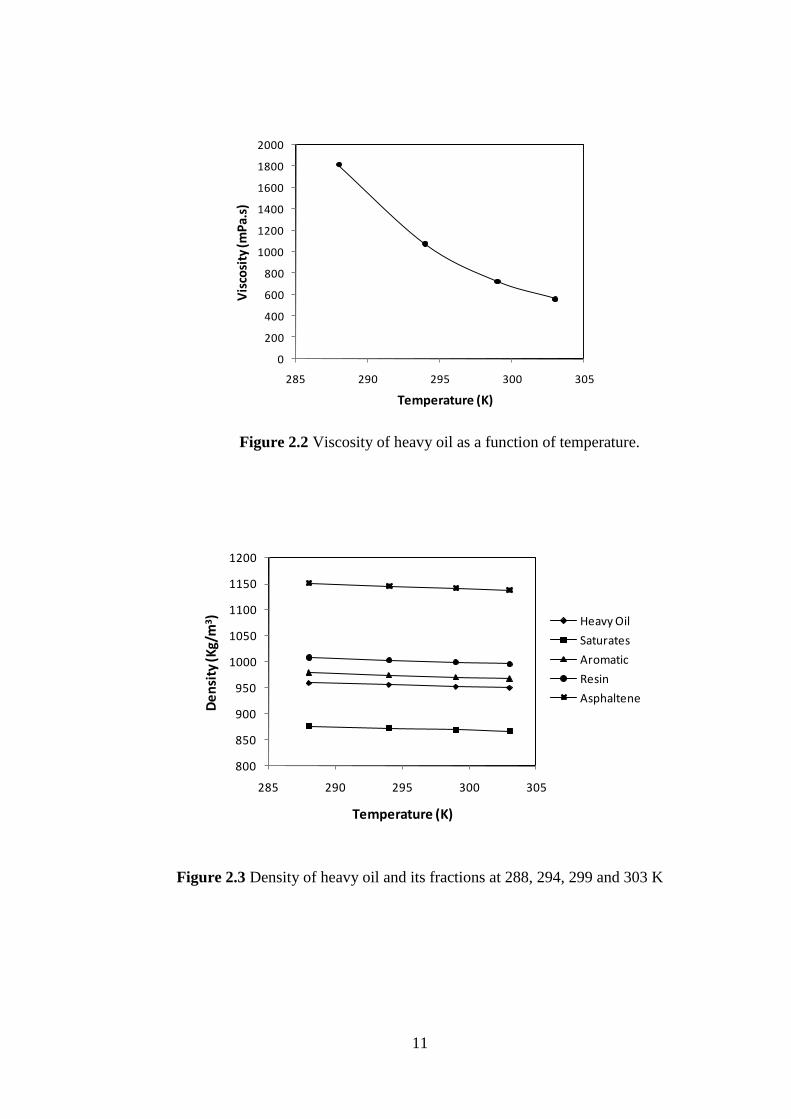
Figure 2.2 Viscosity of heavy oil as a function of temperature ......................... 11

Figure 2.3 Density of heavy oil and its fractions at temperatures 288, 294, 299

and 303 K ......................................................................................... 11

Figure 2.4 Schematic diagram of intelligent gravimetric microbalance (IGA

003) .................................................................................................. 15

Figure 2.5 Microbalance for solubility and diffusivity measurement ............... 16

Figure 2.6 Solubility of CO2 in Hexadecane ..................................................... 20

Figure 3.1 Measured and correlated results for solubility of carbon dioxide in

heavy oil ........................................................................................... 40

Figure 3.2 Measured and correlated results for solubility of carbon dioxide in

maltene ............................................................................................. 41

Figure 3.3 Measured and correlated results for solubility of carbon dioxide in

saturate fraction ................................................................................ 42

Figure 3.4 Measured and correlated results for solubility of carbon dioxide in

aromatic fraction .............................................................................. 43

Figure 3.5 Measured and correlated results for solubility of carbon dioxide in

resin fraction..................................................................................... 44

Figure 3.6 Measured and correlated adsorbed carbon dioxide in asphaltene ... .45

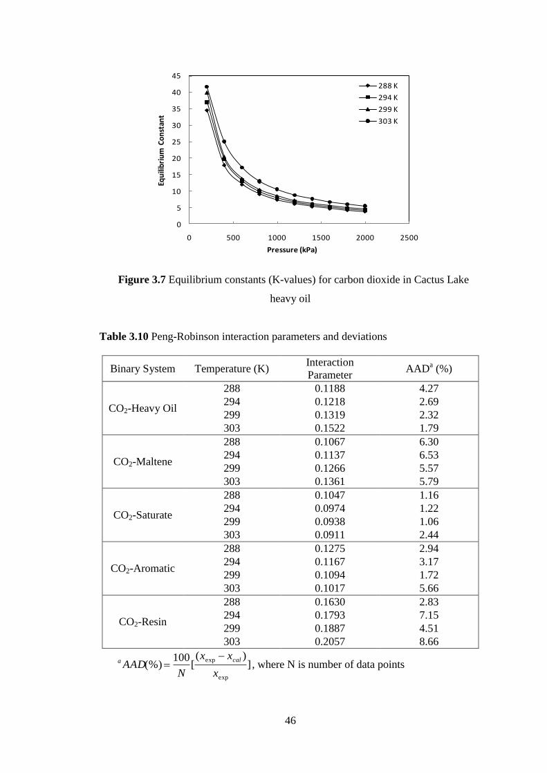
Figure 3.7 Equilibrium constants (K-values) for carbon dioxide in Cactus Lake

heavy oil ........................................................................................... 46

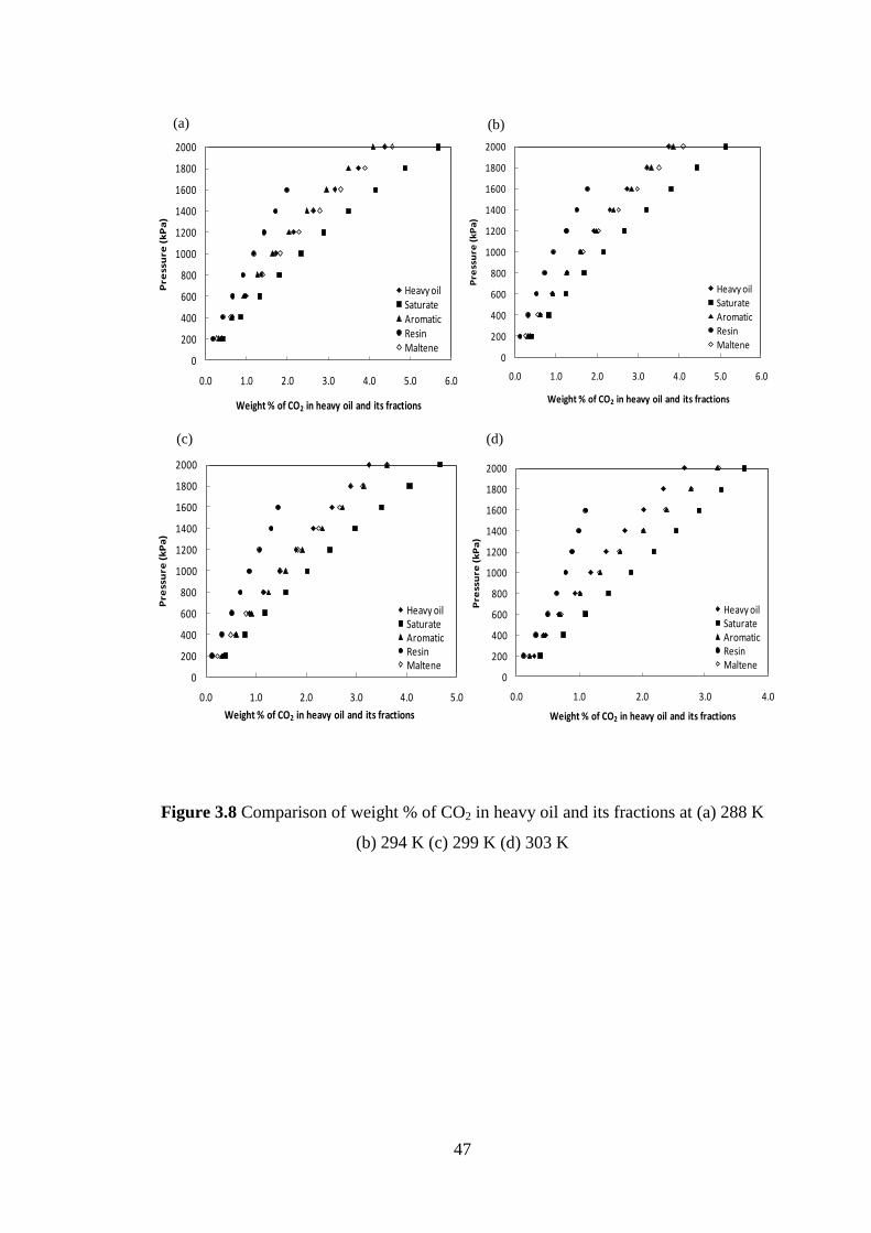
Figure 3.8 Comparison of Weight % of CO2 in heavy oil and its fractions at (a)

288 K (b) 294 K (c) 299 K (d) 303 K .............................................. 47

Figure 3.9 Measured and correlated results for solubility of

ethane in heavy oil ........................................................................... 50

Figure 3.10 Measured and correlated results for solubility of

ethane in maltene.............................................................................. 51

Figure 3.11 Measured and correlated results for solubility of ethane in saturate

fraction ............................................................................................. 52

ix

Figure 3.12 Measured and correlated results for solubility of ethane in aromatic

fraction ............................................................................................. 53

Figure 3.13 Measured and correlated results for solubility of ethane in resin

fraction ............................................................................................. 54

Figure 3.14 Measured and correlated adsorbed ethane in asphaltene ................. 55

Figure 3.15 Equilibrium constants (K-values) for ethane in Cactus Lake heavy

oil ..................................................................................................... 56

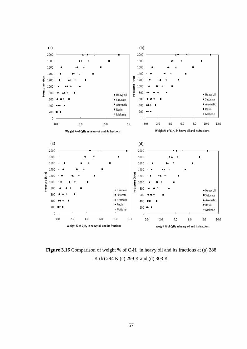
Figure 3.16 Comparison of Weight % of C2H6 in heavy oil and its fractions at (a)

288 K (b) 294 K (c) 299 K and (d) 303 K ........................................ 57

Figure 3.17 Measured and correlated results for solubility of propane in heavy

oil ..................................................................................................... 61

Figure 3.18 Measured and correlated results for solubility of

propane in maltene ........................................................................... 62

Figure 3.19 Measured and correlated results for solubility of propane in saturate

fraction ............................................................................................. 63

Figure 3.20 Measured and correlated results for solubility of propane in aromatic

fraction ............................................................................................. 64

Figure 3.21

Equilibrium constants (K-values) for propane in Cactus Lake heavy

oil ..................................................................................................... 66

Figure 3.22

Measured adsorbed amount (mmol/g) of propane in asphaltene ..... 66

Figure 3.23

Comparison of Weight % of C2H6 in heavy oil and its fractions at (a)

288 K (b) 294 K (c) 299 K and (d) 303 K ........................................ 67

Figure 3.24

Interaction binary parameter, kij, against the temperature for CO2 +

heavy oil (rectangle), C2H6 + heavy oil (circle) and C3H8 + heavy oil

(triangle) ........................................................................................... 68

Figure 3.25

Comparison of amount adsorbed (mmol/g) of CO2, C2H6 and C3H8

in asphaltene at (a) 288 K (b) 294 K (c) 299 K and (d) 303 K ........ 69

Figure 3.26

Henry‟s constants for light gases in heavy oil ................................. 73

Figure 3.27

Henry‟s constants for light gases in maltene ................................... 73

Figure 3.28

Henry‟s constants for light gases in saturate fraction ...................... 74

Figure 3.29

Henry‟s constants for light gases in aromatic fraction ..................... 74

x

Figure 4.1

Schematic of one dimensional diffusion model for solvent-heavy oil

system ............................................................................................... 84

Figure 4.2

Variation of the concentration with time for CO2-heavy oil system at

288 K and 1999.9 kPa ...................................................................... 92

Figure 4.3

Comparison of diffusion coefficients of carbon dioxide in whole oil,

maltene, saturate and aromatic fractions at 1999.9 kPa ................... 92

Figure 4.4

Comparison of diffusion coefficients of ethane in whole oil,

maltene, saturate and aromatic fractions at 1999.8 kPa ................... 93

Figure 4.5

Comparison of diffusion coefficients of propane in whole oil,

maltene, saturate and aromatic fractions at 599.8 kPa ..................... 93

xi

LIST OF APPENDICES

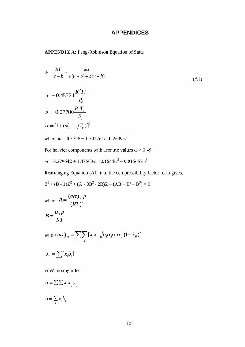
Appendix A Peng-Robinson Equation of state ................................................. 104

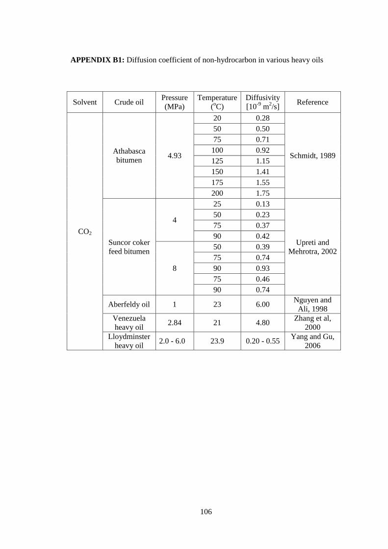
Appendix B1 Diffusion coefficient of non-hydrocarbon in various heavy oils .. 106

Appendix B2 Diffusion coefficient of hydrocarbon in various heavy oils ......... 107

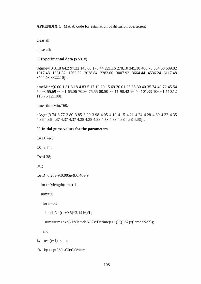
Appendix C Matlab code for estimation of diffusion coefficient ..................... 108

xii

NOMENCLATURE

Notations

Ai

Polynomial coefficient defined in Eq. (2.2)

c Correction term defined in Eq. (3.14)

C1 and C2

Constants defined in Eq. (3.12) and (3.13)

C2

Concentration of the solute defined in Eq. (2.2)

Cu

Concentration of the adsorbed species, mmol/g

D

Molecular diffusivity, m2/sec

ΔE Difference in voltage between the thermistors defined in Eq. (2.2)

v

if Fugacity

F Objective function defined in Eq. (3.19)

Hi(T,P)

Henry‟s constant

k Freundlich constant defined in Eq. (3.20)

k Boltzman constant defined in Eq. (4.4)

ki,j

Binary interaction parameter

K Calibration constant defined in Eq. (2.2)

M Molecular weight, g/mol

M2

Molar mass of the solute defined in Eq. (2.2)

n Freundlich constant defined in Eq. (3.20)

P Pressure, kPa

Pc

Critical pressure, bar

R

Universal gas constant, J/K.mol

rA

radius of diffusion molecule of gas A defined in Eq. (4.4)

SG Specific gravity

xiii

t Time, sec

T

Temperature, K

Tb

Boiling point temperature, K

Tr

Reduced temperature

Tc

Critical temperature, K

vcor

Corrected molar volume defined in Eq. (3.14)

w Weight percentage, wt.%

wasp

Asphaltene weight percentage, wt.%

xi,cal

Calculated mole fraction of oil

xi,meas

Measured mole fraction of oil

Greek Letters

, b, ,

and

Constants defined in Eq. (3.10)

∞ Parameter defined in Eq. (3.7)

ρ Density, Kg/m3

μ Viscosity, mPa.s

ω Pitzer acentric factor

Subscripts

i, j Indices

SARA Saturate, Aromatic, Resin and Asphaltene

1

1. INTRODUCTION

1.1 Enhanced Oil Recovery Techniques

In order to meet future energy demand, better exploitation of heavy oil and bitumen is

necessary. There are abundant resources of bitumen and heavy oil in Canada which

are considered a potential source of petroleum products for the coming years. As

mentioned by Ali (2003), the largest accumulation of heavy oil and tar sand (“oil

sands in Canada”) are in Canada (3 trillion bbls) followed by Venezuela (2 trillion

bbls). The heavy oil is highly viscous (104-10

6 mPa·s or even higher) and thus, an

effective, economical and environmentally friendly recovery process must be

developed to reduce the viscosity of the oil.

In a broad classification, enhanced oil recovery (EOR) techniques include chemical,

thermal and solvent based methods. Chemical EOR processes are mainly alkaline-

surfactant-polymer (ASP) flooding processes. In chemical flooding, the chemicals,

which are made up largely of surfactants, are mixed with water and injected into the

reservoir to increase the oil flow by reducing the interfacial tension between the

injected fluid and in-place crude oil or by altering the wettability of rocks. Polymer

flooding involves the injection of augmented polymers into the reservoir to enhance

the volumetric sweep efficiency by reducing the mobility of injected fluid. One

advantage of polymer flooding is that early breakthrough of injected fluid can be

prevented or avoided. Polymer flooding is limited to light and medium gravity oil

recovery (Wang and Dong, 2007).

At present, thermal based oil recovery methods, such as the steam assisted gravity

2

drainage (SAGD) process (Butler et al, 1981) and the cyclic stream stimulation (CSS)

process (Denbina et al, 1991) are the most commonly used technologies because of

their ability to reduce heavy oil viscosity. The SAGD method was successfully

applied to several projects in Western Canada for the recovery of heavy oil/bitumen.

Due to the requirement of large quantities of energy and water, the SAGD process can

become inefficient and uneconomical. Also CSS and SAGD are energy intensive

processes and are environmentally very unfriendly (Zadeh et al, 2008).

The Vapour Extraction Process (VAPEX) is an alternative to the SAGD process when

4

1.3 Purpose and Scope of this Study

This study covers the measurement and modeling of the solubility and diffusivity of

carbon dioxide, ethane and propane in heavy oil and its maltene, saturate, aromatic,

resin and asphaltene fractions. The objectives of this work are as follows:

1. Based on the molecular structure and molar mass, heavy oil was to be

fractionated into saturate, aromatic, resin, asphaltene and maltene fractions

using the modified ASTM-2007 method.

2. Measurement of the density, viscosity and molar mass of heavy oil, saturate,

aromatic, resin, asphaltene and maltene fractions at temperatures close to the

reservoir temperature.

3. Measurement of the solubility and kinetics of light gases such as carbon

dioxide, ethane and propane in whole heavy oil and in saturate, aromatic,

resin, asphaltene and maltene fractions at 288, 294, 299 and 303 K,

respectively.

4. Tuning the Peng-Robinson equation of state using binary interaction

parameters to correlate the experimental results.

5. Henry‟s constant was calculated for light gases in heavy oil and its maltene,

saturate and aromatic fractions.

6. Adsorbed amount of carbon dioxide and ethane in asphaltene was correlated

using Freundlich isotherm.

7. Estimation of the diffusion coefficients of carbon dioxide, ethane and propane

in heavy oil and its fractions as taken from time-dependent concentration data.

5

1.4 Outline of the Thesis

The thesis is comprised of five chapters. Chapter 1 presents the introduction of the

research together with the purpose and scope of this study. Chapter 2 describes the

experimental set ups and experimental procedures with respect to the tested samples.

Chapter 3 presents experimental and modeling solubility results for the heavy oil and

its fractions. Chapter 4 discusses the diffusivity data obtained using a simple diffusion

model. Finally, Chapter 5 highlights the major works of this thesis and includes some

recommendations for future research.

6

2. EXPERIMENTAL SECTION

2.1 Materials

The original heavy oil sample was collected from the Cactus Lake area, Canada.

Cactus Lake is located in Southwestern Saskatchewan and is comprised of 170

kilometer‟s of crude oil and condensate pipelines and 26,000 barrels of storage. The

system, which has a capacity of 50,000 barrels per day, currently transports

approximately 17,000 barrels per day from regional heavy oil production sites to the

market hub at Kerrobert, Saskatchewan. The density and viscosity of the cleaned field

heavy oil sample was ρoil = 952.15 Kg/m3 and μoil = 724.151 mPa·s at 1 atm and the

reservoir temperature of 299 K, respectively. The compositional analysis of this heavy

oil, obtained using simulated distillation (SIMDIST) analysis, is given in Table 2.1.

As observed in Table 2.1, the mole fraction of C7+ is 0.9876 while the calculated

relative molecular mass and density of C7+ is 392 g/mole and 965.6 kg/m3. The

purities of CO2, C2H6, C3H8 used for this study were 99.99%, 99.90% and 99.99%,

(Praxair Inc., Regina). Sigma Aldrich (Canada) supplied the Hexadecane with a mass

purity of 99.00 %.

2.2 SARA Fractionation

A modified Clay-Gel Absorption Chromatography (ASTM D 2007) method was used

to separate the heavy oil into saturates, aromatics, resins and asphaltenes. The dried

whole sample was dispersed in a 50 fold excess of pentane, gently heated with

agitation, and then cooled to room temperature. The flocculated (precipitated)

asphaltenes were removed by filtration, and the pentane solvent was removed with a

hot plate also set at 308-313 K, overnight. The maltenes were collected accordingly

7

Table 2.1 Compositional analysis of the Cactus Lake crude oil

Carbon Number Mole Fraction Carbon Number Mole Fraction

C1 0.0000 C17 0.0308

C2 0.0000 C18 0.0271

C3 0.0008 C19 0.0301

iC4 0.0012 C20 0.0254

C4 0.0019 C21 0.0236

iC5 0.0050 C22 0.0194

C5 0.0035 C23 0.0200

C6 0.0120 C24 0.0173

C7 0.0161 C25 0.0183

C8 0.0232 C26 0.0162

C9 0.0260 C27 0.0152

C10 0.0322 C28 0.0151

C11 0.0331 C29 0.0162

C12 0.0354 C30+ 0.3865

C13 0.0428 Total 1.00

C14 0.0345 C1 to C6 0.0124

C15 0.0382 C7+ 0.9876

C16 0.0329

8

and evaporated to a constant weight over a hot plate also set at 308-313 K, overnight.

Asphaltene and maltene weights were combined and the percentage loss in mass

relative to the original sample loss was identified as the volatile fraction.

The modified ASTM D2007 was followed in order to separate the maltene fractions

into saturate, aromatic and resin fractions. The maltenes were passed through two

columns of chromatographic separation: an Attapulgite clay-packed column absorbs

the resins and a second column, packed with activated silica gel, separates aromatics

from the saturate fraction. A 50:50 mixture of toluene and acetone was used to

recover the resin fraction from the clay packing. The aromatics can be recovered

using Soxhlet extraction of the silica gel in hot toluene. The entire separation process

is explained in detail as a flow diagram in Figure 2.1 (Speight and Ozum, 2002)

9

Figure 2.1 SARA Separation flow diagram

Resins Oil

Silica gel

Aromatics Saturates

Asphaltene De-asphalted oil

Clay

Heavy Oil

10

2.3 Density and Viscosity Measurements

The densities of the heavy oil, saturate, aromatic and resin fractions were measured at

288, 294, 299 and 303 K, respectively, using a stabinger viscometer (Anton-Parr

SVM 3000) following the ASTM D-7042 method. The reproducibility of the

measurement was 0.0005 g/cc. The density measurements were done with a

precision of ±0.0001 g/cc. The kinematic viscosity of the heavy oil was

simultaneously measured. The viscosity of the heavy oil is shown in Figure 2.2. The

densities of the heavy oil and its fractions are shown in Figure 2.3. The density of

asphaltene was calculated indirectly from the mixing rule given by the following

equation:

SARAi i

i

m

x

1 (2.1)

2.4 Molar Mass Measurements

The average molar mass of the original heavy oil and its two light fractions (saturate

and aromatic) were measured using Cryette A. Cryette A is a precise instrument with

which to measure the molar mass of a substance by tracking freezing point

depression. Cryette A is capable of measuring a freezing point change of 0.001 K.

The molar mass of the other two heavy fractions of heavy oil (resin and asphaltene)

were measured using vapour pressure osmometry (ASTM method D-2503). A vapour

pressure osmometer works on the principle of difference in the vapour pressure

caused by the addition of a small amount of solute to a pure solvent. Within the

vapour pressure osmometer, a small amount of solute-solvent mixture and a small

amount of pure solvent are kept in separate thermistors surrounded by the pure

solvent vapour.

11

0

200

400

600

800

1000

1200

1400

1600

1800

2000

285 290 295 300 305

Vis

cosi

ty (m

Pa.

s)

Temperature (K)

Figure 2.2 Viscosity of heavy oil as a function of temperature.

800

850

900

950

1000

1050

1100

1150

1200

285 290 295 300 305

De

nsi

ty (K

g/m

3 )

Temperature (K)

Heavy Oil

Saturates

Aromatic

Resin

Asphaltene

Figure 2.3 Density of heavy oil and its fractions at 288, 294, 299 and 303 K

12

The difference in the vapour pressure between the two samples provides the

temperature difference between the thermistors. The relation between the molar mass

and the difference in voltage caused by the temperature difference is as follows

(Peramanu et al, 1999):

....)1

( 2

2221

22

CACAM

KC

E (2.2)

Where, E is the difference in voltage between the thermistors, C2 is the

concentration of the solute, K is the calibration constant, M2 is the molar mass of the

solute and Ai are the polynomial coefficients. Calibration was carried out with an

ideal solute-solvent mixture having a low solvent concentration. With regard to the

ideal mixtures, the higher order terms became insignificant and Equation 2.2 could be

written as:

)1

(21

22

CAM

KC

E

(2.3)

The average molar mass of the original oil and its four fractions (SARA) are given in

Table 2.2

13

Table 2.2 SARA analysis of Cactus Lake heavy oil and the measured molar mass of

each fraction

Sample Content (wt %) Molar mass

(g/mol)

Whole crude oil

100

384

Saturates 27 367

Aromatics 22 380

Resins 25 958

Asphaltenes (C5+ solids) 10 1892

Volatile Organic Compounds (< 40 oC) 16

14

2.5 Solubility Measurements

In this study, the gas solubility and diffusivity were made using a gravimetric

microbalance (Hiden Isochema Ltd, IGA 003). IGA 003 can perform absorption-

desorption isotherms and isobar measurements in both static and dynamic mode. In

the dynamic mode, it is possible to have up to four gas streams mixed prior to entry

into the IGA system so that a defined gas mixture composition is delivered at the

sample position. This mode provides a continuous flow of gases (max. 500 cm3

min-1

)

past the sample, and the exhaust valve controls the set point pressure. In this study, all

absorption as well as adsorption measurements were performed in the static mode.

The gas was introduced into the top of the balance, away from the sample, and both

the admittance and exhaust valve control the set-point pressure. As all experiments

were performed by injecting pure hydrocarbons into the system, the static mode was

selected over the dynamic mode for this experiment. It should be noted both the static

and dynamic mode recorded data on a real time basis.

Figure 2.4 shows the experimental set-up used in this study. The major component of

the study is a microbalance consisting of an electro balance with sample and counter

weight components inside a stainless steel pressure vessel. The designed stainless

steel (SS 316L) reactor operates at a maximum pressure and temperature of 2000 kPa

and 773.15 K, respectively. Pressures from 10-7

to 10 kPa were measured using a

capacitance manometer (Pfeiffer, model PKR251), and pressures from 10 to 2000 kPa

were measured using a Piezo-resistive strain gauge (Druck, model PDCR 4010). The

reactor pressure set point was maintained to within 0.4-0.8 kPa.

15

Figure 2.4 Schematic diagram of intelligent gravimetric microbalance (IGA 003)

3i

2i

1i

MFC

A

B

C D

E

F

G

L To Vent

J K

j1

J2

H I

Enlarge picture of the sample

container and counter weight

A-Cabinet, B-Pressure transducer, C-Air

Admittance Valve, D-Muti Flow Controller, E-

Reservoir, F-Water Bath Controller, G-Water

Bath, H-Reactor, I-Counter Weight, J-Cylinder

1, K-Cylinder 2, L-Diaphragm Pump, M-Turbo

molecular pump, N-Weighing mechanism.

31i and j1-2 are explained in Table 2.3

N

M

16

Figure 2.5 Microbalance for solubility and diffusivity measurement

17

Several measurements were taken to ensure the machine was properly calibrated. In

the first experiment, the counter weight was removed and in the second experiment,

the sample container was removed. In both cases a solvent gas (CO2) was introduced

into the reactor. It was found the microbalance components contributing to the

buoyancy calculation, were within an acceptable limit. The major microbalance

components, contributing to the buoyancy calculation, are shown in Table 2.3.

In order to validate the equipment, as reported in the literature, some of the

experimental data were recorded at low pressures and were reproduced for the carbon

dioxide-hexadecane system. The experimental data, presented by Campos et al (2009)

and Amon et al (1986), were used to compare the present data. Table 2.4 shows the

experimental data obtained in the present work for the carbon dioxide + hexadecane

system at 303.2, 308.2 and 313.2 K. Figure 2.6 shows the comparison between the

present study and the literature. The obtained mean deviations were 3.23%, 2.47%

and 6.24% for 303.2 K, 308.2 K and 313.2 K, respectively.

Prior to starting the original experiment, several experiments were conducted in order

to understand the behaviour of the oil. Heavy oil of around 122.43 mg was dried and

the atmospheric gases were evacuated from the reactor using the turbo pump. As soon

as the pressure reached vacuum pressure (8-10 mbar), the turbo pump was closed and

the reactor remained constant at 303.2 K for 30 hours. It was observed the sample

weight was reduced to 121.66 mg representing a reduction in mass of 0.77 mg (0.63%

of its original quantity). The weight loss was attributed to the evaporation of light

volatile components and moisture, etc. Since the experiments were conducted at the

low temperatures of 288, 294, 299 and 303 K and the experimental pressures were

18

above atmospheric pressure, the vaporization of the lighter components at lower

temperatures can be considered within experimental error.

The solubility of carbon dioxide and ethane in heavy oil and its fractions (SARA)

were determined at four different temperatures of 288, 294, 299 and 303 K,

respectively, and at several pressures up to 2000 kPa (200, 400, 600, 800, 1000, 1200,

1400, 1600, 1800 and 2000 kPa) and for propane pressures up to 600 kPa (50, 100,

150, 200, 300, 400, 500 and 600 kPa). Approximately 80-120 mg of samples (the

quantity remains the same for both heavy oil and SARA fractions) were put in a

sample container of 0.59984 g and the reactor was sealed. Then, the experimental

temperature was set using an external water jacket connected to a remote controlled

constant temperature bath (Huber Ministat, model cc-S3). The reactor was degassed,

first using a diaphragm pump (Pfeiffer, model MVP055-3) and then using a turbo

pump (Pfeiffer, model TSH-071). The leak rate of the reactor was less than 10-9

mbar

1/sec and a conflate type copper gasket seals were used to ensure a minimum leak

rate. The samples remained under such conditions for several hours (a minimum of 30

minutes and a maximum of 4 hours depending upon the type of sample) to reach

equilibrium. It was assumed the system has attained equilibrium when no further

changes occurred in the mass of the sample over time. Under the aforementioned

conditions, the solvent gas was introduced into the reactor. To ensure sufficient time

for gas-liquid equilibrium, different samples were maintained at set pressure points

for various times. For the sake of this study, the maximum equilibrium time set for

heavy oil and SARA fractions was 150 minutes for heavy oil, 90 minutes for

saturates, 130 minutes for aromatics and maltenes, 180 minutes for resins and 220

minutes for asphaltenes, respectively.

19

Table 2.3 Microbalance components contributing to the buoyancy calculation

Subscript Item Weight

(gm)

Material Density

(g/ cm3)

Temperature

(K)

S Dry mass ms Heavy Oil ρs Sample

Temp., Ts

a Interacted mass ma CO2 ρa Ts

i1 Sample Container 0.59984 Stainless

Steel

7.393103 322.67

i2 Lower sample

Hang down

0.06524 Tungsten 21 322.67

i3 Upper sample

Hang down

0.3055 Gold 19.8 308.15

j1 Counter Weight 0.81219 Stainless

Steel

7.9 297.60

j2 Upper Counter

Weight Hang down

0.239 Gold 19.8 308.15

Table 2.4 Comparison of solubility of CO2-Hexadecane system

Temperature

(K)

Pressure

(kPa)

Solubility (mole fraction) %

Deviation References

This Study Literature

303.2

51.7 0.007 0.007 0.00

Campos et

al, 2009

106.5 0.016 0.016 0.00

165.4 0.024 0.025 4.17

252.1 0.039 0.041 5.13

355.7 0.058 0.062 6.89

308.2 690.0 0.081 0.083 2.47 Amon et al,

1986

313.2

55.0 0.006 0.005 16.67

Campos et

al, 2009

110.2 0.013 0.012 7.69

169.6 0.021 0.021 0.00

257.0 0.034 0.035 2.94

361.2 0.051 0.053 3.92

20

0

100

200

300

400

500

600

700

800

0.00 0.02 0.04 0.06 0.08 0.10

Pre

ssu

re (k

Pa)

Mole fraction of CO2 in Hexadecane

303.2 K (This study) 303.2 K (Campos et al., 2009)

308.2 K (This study) 308.2 K (Amon et al., 1986)

313.2 K (This study) 313.2 K (Campos et al., 2009)

Figure 2.6 Solubility of CO2 in Hexadecane

21

IGA 003 ensures proper safety of the machine as well as safety to the user. The

prominent safety features include a pressure relief valve and an over temperature

controller arrangement. If the pressure exceeds 2500 kPa (designed pressure 2000

kPa), the pressure relief valve will then open automatically. Again, if the temperature

exceeds 373.15 K, the over temperature interlock controller will ultimately turn off

the water bath.

The reason IGA 003 was selected for this study over other available equipment on the

market was the fact its resolution was very high (0.1 μg). It provides real time data

and was designed in such a way to minimize buoyancy effects. Also, a minimal

amount of sample was required (typically 80-120 mg) as compared to other

equipment (Zadeh et al, 2008 and Upreti and Mehrotra, 2000). Therefore, IGA 003

can measure solubility data very precisely and the measurement of diffusivity takes

significantly less time (typically 90-220 minutes for each pressure set point depending

upon the type of sample).

22

3. SOLUBILITY STUDY

3.1 General Introduction

Gas solubility in a liquid is a thermodynamic property which depends on the type of

gas being dissolved, the type and composition of the liquid, and conditions of

temperature and pressure. It is very important to know the composition of solvent/gas

in liquid reservoirs at a particular pressure and temperature.

3.2 Heavy Oil Characterization

Due to the complex composition of crude oils, characterisation of the individual

molecular types is not possible, and elemental analysis is unattractive because it gives

only limited information about the constitution of petroleum due to the constancy of

elemental composition. Indeed, hydrocarbon group type analysis is commonly

employed (Fan and Buckley, 2002 and Fan et al, 2002). The SARA-separation is an

example of such group type analysis, separating the crude oils into four main

chemical classes based on differences in solubility and polarity. The four SARA

fractions are saturates (S), aromatics (A), resins (R) and asphaltenes (A).

Saturates

The saturates (aliphatics) are non-polar hydrocarbons without double bonds, but

including straight chain and branched alkanes, as well as cycloalkanes (naphtenes).

Cycloalkanes contain one or more rings, which may have several alkyl side chains.

The proportion of saturates in a crude oil normally decrease with increasing molecular

weight fractions and thus, saturates are the lightest fraction of the crude oil.

23

Aromatic

The term “aromatics” refers to benzene and its structural derivates. Aromatics are

common to all petroleum, and by far the majority of aromatics contain alkyl chains

and cycloalkane rings, along with additional aromatic rings. Aromatics are often

classified as mono-, di-, and tri-aromatics depending on the number of aromatic rings

present in the molecule. Polar, higher molecular weight aromatics may fall into the

resin or asphaltene fraction.

Resins

This fraction is comprised of polar molecules often containing heteroatoms such as

nitrogen, oxygen or sulphur. The resin fraction is operationally defined and one

common definition of resins is the fraction is soluble in light alkanes such as pentane

and heptanes, but is insoluble in liquid propane. Since the resins are defined as a

solubility class, overlap of both to the aromatic and the asphaltene fraction is

expected. Despite the fact the resin fraction is very important in regard to crude oil

properties, little work has been reported on the characteristics of the resins as

compared to asphaltenes, for example. However, some general characteristics may be

identified. Resins have a higher H/C ratio than asphaltenes at, 1.2-1.7 compared to

0.9-1.2 for the asphaltenes (Anderson and Speight, 2001). Resins are structurally

similar to asphaltenes, but smaller in molecular weight (<1000 g/mole).

Asphaltenes

Asphaltene could be considered large resins. The highest polar fractions of the crude

oil were the asphaltenes. Asphaltenes undergo self-association, which causes them to

differ from resins. The molecular weight of asphaltene molecules has been difficult to

measure due to the asphaltenes tendency to self-aggregate, but molecular weights in

24

the range of 500-2000 g/mole are believed to be reasonable (Groenzin and Mullins,

2000).

3.3 Empirical Correlations for Critical Properties

The use of an equation of state to predict the phase behaviour of gas in heavy

oil/bitumen is challenging work as it requires the availability of critical properties of

heavy oil. Numerous methods are available and the main application of the methods is

to estimate critical properties of undefined petroleum fractions when experimental

data are not available. Only the three most widely used methods are discussed herein.

Lee-Kesler Method

Kesler and Lee proposed the following correlations to estimate the critical

temperature, critical pressure and acentric factor (Kesler and Lee, 1976):

bbc TSGTSGSGT /10)0069.11441.0()1174.04244.0(6.4508.189 5 (3.1)

310

2

26

2

3

2

10)9099.9

4505.2(10)15302.0

182.147579.0(10)21343.01216.4

43639.0(0566.0689.5ln

bb

bc

TSG

TSG

SGTSGSG

SGP

(3.2)

For Tbr≤0.8

6

6

43577.0ln4721.13/6875.152518.15

169347.0ln28862.1/09648.692714.501325.1/ln

brbrbr

brbrbrc

TTT

TTTP

(3.3)

25

For Tbr>0.8

brwbrww TKTKK /)01063.0408.1(359.800765.01352.0904.7 2 (3.4)

where, Tb and Tc were in Kelvin and Pc in bar.

Twu Method

Twu proposed some correlations for critical properties with a specific gravity and

boiling point as input parameters for heavy hydrocarbons. They used vapor pressure

data to obtain the constants for critical properties correlations. Correlations for critical

temperature and critical pressure are listed below (Twu, 1984):

11324

31023

)106077.4

106584.171052617.21034383.053327.0(

b

bbbbc

Tx

TxTxTxTT (3.5)

2422/1 )35886.275041.91610.931412.000661.1( cP (3.6)

cb TT /1 (3.7)

where, Tb and Tc were in Kelvin and Pc in bar.

Riazi-Daubert Method

Riazi and Daubert recommended simplified correlations with which to estimate the

critical properties for hydrocarbons with molar mass in the range of (70 to 300)

g/gmol. The correlations are given below (Riazi and Daubert, 1980):

53691.08106.044 )]104791.654444.010314.9[exp(5233.9 SGTbTbSGxSGTbxTc

(3.8)

0846.44844.0335 )]10749.58014.410505.8[exp(101958.3 SGTbSGTxSGTbxxPc b

(3.9)

where, Tb and Tc were in Kelvin and Pc in bar.

26

3.4 Review of the Gas-bitumen/Heavy Oil System

Numerous solubility data are available for a heavy oil-light gas system. Simon and

Graue (1965) determined solubility data by measuring the properties of CO2 in nine

different oils at temperatures ranging from (311 to 394) K and pressures of up to 15.9

MPa and developed different graphical correlations. However, the main drawback of

this research was the solubility data were not in mathematical form and, hence could

not be implemented into a computer simulator.

Mehrotra et al (1984) investigated the prediction of thermodynamic properties for

Alberta bitumen using the Peng-Robinson (PR) equation of state. Lumped component

models have been used to depict the phase behavior of gas bitumen mixtures. Five

different correlations were used with the PR equation of state, and it was reported the

Kesler Lee correlations provided better results than other tested correlations.

Fu et al (1985) measured the vapor-liquid properties of carbon dioxide-Athabasca

bitumen and nitrogen-Athabasca bitumen. They used a modified apparatus to measure

the VLE properties. The experiments were carried out at a temperature of 373 K and

pressures from (4.9 to 8.13) MPa for carbon dioxide, and at 403 K for nitrogen at

pressures from (4 to 11.5) MPa. Measured values were compared with values where

the PR and the modified Soave-Redlich-Kwong (SRK) equation of states were used.

They concluded the results were in satisfactory agreement with the literature results.

Schwarz and Prausnitz (1987) measured the solubility of carbon dioxide, methane and

ethane in six characterized heavy fossil fractions. Four fractions were from crude oil

and two fractions were from coal liquid. Solubility was measured at pressures from

27

(5.8 to 21) bar and temperatures from (374 to 575) K. Henry‟s law constants were

calculated from the solubility data using an equation of state.

Saturated Cold Lake bitumen was measured by Mehrotra and Svrcek (1984). It was

reported the gas solubility data were in qualitatively agreement with other Alberta

bitumens. They also measured the properties of bitumen saturated with mixtures of

CO2 and CH4 and found the solubility of the gas mixture also increased with pressure.

Fu et al (1988) measured vapor-liquid equilibrium properties of methane-Cold Lake

bitumen and ethane-Cold Lake bitumen systems. They produced three isotherms for

the pseudo binary systems at 343.2, 373.2 and 423.2 K and at pressures of up to11.9

MPa. A modified SRK equation of state and a PR equation of state were used in this

study to correlate the experimental results. The measured data were in good

agreement with the calculated results.

Yu et al (1989) measured the solubility of supercritical carbon dioxide in bitumen at

temperatures up to 523 K and at pressures up to 16 MPa. They used the Perturbed

Hard Chain (PHC) equation of state to calculate the bitumen phase equilibrium. The

PR equation of state was also used to estimate the binary parameters and they were

compared with the results of the PHC equation of state. It was concluded the PR

binary parameters were systematically higher than the PHC binary parameters.

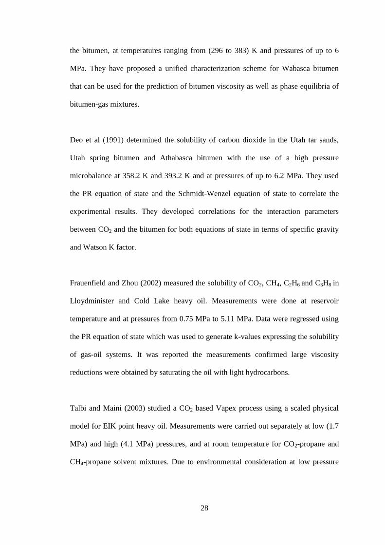
Mehrotra et al (1989) determined the solubility of CO2 in Wabasca bitumen, which

was characterized by three pseudo components representing the distillable maltenes,

un-distillable maltenes and asphaltenes, constituted 45, 43.2 and 11.8 mass percent of

28

the bitumen, at temperatures ranging from (296 to 383) K and pressures of up to 6

MPa. They have proposed a unified characterization scheme for Wabasca bitumen

that can be used for the prediction of bitumen viscosity as well as phase equilibria of

bitumen-gas mixtures.

Deo et al (1991) determined the solubility of carbon dioxide in the Utah tar sands,

Utah spring bitumen and Athabasca bitumen with the use of a high pressure

microbalance at 358.2 K and 393.2 K and at pressures of up to 6.2 MPa. They used

the PR equation of state and the Schmidt-Wenzel equation of state to correlate the

experimental results. They developed correlations for the interaction parameters

between CO2 and the bitumen for both equations of state in terms of specific gravity

and Watson K factor.

Frauenfield and Zhou (2002) measured the solubility of CO2, CH4, C2H6 and C3H8 in

Lloydminister and Cold Lake heavy oil. Measurements were done at reservoir

temperature and at pressures from 0.75 MPa to 5.11 MPa. Data were regressed using

the PR equation of state which was used to generate k-values expressing the solubility

of gas-oil systems. It was reported the measurements confirmed large viscosity

reductions were obtained by saturating the oil with light hydrocarbons.

Talbi and Maini (2003) studied a CO2 based Vapex process using a scaled physical

model for EIK point heavy oil. Measurements were carried out separately at low (1.7

MPa) and high (4.1 MPa) pressures, and at room temperature for CO2-propane and

CH4-propane solvent mixtures. Due to environmental consideration at low pressure

29

and the high recovery rate at high pressure, they recommended CO2-propane mixture

as a suitable Vapex solvent for heavy oil.

Riazi and Vera (2005) proposed the P-N-A compositional model based on regular

solution theory for the estimation of light gases in petroleum fractions at various

pressures and temperatures. They recommended the model could be used directly to

predict the solubility of gases in petroleum mixtures/coal cuts for gas with known

solubility parameters.

Phase behavior and viscosity of butane saturated heavy oil was measured and

modeled by Yazdani and Maini (2007). Each measurement was carried out at 295 K

and at pressures below the vapor pressure of butane. Phase behavior was correlated

using PR-EOS by taking into consideration heavy oil as a single pseudo component

and as two pseudo components.

Badamchizadeh et al (2008) developed a new experimental method to check the

VAPEX process performance for Athabasca bitumen recovery. They measured the

solubility and phase behavior of CO2-Athabasca bitumen, propane-Athabasca bitumen

and CO2-propane bitumen mixtures. Interaction parameters between components were

used as tuning parameters for the PR-EOS and ternary diagram for the predicted CO2-

propane bitumen mixture using the tuned EOS.

Nikookar et al (2008) analyzed the density of some crude oil components based on the

saturates, aromatics, resins and asphaltenes (SARA) method and estimated the density

30

and solubility parameters of different crude oil samples using their proposed equation

of states (EOS).

Badamchizadeh et al (2009) measured the solubility of propane in Athabasca bitumen

and liquid phase densities and viscosities at typical Canadian heavy oil reservoir

temperatures. A modified Raoult‟s law was used to fit the measured saturation

pressure data. It was reported the viscosity reduction in the Vapex process as thermal

methods needing higher solvent fraction in the liquid, which could cause serious

asphaltene deposition.

Luo and Gu (2009) measured the physiochemical properties of propane saturated

heavy oil at 293.95 K and at pressures from (300 to 850) kPa. They reported

asphaltene deposition was not observed at pressures below 780 kPa and deposition

commenced when the pressure was increased to 850 kPa. It was concluded de-

asphalting behavior or propane solvent altered the physiochemical properties of

saturated heavy oil.

3.5 Equation of State

Cubic equations of state (EOS) are commonly used to predict Vapor-Liquid

equilibrium data. The use of EOS for the calculation of hydrocarbon properties has

become widely accepted throughout the petroleum industry. Here, only two equations

of state are considered as they are extensively used in industrial applications. Most

EOS approaches employ a cubic equation of state with the following general form

(Poling et al, 2001):

31

))((

)(

)( 2

VVbV

V

bV

RTP (3.10)

where, depending upon the model, , b, , and may be constants including zero or

may vary with temperature and/or composition.

Note in the above equations, b is a constant and =b. Parameters of the equation of

states differ depending upon the type of equation. The dependence of parameters a

and b on the critical properties of the components is written in the following form:

a = ac(Tr,) (3.11)

ac = C1RTc2 / Pc (3.12)

b = C2RTc / Pc (3.13)

where the parameter was used to add the temperature dependence to a. C1 and C2

are constants depending on the type of EOS. Few correlations are available in the

literature with which to estimate the critical parameters of the heavy oil and their

components.

32

Table 3.1 Parameters for cubic equations of state

Table 3.2 Parameter definition for two cubic EOS

EOS Number of Parameters

Peng and Robinson (PR) 2b - b2

a (Tr) 3: a, b, (1)

Soave Redlich Kwong

(SRK) 2c c

2 a (Tr) 4 to 5: a, b, c, (1-2)

EOS (Tr) C1 C2

PR

(1976) [1+(0.3746+1.5422ω-2.699 ω2)*(1-Tr

0.5)]2 0.0778 0.4572

SRK

(1984) [1+(0.4998+1.5928ω-0.1956 ω2-0.025 ω3)*(1-Tr

0.5)]2 0.0833 0.4218

33

Vapor-Liquid equilibrium can be accurately predicted using an equation of state.

However in a few systems, significant deviations were observed when predicting the

density/molar volume of pure components using a two-parameter equation of state.

The deviation was nearly constant for a wide range of pressure from the critical value.

Hence, a correction factor is included to improve the predicted liquid density values,

and it had no effect on the phase behavior calculations. Peneloux et al (1982)

introduced the volume shift concept, shifting the volume axis as follows:

ccor (3.14)

where cor

is the corrected molar volume and „c‟ is the correction term.

Various types of mixing rules for determining the EOS parameters have been

developed and used for non ideal gas mixtures. The commonly used mixing rule for

hydrocarbons and petroleum mixtures is called the quadratic mixing rule (Riazi,

2005). With regard to mixtures with composition xi and a total of N components, the

following equations were used to calculate a and b for various types of cubic EOS:

ijji

N

j

N

imix axxa

11 (3.15)

ii

N

imix bxb

1 (3.16)

where, a ij was given by the following equation:

)1()( 2/1

ijjiij kaaa (3.17)

For the volume translation c, the mixing rule was the same as for parameter b:

ii

N

imix cxc

1 (3.18)

34

kij is a dimensionless parameter called the binary interaction parameter (BIP), where

kii = 0 and kij = kji. In most hydrocarbon systems kij = 0; however, for the key

hydrocarbon compounds in a mixture with a difference in the size of molecules, the

value of kij was non-zero.

3.6 Modeling

3.6.1 EOS Model

The prediction of phase behaviour of reservoir fluids under actual reservoir conditions

can be done by using an equation of state (EOS). With regard to this study, CMG‟s

Winprop module (Version 2009.10, Computer Modeling Group Ltd., Canada) was

used to model the experimental results with the Peng-Robinson equation of state

(Peng and Robinson, 1976). EOS modeling requires critical pressure, critical

temperature and Pitzer acentric factor for each fluid component. The above mentioned

requirements are difficult to meet in actual practice due to the extremely complicated

composition of heavy oil. Therefore, a five component system has been modelled in

this work by characterizing the original heavy oil (component #1) into maltene

(component #2), saturate (component #3), aromatic (component #4) and resin

(component #5) fractions. The aforementioned characterizations were conducted

based on the molar mass and the molecular structure of the fractions. Winprop

calculated the critical properties of heavy oil, maltene, saturate, aromatic and resin

fractions using the Lee-Kesler correlation (Kesler and Lee, 1976). The critical

parameters for heavy oil, maltene, saturate, aromatic, resin and the solvent used for

this study are summarized in Table 3.3.

35

Table 3.3 Critical properties calculated for PR-EOS

Component Critical Pressure

(KPa)

Critical Temperature

(K)

Acentric Factor

Heavy Oil 1162.3 910.1 1.05

Maltene 1182.8 906.4 1.04

Saturate 993.7 859.5 1.03

Aromatic 1230.6 918.78 1.02

Resin 527.3 1067.03 1.55

CO2 7376.4 304.2 0.225

C2H6 4883.8 305.4 0.098

C3H8 4245.5 369.8 0.152

36

In all systems (solvent-heavy oil, solvent-maltene, solvent-saturates, solvent-aromatic

and solvent-resin) the binary interaction coefficients were selected as tuning

parameters to regress the experimental pressures. The regression was performed by

minimizing the following objective function (CMG, 2009):

i

measimeasicalcii xxxwF 2

,,, ]/)([ (3.19)

where, xi,calc and xi,meas correspond to the calculated value and measured value,

respectively. The weights wi are used to assign a degree of importance to each data

point. The default value is 1.0. A larger value gives more importance to the data while

a lesser value gives less importance.

3.6.2 Freundlich Isotherm

The asphaltene and solvent system was modelled using Freundlich equation (Do,

1998) which takes the following forms:

n

u kPC /1 (3.20)

where, Cu is the concentration of the adsorbed species (mmol/g) and k and n are

generally temperature dependent. The Freundlich constant n indicates the degree of

favorability of adsorption and should have values lying in the range of 1 to 10 so as to

classify as favourable adsorption. Another constant k is used to estimate the enthalpy

of adsorption. From the enthalpy of adsorption, the spontaneity and nature of

adsorption, as to whether it is exothermic or endothermic, is predicted. A smaller

value of (1/n) indicates a stronger bond between adsorbate and adsorbent, while a

higher value for k indicates the rate of adsorbate removal is high (Proctor and

Vazquez, 1996). Parameters of the Freundlich equation can be found by plotting

)(log10 uC versus )(log10 P .

37

)(log1

)(log)(log 101010 Pn

kCu (3.21)

which yields a straight line with a slope of (1/n) and an intercept of )(log10 k

3.7 Experimental Results and Discussion

3.7.1 CO2 Solubility in Heavy Oil and SARA Fraction

Solubilities of carbon dioxide in heavy oil and in saturate, aromatic, resin, asphaltene

and maltene fractions were measured at 288, 294, 299 and 303 K, respectively. The

experimental results are reported in Tables 3.4 to 3.9.

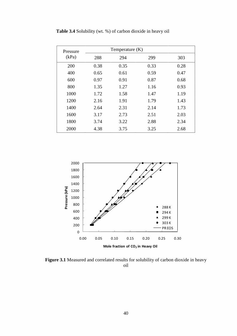
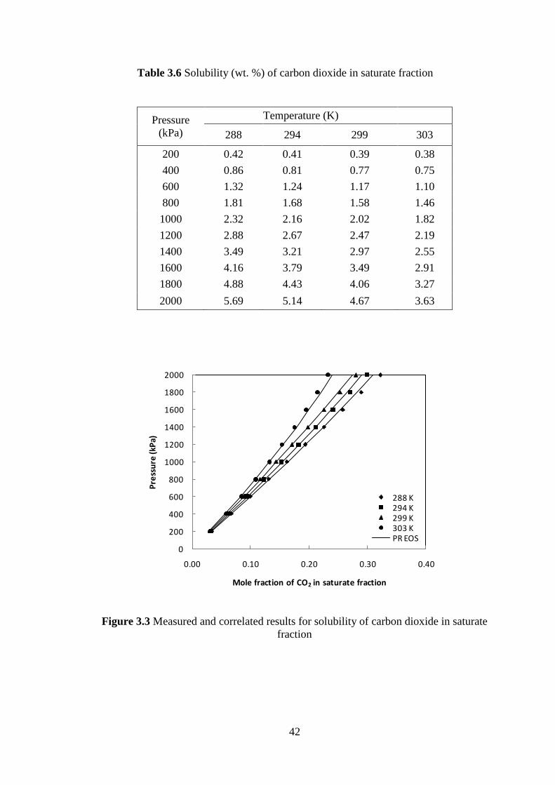
Solubility of CO2 in heavy oil and its fractions increased with increasing pressure at

constant temperature and decreased with increasing temperature. Figures 3.1 to 3.5

show the measured (symbols) and calculated (lines) solubilities of CO2 in heavy oil

and in maltene, saturate, aromatic and resin fractions at pressures ranging from 200

kPa to 2000 kPa. CO2 solubilities calculated from the Winprop module with the PR-

EOS and a regression were carried out by selecting binary interaction parameters as

tuning parameters to optimize the measured pressures of all four temperatures. The

optimized binary interaction coefficients for each system are reported in Table 3.10.

Two-phase flash calculation was used to determine the K-values at each pressure

within isothermal conditions and the results are shown in Figure 3.7. The average

deviation of CO2 solubility between the measured and correlated results in heavy oil,

maltene, saturate, aromatic and resin fractions were 2.76%, 6.04%, 1.47%, 3.37% and

5.78%, respectively. Measured solubility of CO2 in heavy oil and its fractions at low

pressure (below 200 kPa), for all experimental temperatures, were considered

unreliable, because the data points did not obey Henry‟s law when compared to high

38

pressure data. Also, PR-EOS was not able to correlate the data points within

acceptable deviations.

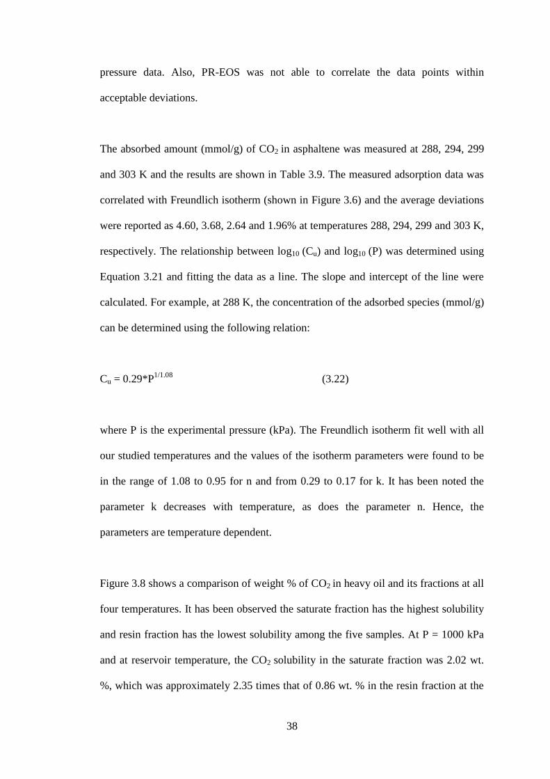
The absorbed amount (mmol/g) of CO2 in asphaltene was measured at 288, 294, 299

and 303 K and the results are shown in Table 3.9. The measured adsorption data was

correlated with Freundlich isotherm (shown in Figure 3.6) and the average deviations

were reported as 4.60, 3.68, 2.64 and 1.96% at temperatures 288, 294, 299 and 303 K,

respectively. The relationship between log10 (Cu) and log10 (P) was determined using

Equation 3.21 and fitting the data as a line. The slope and intercept of the line were

calculated. For example, at 288 K, the concentration of the adsorbed species (mmol/g)

can be determined using the following relation:

Cu = 0.29*P1/1.08

(3.22)

where P is the experimental pressure (kPa). The Freundlich isotherm fit well with all

our studied temperatures and the values of the isotherm parameters were found to be

in the range of 1.08 to 0.95 for n and from 0.29 to 0.17 for k. It has been noted the

parameter k decreases with temperature, as does the parameter n. Hence, the

parameters are temperature dependent.

Figure 3.8 shows a comparison of weight % of CO2 in heavy oil and its fractions at all

four temperatures. It has been observed the saturate fraction has the highest solubility

and resin fraction has the lowest solubility among the five samples. At P = 1000 kPa

and at reservoir temperature, the CO2 solubility in the saturate fraction was 2.02 wt.

%, which was approximately 2.35 times that of 0.86 wt. % in the resin fraction at the

39

same conditions, which was approximately 1.37 times that of 1.47 wt. % when

compared to the original heavy oil.

40

Table 3.4 Solubility (wt. %) of carbon dioxide in heavy oil

0

200

400

600

800

1000

1200

1400

1600

1800

2000

0.00 0.05 0.10 0.15 0.20 0.25 0.30

Pre

ssu

re (k

Pa)

Mole fraction of CO2 in Heavy Oil

288 K

294 K

299 K

303 K

PR EOS

Figure 3.1 Measured and correlated results for solubility of carbon dioxide in heavy

oil

Pressure

(kPa)

Temperature (K)

288 294 299 303

200 0.38 0.35 0.33 0.28

400 0.65 0.61 0.59 0.47

600 0.97 0.91 0.87 0.68

800 1.35 1.27 1.16 0.93

1000 1.72 1.58 1.47 1.19

1200 2.16 1.91 1.79 1.43

1400 2.64 2.31 2.14 1.73

1600 3.17 2.73 2.51 2.03

1800 3.74 3.22 2.88 2.34

2000 4.38 3.75 3.25 2.68

41

Table 3.5 Solubility (wt. %) of carbon dioxide in maltene

0

200

400

600

800

1000

1200

1400

1600

1800

2000

0.000 0.050 0.100 0.150 0.200 0.250 0.300

Pre

ssu

re (k

Pa)

Mole fraction of CO2 in maltene

288 K

294 K

299 K

303 K

PR-EOS

Figure 3.2 Measured and correlated results for solubility of carbon dioxide in maltene

Pressure

(kPa)

Temperature (K)

288 294 299 303

200 0.27 0.25 0.21 0.20

400 0.62 0.56 0.49 0.43

600 0.99 0.89 0.79 0.72

800 1.41 1.26 1.13 1.01

1000 1.82 1.66 1.47 1.32

1200 2.29 2.04 1.83 1.64

1400 2.80 2.52 2.24 2.02

1600 3.32 2.98 2.66 2.38

1800 3.91 3.50 3.12 2.79

2000 4.57 4.10 3.60 3.22

42

Table 3.6 Solubility (wt. %) of carbon dioxide in saturate fraction

0

200

400

600

800

1000

1200

1400

1600

1800

2000

0.00 0.10 0.20 0.30 0.40

Pre

ssu

re (k

Pa)

Mole fraction of CO2 in saturate fraction

288 K294 K299 K303 KPR EOS

Figure 3.3 Measured and correlated results for solubility of carbon dioxide in saturate

fraction

Pressure

(kPa)

Temperature (K)

288 294 299 303

200 0.42 0.41 0.39 0.38

400 0.86 0.81 0.77 0.75

600 1.32 1.24 1.17 1.10

800 1.81 1.68 1.58 1.46

1000 2.32 2.16 2.02 1.82

1200 2.88 2.67 2.47 2.19

1400 3.49 3.21 2.97 2.55

1600 4.16 3.79 3.49 2.91

1800 4.88 4.43 4.06 3.27

2000 5.69 5.14 4.67 3.63

43

Table 3.7 Solubility (wt. %) of carbon dioxide in aromatic fraction

0

200

400

600

800

1000

1200

1400

1600

1800

2000

0.00 0.05 0.10 0.15 0.20 0.25 0.30

Pre

ssu

re (k

Pa)

Mole fraction of CO2 in aromatic fraction

288 K294 K299 K303 KPR EOS

Figure 3.4 Measured and correlated results for solubility of carbon dioxide in

aromatic fraction

Pressure

(kPa)

Temperature (K)

288 294 299 303

200 0.32 0.32 0.32 021

400 0.63 0.61 0.61 0.43

600 0.92 0.92 0.91 0.69

800 1.26 1.26 1.25 1.02

1000 1.63 1.61 1.59 1.34

1200 2.03 1.98 1.93 1.65

1400 2.47 2.39 2.33 2.02

1600 2.95 2.84 2.73 2.39

1800 3.49 3.32 3.15 2.78

2000 4.09 3.85 3.61 3.20

44

Table 3.8 Solubility (wt. %) of carbon dioxide in resin fraction

0

200

400

600

800

1000

1200

1400

1600

1800

0.00 0.10 0.20 0.30 0.40

Pre

ssu

re (k

Pa)

Mole fraction of CO2 in resin fraction

288 K

294 K

299 K

303 K

PR-EOS

Figure 3.5 Measured and correlated results for solubility of carbon dioxide in resin

fraction

Pressure

(kPa)

Temperature (K)

288 294 299 303

200 0.18 0.12 0.12 0.11

400 0.41 0.31 0.31 0.31

600 0.66 0.51 0.51 0.49

800 0.92 0.72 0.68 0.64

1000 1.18 0.93 0.86 0.78

1200 1.43 1.25 1.07 0.89

1400 1.71 1.51 1.29 0.99

1600 1.99 1.76 1.43 1.10

45

Table 3.9 Adsorption data of carbon dioxide (mmol/g) in asphaltene

0.00

0.10

0.20

0.30

0.40

0.50

0.60

0.70

0 500 1000 1500 2000

Am

ou

nt

adso

rbe

d (

mm

ol/

g)

Pressure (kPa)

288 K294 K299 K303 KFreundlich Isotherm

Figure 3.6 Measured and correlated adsorbed carbon dioxide in asphaltene

Pressure

(kPa)

Amount absorbed (mmol/g)

288K 294K 299K 303K

200 0.06 0.05 0.04 0.03

400 0.12 0.09 0.08 0.07

600 0.17 0.13 0.11 0.09

800 0.22 0.18 0.15 0.13

1000 0.27 0.22 0.19 0.17

1200 0.33 0.27 0.23 0.21

1400 0.39 0.33 0.28 0.25

1600 0.45 0.38 0.32 0.29

1800 0.53 0.45 0.38 0.33

2000 0.63 0.52 0.43 0.37

46

0

5

10

15

20

25

30

35

40

45

0 500 1000 1500 2000 2500

Equ

ilib

riu

m C

on

stan

t

Pressure (kPa)

288 K

294 K

299 K

303 K

Figure 3.7 Equilibrium constants (K-values) for carbon dioxide in Cactus Lake

heavy oil

Table 3.10 Peng-Robinson interaction parameters and deviations

Binary System Temperature (K) Interaction

Parameter AAD

a (%)

CO2-Heavy Oil

288 0.1188 4.27

294 0.1218 2.69

299 0.1319 2.32

303 0.1522 1.79

CO2-Maltene

288 0.1067 6.30

294 0.1137 6.53

299 0.1266 5.57

303 0.1361 5.79

CO2-Saturate

288 0.1047 1.16

294 0.0974 1.22

299 0.0938 1.06

303 0.0911 2.44

CO2-Aromatic

288 0.1275 2.94

294 0.1167 3.17

299 0.1094 1.72

303 0.1017 5.66

CO2-Resin

288 0.1630 2.83

294 0.1793 7.15

299 0.1887 4.51

303 0.2057 8.66

])(

[100

(%)exp

exp

x

xx

NAAD

cala

, where N is number of data points

47

Figure 3.8 Comparison of weight % of CO2 in heavy oil and its fractions at (a) 288 K

(b) 294 K (c) 299 K (d) 303 K

0

200

400

600

800

1000

1200

1400

1600

1800

2000

0.0 1.0 2.0 3.0 4.0 5.0 6.0

Pre

ssu

re (

kP

a)

Weight % of CO2 in heavy oil and its fractions

Heavy oilSaturateAromaticResinMaltene

(a)

0

200

400

600

800

1000

1200

1400

1600

1800

2000

0.0 1.0 2.0 3.0 4.0 5.0 6.0

Pre

ssu

re (

kP

a)

Weight % of CO2 in heavy oil and its fractions

Heavy oilSaturateAromaticResinMaltene

(b)

0

200

400

600

800

1000

1200

1400

1600

1800

2000

0.0 1.0 2.0 3.0 4.0 5.0

Pre

ssu

re (

kP

a)

Weight % of CO2 in heavy oil and its fractions

Heavy oilSaturateAromaticResinMaltene

(c)

0

200

400

600

800

1000

1200

1400

1600

1800

2000

0.0 1.0 2.0 3.0 4.0

Pre

ssu

re (

kP

a)

Weight % of CO2 in heavy oil and its fractions

Heavy oilSaturateAromaticResinMaltene

(d)

48

3.7.2 C2H6 Solubility in Heavy Oil and SARA Fraction

Solubilities of ethane in heavy oil and in saturate, aromatic, resin, asphaltene and

maltene fractions were measured at 288, 294, 299 and 303 K. The experimental

results are reported in Tables 3.11 to 3.16.

Solubility of ethane in heavy oil and its fractions increased with increasing pressure at

constant temperature and decreased with increasing temperature. Figures 3.9 to 3.13

show the measured (symbols) and calculated (lines) solubilities of ethane in heavy oil

and in maltene, saturate, aromatic and resin fractions at pressures ranging from 200

kPa to 2000 kPa. Ethane solubilities calculated from the Winprop module with the PR-

EOS and a regression were carried out in order to optimize the measured pressures for

all four temperatures by selecting binary interaction parameters as tuning parameters.

The optimized binary interaction coefficients, for each system, are reported in Table

3.17. Two-phase flash calculation was used to determine the K-values at each

pressure within isothermal conditions and the results are shown in Figure 3.15. The

average deviation of ethane solubility between the measured and correlated results in

heavy oil, maltene, saturate, aromatic and resin fractions were 4.85%, 6.41%, 4.15%,

5.36% and 9.48%, respectively. The experimental data were well correlated for the

ethane-saturate system with no interactions between the gas and liquid. No

interactions would occur if the molecular shape and size of the components were

similar in nature. A higher interaction coefficient between ethane and resin indicates a

poor adsorption of ethane in resin fraction.

The absorbed amount (mmol/g) of ethane in asphaltene was measured at 288, 294,

299 and 303 K and the results are shown in Table 3.16. The measured adsorption data

49

was correlated using Freundlich isotherm (Figure 3.14) and the average deviations

were reported as 7.08, 6.78, 3.64 and 1.97% at 288, 294, 299 and 303 K, respectively.

The relationship between log10(Cu) and log10(P) was determined using Equation 3.21

and fitting the data as a line. The slope and intercept of the line were calculated. As an

example, at 288 K, the concentration of the adsorbed species (mmol/g) can be

determined using the following relation:

Cu = 0.51*P1/1.05

(3.23)

where, P is the experimental pressure (kPa). The Freundlich isotherm fits well with all

our studied temperatures and the values of the isotherm parameters were found in the

range of 1.05 to 1.02 for n and from 0.51 to 0.37 for k. It has been noted the parameter

k decreases with temperature, as does the parameter n. Hence, the parameters are

temperature dependent.

Figure 3.16 shows the comparison of weight % of ethane in heavy oil and its fractions

at all four temperatures. It has been observed the saturate fraction has the highest

solubility and resin fraction has the lowest solubility among the five samples. At P =

1600 kPa and at reservoir temperature, the ethane solubility in the saturate fraction

was approximately 7.24 wt. %, which was about 7.78 times that of 0.93 wt. % in the

resin fraction and within the same conditions, were approximately 2.26 times that of

3.21 wt. % when compared to the original heavy oil. The asphaltene content affects

the ethane solubility in heavy oil at the same equilibrium pressure. For example, when

the equilibrium pressure was recorded as 1600 kPa, the ethane solubility in the

maltene (wasp= 0.0 wt. %) was found to be 4.29 wt. %, which was approximately 1.34

times that of 3.21 wt. % in the original heavy oil (wasp= 10.0 wt. %).

50

Table 3.11 Solubility (wt. %) of ethane in heavy oil

0

500

1000

1500

2000

2500

0.00 0.10 0.20 0.30 0.40 0.50

Pre

ssu

re (k

Pa)

Mole fraction of C2H6 in heavy oil

288 K

294 K

299 K

303 K

PR EOS

Figure 3.9 Measured and correlated results for solubility of ethane in heavy oil

Pressure

(kPa)

Temperature (K)

288 294 299 303

200 0.19 0.15 0.11 0.08

400 0.59 0.48 0.38 0.30

600 1.12 0.89 0.69 0.55

800 1.72 1.42 1.16 0.96

1000 2.32 1.94 1.63 1.38

1200 2.88 2.41 2.01 1.69

1400 3.65 3.08 2.61 2.23

1600 4.43 3.76 3.21 2.77

1800 5.25 4.44 3.77 3.22

2000 6.40 5.33 4.43 3.72

51

Table 3.12 Solubility (wt. %) of ethane in maltene

0

200

400

600

800

1000

1200

1400

1600

1800

2000

0 0.1 0.2 0.3 0.4 0.5 0.6

Pre

ssu

re (k

Pa)

Mole fraction of C2H6 in maltene

288 K294 K299 K303 KPR EOS

Figure 3.10 Measured and correlated results for solubility of ethane in maltene

Pressure

(kPa)

Temperature (K)

288 294 299 303

200 0.32 0.29 0.28 0.19

400 0.85 0.78 0.72 0.57

600 1.52 1.36 1.22 1.02

800 2.28 1.99 1.79 1.53

1000 3.04 2.67 2.37 2.04

1200 3.87 3.38 2.96 2.57

1400 4.78 4.19 3.62 3.15

1600 5.69 4.69 4.29 3.74

1800 6.72 5.85 4.98 4.37

2000 7.86 6.81 5.76 5.03

52

Table 3.13 Solubility (wt. %) of ethane in saturate fraction

0

200

400

600

800

1000

1200

1400

1600

1800

2000

0 0.1 0.2 0.3 0.4 0.5 0.6 0.7

Pre

ssu

re (k

Pa)

Mole fraction of C2H6 in saturate fraction

288 K

294 K

299 K

303 K

PR EOS

Figure 3.11 Measured and correlated results for solubility of ethane in saturate

fraction

Pressure

(kPa)

Temperature (K)

288 294 299 303

200 0.84 0.76 0.68 0.65

400 1.75 1.58 1.48 1.40

600 2.63 2.44 2.34 2.30

800 3.74 3.39 3.24 3.11

1000 4.85 4.35 4.14 3.76

1200 6.00 5.42 5.09 4.42

1400 7.55 6.62 6.17 5.39

1600 9.10 7.81 7.24 6.37

1800 10.83 9.18 8.44 7.36

2000 12.78 10.69 9.58 8.51

53

Table 3.14 Solubility (wt. %) of ethane in aromatic fraction

0

200

400

600

800

1000

1200

1400

1600

1800

2000

0 0.1 0.2 0.3 0.4 0.5

Pre

ssu

re (k

Pa)

Mole fraction of C2H6 in aromatic fraction

288 K

294 K

299 K

303 K

PR EOS

Figure 3.12 Measured and correlated results for solubility of ethane in aromatic

fraction

Pressure

(kPa)

Temperature (K)

288 294 299 303

200 0.08 0.07 0.06 0.05

400 0.41 0.39 0.38 0.37

600 0.87 0.79 0.73 0.69

800 1.41 1.28 1.17 1.09

1000 1.95 1.77 1.62 1.49

1200 2.62 2.35 2.11 1.93

1400 3.35 2.99 2.69 2.45

1600 4.07 3.63 3.27 2.97

1800 4.77 4.28 3.86 3.53

2000 5.48 4.95 4.52 4.17

54

Table 3.15 Solubility (wt. %) of ethane in resin fraction

0

200

400

600

800

1000

1200

1400

1600

1800

0 0.05 0.1 0.15 0.2 0.25 0.3

Pre

ssu

re (k

Pa)

Mole fraction of C2H6 in resin fraction

288 K

294 K

299 K

303 K

PR EOS

Figure 3.13 Measured and correlated results for solubility of ethane in resin fraction

Pressure

(kPa)

Temperature (K)

288 294 299 303

200 0.07 0.06 0.05 0.04

400 0.17 0.16 0.14 0.12

600 0.27 0.25 0.22 0.20

800 0.39 0.36 0.33 0.30

1000 0.53 0.49 0.44 0.39

1200 0.69 0.64 0.58 0.53

1400 0.89 0.81 0.75 0.69

1600 1.08 1.03 0.93 0.84

55

Table 3.16 Adsorption of ethane (mmol/g) in asphaltene

0.00

0.20

0.40

0.60

0.80

1.00

1.20

0 500 1000 1500 2000

Am

ou

nt

adso

rbe

d (

mm

ol/

g)

Pressure (kPa)

288 K294 K299 K303 KFreundlich Isotherm

Figure 3.14 Measured and correlated adsorbed ethane in asphaltene

Pressure

(kPa)

Amount absorbed (mmol/g)

288K 294K 299K 303K

200 0.10 0.08 0.08 0.07

400 0.18 0.16 0.15 0.15

600 0.28 0.24 0.22 0.22

800 0.40 0.34 0.30 0.29

1000 0.52 0.44 0.39 0.37

1200 0.64 0.53 0.46 0.45

1400 0.75 0.62 0.55 0.52

1600 0.86 0.71 0.63 0.59

1800 0.94 0.79 0.71 0.67

2000 1.05 0.89 0.79 0.74

56

0

5

10

15

20

25

30

0 500 1000 1500 2000 2500

Equ

ilib

riu

m C

on

stan

t

Pressure (kPa)

288 K

294 K

299 K

303 K

Figure 3.15 Equilibrium constants (K-values) for ethane in Cactus Lake heavy oil

Table 3.17 Peng-Robinson interaction parameters and deviations

Binary System Temperature (K) Interaction

Parameter AAD

a (%)

C2H6-Heavy Oil

288 0.0649 3.16

294 0.0715 5.29

299 0.0818 5.86

303 0.0944 5.10

C2H6-Maltene

288 0.0347 7.57

294 0.0406 7.18

299 0.0424 6.20

303 0.0544 4.71

C2H6-Saturate

288 0.00 3.89

294 0.00 3.81

299 0.00 3.82

303 0.00 5.08

C2H6-Aromatic

288 0.0739 4.58

294 0.0742 3.77

299 0.0751 4.34

303 0.0765 8.77

C2H6-Resin

288 0.1724 7.92

294 0.1832 9.20

299 0.1896 10.28

303 0.1986 10.53

])(

[100

(%)exp

exp

x

xx

NAAD

cala

, where N is number of data points

57

Figure 3.16 Comparison of weight % of C2H6 in heavy oil and its fractions at (a) 288

K (b) 294 K (c) 299 K and (d) 303 K

0

200

400

600

800

1000

1200

1400

1600

1800

2000

0.0 5.0 10.0 15.0

Pre

ssu

re (

kP

a)

Weight % of C2H6 in heavy oil and its fractions

Heavy oil

Saturate

Aromatic

Resin

Maltene

(a)

0

200

400

600

800

1000

1200

1400

1600

1800

2000

0.0 2.0 4.0 6.0 8.0 10.0 12.0

Pre

ssu

re (

kP

a)

Weight % of C2H6 in heavy oil and its fractions

Heavy oil

Saturate

Aromatic

Resin

Maltene

(b)

0

200

400

600

800

1000

1200

1400

1600

1800

2000

0.0 2.0 4.0 6.0 8.0 10.0

Pre

ssu

re (

kP

a)

Weight % of C2H6 in heavy oil and its fractions

Heavy oil

Saturate

Aromatic

Resin

Maltene

(c)

0

200

400

600

800

1000

1200

1400

1600

1800

2000

0.0 2.0 4.0 6.0 8.0 10.0

Pre

ssu

re (

kP

a)

Weight % of C2H6 in heavy oil and its fractions

Heavy oil

Saturate

Aromatic

Resin

Maltene

(d)

58

3.7.3 C3H8 Solubility in Heavy Oil and SARA Fraction

Solubilities of propane in heavy oil and in saturate, aromatic, resin, asphaltene and

maltene fractions were measured at 288, 294, 299 and 303 K. The experimental

results are reported in Tables 3.18 to 3.22.

Solubility of propane in heavy oil and its fractions increased with increasing pressure

at constant temperature and decreased with increasing temperature. Figure 3.17 to

3.20 shows the measured (symbols) and calculated (lines) solubilities of propane in

heavy oil and in maltene, saturate and aromatic fractions at pressures ranging from 50

kPa to 600 kPa. Propane solubilities, calculated from the Winprop module with the

PR-EOS and a regression were carried out in order to optimize the measured

pressures for all four temperatures by selecting binary interaction parameters as

tuning parameters. The optimized binary interaction coefficients, for each system, are

reported in Table 3.24. Two phase flash calculation was used to determine the K-

values at each pressure within isothermal conditions and the results are shown in

Figure 3.21. The average deviation of propane solubility between the measured and

correlated results in heavy oil, maltene, saturate and aromatic fractions were 6.29%,

2.87%, 5.22%, and 5.37%, respectively. Measured solubility of propane in heavy oil

at low pressures (below 100 kPa), for all experimental temperatures, were considered

unreliable, because the data points did not obey Henry‟s law when compared to high

pressure data. Also, PR-EOS was not able to correlate the data points within

acceptable deviations.

Propane has a very high solubility in saturate fraction and the measured values

correlated with no interaction between the gas and liquid. The propane-resin system

59

was not correlated using PR-EOS for all four temperatures within an acceptable

deviation. It was inferred, via experimental data, propane was appreciably soluble in

resin fraction and may have caused the formation of two liquid phases at pressures

above 400 kPa and at all experimental temperatures. At the end of each experiment, it

was noticed propane highly swelled the resin fraction, causing self-association of

solids, which promoted precipitation. The procedure used and the design of the IGA

did not allow for the measurement of the solubility in each liquid phase. More data

would be necessary to correlate the two-phase system.

The absorbed amount (mmol/g) of propane in asphaltene was measured at 288, 294,

299 and 303 K and the results are shown in Figure 3.22. Figure 3.23 shows a

comparison of weight % of propane in heavy oil and its fractions at all four

temperatures. It has been observed the saturate fraction has the highest solubility and

resin fraction has the lowest solubility among the five samples. For example, at P =

400 kPa and at reservoir temperature, the propane solubility in the saturate fraction

was 10.11 wt. %, which was approximately 14.2 times that of 0.71 wt. % in the resin

fraction and at the same conditions was about 2.1 times that of 4.94 wt. % when

compared to the original heavy oil. The asphaltene content affects the propane

solubility in heavy oil at the same equilibrium pressure. For example, when the

equilibrium pressure was recorded as 400 kPa, the propane solubility in the maltene

(wasp= 0.0 wt. %) was found to be 7.71 wt. %, which was approximately 1.6 times that

of 4.94 wt. % in the original heavy oil (wasp= 10.0 wt. %).

Solubility of propane in heavy oil and its fractions is much higher in comparison to

ethane and carbon dioxide. It can also be observed from the calculated optimized

60

binary interaction parameter using the PR-EOS. Figure 3.24 shows the comparison of

interaction binary coefficient, kij, against the temperatures for CO2 + heavy oil, C2H6

+ heavy oil and C3H8 + heavy oil system. The higher interaction coefficient values for

CO2 in heavy oil indicates less solubility for the system; where-as a low interaction

coefficient value for C3H8 in heavy oil indicates higher solubility for the system.

Adsorption of light gases in asphaltene can be studied by extracting asphaltene from

crude oil and then injecting light gases in asphaltene at different pressures. Dudasova

et al (2008) found a correlation between the amount of nitrogen in the asphaltene

sample and its adsorbed amount on the particle. Similar observations were conducted

by Clementz (1976), where the author studied adsorption of asphaltenes and resins

onto montmorillonite. But, in this research, light gases were injected into the

asphaltene at different pressures and temperatures in order to understand the

adsorption capability of asphaltene in light gases. Figure 3.25 shows the comparison

of the amount of adsorbed (mmol/g) carbon dioxide, ethane and propane in asphaltene

on different pressures (up to 2000 kPa for carbon dioxide and ethane and up to 600

kPa for propane) and at different temperatures from 288 K to 303 K.

61

Table 3.18 Solubility (wt. %) of propane in heavy oil

0

100

200

300

400

500

600

700

0.00 0.20 0.40 0.60 0.80

Pre

ssu

re (k

Pa)

Mole fraction of C3H8 in heavy oil

288 K

294 K

299 K

303 K

PR EOS

Figure 3.17 Measured and correlated results for solubility of propane in heavy oil

Pressure

(kPa)

Temperature (K)

288 294 299 303

50 0.23 0.19 0.14 0.14

100 0.79 0.63 0.47 0.42

150 1.72 1.36 1.05 0.89

200 2.64 2.11 1.63 1.35

300 5.44 4.27 3.14 2.70

400 9.03 6.98 4.94 4.27

500 14.65 10.96 7.29 6.11

600 26.64 18.40 10.66 8.52

62

Table 3.19 Solubility (wt. %) of propane in maltene

0

100

200

300

400

500

600

700

0.00 0.20 0.40 0.60 0.80

Pre

ssu

re (k

Pa)

Mole fraction of C3H8 in maltene

288 K

294 K

299 K

303 K

PR EOS

Figure 3.18 Measured and correlated results for solubility of propane in maltene

Pressure

(kPa)

Temperature (K)

288 294 299 303

50 0.70 0.53 0.51 0.35

100 1.52 1.24 1.23 0.93

150 2.79 2.24 2.11 1.68

200 4.06 3.24 2.98 2.43

300 7.42 5.83 5.13 4.25

400 12.08 9.24 7.71 6.40

500 19.30 14.17 10.98 9.05

600 34.51 23.47 15.43 12.43

63

Table 3.20 Solubility (wt. %) of propane in saturate fraction

0

100

200

300

400

500

600

0.00 0.20 0.40 0.60 0.80 1.00

Pre

ssu

re (k

Pa)

Mole fraction of C3H8 in saturate fraction

288 K

294 K

299 K

303 K

PR-EOS

Figure 3.19 Measured and correlated results for solubility of propane in saturate

fraction

Pressure

(kPa)

Temperature (K)

288 294 299 303

50 0.99 0.89 0.80 0.78

100 2.33 2.03 1.76 1.70

150 3.96 3.39 2.88 2.71

200 5.58 4.75 4.01 3.72

300 9.87 8.25 6.75 6.07

400 15.88 12.96 10.11 8.89

500 25.67 20.00 14.45 12.39

600 47.01 33.60 20.45 16.95

64

Table 3.21 Solubility (wt. %) of propane in aromatic fraction

0

100

200

300

400

500

600

700

0.00 0.20 0.40 0.60 0.80

Pre

ssu

re (k

Pa)

Mole fraction of C3H8 in aromatic fraction

288 K

294 K

299 K

303 K

PR EOS

Figure 3.20 Measured and correlated results for solubility of propane in aromatic

fraction

Pressure

(kPa)

Temperature (K)

288 294 299 303

50 0.24 0.20 0.17 0.16

100 0.81 0.71 0.61 0.58

150 1.79 1.52 1.25 1.22

200 2.78 2.34 1.89 1.85

300 5.53 4.55 3.58 3.35

400 9.14 7.37 5.61 5.09

500 14.65 11.40 8.16 7.21

600 25.81 18.60 11.55 9.87

65

Table 3.22 Solubility (wt. %) of propane in resin fraction

Table 3.23 Adsorption data of propane (mmol/g) in asphaltene

Pressure

(kPa)

Temperature (K)

288 294 299 303

50 0.01 0.01 0.01 0.01

100 0.05 0.04 0.04 0.04

150 0.12 0.10 0.09 0.08

200 0.19 0.17 0.15 0.13

300 0.48 0.39 0.33 0.28

400 1.13 0.90 0.71 0.56

Pressure

(kPa)

Amount absorbed (mmol/g)

288K 294K 299K 303K

50 0.05 0.04 0.03 0.03

100 0.10 0.09 0.07 0.07

150 0.18 0.15 0.13 0.14

200 0.25 0.22 0.19 0.19

300 0.53 0.45 0.38 0.36

400 0.91 0.74 0.60 0.53

500 1.29 1.04 0.82 0.71

600 1.76 1.37 1.05 0.89

66

0

10

20

30

40

50

60

70

80

90

0 100 200 300 400 500 600

Equ

ilib

riu

m C

on

stan

t

Pressure (kPa)

288 K

294 K

299 K

303 K

Figure 3.21 Equilibrium constants (K-values) for propane in Cactus Lake heavy oil

0.00

0.20

0.40

0.60

0.80

1.00

1.20

1.40

1.60

1.80

2.00

0 100 200 300 400 500 600

Am

ou

nt

Ad

sorb

ed

(m

mo

l/g)

Pressure (kPa)

288 K

294 K

299 K

303 K

Figure 3.22 Measured adsorbed amount (mmol/g) of propane in asphaltene

67

Figure 3.23 Comparison of weight % of C3H8 in heavy oil and its fractions at (a) 288

K (b) 294 K (c) 299 K and (d) 303 K

0

100

200

300

400

500

600

0.0 10.0 20.0 30.0 40.0 50.0

Pre

ssu

re (

kP

a)

Weight % of C3H8 in heavy oil and its fractions

Heavy oil

Saturate

Aromatic

Resin

Maltene

(a)

0

100

200

300

400

500

600

0.0 10.0 20.0 30.0 40.0P

ress

ure

(k

Pa

)

Weight % of C3H8 in heavy oil and its fractions

Heavy oil

Saturate

Aromatic

Resin

Maltene

(b)

0

100

200

300

400

500

600

0.0 5.0 10.0 15.0 20.0 25.0

Pre

ssu

re (

kP

a)

Weight % of C3H8 in heavy oil and its fractions

Heavy oil

Saturate

Aromatic

Resin

Maltene

(c)

0

100

200

300

400

500

600

0.0 5.0 10.0 15.0 20.0

Pre

ssu

re (

kP

a)

Weight % of C3H8 in heavy oil and its fractions

Heavy oil

Saturate

Aromatic

Resin

Maltene

(d)

68

Table 3.24 Peng-Robinson interaction parameters and deviations

Binary System Temperature (K) Interaction

Parameter AAD

a (%)

C3H8-Heavy Oil

288 0.0246 4.19

294 0.0291 7.77

299 0.0315 7.01

303 0.0432 6.19

288 0.0061 2.23

C3H8-Maltene 294 0.0073 2.56

299 0.0098 2.02

303 0.0116 4.68

C3H8-Saturate

288 0.00 4.05

294 0.00 5.54

299 0.00 4.48

303 0.00 6.83

C3H8-Aromatic

288 0.0335 5.28

294 0.0314 7.86

299 0.0295 4.29

303 0.0271 4.06

])(

[100

(%)exp

exp

x

xx

NAAD

cala

,where N is number of data point

0

0.02

0.04

0.06

0.08

0.1

0.12

0.14

0.16

285 290 295 300 305

Kij

T/K

Carbon dioxide

Ethane

Propane

Figure 3.24 Binary interaction parameter, kij, against the temperature for CO2 + heavy

oil (rectangle), C2H6 + heavy oil (circle) and C3H8 + heavy oil (triangle)

69

Figure 3.25 Comparison of amount adsorbed (mmol/g) of CO2, C2H6 and C3H8 in

asphaltene at (a) 288 K (b) 294 K (c) 299 K and (d) 303 K

0.00

0.20

0.40

0.60

0.80

1.00

1.20

1.40

1.60

1.80

2.00

0 500 1000 1500 2000 2500

Am

ou

nt a

dso

rb

ed

(m

mo

l/g

)

Pressure (kPa)

Carbon dioxide

Ethane

Propane

(a)

0.00

0.20

0.40

0.60

0.80

1.00

1.20

1.40

1.60

0 500 1000 1500 2000 2500A

mo

un

t a

dso

rbe

d (

mm

ol/

g)

Pressure (kPa)

Carbon dioxide

Ethane

Propane

(b)

0.00

0.20

0.40

0.60

0.80

1.00

1.20

0 500 1000 1500 2000 2500

Am

ou

nt

ad

sorb

ed

(m

mo

l/g

)

Pressure (kPa)

Carbon dioxideEthanePropane

(c)

0.00

0.10

0.20

0.30

0.40

0.50

0.60

0.70

0.80

0.90

1.00

0 500 1000 1500 2000 2500

Am

ou

nt

ad

sorb

ed

(m

mo

l/g

)

Pressure (kPa)

Carbon dioxideEthanePropane

(d)

70

3.8 Henry’s Constant

The solubility of a gas in a liquid is frequently described in terms of Henry‟s law,

which is defined as (Prausnitz et al, 1999):

i

v

i

xi

x

fPTH

i 0lim),(

(3.24)

where Hi(T,P) is the Henry‟s constant and v

if is the fugacity of the vapour phase with

a composition xi. At any given thermodynamic condition, the fugacity of the vapour

or liquid phase for carbon dioxide, ethane and propane in heavy oil, saturate, aromatic

and maltene fractions can be calculated using PR-EOS with the binary interaction

parameters reported earlier. The calculated Henry‟s constant values for carbon

dioxide, ethane and propane in heavy oil, saturate, aromatic and maltene fraction are

listed in Tables 3.25 to 3.28. The Henry‟s constants are plotted against log(H2,1) vs.

(1000/T) and are shown in Figures 3.26 to 3.29.

71

Table 3.25 Henry‟s Law constants for light gases in heavy oil

Gases Temperature

(K)

Henry‟s Law constants

(kPa)

Carbon dioxide

288 6849

294 7610

299 8126

303 10069

Ethane

288 3838

294 4345

299 4934

303 5582

Propane

288 804

294 985

299 1192

303 1344

Table 3.26 Henry‟s Law constants for light gases in maltenes

Gases Temperature

(K)

Henry‟s Law constants

(kPa)

Carbon dioxide

288 6777

294 7450

299 8182

303 8997

Ethane

288 3317

294 3637

299 4021

303 4447

Propane

288 715

294 818

299 932

303 1044

72

Table 3.27 Henry‟s Law constants for light gases in saturate fraction

Gases Temperature

(K)

Henry‟s Law constants

(kPa)

Carbon dioxide

288 5907

294 6322

299 6718

303 6969

Ethane

288 2543

294 2683

299 2765

303 2929

Propane

288 649

294 726

299 835

303 899

Table 3.28 Henry‟s Law constants for light gases in aromatic fraction

Gases Temperature

(K)

Henry‟s Law constants

(kPa)

Carbon dioxide

288 7050

294 7603

299 8003

303 8949

Ethane

288 4176

294 4531

299 4889

303 5232

Propane

288 802

294 925

299 1108

303 1217

73

2.5

2.7

2.9

3.1

3.3

3.5

3.7

3.9

4.1

4.3

4.5

3.3 3.3 3.4 3.4 3.5 3.5

log(

H2

,1)

[kP

a]

1000/T [K-1]

Carbon dioxide

Ethane

Propane

Figure 3.26 Henry‟s Law constants for light gases in heavy oil

2.5

2.7

2.9

3.1

3.3

3.5

3.7

3.9

4.1

4.3

4.5

3.3 3.3 3.4 3.4 3.5 3.5

log(

H2

,1)

[kP

a]

1000/T [K-1]

Carbon dioxide

Ethane

Propane

Figure 3.27 Henry‟s Law constants for light gases in maltene

74

2.5

2.7

2.9

3.1

3.3

3.5

3.7

3.9

4.1

4.3

4.5

3.3 3.3 3.4 3.4 3.5 3.5

log(

H2

,1)

[kP

a]

1000/T [K-1]

Carbon dioxide

Ethane

Propane

Figure 3.28 Henry‟s Law constants for light gases in saturate fraction

2.5

2.7

2.9

3.1

3.3

3.5

3.7

3.9

4.1

4.3

4.5

3.3 3.3 3.4 3.4 3.5 3.5

log(

H2

,1)

[kP

a]

1000/T [K-1]

Carbon dioxide

Ethane

Propane

Figure 3.29 Henry‟s Law constant for light gases in aromatic fraction

75

4. DIFFUSIVITY STUDY

4.1 Diffusivity

Diffusion is the random movement of molecules of a specific species from a high

concentration region to a low concentration region. The mathematical theory of

diffusion in isotropic substances is therefore based on the hypothesis that the rate of

transfer of a diffusion substance through a unit area of a section is proportional to the

concentration gradient measured as normal to the section. This is known as Fick‟s

first law and is given by:

x

CDF

(4.1)

where F is the rate of transfer per unit area of the section, C is the concentration of

diffusing substance, x is the space coordinate measured as normal to the section and D

is called the diffusion coefficient. Equation 4.1 is valid only for an isotropic medium

but is not valid for an anisotropic medium for which the diffusion properties depend

upon the direction in which they are measured. In that situation, the following

equation is applicable:

x

C

x

CD

xt

C

* (4.2)

where, v is molar average velocity. For a system within a stationary closed vessel, the

molar average velocity is zero and therefore the second term on the right hand side of

Equation 4.2 disappears. Thus, Equation 4.2 can be simplified to:

2

2

x

CD

t

C

(4.3)

Mathematically, this equation is usually called the mass transfer diffusion equation.

76

4.2 Review of Literature

Diffusion plays a vital role in the VAPEX process (Yazdani and Maini, 2009). Thus,

it is essential mass transfer of a crude oil-light gas system be studied at reservoir

pressures and temperatures. There are different experimental methods to measure the

diffusivity of a gas in liquid (Upreti and Mehrotra, 2000). The measuring method can

be either direct or indirect. The direct measuring method involves compositional

analysis of liquid samples extracted at different times. As for the direct method, the

extraction of samples is system intrusive, and the estimation of dissolved gas in a

sample is experimentally error prone. After the composition of the medium has been

determined, a mass transfer model is required to calculate the diffusivity.

Indirect methods measure any change in the medium property, brining about the

diffusing species and correlating the property with the composition. Such a property

can be volume, pressure, solute volatilization rate, position of the gas-liquid interface,

refraction of electromagnetic radiation, etc. Indirect methods based on property

change have, until now, depended heavily upon several simplifications in estimating

the diffusivity value. Those based on self-diffusion coefficients are limited by the

empirical mixing rules used to calculate concentration dependent diffusivity.

Mehrotra et al (1987) predicted the dilution and mutual diffusion coefficients for a

carbon dioxide-bitumen system using existing correlations. They found the gas-liquid

dilution diffusion coefficient predicted by the Umesi-Danner (1981) correlation gave

the best results out of the seven utilized correlations. Teja‟s generalized corresponding

principle method was successfully used to predict the mutual diffusion coefficient. It

77

was concluded an exhaustive comparison could not be made between predicted and

experimental results due to a lack of measured data.

Renner (1988) determined the diffusion coefficient via an indirect method. He

measured the volume of dissolved gas in the liquid phase along with time at a

constant pressure. Following an initial period of time, the experimental data were

confirmed by predicted straight line behaviour.

Das and Butler (1996) developed empirical correlations to estimate the diffusivities of

propane and butane in Peace River bitumen from Hele-Shaw cell experimental results.

The diffusivity was estimated as a function of the mixture viscosity which in turn was

a function of temperature and concentration. It was found the computed values were

within the range of published results.

Among the many experimental methods used to determine the diffusivity coefficient

of a gas in heavy oil, the so-called pressure decay method, proposed by Riazi (1996),

was extensively used. No compositional measurements were necessary within this

method of measuring diffusion coefficients. Hence, the pressure decay method was

less expensive and more accurate than conventional techniques (Sigmund, 1976). For

experimental purposes, a visual Sapphire PVT cell at the IKU (Institute for

Continental Shelf Research) was used. As observed, a good estimate of the diffusion

coefficient can be obtained from experimental data during the first 10 to15 hours of

the experiment.

78

Zhang et al (2000) measured the diffusion coefficient of carbon dioxide and methane

by measuring the gas adsorption rate. They used a simplified Riazi (1996) technique

in which the interface position change with time was insignificant. The results were

comparable to literature values when, over the duration of the experiment, the

pressure drop was significant.

Rasmussen and Civian (2002) developed models for the diffusion of gas in the liquid

phase and the resistance of gas liquid interface to gas dissolution in liquids under

equilibrium and non equilibrium conditions. It was concluded the analytical model

could be used in determining the delay time and the diffusion coefficient of gas in oil

and brine. The measured data could be analyzed with accuracy using the presented

analytical model.

Sheikha et al (2005) determined the diffusion coefficient of light gases such as CO2,

CH4, and N2 in bitumen using a graphical technique from pressure decay data. The

method was reported to have the ability to isolate portions of data which were affected

by experimental problems. A diffusion coefficient was determined for gas-bitumen

pairs at (348 and 363) K. The results were in good agreement with the literature

values.

Jamialahmadi et al (2006) measured the diffusivity of carbon dioxide and methane in

liquid hydrocarbons at high pressures and temperatures. A finite domain moving

boundary method was used to model the diffusion cell which was used to produce

experimental results at high pressures and temperatures. The continuity equation was

solved in order to analyze the mechanism of mass transfer during the incubation

79

period and taking into consideration diffusivity was either independent or dependent

on the solute concentration in the liquid phase. It was concluded mass transfer

occurred by a convective and molecular diffusion mechanism during an incubation

period. Ultimately, it was basically controlled by the molecular diffusion mechanism.

Tharanivasan et al (2006) measured the molecular diffusion coefficients of carbon

dioxide, methane and propane in heavy oil under reservoir conditions using the

pressure decay method. They examined three different boundary conditions of heavy

oil-solvent interface using measured pressure decay results. They found a novel

strategy to determine the equilibrium pressure from solubility versus pressure data for

the same system.

Luo et al (2007) measured propane diffusivity in three heavy oil samples with

different asphaltene contents using the dynamic pendant drop volume analysis

(DPDVA) method. Among the three heavy oil samples, propane molecular diffusivity

in the maltenes was observed as being the largest. Finally, the molecular diffusivity of

each heavy oil-propane system was correlated to its viscosity, irrespective of heavy

oil composition and equilibrium pressure.

Yang and Gu (2008) used a newly developed dynamic interfacial tension method to

determine the diffusion coefficients and interface mass-transfer coefficients of the

crude oil-CO2 system at high pressures and at reservoir temperature (300 K). The

diffusion coefficient, the mass transfer Biot number, and the interface mass-transfer

coefficient of the CO2 mass transfer in the Weyburn crude oil sample at P = 0.1-5.0

80

MPa and T = 300 K were found to be 0.47 - 2.49 x 10-9

m2/s, 2.3 - 6.8, 0.88 - 8.41 x

10-5

m/s, respectively.

The diffusivities of non hydrocarbon solvent-heavy oil/bitumen systems, found in the

literature, are presented in Appendix B1. Similarly, the diffusivities of hydrocarbon

solvent-heavy oil/bitumen systems are listed in Appendix B2.

4.3 Predictive Methods

Mehrotra et al (1987) summarized the available methods/correlations with which to

predict the diffusion coefficient. They used seven empirical correlations which are

listed below:

1. Stroke-Einstein equation

BA

ABR

kTD

6 (4.4)

where DAB is the diffusivity of gas A in liquid B, k is the Boltzman constant, T is the

absolute temperature, µB is the viscosity of liquid B, and rA is the radius of the

diffusion molecule of gas A. This equation indicates the diffusion coefficient changes

with the size of the diffusing molecule. The Stroke-Einstein equation is only valid for

small, hard spherical molecules.

2. Wilke-Chang equation

6.0

8 )(104.7

AB

BBAB

V

TMxD

(4.5)

81

This equation (Wilke and Chang, 1955) was formed based on a hydrodynamic

approach and the correlation was observed as being successful for limited

applications.

3. Othmer-Thakar equation

)1.1(

104.1

6.0

4

W

BWBA

AB

L

LV

xD

(4.6)

4. Eyring-Jhon equation

3/1

0

6

B

ABV

N

B

kTD

(4.7)

Equations 4.4 to 4.7 were generally applicable to dilute the binary liquid-liquid

system.

5. Akgerman-Gainer equation

RT

EE

M

M

V

NkTD ABDB

A

B

BBAAB

exp

2/13/1

00 (4.8)

The Akgerman and Gainer (1972) equation was proposed based on absolute rate

theory to determine the gas-liquid diffusion coefficient.

6. Sridhar-Potter equation

3/2

0

3/2

0

3/4088.0

NVV

RTVD

A

B

CB

C

AB

(4.9)

Sridhar and Potter (1977) proposed this equation to predict both the gas-liquid and

liquid-liquid diffusivity. The equation was developed on the basis of the

hydrodynamic theory and showed an inverse relationship between the diffusivity and

82

the size of the solute molecule described in terms of the critical molar volume of the

solute.

7. Umesi-Danner equation

)/(1075.23/28

AB

B

AB RRT

xD

(4.10)

Umesi and Danner (1981) have shown the radius of gyration can be effectively

employed to represent the size-shape effects on the predicted gas-liquid diffusion

coefficient and the equation was applicable only to pure gas diffusing in a pure liquid.

Equations 4.4 to 4.10 were used for binary systems at atmospheric pressure. As the

diffusion process of a solute gas in heavy oil usually occurs at high pressures, the

predicting equations are not suitable to accurately determine the diffusivity

coefficient.

4.4 Mathematical Model

When the solvent and heavy oil sample are put in contact with each other inside a

closed vessel, the gas diffuses into the oil and the pressure tends to drop very slowly

in the gas phase leading to an increase of gas concentration in the liquid phase. A

simple mathematical model was applied in the interest of understanding the time

dependent behaviour of gas dissolving in the oil. The following assumptions were

considered for the heavy oil-solvent system:

1. One-dimensional diffusion was considered where there was no convective

diffusion.

83

2. Temperature and pressure were kept constant.

3. Oil swelling effect was neglected.

4. Equilibrium concentration existed at the vapour-liquid interface.

5. Gas adsorption into liquid was considered a physical phenomenon.

6. Diffusion coefficient was assumed to be constant for any concentration of gas

in liquid.

The simplified form of Fick‟s second law provides the following equation:

2

2

z

CD

t

C

(4.11)

The initial and boundary conditions applicable to this system are:

C = C0; LZ 0 when t =0 (4.12)

C = CS when t>0 and Z=L (gas-liquid interface) (4.13)

0

z

C @ Z = 0 (bottom of the container) (4.14)

where:

C = Concentration of dissolving gas in liquid as a function of time

Z = Vertical location

L = Height of liquid in cylinder (m)

D = Diffusion coefficient (m2/s)

84

Figure 4.1 Schematic of a one-dimensional diffusion model for a

solvent-heavy oil system

Gas

Z=L

Liquid

Z=0

C (z, t)

85

Separation variables or Laplace transforms can be used to solve Equation 4.15

analytically, with the initial and boundary conditions which have been described in

Equations 4.12 to 4.14 and the resulting equation presents in the following form:

0

2

0 sin)exp(121

n n

nn

s

sL

zDt

C

CCC

(4.15)

where Lnn

/)2/1(

In this work, the measured quantity is the mass of dissolved gas in the liquid at a

particular time and not the concentration profile along the vertical direction of liquid.

Yokozeki (2002) calculated the space averaged concentration at a given time as:

022

)2exp(0121

n nL

Dtn

sC

C

sCC

(4.16)

4.5 Results and Discussion

Time dependent absorption data were collected from the Hiden gravimetric

microbalance for each pressure and temperature set point. Experimental data were

analyzed for carbon dioxide, ethane and propane in whole heavy oil, maltene, saturate

and aromatic fractions using Equation 4.16 to obtain the value of diffusivity

coefficient at a given temperature and pressure. Matlab software was used to perform

non linear regression and to closely fit the time dependent concentration data by

selecting the appropriate initial guess for the initial concentration C0. The Matlab code

is given in Appendix C. At the initial pressure set point, C0 can be considered as zero.

In all other set points where C0 is not exactly known, the saturation concentration for

86

the previous pressure was taken as an initial guess value for C0. The height (L) of the

oil in Equation 4.16 was determined from the geometry of the cylindrical container,

mass and density of the oil at a particular temperature.

According to the results, it was found the diffusion coefficient cannot be considered

as constant over different concentrations. Therefore, the analyzed diffusion coefficient

should be regarded as an “effective” diffusion coefficient. Clearly, as per Tables 4.1

to 4.3, the diffusion coefficients were not constant but depended on the pressure or the

gas solubility at a given temperature. The reason could be Yokozeki‟s model was

insensitive to change in thermo physical properties of the saturated liquid. The depth

of the liquid and the thermo physical properties of the saturated liquid are vital

parameters with which to estimate the diffusion coefficient in the liquid in the used

model. However, changes in thermo physical properties such as density and viscosity

are counter balanced by considering the constant liquid depth in the calculation. Since

the diffusion coefficient values are 10-9

to 10-10

in magnitude, the calculated effective

diffusivity values would not differ significantly from the actual value.

In general, the diffusion coefficient of gases in heavy oil increased with increasing

temperature at constant pressure. The results were in good agreement with available

literature values as shown in Table 4.4. The measured diffusivity coefficient values

for heavy oil, maltene, saturate and aromatic fraction are presented in Figures 4.3 to

4.5. According to the figures, in every case, the saturate fraction has the highest

diffusivity value followed by maltene, aromatic and heavy oil i.e., Dsaturate > Dmaltene >

Daromatic > DHeavy Oil. Also, propane has the higher diffusivity coefficient value

87

followed by ethane and carbon dioxide under the same equilibrium pressure and

temperature.

It can also be inferred that the diffusivity coefficient increases with pressure but

decreases with asphaltene content. The diffusivity coefficient of the original heavy oil

(wasp= 10.0 wt. %) was lower for all cases than the diffusivity coefficient of maltene

fractions (wasp= 0.0 wt. %). For example, at P = 2000 kPa and at reservoir

temperature, the carbon dioxide diffusivity coefficient in heavy oil was calculated as

0.583 x 10-9

and at the same conditions was 0.886 x 10-9

in maltene fractions.

Asphaltene only reduces the diffusivity coefficient values of heavy oil by as much as

34.2%, as observed from the diffusivity coefficient values for heavy oil and maltene

fractions.

88

Table 4.1 Diffusion coefficients of carbon dioxide in heavy oil and its fractions

Binary system Temperature

(K) Pressure (kPa)

Diffusivity

(10-9

m2/s)

CO2-Heavy Oil

288

800 0.171

1200 0.190

1600 0.221

2000 0.263

294

800 0.272

1200 0.311

1600 0.342

2000 0.387

299

800 0.429

1200 0.472

1600 0.511

2000 0.583

303

800 0.486

1200 0.547

1600 0.573

2000 0.641

CO2-Maltene

288

2000

0.532

294 0.699

299 0.886

303 0.968

CO2-Saturates

288

2000

0.592

294 0.886

299 1.081

303 1.156

CO2-Aromatic

288

2000

0.511

294 0.671

299 0.796

303 0.849

89

Table 4.2 Diffusion coefficients of ethane in heavy oil and its fractions

Binary system Temperature

(K) Pressure (kPa)

Diffusivity

(10-9

m2/s)

C2H6-Heavy Oil

288

800 0.216

1200 0.228

1600 0.242

2000 0.281

294

800 0.244

1200 0.291

1600 0.361

2000 0.445

299

800 0.484

1200 0.524

1600 0.584

2000 0.665

303

800 0.559

1200 0.597

1600 0.621

2000 0.751

C2H6-Maltene

288

2000

0.723

294 0.936

299 1.151

303 1.328

C2H6-Saturates

288

2000

0.941

294 1.162

299 1.312

303 1.469

C2H6-Aromatic

288

2000

0.612

294 0.824

299 0.968

303 1.048

90

Table 4.3 Diffusion coefficients of propane in heavy oil and its fractions

Binary system Temperature

(K) Pressure (kPa)

Diffusivity

(10-9

m2/s)

C3H8-Heavy Oil

288

400 0.262

500 0.345

600 0.411

294

400 0.433

500 0.486

600 0.589

299

400 0.564

500 0.699

600 0.718

303

400 0.695

500 0.805

600 0.893

C3H8-Maltene

288

400 0.719

500 0.913

600 1.017

294

400 0.840

500 0.998

600 1.199

299

400 1.032

500 1.169

600 1.322

303

400 1.212

500 1.319

600 1.516

288

400 0.932

C3H8-Saturates

500 1.072

600 1.216

294

400 1.148

500 1.269

600 1.425

299

400 1.442

500 1.491

600 1.699

303

400 1.612

500 1.745

600 1.818

C3H8-Aromatic

288

400 0.521

500 0.584

600 0.633

294

400 0.712

500 0.771

600 0.916

299

400 0.872

500 0.956

600 1.109

303

400 1.005

500 1.112

600 1.268

91

Table 4.4 Comparison of measured solvent diffusion coefficients in various crude oils

Solvent Crude Oil Pressure

(MPa)

Temp.

(K) Viscosity (mPa·s)

Diffusivity

(10-9

m2/s)

CO2 Cactus Lake

(This study)

2.0 299 1815.7 @ 288 K 0.58

Ontario Oil

(Yang and Gu, 2006)

2.9 298 43.8 @ 300 K 1.14

Lloydminster

(Ganapathy, 2009)

2.0 298 13443 @ 290 K 0.41

Weyburn Oil

(Yang and Gu, 2008)

0.1-5.0 300 13.0 @ 300 K 0.47-2.49

Maljamar Oil

(Grogan et al, 1988)

5.2 298 3.0 @ 296 K 2.0

Stock Tank Oil

(Renner, 1988)

15.0 339 290.0 @ 298 K 3.0

Athabasca Bitumen

(Upreti and

Mehrotra, 2000)

4.0 298-363 767.0 @ 353 K 0.16-0.47

C2H6 Cactus Lake

(This study)

2.0 299 1815.7 @ 288 K 0.66

Lloydminster

(Yang and Gu, 2006)

1.5 296.9 23000 @ 296.9 K 0.13

Lloydminster

(Ganapathy, 2009)

2.0 298 13443 @ 290 K 0.38

C3H8 Cactus Lake

(This study)

0.5 299 1815.7 @ 288 K 0.69

Lloydminster

(Luo et al, 2007)

0.5 296.9 24137 @ 296.9 0.14

Lloydminster

(Ganapathy, 2009)

0.5 298 13443 @ 290 K 0.24

92

3.70

3.80

3.90

4.00

4.10

4.20

4.30

4.40

4.50

0 2000 4000 6000 8000

Co

nce

ntr

atio

n (

mas

s%)

Time (sec)

Experimental

Matched curve

Figure 4.2 Variation of concentration over time for a CO2-heavy oil system at

288 K and 2000 kPa

0

0.2

0.4

0.6

0.8

1

1.2

1.4

3.25 3.30 3.35 3.40 3.45 3.50

Dif

fusi

vity

(1

0-9

m2/s

)

1000/T (K-1)

Heavy Oil

Saturate

Aromatic

Maltene

Figure 4.3 Comparison of diffusion coefficients of carbon dioxide in whole oil,

maltene, saturate and aromatic fractions at 2000 kPa

93

0

0.2

0.4

0.6

0.8

1

1.2

1.4

1.6

3.25 3.30 3.35 3.40 3.45 3.50

Dif

fusi

vity

(1

0-9

m2/s

)

1000/T (K-1)

Heavy OilSaturateAromaticMaltene

Figure 4.4 Comparison of diffusion coefficients of ethane in whole oil, maltene,

saturate and aromatic fractions at 2000 kPa

0

0.2

0.4

0.6

0.8

1

1.2

1.4

1.6

1.8

2

3.25 3.30 3.35 3.40 3.45 3.50

Dif

fusi

vity

(1

0-9

m2/s

)

1000/T (K-1)

Heavy Oil

Saturate

Aromatic

Maltene

Figure 4.5 Comparison of diffusion coefficients of propane in whole oil, maltene,

saturate and aromatic fractions at 600 kPa

94

5. CONCLUSION AND RECOMMENDATIONS

5.1 Conclusion

In this study, the solubility and diffusivity of a non hydrocarbon solvent, i.e. carbon

dioxide and two hydrocarbon solvents, and i.e. ethane and propane in a given heavy

oil sample and its fractions, were studied under different temperatures and pressures.

The solubility and diffusivity of carbon dioxide and ethane in heavy oil and its

saturate aromatic, resin and maltene fractions were measured at 288, 294, 299 and 303

K, respectively, and at pressures of up to 2000 kPa. The solubility and diffusivity of

propane in heavy oil and its saturate, aromatic, resin and maltene fractions were

measured at 288, 294, 299 and 303 K, respectively, and at pressures of up to 600 kPa.

The major conclusions drawn from this study are listed as follows:

1. The solubility data were successfully correlated using the Peng-Robinson

equation of state. Binary interaction parameters were used as a tuning

parameter for all vapour-liquid equilibrium systems used in this work. There

was no interaction between light hydrocarbon gases such as ethane, propane

and the saturate fraction. The average deviation of solubility between the

measured and correlated results in heavy oil, maltene, saturate, aromatic and

resin fractions were 2.76%, 6.04%, 1.47%, 3.37% and 5.78% for carbon

dioxide, 4.85%, 6.41%, 4.15%, 5.36% and 9.48% for ethane, and 6.29%,

2.87%, 4.42% and 5.37% for propane.

2. The adsorbed amount of carbon dioxide and ethane in asphaltene was

measured at 288, 294, 299 and 303 K and at pressures of up to 2000 kPa, and

95

propane was measured at the same temperature and at pressures of up to 600

kPa. The adsorbed amount of carbon dioxide and ethane was correlated using

Freundlich isotherm and the average deviation between the measured and

correlated results was equal to 3.22% for carbon dioxide and 4.87% for

ethane.

3. With regard to the given heavy oil sample and its fractions, carbon dioxide

showed the lowest solubility among the three solvents tested in this study at

constant temperature, even at high pressure in comparison to ethane and

propane.

4. Asphaltene content was observed as significantly affecting ethane and propane

solubility in heavy oil at the same equilibrium pressure when compared to

carbon dioxide.

5. Henry‟s Law constant was calculated for carbon dioxide, ethane and propane

in heavy oil, saturate, aromatic and maltene fractions. The following tendency

was observed for Henry‟s Law constant in heavy oil and its fractions at

constant temperature: carbon dioxide > ethane > propane.

6. Among the three light cases (carbon dioxide, ethane and propane) used in this

study, carbon dioxide had the lowest diffusivity at reservoir temperature in

heavy oil. The diffusion coefficients of ethane and propane, in given heavy oil,

were close to each other at reservoir temperature. In general, the diffusivity of

96

light gases in heavy oil and its fractions increased with increasing temperature

at a constant pressure.

7. In all cases, the diffusivities of carbon dioxide, ethane and propane in the

saturate fractions were higher than in the heavy oil, aromatic and maltene

fractions at the reservoir temperature. Diffusivity coefficient values, in all

three light gases, follow the same order: saturate fraction, Dsaturate > maltene,

Dmaltene > aromatic fraction, Daromatic > heavy oil, Dheavy oil.

8. It was also observed the diffusivity coefficient increased with pressure but

decreased with asphaltene content. In all cases (carbon dioxide, ethane and

propane), the diffusivity coefficient of original heavy oil (wasp= 10.0 wt. %)

was lower than the diffusivity coefficient of maltene fraction (wasp= 0.0 wt. %)

97

5.2 Recommendations

The following recommendations are suggested for future work:

1. More solubility and diffusivity data are required in order to develop a

correlation between heavy oil and its SARA fractions-solvent system.

2. Asphaltene adsorption and diffusion mechanism requires an extensive study.

3. Various properties such as solubility, density, oil swelling factor, diffusivity,

and interfacial tension need to be measured and correlated in the presence and

absence of asphaltene to determine the onset of asphaltene precipitation which

can successfully quantify the extent of precipitation in a heavy oil-solvent

system.

98

REFERENCES

Akgerman, A., Gainer, J.L., Diffusion of gases in liquids, Ind. Eng. Chem. Fundam.,

11(3), 373-379, 1972.

Ali, S.M.F., Heavy oil-evermore mobile, J. Pet. Sci. & Eng., 37, 5-9, 2003.

Amon, T.C., Martin, R.J., Kobayashi, R., Application of a generalized multi property

apparatus to measure phase equilibrium and vapour phase densities of

supercritical carbon dioxide in n-hexadecane systems up to 26MPa, Fluid Phase

Equilib., 31, 89-104, 1986.

Anderson, S.I., Speight, J.G., Petroleum resins: separation, character and role in

petroleum, Pet. Sci. & Tech., 19(1-2), 1-34, 2001.

Azin, R., Kharrat, R., Ghotbi, C., Vossoughi, S., Improved heavy oil recovery by

VAPEX process in the presence of vertical and horizontal fractures, J. of Japan

Pet. Inst., 50(6), 340-348, 2007.

Badamchi-Zadeh, A., Maini, B.B., Yarranton, H.W., Applicability of CO2-based

Vapex process to recover Athabasca bitumen, SPE Thermal operations and

Heavy oil symposium, SPE paper-117855, Calgary, AB, Canada, October 20-23,

2008.

Badamchi-Zadeh, A., Yarranton, H.W., Svrcek, W.Y., Maini, B.B., Phase behaviour

and physical property measurements for Vapex solvents: Part 1. Propane and

Athabasca bitumen, J. Can. Pet. Tech., 48(1), 54-61, 2009.

Butler, R.M., McNab, G.S., Lo, H.Y., Theoretical studies on the gravity drainage of

heavy oil during in-situ steam heating, Can. J. Chem. Eng., 59(4), 455-460, 1981.

Butler, R.M., Mokreys, I.J., A new process for recovering heavy oils using hot water

and hydrocarbon vapour, J. Can. Pet. Tech., 30, 97-106, 1991.

Campos, C.E.P.S., Villardi, H.G.D., Pessoa, F.L.P., Uller, A.M.C., Solubility of

carbon dioxide in water and hexadecane: Experimental measurement and

thermodynamic modeling, J. Chem. Eng., 54, 2881-2886, 2009.

Clementz, D.M., Interaction of petroleum heavy ends with montmorillonite, Clays

Clay Miner., 24, 312-319, 1976.

Computer Modelling Group Ltd., Phase property program, Win prop module, 2009.

Das, S.K., Butler, R.M., Diffusion coefficients of propane and butane in Peace River

bitumen, Can. J. Chem. Eng., 74(6), 985-991, 1996.

Das, S.K., Butler, R.M., Mechanism of the vapour extraction process for heavy oil

and bitumen, J. Pet. Sci. & Eng., 21(1-2), 43-59, 1998.

99

Denbina, E.S., Boberg, T.O., Rotter, M.B., Evaluation of key reservoir drive

mechanisms in the early cycles of steam stimulation at cold lake, SPE Reservoir

Eng., 6(2), 207-211, 1991.

Deo, M.D., Wang, C.J., Hanson, F.V., Solubility of carbon dioxide in tars and

bitumen: Experimental determination and modeling, Ind. Eng. Chem. Res., 30(3),

532-536, 1991.

Do, D.D., Adsorption analysis: equilibria and kinetics, Imperial College Press,

London, 50-53, 1998.

Dudasova, D., Simon, S., Hemmingsen, P.V., Sjoblom, J., Study of asphaltene

adsorption onto different minerals and clays, Part 1: Experimental adsorption

with UV depletion detection, Colloids & Surfaces A: Physicochem. Eng.

Aspects., 317, 1-9, 2008.

Fan, T., Buckley, J.S., Rapid and accurate SARA analysis of medium gravity crude

oils, Energy & Fuels, 16, 1571-1575, 2002.

Fan, T., Wang, J., Buckley, J.S., Evaluating crude oils by SARA analysis, SPE/DOE

Improved Oil Recovery Symposium, Tulsa, Oklahoma, April 13-17, 2002.

Frauenfeld, T.W.J., Zhou, S., PVT and viscosity measurements for Lloydminister and

Aberfeldy and Cold Lake blended oil systems, SPE Thermal operations and

Heavy oil symposium, SPE paper-79018, Calgary, AB, Canada, November 4-7,

2002.

Fu, C.T., Puttagunta, V.R., Vilcsak, G., Vapor liquid equilibrium properties for

pseudo-binary mixtures of CO2- Athabasca bitumen and N2-Athabasca bitumen,

AOSTRA J. of Res., 2(2), 74-81, 1985.

Fu, C.T., Puttagunta, V.R., Vilcsak, G., Gas solubility of methane and ethane in Cold

Lake bitumen at in situ conditions, J. Can. Pet. Tech., 27(4), 79-85, 1988.

Ganapathy, R., Solubility and diffusivity study for the light gases in heavy oil and its

fractions, MASc Thesis, University of Regina, Canada, 2009.

Groenzin, H., Mullins, O.C., Molecular size and structure of asphaltenes from various

sources, Energy & Fuels, 14, 677-684, 2000.

Grogan, A.T., Pinczewski, V.W., Ruskauff, G.J., Orr Jr., F.M., Diffusion of CO2 at

reservoir conditions: models and measurements, SPE Reservoir Eng., 3(1), 93-

102, 1988.

Kesler, M.G., Lee, B.I., Improved prediction of enthalpy of fractions, Hydrocarbon

process, 55(3), 153-158, 1976.

Luo, P., Yang, C., Gu, Y., Enhanced solvent dissolution into in-situ upgraded heavy

oil under different pressures, Fluid Phase Equilib., 252, 143-151, 2007.

100

Luo, P., Gu, Y., Characterization of a heavy oil-propane system in presence or

absence of asphaltene precipitation, Fluid Phase Equilib., 277, 1-8, 2009.

Mehrotra, A.K., Svrcek, W.Y., Measurement and correlation of viscosity, density and

gas solubility for Marguerite Lake bitumen, AOSTRA J. of Res., 1(2), 51-61,

1984.

Mehrotra, A.K., Mallika, S., Svrcek, W.Y., Bitumen density and gas solubility

predictions using the Peng-Robinson equation of state, AOSTRA J. of Res., 1(4),

215-229, 1984.

Mehrotra, A.K., Gary, A., Svrcek, W.Y., Prediction of mass diffusivity of CO2 into

bitumen, Can. J. Chem. Eng., 65, 826-832, 1987.

Mehrotra, A.K., Patience, G.S., Svrcek, W.Y., Calculation of gas solubility in

Wabasca bitumen, Can. J. Pet. Tech., 28(3), 81-83, 1989.

Moritis, G., CO2 injection gains momentum, Oil & Gas, 104(15), 37-41, 2006.

Nikookar, M., Omidkhah, M.R., Pazuki, G.R., Prediction of density and solubility

parameter of heavy oils and SARA fractions using cubic equations of state, Pet.

Sci. & Tech., 26, 1904-1912, 2008.

Nyugen, T.A., Ali, S.M.F., Effect of nitrogen on the solubility of carbon dioxide into

oil and oil recovery by the immiscible WAG process, J. Can. Petrol. Tech.,

37(2), 24-37, 1998.

Peneloux, A., Pauzy, E., Freze, R., A consistent correction for Redlich-Kwong-Soave

volume, Fluid Phase Equilib., 8, 7-23, 1982.

Peng, D.Y., Robinson, D.B., A new two constant equation of state, Ind. Eng. Chem.

Fund., 15, 58-64, 1976.

Permanu, S., Pruden, B.P., Rahimi, P., Molecular weight and specific gravity

distributions for Athabasca and Cold Lake bitumens and their saturate, aromatic,

resin and asphaltene fractions, Ind. Eng. Chem. Res., 38(8), 3121-3130, 1999.

Poling, B.E., Prausnitz, J.M., O‟Connel, J.P., Properties of gases and liquids, 4th

Edition, Mc Graw-Hill, USA, 2001.

Prausnitz, J.M., Lichtenthaler, R.N., Azevedo, E.G.D., Molecular thermodynamics of

fluid phase equilibria, 3rd

Edition, Prentice Hall PTR, USA, 1999.

Proctor, A., Vazquez, J.F.T., The Freundlich isotherm in studying adsorption in oil

processing, J. of American Oil Chem. Soc., 53(12), 1627-1633, 1996.

Rasmussen, M.L., Civian, F., Improved measurement of gas diffusivity for miscible

gas flooding under non equilibrium vs. equilibrium conditions, SPE/DOE

Improved Oil Recovery Symposium, Tulsa, Oklahoma, USA, April 13-17, 2002.

101

Renner, T.A., Measurement and correlation of diffusion coefficients for CO2 and rich

gas applications, SPE Reservoir Eng., 3(2), 517-523, 1988.

Riazi, M.R., Daubert T.E., Simplify property predictions, Hydrocarbon process,

59(3), 115-116, 1980.

Riazi, M.R., Whitson, C.H., da Silva, F., Modeling of diffusional mass transfer in

naturally fractured reservoirs, J. of Pet. Sci. & Eng., 10(3), 239-253, 1994.

Riazi, M.R., A new method for experimental measurement of diffusion coefficients in

reservoir fluids, J. of Pet. Sci. & Eng., 14, 235-250, 1996.

Riazi, M.R., Vera, J.H., Method to calculate the solubilities of light gases in

petroleum and coal liquid fractions on the basis of their P/N/A composition, Ind.

Eng. Chem. Res., 44(1), 186-192, 2005.

Riazi, M.R., Characterization and properties of petroleum fractions, 1st Edition,

ASTM, PA, USA, 2005.

Schmidt, T., Mass transfer by diffusion, AOSTRA Technical Handbook on oil sands,

bitumens and heavy oils, 1989.

Schwarz, B.J., Prausnitz, J.M., Solubilities of methane, ethane and carbon dioxide in

heavy fossil-fuel fractions, Ind. Eng. Chem. Res., 26(11), 2360-2366, 1987.

Sheikha, H., Pooladi-Darvish, M., Mehrotra, A.K., Development of graphical

methods for estimating the diffusion coefficient gases in bitumen from pressure

decay data, Energy & Fuels, 19(5), 2041-2049, 2005.

Sigmund, P.M., Prediction of molecular diffusion at reservoir conditions. Part 1.

Measurement and prediction of binary dense gas diffusion coefficient, Can. J. of

Pet. Tech., 28(3), 48-57, 1976.

Simon, R., Graue, D.J., Generalized correlations for predicting solubility, swelling

and viscosity behavior of CO2–crude oil systems, J. Pet. Tech., 17(1), 102-106,

1965.

Speight, J.G., Ozum, B., Petroleum refining processes, 1st Ed., Marcel Dekker Inc.,

New York, 2002.

Sridhar, T., Potter, O.E., Predicting diffusion coefficients, AIChE J., 23(4), 590-592,

1977.

Talbi, K., Maini, B.B., Evaluation of CO2 based Vapex process for the recovery of

bitumen from tar sand reservoirs, SPE International Improved Oil recovery

Conference, SPE Paper-84868, KL, Malaysia, October 20-21, 2003.

Tharanivasan, A.K., Yang, C., Gu, Y., Measurements of molecular diffusion

coefficients of carbon dioxide, methane and propane in heavy oil under reservoir

conditions, Energy & Fuels, 20, 2509-2517, 2006.

102

Twu, C.H., An internally consistent correlation for predicting the critical properties

and molecular weights of petroleum and coal-tar liquids, Fluid Phase Equilib.,

16, 137-150, 1984.

Umesi, N.O., Danner, R.P., Predicting diffusion coefficients in non polar solvents,

Ind. Eng. Chem. Process Des. Dev., 20(4), 662-665, 1981.

Upreti, S.R., Mehrotra, A.K., Experimental gas measurement of Gas diffusivity in

bitumen: results for carbon dioxide, Ind. Eng. Chem. Res., 39, 1080-1087, 2000.

Upreti, S.R., Mehrotra, A.K., Diffusivity of CO2, CH4, C2H6 and N2 in Athabasca

bitumen, Can. J. Chem. Eng., 80(1), 116-125, 2002.

Wang, J., Dong, M., A laboratory study of polymer flooding for improving heavy oil

recovery, 8th

Canadian International Petroleum Conference, Calgary, Alberta,

Canada, June 12-14, 2007.

Wilke, C.R., Chang, P., Correlation of diffusion coefficients in dilute solutions,

AIChE J., 1(2), 264-270, 1955.

Yang, C., Gu, Y., A new method for measuring solvent diffusivity in heavy oil by

Dynamic Pendant Drop Shape Analysis (DPDSA), SPE J., SPE-84202-PA,

11(1), 48-57, 2006.

Yang, C., Gu, Y., Diffusion coefficients and oil swelling factors of carbon dioxide,

methane, ethane, propane and their mixtures in heavy oil, Fluid Phase Equilib.,

243, 64-73, 2006.

Yang, D., Gu, Y., Determination of diffusion coefficients and interface mass-transfer

coefficients of the crude oil-CO2 system by analysis of the dynamic and

equilibrium interfacial tensions, Ind. Eng. Chem. Res., 47, 5447-5455, 2008.

Yazdini, A.J., Maini, B.B., Further investigation of drainage height on production rate

in VAPEX, SPE Annual Technical Conference, SPE paper-101684, TX, USA,

2006.

Yazdini, A., Maini, B.B., Measurements and modeling of phase behaviour and

viscosity of a heavy oil-butane system, Canadian International Petroleum

Conference, SPE paper-2007-049, Calgary, Alberta, Canada, June 12-14, 2007.

Yazdini, A., Maini, B.B., Modeling of the VAPEX process in a very large physical

model, Energy & Fuels, 22, 535-544, 2008.

Yazdini, A., Maini, B.B., The effective diffusion/dispersion coefficient in vapour

extraction of heavy oil, Pet. Sci. & Tech., 27(8), 817-835, 2009.

Yokozeki, A., Time dependent behaviour of gas absorption in lubricant oil, Int. J.

Refrig., 25, 695-704, 2002.

103

Yu, J.M., Ruang, S.H., Radosz, M., Phase behaviour of reservoir fluids: super critical

carbon dioxide and cold lake bitumen, Fluid Phase Equilib., 53, 429-438, 1989.

Zadeh, A.B., Maini, B.B., Yarranton, H.W., Applicability of CO2 based Vapex

process to recover Athabasca bitumen, SPE/PS/CHOA 117855 International

Thermal Operations and Heavy Oil Symposium, Calgary, Alberta, Canada,

October 20-23, 2008.

Zhang, Y.P., Hyndman, C.L., Maini, B.B., Measurement of gas diffusivity in heavy

oils, J. Pet. Sci. Eng., 25(1-2), 37-47, 2000.

104

APPENDICES

APPENDIX A: Peng-Robinson Equation of State

)()( bbb

a

b

RTP

(A1)

c

c

P

TRa

22

45724.0

c

c

P

TRb 07780.0

2)]1(1[ rTm

where m = 0.3796 + 1.54226ω - 0.2699ω2

For heavier components with acentric values ω > 0.49:

m = 0.379642 + 1.48503ω - 0.1644ω2

+ 0.016667ω3

Rearranging Equation (A1) into the compressibility factor form gives,

Z3

+ (B - 1)Z2 + (A - 3B

2 - 2B)Z – (AB – B

2 – B

3) = 0

where 2)(

)(

RT

paA m

RT

pbB m

with i i

ijjijijim kaaxxa )]1([)(

i

iim bxb ][

vdW mixing rules:

ijjiji

axxa

iii

bxb

105

)1()( 5.0ijjiij kaaa

For two component systems k11 = 0; k22 = 0

2

2

212211

2

12 axaxxaxa ;

2211bxbxb

)1()( 125.0

2112 kaaa

Compressibility Equation:

0)()23()1( 32223 BBABZBBAZBZ

2)(RT

aPA ;

RT

bPB

At equilibrium, fugacity of each component in both phases is equal. Therefore

L

i

V

iff

It can be written as follows

V

ii

V

iPyf ;

L

i

Sat

i

L

iPxf

Fugacity equation:

Vapor Phase:

BZ

BZ

b

b

a

ay

B

ABZZ

b

b

Py

fV

Vi

ijjjVviV

ii

Vi

414.0

414.2ln

2

848.2)ln()1(lnln

Liquid Phase:

BZ

BZ

b

b

a

ax

B

ABZZ

b

b

Px

fL

Li

ijjjLLiL

ii

Li

414.0

414.2ln

2

848.2)ln()1(lnln

106

APPENDIX B1: Diffusion coefficient of non-hydrocarbon in various heavy oils

Solvent Crude oil Pressure

(MPa)

Temperature

(oC)

Diffusivity

[10-9

m2/s]

Reference

CO2

Athabasca

bitumen 4.93

20 0.28

Schmidt, 1989

50 0.50

75 0.71

100 0.92

125 1.15

150 1.41

175 1.55

200 1.75

Suncor coker

feed bitumen

4

25 0.13

Upreti and

Mehrotra, 2002

50 0.23

75 0.37

90 0.42

8

50 0.39

75 0.74

90 0.93

75 0.46

90 0.74

Aberfeldy oil 1 23 6.00 Nguyen and

Ali, 1998

Venezuela

heavy oil 2.84 21 4.80

Zhang et al,

2000

Lloydminster

heavy oil 2.0 - 6.0 23.9 0.20 - 0.55

Yang and Gu,

2006

107

APPENDIX B2: Diffusion coefficient of hydrocarbons in various heavy oils

Solvent Crude oil Pressure

(MPa)

Temperature

(oC)

Diffusivity

[10-9

m2/s]

Reference

C2H6

Athabasca

bitumen 5

20 0.17

Schmidt, 1989 50 0.17

75 0.33

Suncor coker

feed bitumen

4

25 0.25

Upreti and

Mehrotra, 2002

75 0.42

90 0.60

8 75 0.49

90 0.69

Lloydminster

heavy oil 1.5 - 3.5 23.9 0.13 - 0.77

Yang and Gu,

2006

C3H8 Lloydminster

heavy oil

0.4 - 0.9

23.9

0.09 - 0.68 Yang and Gu,

2006

0.4 - 0.8 0.49 - 0.79 Tharanivasan

et al, 2006

108

APPENDIX C: Matlab code for estimation of diffusion coefficient

clear all;

close all;

%Experimental data (x vs. y)

%time=[0 31.8 64.2 97.32 145.68 178.44 221.16 278.10 345.18 408.78 504.60 689.82

1017.48 1361.82 1763.52 2028.84 2283.00 3007.92 3664.44 4536.24 6117.48

8644.68 8822.10]‟;

timeMin=[0.00 1.81 3.18 4.83 5.17 10.20 15.69 20.01 25.85 30.40 35.74 40.72 45.54

50.93 55.69 60.61 65.06 70.86 75.55 80.50 86.11 90.42 96.40 101.33 106.61 110.12

115.76 121.80];

time=timeMin.*60;

cAvg=[3.74 3.77 3.80 3.85 3.90 3.98 4.05 4.10 4.15 4.21 4.24 4.28 4.30 4.32 4.35

4.36 4.36 4.37 4.37 4.37 4.38 4.38 4.38 4.38 4.38 4.38 4.38 4.38]‟;

% Initial guess values for the parameters

L=1.07e-3;

C0=3.74;

Cs=4.38;

i=1;

for D=0.20e-9:0.005e-9:0.40e-9

for t=0:length(time)-1

sum=0;

for n=0:t

lamdaN=((n+0.5)*3.1416)/L;

sum=sum+exp(-1*(lamdaN^2)*D*time(t+1))/((L^2)*(lamdaN^2));

end

% test(t+1)=sum;

% k(t+1)=2*(1-C0/Cs)*sum;

109

c(t+1)=Cs*(1-2*(1-C0/Cs)*sum);

% for storing the concentration values for every D in an array

concen(t+1,i)=c(t+1);

end

% calculating the mean squared error

MSE=mean((cAvg-c).^2);

%storing the D and MSE in an array

finalData(i,1)=D;

finalData(i,2)=MSE;

i=i+1;

end

%finding the minimum of the final Data

minCon=min(finalData());

pos=find(finalData(:,2)==minCon(2));

finalCon=concen(:,pos);

figure,plot(time,cAvg,time,concen(:,pos));