1

Optimum Design - Sheet 5 Optimality Conditions - Constrained

Find points satisfying KKT necessary conditions for the following problems; check if

they are optimum points using the graphical method for two variable problems.

1.

Solution

Optimum Point (1.83,2.1667)

2

MATLAB Code

clear all

axis equal

[x1,x2]=meshgrid(-4:0.01:4, -5:0.01:5);

f=(-1)*(4*x1.^2+3*x2.^2-5*x1.*x2-8);

g1=x1+x2-4;

cla reset

axis equal

axis ([-4 4 -5 5])

xlabel('x1'),ylabel('x2')

title('Exercise 4.54')

hold on

cv1=[0:0.03:0.5];

const1=contour(x1,x2,g1,cv1,'g');

cv1=[0 0.001];

const1=contour(x1,x2,g1,cv1,'k');

fv=[-8 0.333448 5];

fs=contour(x1,x2,f,fv,'b');

a=[0 1.83333];

b=[0 2.16667];

plot(a,b,'.k');

grid

hold off

3

2.

Solution

Optimum point P (0, 0)

4

MATLAB Code

clear all

axis equal

[x1,x2]=meshgrid(-4:0.01:4, -5:0.01:5);

f=(4*x1.^2+3*x2.^2-5*x1.*x2-8);

g1=x1+x2-4;

cla reset

axis equal

axis ([-4 4 -5 5])

xlabel('x1'),ylabel('x2')

title('Exercise 4.55')

hold on

cv1=[0:0.03:0.5];

const1=contour(x1,x2,g1,cv1,'g');

cv1=[0 0.001];

const1=contour(x1,x2,g1,cv1,'k');

fv=[-8 -4 2 8];

fs=contour(x1,x2,f,fv,'b');

a=[0];

b=[0];

plot(a,b,'.k');

grid

hold off

5

3.

Solution

Optimum point P (2.086, 1.73)

6

MATLAB Code

clear all

axis equal

[x1,x2]=meshgrid(-2:0.01:4, -2:0.01:4);

f=(x1-1).^2+(x2-1).^2;

h1=x1-x2-2;

g1=-x1-x2+4;

cla reset

axis equal

axis ([-2 4 -2 4])

xlabel('x1'),ylabel('x2')

title('Exercise 4.56')

hold on

cv2=[0 0.01];

const2=contour(x1,x2,h1,cv2,'k');

cv2=[0:0.03:0.3];

const2=contour(x1,x2,g1,cv2,'g');

cv2=[0 0.001];

const2=contour(x1,x2,g1,cv2,'k');

fv=[2 4 6];

fs=contour(x1,x2,f,fv,'b');

a=[3];

b=[1];

plot(a,b,'.k');

grid

hold off

7

4.

Solution

Optimum point P (3, 1)

8

MATLAB Code clear all

axis equal

[x1,x2]=meshgrid(-2:0.01:4, -2:0.01:4);

f=(x1-1).^2+(x2-1).^2;

h1=x1-x2-2;

g1=-x1-x2+4;

cla reset

axis equal

axis ([-2 4 -2 4])

xlabel('x1'),ylabel('x2')

title('Exercise 4.57')

hold on

cv2=[0 0.01];

const2=contour(x1,x2,h1,cv2,'k');

cv2=[0:0.03:0.3];

const2=contour(x1,x2,g1,cv2,'g');

cv2=[0 0.001];

const2=contour(x1,x2,g1,cv2,'k');

fv=[2 4 6];

fs=contour(x1,x2,f,fv,'b');

a=[3];

b=[1];

plot(a,b,'.k');

grid

hold off

9

5.

Solution

optimum point P (3, 1)

10

MATLAB Code

clear all

axis equal

[x1,x2]=meshgrid(-2:0.01:4, -2:0.01:4);

f=(x1-1).^2+(x2-1).^2;

h1=x1+x2-4;

g1=-x1+x2+2;

cla reset

axis equal

axis ([-2 4 -2 4])

xlabel('x1'),ylabel('x2')

title('Exercise 4.58')

hold on

cv2=[0 0.01];

const2=contour(x1,x2,h1,cv2,'k');

cv2=[0:0.03:0.3];

const2=contour(x1,x2,g1,cv2,'g');

cv2=[0 0.001];

const2=contour(x1,x2,g1,cv2,'k');

fv=[2 4 6];

fs=contour(x1,x2,f,fv,'b');

a=[3];

b=[1];

plot(a,b,'.k');

grid

hold off

11

6.

Solution

optimum point P (3, 1)

12

MATLAB Code

clear all

axis equal

[x1,x2]=meshgrid(-2:0.01:4, -2:0.01:4);

f=(x1-1).^2+(x2-1).^2;

g1=-x1-x2+4;

g2=-x1+x2+2;

cla reset

axis equal

axis ([-2 4 -2 4])

xlabel('x1'),ylabel('x2')

title('Exercise 4.59')

hold on

cv1=[0:0.05:0.8];

const1=contour(x1,x2,g1,cv1,'g');

cv1=[0 0.01];

const1=contour(x1,x2,g1,cv1,'k');

cv2=[0:0.05:0.8];

const2=contour(x1,x2,g2,cv2,'g');

cv2=[0 0.01];

const2=contour(x1,x2,g2,cv2,'k');

fv=[2];

fs=contour(x1,x2,f,fv,'b');

a=[3];

b=[1];

plot(a,b,'.k');

grid

hold off

13

7.

Solution

Optimum point P (6.3,1.733)

14

MATLAB Code

clear all

axis equal

[x1,x2]=meshgrid(4:0.1:10, 0.5:0.1:3.5);

f=2*x1.^2-6*x1.*x2+9*x2.^2-18*x1+9*x2;

g1=x1+2*x2-10;

g2=4*x1-3*x2-20;

g3=-x1;

g4=-x2;

cla reset

axis equal

axis ([4 10 0.5 3.5])

xlabel('x1'),ylabel('x2')

title('Exercise 4.64')

hold on

cv1=[0:0.05:0.4];

const1=contour(x1,x2,g1,cv1,'g');

cv1=[0 0.01];

const1=contour(x1,x2,g1,cv1,'k');

cv2=[0:0.05:0.8];

const2=contour(x1,x2,g2,cv2,'g');

cv2=[0 0.01];

const2=contour(x1,x2,g2,cv2,'k');

cv3=[0:0.03:0.3];

const3=contour(x1,x2,g3,cv3,'g');

cv3=[0 0.005];

const3=contour(x1,x2,g3,cv3,'k');

cv4=[0:0.03:0.3];

const4=contour(x1,x2,g4,cv4,'g');

cv4=[0 0.005];

const4=contour(x1,x2,g4,cv4,'k');

fv=[-58 -56.901 -53];

fs=contour(x1,x2,f,fv,'b');

a=[6.3];

b=[1.733];

plot(a,b,'.k');

grid

hold off

15

8.

Solution

Optimum Point (1,1)

16

MATLAB Code

clear all

axis equal

[x1,x2]=meshgrid(-2:0.01:4, -2:0.01:4);

f=(x1-1).^2+(x2-1).^2;

g1=x1+x2-4;

g2=x1-x2-2;

cla reset

axis equal

axis ([-2 4 -2 4])

xlabel('x1'),ylabel('x2')

title('Exercise 4.66')

hold on

cv1=[0:0.03:0.3];

const1=contour(x1,x2,g1,cv1,'g');

cv1=[0 0.001];

const1=contour(x1,x2,g1,cv1,'k');

cv2=[0:0.03:0.3];

const2=contour(x1,x2,g2,cv2,'g');

cv2=[0 0.01];

const2=contour(x1,x2,g2,cv2,'k');

fv=[0 1 2 4];

fs=contour(x1,x2,f,fv,'b');

a=[1];

b=[1];

plot(a,b,'.k');

grid

hold off

17

9.

Solution

Optimum Point P1(2.945, 2.0198) with objective function = 15.291

18

MATLAB Code

clear all

axis equal

[x1,x2]=meshgrid(-8:0.1:8, -8:0.1:8);

f=9*x1.^2-18*x1.*x2+13*x2.^2-4;

g1=-x1.^2-x2.^2-2*x1+16;

cla reset

axis equal

axis ([-8 8 -8 8])

xlabel('x1'),ylabel('x2')

title('Exercise 4.68')

hold on

cv1=[0:0.3:3];

const1=contour(x1,x2,g1,cv1,'g');

cv1=[0 0.001];

const1=contour(x1,x2,g1,cv1,'k');

fv=[15.291 37.877 215.97 244.53 ];

fs=contour(x1,x2,f,fv,'b');

a=[2.5945 -3.630 1.5088 -3.7322];

b=[2.0198 3.1754 -3.2720 -3.0879];

plot(a,b,'.k');

grid

hold off

19

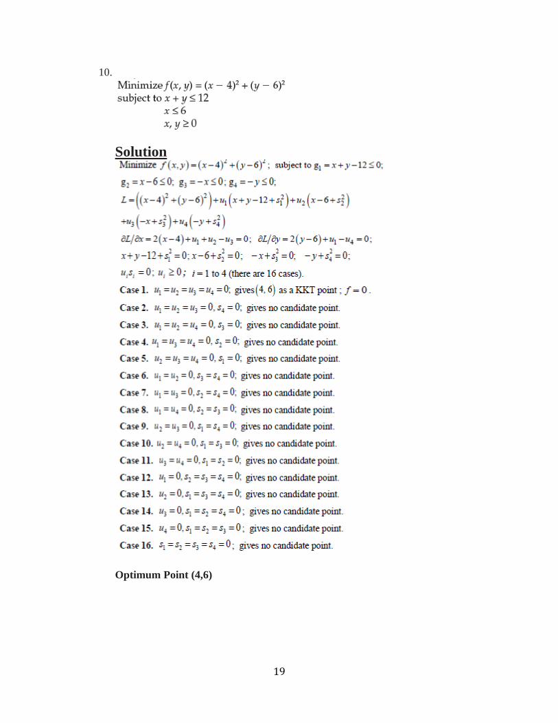
10.

Solution

Optimum Point (4,6)

20

21

MATLAB Code clear all

axis equal

[x,y]=meshgrid(-1:0.01:8, 2:0.01:10);

f=(x-4).^2+(y-6).^2;

g1=x+y-12;

g2=x-6;

g3=-x;

g4=-y;

cla reset

axis equal

axis ([-1 8 2 10])

xlabel('x'),ylabel('y')

title('Exercise 4.72')

hold on

cv1=[0:0.05:0.8];

const1=contour(x,y,g1,cv1,'g');

cv1=[0 0.01];

const1=contour(x,y,g1,cv1,'k');

cv2=[0:0.05:0.8];

const2=contour(x,y,g2,cv2,'g');

cv2=[0 0.01];

const2=contour(x,y,g2,cv2,'k');

cv3=[0:0.03:0.3];

const3=contour(x,y,g3,cv3,'g');

cv3=[0 0.005];

const3=contour(x,y,g3,cv3,'k');

cv4=[0:0.03:0.3];

const4=contour(x,y,g4,cv4,'g');

cv4=[0 0.005];

const4=contour(x,y,g4,cv4,'k');

fv=[0 1 4 9];

fs=contour(x,y,f,fv,'b');

a=[4];

b=[6];

plot(a,b,'.k');

grid

hold off

22

11.

Solution

23

Optimum Point (4,6)

24

MATLAB Code

clear all

axis equal

[x,y]=meshgrid(-4:0.01:12, -2:0.01:14);

f=(-1)*((x-4).^2+(y-6).^2);

g1=x+y-12;

g2=x-6;

g3=-x;

g4=-y;

cla reset

axis equal

axis ([-4 12 -2 14])

xlabel('x'),ylabel('y')

title('Exercise 4.74')

hold on

cv1=[0:0.05:0.8];

const1=contour(x,y,g1,cv1,'g');

cv1=[0 0.01];

const1=contour(x,y,g1,cv1,'k');

cv2=[0:0.05:0.8];

const2=contour(x,y,g2,cv2,'g');

cv2=[0 0.01];

const2=contour(x,y,g2,cv2,'k');

cv3=[0:0.03:0.3];

const3=contour(x,y,g3,cv3,'g');

cv3=[0 0.005];

const3=contour(x,y,g3,cv3,'k');

cv4=[0:0.03:0.3];

const4=contour(x,y,g4,cv4,'g');

cv4=[0 0.005];

const4=contour(x,y,g4,cv4,'k');

fv=[-52 -40 -36 -16 -4 -2 0];

fs=contour(x,y,f,fv,'b');

a=[4 6 0 6 5 0 6 0 6 4];

b=[6 0 6 6 7 0 0 12 6 0];

plot(a,b,'.k');

grid

hold off

25

12.

Solution

26

Optimum Point (3,2)

27

MATLAB Code

clear all

axis equal

[r,t]=meshgrid(-1:0.01:11, -1:0.01:8);

f=(-1)*((r-3).^2+(t-2).^2);

g1=r+t-10;

g2=t-5;

g3=-r;

g4=-t;

cla reset

axis equal

axis ([-1 11 -1 8])

xlabel('r'),ylabel('t')

title('Exercise 4.76')

hold on

cv1=[0:0.05:0.8];

const1=contour(r,t,g1,cv1,'g');

cv1=[0 0.01];

const1=contour(r,t,g1,cv1,'k');

cv2=[0:0.05:0.8];

const2=contour(r,t,g2,cv2,'g');

cv2=[0 0.01];

const2=contour(r,t,g2,cv2,'k');

cv3=[0:0.03:0.3];

const3=contour(r,t,g3,cv3,'g');

cv3=[0 0.005];

const3=contour(r,t,g3,cv3,'k');

cv4=[0:0.03:0.3];

const4=contour(r,t,g4,cv4,'g');

cv4=[0 0.005];

const4=contour(r,t,g4,cv4,'k');

fv=[0 -1 -4 -9 -12.5 -13 -18 -53];

fs=contour(r,t,f,fv,'b');

a=[3 3 0 3 5.5 0 0 10 5];

b=[2 0 2 5 4.5 0 5 0 5];

plot(a,b,'.k');

grid

hold off

28

13.

Solution

Optimum Point (60.5,1.008)