Munich Personal RePEc Archive Some Economics of Seasonal Gas Storage Chaton, Corinne and Creti, Anna and Villeneuve, Bertrand 21 July 2008 Online at https://mpra.ub.uni-muenchen.de/11984/ MPRA Paper No. 11984, posted 07 Dec 2008 15:27 UTC
Transcript
Munich Personal RePEc Archive
Some Economics of Seasonal Gas Storage
Chaton, Corinne and Creti, Anna and Villeneuve, Bertrand
21 July 2008
Online at https://mpra.ub.uni-muenchen.de/11984/
MPRA Paper No. 11984, posted 07 Dec 2008 15:27 UTC
Some Economics of Seasonal Gas Storage∗
Corinne Chaton† Anna Creti‡ Bertrand Villeneuve§
July 21th 2008
Abstract
We propose a model of seasonal gas markets which is flexibleenough to include supply and demand shocks while also consider-ing exhaustibility. The relative performances of alternative policiesbased on price caps and associated measures or tariffs are discussed.We illustrate with structural estimates on US data how this theorycan be used to give insights into the intertemporal incidence of policyinstruments.
1 Introduction
As energy markets become tenser and dependency on foreign imports in-crease in most economies, it is a challenging task to draw the picture of themodern gas industry. We analyze in a coherent framework this industry byfocusing on the economics of seasonal storage. Our approach is thus a use-ful complement to the models that focus on other relevant aspects of thegas industry, like transportation and its regulation (e.g. Teece, 1990, Banks,2007). We then broaden the scope by bringing into the picture gas priceshocks, trends as well as public policies.
Storage is the most natural source of flexibility in the gas sector, sinceconsumption, strongly influenced by weather, is seasonal and supply is rel-atively inflexible. Storing gas thus serves to avoid oversized extraction andtransportation infrastructures, as well as to limit excessive price fluctuations.
∗We are grateful to Jean-Christophe Poudou, Saıd Souam and Alban Thomas for theirvaluable remarks.
†Electricite de France R&D. E-mail: [email protected]‡Universita Bocconi and IEFE. E-mail: [email protected]§Universite de Tours, CREST (Paris) and Laboratoire de Finance des Marches
To focus on these economic mechanisms, we investigate the relationship be-tween stored quantities and prices in a model where time is discrete andinfinite. Years are split into two seasons, a simplification that is grosslyacceptable since we focus on aggregate dynamics of the economy. We char-acterize the competitive equilibrium and find realistic conditions for storageto be seasonal (stocks are empty each year at the end of winter). Stockpilingin summer and withdrawal in winter is shown to be consistent with randomshocks and exhaustibility of natural gas.
Although there would seem to be limited scope for government inter-vention in a competitive gas sector, public decisions are rarely motivatedby pure efficiency considerations. To clarify the effects of different policies,we characterize the best outcome a government can implement to maximizeconsumers’ surplus when gas is mainly imported. The basic novelty of ouranalysis is that, modeling seasonal storage, we explicitly take into account theintertemporal incidence of policy instruments such as a price cap associatedwith quantitative restraints, or taxes.
The price cap succeeds in smoothing prices but discourages storage andimplies winter rationing. We show that, in theory, this distortion can beattenuated by adopting side measures such as summer rationing. Taxes infact are a more effective policy instrument to exert monopsony power onforeign producers, as a multiseason scheme spreads the distortions betterthan a winter price cap. Taxes decrease consumption, domestic productionand imports compared to the competitive allocation. Whether storage isdiscouraged or not depends finely on the relative impact of taxes betweenthe two seasons.
We provide an illustration of our model by estimating and testing it onUS data. The US is the largest consumer of natural gas in the world (abouta quarter of the total) and also the largest importer (BP Statistical Review,2007).1 This market also offers an interesting perspective on policy inter-vention: according to the FERC Energy Policy Act of 2005, moderating therecurrence and severity of “boom and bust” cycles while meeting increasingdemand at reasonable prices is one of the major challenges facing the US nat-ural gas industry today. Rationing was common in the United States duringthe 1970s’ winters, as a consequence of restrictive regulatory policy on well-head prices. More recently, several examples of specific policy interventionscan be found at the state level in terms of excise taxes or gas price ceilingsas emergency measures.2 The estimation results show that the optimal price
1An overview of the US natural gas industry in Appendix A.1 recalls basic facts on theyearly gas cycle and gives orders of magnitude.
2Ohio levies a public utility excise tax on natural gas utilities and pipeline companies.Other States, like North Carolina, impose an excise tax on piped natural gas received for
2
cap is globally (i.e. in terms of social surplus) less distortionary than opti-mal tariffs, but it is less attractive for residents. The price cap discouragesstorage, as predicted, and more than tariffs.
The questions about storage are not new. In the theoretical literature, the“supply of storage” models (Kaldor, 1939, Working, 1948, Brennan, 1958)are mainly interested in the role of storage when the economy experiencesunexpected shocks. However, very few papers tackle the specific issues ofseasonal storage. Brennan (1960) sees it as a mere aspect of general purposemodels. Pyatt (1978) considers continuous time stationary demand and sup-ply subject to a fixed seasonal pattern that might not correspond. He showshow storage regulates the rate at which output increases over time. Lowryet al. (1987) analyze the role that storage plays in allocating supplies withinthe year in the soybean market. The authors characterize competitive spec-ulative storage and in particular estimate the expected price function usingcomputational rational expectations methods, when both demand and pro-duction are random.
Our focus on yearly cycles over an infinite horizon is a distinguishingfeature from storage models that use high frequency data for price simulationsand predictions in a short-medium term time frame (Urıa and Williams,2007).
A unique approach to some of the issues we address is to be found inAmundsen (1991), who investigates the social optimization problem of threeoperations: the extraction of natural gas from a reservoir up to its depletion,the supply to the storage unit (where either gas passes through or is stored),the transfer to end-users. Amundsen’s model is rich and complex. Dynamicsof extraction, inflows/outflows from storage, deliveries to consumers are con-nected so intricately that policy analysis is practically impossible. However,this issue is of crucial importance.
Public interventions through storage have taken several forms, as it canbe argued from different works. One set of models has analyzed the so-called“buffer stocks” that are used by public agencies to stabilize agricultural prices(Waugh, 1944, Oi, 1961, Massel, 1969). In these models storage costs and
final consumption. In emergency situations, gas price ceilings have been evoked, eventhough in practice these measures can be temporary or not implemented. This was thecase, for instance, in California, in 2001, when the Long Beach City Energy Director,considering that residential gas bills would likely have increased by about 34% comparedto the previous year, proposed a ceiling of $1 a therm (Bernstein et al., 2002). The decisionof the Aloha State to put into effect in August 2005 a new state law slapping a ceilingon gasoline prices pegged to average prices on the mainland, has raised a debate on thesurplus enhancing effect of price controls in the oil and gas industries (Committee onEnergy and Commerce, 2005).
3
management are simply abstracted away. Some trade models (for example,Hueth and Schmitz, 1972, Just et al., 1977, Devadoss, 1992) analyze publicmarket interventions that protect national interests from imported price fluc-tuations. Welfare gains are computed by comparing the economic situationwith and without stocks but storage is not optimized at the decentralizedlevel.
Williams and Wright (1991) have considerably enlarged the analysis ofstorage in dynamic stochastic models. Unfortunately, the complexity of theunderlying dynamic model makes the characterization of the effectiveness andefficiency of public interventions quite messy. Therefore, in the absence ofclear-cut explanations, only “rough” quantitative estimates of various welfareeffects of alternative government programs are computed numerically. Ourstylized model will simplify such evaluations.
In Section 2, we expose the main modeling assumptions. In Section 3,we characterize the competitive equilibrium under mild assumptions. Thebenchmark model opens the way to a detailed policy analysis in Section 4.We test the model using US data in Section 5. The estimates enable us toevaluate the impact on storage, prices and welfare of the policies we treatedtheoretically. The final section concludes. Proofs as well as estimates of thebasic model are relegated to the Appendices.
2 The model
The section sets up the model and characterizes the equilibrium.
Supply and demand. Six-month periods alternate between summer Sand winter W . A period is denoted by yσ with y for year and σ for season.The period that follows yσ is n(yσ) where n is for next; in particular n(yS) =yW and n(yW ) = (y + 1)S. We also use nm(yσ) and n−m(yσ), with m apositive integer, to indicate the mth period respectively after and before yσ.
The strictly decreasing consumption function at period yσ is denoted byConsyσ[·]. Production at period yσ is denoted by Prodyσ[·]. Production isnon-decreasing with respect to the price. We assume that for all periods yσ,consumption and production functions cross only once: the correspondingequilibrium price is denoted p0
yσ > 0. The difference between summer andwinter comes basically from the fact that the equilibrium summer price islower than the winter price. More precisely: p0
yW ≥ p0yS and p0
yW ≥ p0(y+1)S,
∀y. These natural conditions will directly make seasonal factors importantwithout assuming a purely cyclical repetition year after year.
4
Due to storage, prices are not determined by short term equilibria. Theprice in period yσ is denoted pyσ.
Competitive storage. Storage is assumed to be a competitive activitywith constant marginal cost c up to the maximum capacity K. The unitstorage charge in period yσ, denoted by κyσ, equals the marginal cost c if thecapacity constraint is slack, otherwise κyσ exceeds the marginal cost. Theinterest rate from one period to the next is r.
Total inventories Gyσ, counted at the end of yσ, cannot be negative. Ra-tional price-taking behavior leaves them null if there are no expected benefitsfrom storing. Those benefits come from capital gains (increase in unit priceof gas); costs are the direct rental price of storage (κyσ per unit) and theforegone interest (stored gas does not bear interest). This can be expressedas follows pn(yσ)
1 + r< pyσ + c ⇒ Gyσ = 0. (1)
An equivalent expression says that there are stocks only if prices follow aprecise evolution
Gyσ > 0 ⇒pn(yσ)
1 + r= pyσ + κyσ with κyσ ≥ c. (2)
To simplify the analysis, we summarize the response of the economy toprices by the aggregate excess supply function
△yσ[·] ≡ Prodyσ[·] − Consyσ[·]. (3)
For each period, conservation of matter imposes that the excess supply in oneperiod (positive or negative) is exactly equal to the stocks variation equation
△yσ[pyσ] = Gyσ − Gn−1(yσ). (4)
No bubble. We can easily argue that in any equilibrium with reasonablystable fundamentals, stocks have to revert to zero from time to time. A priori,with endogenous prices and storage, the equilibrium could be a “bubble” inwhich prices grow unboundedly after a certain period yσ, following the no-arbitrage equation (2)
pnm+1(yσ) = (1 + r) · (pnm(yσ) + κnm(yσ)), ∀m, with κnm(yσ) ≥ c. (5)
With this explosion of price, consumption shrinks and production grows pe-riod after period, implying ever increasing stocks, which is not credible. Toavoid the anomaly and retain only reasonable equilibria, it suffices to imposethat (5) is impossible.
5
Equilibrium. Absent storage, periods are not linked to each other econom-ically speaking. The equilibrium would be the unique sequence of prices p0
yσ
equalizing consumption and production every period (△yσ[p0yσ] = 0,∀y, σ).
But if in some period yσ, prices are such that
p0n(yσ)
1 + r> p0
yσ + κyσ, (6)
then storage creates value and is expected in equilibrium. This is typicallythe case if the price differential between successive prices is sufficiently high,the interest rate and storage costs are sufficiently low.
Definition 1 (Equilibrium) A competitive equilibrium starts in period 0S,with some stocks G0S; it is a sequence of gas prices pyσ, storage charges κyσ
and inventory levels Gyσ ≥ 0 such that, for all yσ after 0S
• ifpn(yσ)
1+r< pyσ + c then Gyσ = 0;
• ifpn(yσ)
1+r= pyσ + c then 0 ≤ Gyσ ≤ K;
• ifpn(yσ)
1+r= pyσ + κyσ with κyσ > c then Gyσ = K;
• △yσ[pyσ] = Gyσ − Gn−1(yσ);
• stocks go to zero every so often (no-bubble condition).
Price-taking behavior of the agents, strictly increasing excess supply func-tions, linearity of the storage technology, all these hypotheses suffice to ensurethat the competitive equilibrium maximizes the total surplus, obtained byadding consumers’ and producers’ surpluses each period discounted at theinterest rate. We retrieve the classical virtue of competition.
3 Seasonal storage
After the elimination of bubbles, it remains to be established that the equi-librium patterns are “simple”. This theoretical section shows that the alter-nation between stockpiling in summer and complete utilization of the stockin winter is a robust feature of the model.
6
3.1 Basic pattern
If the price is p in some period, N [p] ≡ (1+r)(p+c) denotes the price realizedthe subsequent period if storers decided to store. Consistently, Nm[p] denotesthe price attained after m seasons of uninterrupted stockholding.
The following condition restricts the rate at which supply and demand(thus excess supply) change over time. It says in particular that if a pricep cause additional stockholding, then the price attained after two seasonsof uninterrupted stockholding—that is N2(p)—is significantly higher than pand must cause additional stockholding two periods after.
Definition 2 The economy is said to be regular if for all seasons σ, all yearsy and all prices p
△(y+1)σ[N2[p]] ≥ △yσ[p]. (7)
If the economy’s fundamentals are purely cyclical (△yσ[·] does not changefrom year to year), then the above condition is satisfied.
The following proposition states that storage in regular economies is dom-inated by seasonal factors rather than by trends.
Proposition 1 (Seasonal pattern) If the economy is regular, then in anycompetitive equilibrium, storage becomes seasonal (stocks are empty each yearat the end of winter) after a finite number of periods and remains so.
Proof. See Appendix A.2.If the economy starts with huge reserves, prices start low and increase
steadily season after season following the no-arbitrage equation (2). Afterthe reserves have been exhausted once, which is inevitable given the no-bubble condition, the residual cycle would consist of stockpiling in summerand depleting reservoirs in winter.
The seasonal cycle means that years are independent of each other. Thissimplification enables us to characterize the equilibrium for any year y. As-sume a large K to ensure that κyS = c. There are two cases. If p0
yW /(1+r) ≤p0
yS + c and there are no inventories, for lack of profitability. If p0yW /(1+r) >
p0yS + c, the two prices (pyS, pyW ) are determined by two fundamental equa-
tions: conservation of matter (equation 4), and no-arbitrage condition (equa-tion 2). Storage smooths prices: the summer price increases and the winterprice decreases but remains higher. Consequences on consumptions are di-rect: an decrease in summer and an increase in winter.
Figure 1 illustrates the case of the two-season equilibrium with lineardemand, a production function independent of the season (the year index isdropped), and sufficient storage capacity K.3
7
✻
✲�
��
��
��
��
��
��
��
��
��
��
❏❏
❏❏
❏❏
❏❏
❏❏
❏❏❏
❏❏
❏❏
❏❏
❏❏
❏❏
❏❏❏
Cons, Prod
p ConsW Prod
ConsS
pS
G︷ ︸︸ ︷
︸ ︷︷ ︸G
pW
p0W
s s
p0S
s s
ConsS ProdS ProdW ConsW
Figure 1: Unconstrained Competitive Storage.
3.2 Shocks
The property that stocks are fully used at the end of the winter is gener-alizable to a stochastic version of the model. Assume that season specificshocks impact the excess supply function (i.e., fundamentally, supply anddemand) and that this shock is known only at the beginning of the season.This means simply that decisions made one season before were not informedof the magnitude of the upcoming shock, whereas decisions taken during theseason take it into account. Temperature and weather conditions in generalare good examples.
The heuristic is the following. Take a deterministic economy as studied inthe previous paragraphs and assume conditions are met for a cyclical pattern.If we perturb the model by adding “small” shocks then there is no possiblestate of the economy in which speculators store at the end of the winter forthe coming summer. The question is to define “small”.
The first step to show that this approach works is to solve the equilibrium
3Remark that if K is saturated at the end of the summer, we have one more unknown(κyS instead of c), and one more equation (GyS = K), which leaves the system solvable.The endogenous storage charge generates a scarcity rent κyS − c.
8
by treating each year separately assuming that each year starts and finisheswith empty stocks. This amounts to reasoning as if interyear storage wereforbidden. The resulting equilibrium prices are random: the summer pricedepends on the summer shock (plus expectations as for the winter shock tocome), the winter price depends on the summer (through the past storagedecisions) and winter shocks. This generates the supports for summer andwinter prices. The second step is to search for conditions under which storagefrom winter to summer is never desirable in any realization of the possiblestates of nature. It suffices to compare the smallest possible winter pricewith the expected subsequent summer price. If the former is high enough(or equivalently, if the latter is low enough), then storage is never profitable.This implies that stockout at the end of winters is systematic. The conditionto obtain this result is to have shocks of limited magnitude (with respect tothe no-storage price range) in both summer and winter.
3.3 Trends and cycles with exhaustible reserves
Natural gas is an exhaustible resource: the equilibrium cannot be stationary,except if production and consumption become null. We examine now the im-plication of this property for a “seasonal” model. We show that the economycrosses three significantly different phases. The intermediate one, which maybe very long, exhibits interesting and empirically important cyclical features.
3.3.1 A simple model
We assume that finite gas reserves are concentrated at a unique wellhead H.Consumption is concentrated in a unique region B (Burnertips). A pipelineof capacity Q (per period) connects H and B. Marginal extraction cost iscH, while marginal transportation cost along the pipeline is cT (both cH andcT are assumed to be constant and stationary).4 Storages are located at B.Each period, gas can either be kept in the original field (i.e. not produced)or stored in the consumption region once it has been transported there. Thedifference between the gas field and storages lies in stockholding costs (zeroin the former and c per unit per period in the latter). See Figure 2 for asimple illustration.
We assume that all agents are price-takers and that all arbitrage possi-bilities (through transportation or storage) are exploited. The price at nodei (= H, B) and period yσ is denoted by pi
yσ. The unit profit at H for period
4Remark that Q could alternatively be interpreted as the maximum capacity of theproduction sector.
9
Figure 2: Extraction, storage, burning.
yσ is pHyσ − cH, which, according to the Hotelling rule, grows at rate r. This
impliespH
n(yσ)
1 + r− pH
yσ = −r
1 + rcH < 0. (8)
The wellhead price grows more slowly than the interest rate.We consider an economy in which gas demand functions in winter and
summer are stationary. Inverse demand functions in summer S and andwinter W are denoted by pS[·] and pW [·] respectively. To keep the economi-cally appealing case in which seasonal storage is desirable when imports aremaximum (line is congested), we assume that pW [Q]/(1 + r) > pS[Q] + c.
To simplify matters, we assume that, during the first period, stocks areempty (no domestic gas fields). We describe the situation at “the beginning”(low prices), during the transition (intermediate prices) and at “the end”(high prices). A more realistic description would be a model in which fieldsare increasingly costly or increasingly remote from the consumption region asdepletion goes on. The effects for consumers would remain roughly identicalwith similar phases.
3.3.2 Three phases
Large reserves/Low prices. Demand is high and the pipeline is fullyused in both seasons. In the absence of storage, prices would be pB
yS = pS[Q]and pB
yW = pW [Q]. The assumption above on these prices ensures that there is
some storage G taking place, the unique solution to the following no-arbitrageequation
pW [Q + G]/(1 + r) = pS[Q − G] + c. (9)
The equilibrium prices are pByS = pS[Q − G] and pB
yW = pW [Q + G].The economy follows a trend at H, but is strictly cyclical at B (seasonal
consumer prices and quantities consumed or stored are constant). The total
profits (mineral rent plus pipeline congestion rent) are (pS[Q−G]−cH−cT)Q
10
in summer and (pW [Q + G] − cH − cT)Q in winter. Remark also that thisglobally constant rent is gradually transferred from the pipeline owners tothe reserve owners; indeed, pB
yσ increases over the years, whereas pHyσ is sta-
ble. Over time, the transportation network becomes less and less profitable.Storage is competitive and thus produces no net profit.
Intermediate reserves/Intermediate prices. The line is congested inone season only.
If the pipeline is fully used in winter only, the assumption according towhich pW [Q]/(1 + r) + c > pS[Q] ensures that some storage will take place.The price in summer is the wellhead price plus transportation charge cT andthe price in winter is driven by the no-arbitrage condition
pByS = pH
yS + cT, (10)
pByW = (1 + r)(pB
yS + c). (11)
This is the normal and realistic situation.In the case where congestion occurs in summer only, we have
pByS > pH
yS + cT, (12)
pByW = pH
yW + cT. (13)
By rearranging these two equations, we find
pByW
1 + r− pB
yS < −r
1 + r(cH + cT). (14)
This precludes storage (the RHS is obviously smaller than c). Congestion insummer always goes with no storage; this case is therefore quite unrealisticbut it cannot be logically excluded without making further assumptions ondemand functions.
Low reserves/High prices. The line becomes uncongested in both peri-ods and necessarily pB
yσ = pHyσ + cT for each period, i.e.
pBn(yσ)
1 + r− pB
yσ = −r
1 + r(cH + cT) < 0 < c. (15)
Prices grow more slowly at B than at H, a fortiori more slowly than theinterest rate. This eliminates any incentive for storage and the consumersrely entirely on current imports. Remark that the mineral rent remains nowintegrally in the hands of the producers.
11
The first phase is specially relevant for economies that depend highly onenergy imports. Price observed at the local level may well be stationary fora while, even if the world price follows the Hotelling rule. An interestingfeature of the second phase is diminishing reliance on storage and dissipationof the pipeline rent.
4 Policy analysis
The independence between years guaranteed by Proposition 1 can be ex-ploited to analyze policy within years. Consequently, the year index y willbe dropped in the following to make for easier reading. After analyzing basicprice caps, we characterize the best outcome a government can implement tomaximize consumers’ surplus as well as the instruments that can be used.
4.1 Price cap
A price cap only forces prices not to exceed a certain value, denoted byp. Markets are otherwise competitive: economic agents take prices as given,therefore the cap could generate a disequilibrium between supply (productionand release from inventories) and demand (consumption).
If p is higher than the winter price pW expected in the absence of a ceiling,then it has no effect on the economy. If it is too low, it completely discour-ages storage since the price dynamics motivating stockpiling in summer issterilized; this happens if p ≤ (1 + r) · (p0
S + c).For intermediate values ((1 + r) · (p0
S + c) < p < pW ), we have theeconomically interesting case where winter demand is larger than supply.We assume in that case that consumption is rationed efficiently (consumerswith higher valuations are served first), which simplifies the calculation ofthe surplus. In equilibrium, prices and stocks are denoted, respectively, bypS, pW and G to show their dependency on the price cap p.
Proposition 2 For economically relevant price caps, i.e. (1+ r) · (p0S + c) <
Proof. See Appendix A.3.Though price ceilings succeed in reducing prices, price variability remains
little affected and storage is discouraged. The latter effect was mentioned in,e.g., MacAvoy and Pindyck (1973) and Wright and Williams (1982b).
If the government in charge of setting the price cap defends the consumers’interest only, then a price cap is desirable.5 There are obvious limits tothese gains: the deadweight loss is approximately quadratic with respect tothe difference between the price cap and the free price, while the price capgenerates an approximately linear transfer in favor of the consumers.
As price caps are a way of exerting market power, the result is in line withmonopsony pricing theory (here the state “coordinates” consumers throughthe ceiling), with intertemporal effects due to competitive storage. The prac-tical difficulty is not to go too far once the cycle is fully taken into account.An improvement is to combine the price cap and the inevitable winter ra-tioning with some summer rationing. As the rationing cost is approximatelyquadratic with respect to the difference between demand and supply, rebal-ancing rationing between seasons enhances welfare. This raises the issue of
5Symmetrically to the discouragement effect of the price cap, a price floor higher thanthe undistorted one will create excess storage and therefore will sacrifice economic effi-ciency (Helmberger and Weaver, 1977). Producers gain from the government policy, whileconsumers lose.
13
finding the optimal policy.
4.2 Optimal price policy
To optimize the consumers’ or the domestic surplus, we need to be morespecific as to fundamentals. The simplest approach is to represent consumerswith an intertemporal utility function; the arguments are gas consumptionand a separable numeraire that could be seen as labor. The consumers yearlysurplus can then be written
US[qCS ] − mS +
UW [qCW ] − mW
1 + r, (16)
where US and UW are increasing and concave utility functions, qCσ is season
σ gas consumption and mσ is season σ expenditure. The year index y isdropped without loss of generality. Domestic production is simply modeledthrough cost functions CD
S [·] and CDW [·]; imports are represented with the
inverse supply functions pIS[·] and pI
W [·] respectively. Storage is assumed tobe domestic.
The optimal policy in the interest of the residents (consumers plus domes-tic producers) can be characterized using the following method: all quantities(qC
S and qCW , domestic productions qD
S and qDW , and imports qI
S and qIW ) are
taken as choice variables. Domestic production is accounted for its cost whileimports are accounted for the expenditure. The stocks are qD
S + qIS − qC
S . Thegovernment solves
maxqCS
,qCW
,qDS
,qDW
,qIS
,qIW
US[qCS ] − CS[qD
S ] − pIS[qI
S]qIS
+UW [qC
W ]
1 + r−
CW [qDW ]
1 + r−
pIW [qI
W ]qIW
1 + r−c(qD
S + qIS − qC
S )
such that qDS + qI
S + qDW + qI
W ≥ qCS + qC
W ,qDS + qI
S ≥ qCS .
The first constraint states that total consumption must not exceed totalproduction and imports. The second one states that stocks are positive.
We only discuss the case of strictly positive storage at the end of thesummer (the last constraint is slack). The necessary and sufficient conditions,
14
after elimination of the Lagrange multipliers, are
U ′
S[qCS ] = C ′
S[qDS ], (17)
U ′
W [qCW ] = C ′
W [qDW ], (18)
U ′
S[qCS ] + c =
U ′
W [qCW ]
1 + r, (19)
U ′
S[qCS ] = pI
S[qIS] + pI′
S [qIS] · qI
S, (20)
U ′
W [qCW ] = pI
W [qIS] + pI′
W [qIW ] · qI
W , (21)
qDS + qI
S + qDW + qI
W = qCS + qC
W . (22)
The interpretation of the first three equations straightforward: equations(17) and (18) only require that consumers’ marginal utilities equal domesticmarginal costs; (19) consumers’ intertemporal MRS should satisfy the no-arbitrage equation (domestic storage must not be distorted). Equations (20)and (21) show how the government should exert its monopsony power onforeign producers.
Proposition 3 Compared to the competitive allocation, the best allocationfor consumers is such that consumptions, domestic productions and importsat each period decrease. The benefits come from lower import prices eachperiod.
Proof. See Appendix A.4.Storage may be greater with the optimal policy than under laissez-faire.
This possibility was existent with the less efficient price cap policy. Assumefor example that winter demand is very inelastic compared to summer de-mand. Since production is reduced in both periods, winter demand can bemet only by discouraging summer demand. Given the elasticities, this is theless distortionary choice; accordingly, one has to increase the stored quantityof gas.
4.3 Implementation
The allocation maximizing domestic surplus can be sustained with tariffson imports each season (denoted by τS and τW ) and competitive markets.No intervention is required in the domestic market (storage sector included):consumption is not rationed and domestic storers simply arbitrage. Each sea-son, the import price plus the tariff equals the domestic price. The domesticprices are simply denoted pS and pW .
This gives:
15
Domestic prices: pS = U ′
S[qCS ] = C ′
S[qDS ],
pW = U ′
W [qCW ] = C ′
W [qDW ].
Import prices: pIS = pI
S[qIS],
pIW = pI
W [qIW ].
Tariffs: τS = pI′S [qI
S]qIS > 0,
τW = pI′W [qI
W ]qIW > 0.
The interpretation of price policy in terms of taxation unifies the viewon the various policies that have been or could be observed or proposed. Wedisagree with Wright and Williams (1982b) who write that “a price ceiling cancrudely substitute for an optimal tariff, if this latter cannot be implemented.”Indeed, a price cap supposes controls and rationing, as we saw earlier; butefficient rationing is extremely demanding in terms of information becauseit requires knowledge of the private marginal valuations of all the consumerswhereas the tariff merely requires uniform application. The government canimplement the same allocation just by imposing a well calculated tax.6
Above all, optimal tariffs implement an optimally balanced “rationing”(or preferably demand containment) between summer and winter, whereasthe version we discussed in 4.1 concentrates the effort on winter, which issuboptimal. Moreover, as it is typical of second best policy, this primarydistortion must be mitigated by other distortions. The government may wishto compensate the undesirable effects of the basic price cap (discouragingstorage) with subsidies on storage (or, if one prefers, subsidies across periods).Tariffs are simpler.
5 Applications
The liberalization of the US gas market is now sufficiently well established(Hirschhausen, 2007) to provide data on prices and quantities that can beused to estimate structural parameters and test a number of our model’spredictions (Appendix A.5). Though the results are satisfactory in manyways, the accuracy of the estimates drawn from the aggregate approach isinsufficient to formulate firm predictions. With this reservation in mind,
6Wright and Williams (1982b) assumed that consumption is rationed by marketablecoupons distributed to consumers. Therefore, a kind of “secondary spot markets” mustexist for rationing to be efficient (the least costly in terms of welfare). This idea goesagainst the principle of a price cap, since some transactions are indeed made above theceiling. In all events, such markets seem to be quite unlikely to emerge at the finalconsumption level.
16
we propose a comparative simulation of the impact of various price policiesdiscussed in Section 4.
Evaluation of the welfare effects of price policies. To focus on pricepolicies, we reason on the average year (sample average temperature, GDP,number of wells). Linear demand and supply functions are integrated to givelinear-quadratic utility and cost functions. We compare three scenarios usingthe structural parameters estimated under the assumption that markets arecompetitive:
1. Pure competition.
2. The optimal price cap for residents (consumers and domestic producers)with winter efficient rationing (see Subsection 4.1).
3. The residents’ optimum: tariffs only, no rationing (see Subsection 4.2).We calculate optimal τS and and associated equilibrium prices andquantities (see Subsection 4.3).
We start by estimating directly the structural equations of the modelunder a linear specification using the 3SLS. For each year, the equilibriuminvolves four equations: excess supplies in summer and in winter, price ar-bitrage and annual balance. The observed variables for season yσ are thevariation of the stock, the average gas price, GDP and average temperature.Appendix A.5 describes our procedure and results. The tests of theory basedlinear restrictions and signs are passed.
The four core equations only require stock variations. To evaluate welfare,we must complement them with some structural estimates of demand andsupply. In principle estimating precisely demand and supply would require amore comprehensive dynamic theory and this route would be very demandingin terms of data. We have limited ourselves to a very summary model. Thisgives us a first complete set of parameters to perform comparisons such asthose exposed in Table 1. See Appendix A.6.
The total maximum surplus is set by convention to 0 in Table 1;7 othersurpluses are given as differences with the maximum. The optimal price capis overall less distortionary than optimal tariffs; the latter are nevertheless,by definition, more attractive for residents. The optimal tariffs are very large(about $7 per MMcf) and do more than halve the import price. This effect isdue to the relative inflexibility of imports. The price cap discourages storage,as predicted, and more than tariffs, whose effect is ambiguous in theory.
7The value found by integration of the demand and supply functions is B$ 6.21. How-ever this calculation involves extrapolating the functions well beyond the sample.
17
Scenario Perfect comp. Opt. price cap Opt. tariffs
Total surp./year 0.00 −1.06 −1.84Dom. surp./year −12.70 −11.50 −10.40
Quantities in MMcf, prices in $/MMcf, surpluses in M$.
A limit to this exercise is that, in accordance with the estimation results,the optimal policy should be conditional on observables like temperatureor GDP. More importantly, though the elasticity of imports seems low andthus “justifies” high tariffs, in the long run elasticity, through investment byproducers to deliver gas towards more profitable regions, is certainly muchgreater. The extent of US market power over external providers is also hardto measure. Obviously, the NAFTA prevents any such attempts towardsCanadian imports, which nevertheless leaves some leeway for other imports.In any case, the modest extra surplus calculated (in absolute value) could beseen to be upper bounds of the potential benefits.8
6 Conclusion
The model enabled us to expose a comprehensive view of seasonal naturalgas markets. Economies are neither stationary nor purely cyclical. One ofour insights is the description of a yearly pattern which is preserved oneconsiders moderate shocks and the exhaustibility of this natural resource.This flexibility enables us to directly formulate our theory in a 4-equationstructural model. The estimates based on the US data over 1986-2005 areconsistent with a number of theoretical restrictions. The potential surplusgains that the country could achieve are calculated.
8The interplay between tariffs and price cap was addressed by Wright and Williams(1982), who analyze public policies as a response to an oil supply disruption due to ran-dom shocks. However, in the Wright-Williams model, the relative effects of the two pricepolicies, namely the price cap and the import tariffs, are difficult to disentangle as embed-ded in a very complex dynamic game, with government and the private sector interactingstrategically.
18
Our analysis can be used as a building block of a model where one con-siders regulatory issues such as access to storage or transportation charges.If the storage capacity is saturated at the end of the summer, the endoge-nous storage charge generates a scarcity rent. Under competition, allowingusage rights with regulated storage prices or leaving prices unregulated onlychanges the allocation of the rent, since the prices and quantities exchangedand stored are unaffected. The rent is simply left to those who detain theright to store. Both usage rights with regulated storage prices and unreg-ulated prices lead to the social optimum in which the scarcity rent is themarginal welfare loss due to the constraint. This equivalence is only truein the short run; in the long run investment becomes a serious issue. Forregulators, the balance between preserving incentives to invest (rents) andfighting market power requires information on the long run marginal cost,whose evaluation is enormously complicated by the huge heterogeneity ofpossible sites (location, geological characteristics). Though rents are not perse proofs of noncompetitive behavior, the regulator must be able to distin-guish a case of true scarcity from an abuse of market power via voluntaryrestriction of supply. In this respect, the caution of FERC in allowing gascompanies to use market-based rates for storage access instead of regulatedtariffs, is understandable.9
References
[1] Amundsen, Erik Schroder (1991): “Seasonal Fluctuations of Demand and Optimal
Inventories of a Non-renewable Resource Such as Natural Gas,” Resources and En-
ergy, 13, 285–306.
[2] Banks, Ferdinand E. (2007): “The Political Economy of World Energy: An Intro-
ductory Textbook,” World Scientific.
[3] Balestra, Pietro and Marc Nerlove (1966): “Pooling Cross Section and Time Se-
ries Data in the Estimation of a Dynamic Model: The Demand for Natural Gas,”
Econometrica, 34, 585–612.
9FERC Order 636 opens access to gas storage at regulated prices that comprise a fixedcapacity charge (reservation or booking fee) and a commodity charge (according to us-age). Market-based tariffs can be applied where sufficient competition between facilities isdemonstrated. To obtain market-based prices, large pipeline companies have to argue thatindustry restructuring and network interconnections have effectively broadened the mar-ket for storage beyond some narrow geographic area where that company predominates,and that prospective storage customers actually have many good alternatives.
19
[4] Bernstein, Mark, Paul Holtberg and David Santana-Ortiz (2002): “Implications and
Policy Options of California’s Reliance on Natural Gas,” RAND Monograph Report,
available at http://www.rand.org.
[5] Brennan, Michael J. (1958): “The Supply of Storage,” American Economic Review,
48, 50-72.
[6] Brennan, Michael J. (1960): “A note on Seasonal Inventories: Reply,” Econometrica,
28, 921-922.
[7] BP Statistical Review (2007), available at http://www.bp.com.
[8] Committee on Energy and Commerce (2005): Hearing to Examine Hur-
ricane Katrina’s Impact on U.S. Energy Supply, available at energy-
commerce.house.gov/108/Hearings.
[9] Devadoss, Steven (1992): “Market Interventions, International Price Stabilization,
and Welfare Implications,” American Journal of Agricultural Economics, 74, 281–
290.
[10] EIA (2006): “U.S. Underground Natural Gas Storage Developments: 1998-2005.”
[11] Helmberger, Peter and Rob Weaver (1977): “Welfare Implications of Commodity
Storage under Uncertainty,” American Journal of Agricultural Economics, 59, 639–
651.
[12] Hirschhausen, Christian von (2008): “Infrastructure, Regulation, Investment and
Security of Supply: A Case Study of the Restructured US Natural Gas Market,”
Utilities Policy, 16, 1-10.
[13] Hotelling, Harold (1931): “The Economics of Exhaustible Resources,” Journal of
Political Economy, 39, 137–175.
[14] Hueth, Darrell and Andrew Schmitz (1972): “International Trade and Final Goods:
Some Welfare Implications of Destabilized Prices,” Quarterly Journal of Economics,
86, 351–365.
[15] Just, Richard E., Ernst Lutz, Andrew Schmitz and Stephen Turnovsky (1977): “The
Distribution of Welfare gains from International Price Stabilization under Distor-
tions,” American Journal of Agricultural Economics, 59, 652–661.
[16] Kaldor, Nicholas (1939): “Speculation and Economic Activity,” Review of Economic
Studies, 7, 1-27.
20
[17] Lowry, Mark, Joseph Glauber, Mario Miranda and Peter Helmberger (1987): “Pric-
ing and Storage of Field Crops: A Quarterly Model Applied to Soybeans,” American
Journal of Agricultural Economics, 9, 740-749.
[18] MacAvoy, Paul W. and Robert S. Pindyck (1973): “Alternative regulatory Policies
for Dealing with the Natural Gas Shortage,” Bell Journal of Economics and Man-
agement Science, 4, 454–498.
[19] Massel, Benton F. (1961): “Price Stabilization and Welfare,” Quarterly Journal of
dictive Performance, and the Theory of Storage,” Energy Economics, 27, 617–637.
[21] Oi, Walter (1961): “The Desirability of Price Instability Under Perfect Competition,”
Econometrica, 29, 58–64.
[22] Pyatt, Graham (1978) “Marginal Costs, Prices and Storage,” Economic Journal, 88,
749-762.
[23] Urıa, Rocıo and Jeffrey Williams (2007): “The Supply of Storage for Natural Gas in
California,” The Energy Journal, 28, 31–50.
[24] Teece, David J. (1990): “Structure and organization in the Natural Gas Industry,”
The Energy Journal, 11, 1–35.
[25] Waugh, Frederic V. (1944): “Does the Consumer Benefit from price Instability?,”
Quarterly Journal of Economics, 53, 602–614.
[26] Williams, Jeffrey C. and Brian D. Wright (1991): Storage and Commodity Markets,
Cambridge University Press.
[27] Wilson, Robert (1989): “Efficient and Competitive Rationing,” Econometrica, 57,
1–40.
[28] Working, Holbrook (1948): “Theory of the Inverse Carrying Charge in Futures Mar-
kets,” Journal of Farm Economics, 30, 1–28.
[29] Wright, Brian D. and Jeffrey C. Williams (1982): “The Roles of Public and Private
Storage in Managing Oil Import Disruptions,” Bell Journal of Economics, 13, 341–
353.
21
A Appendices
A.1 The US gas cycle
Weather is the primary driver of gas consumption. Because of winter heating,the seasonal pattern of gas deliveries is particularly striking in the residentialand commercial sectors. Due to power-generation demand for summer cool-ing, the electric utilities’ consumption is counter-cyclical (3.4 times higherin July and August than in January and February). Nevertheless, the over-all seasonal pattern is not offset: the yearly cycle alternates between winterpeaks and summer troughs. This is illustrated in Figure 4.
In contrast, extraction from gas wells as well as imports are practicallyflat (see Figure 5). A smooth production is motivated by cost-efficiency ar-guments driven by geological considerations.10 In addition, production andtransportation are highly capitalistic and complementary; the economic opti-mum requires maximum utilization of the infrastructure and the profitabilityof the investment is typically secured by long term contracts with limited flex-ibility. Imports into the United States—almost entirely from Canada—showslightly more of a seasonal pattern than US production, largely because of theextensive use of Canadian upstream storage. The US gas industry is highlydiversified with no single dominant company. According to the Natural gasAssociation, there are about 8,000 gas producers, ranging from small opera-tions to major international oil companies. The five largest producers (BP,ExxonMobil, Chevron-Unocal, Devon Energy, ConocoPhillips, ChesapeakeEnergy) account for around 25% of total US output.
Storage plays a key role in balancing seasonal and short-term loads (com-pare total consumption in Figure 4 with net withdrawals in Figure 5). Nat-ural gas, unlike many other commodities, requires specialized facilities. Thereare several types of storage: depleted gas or oil fields, aquifers, salt caverns,liquefied natural gas (LNG) tanks. Pipelines can also be used for balancingthe transmission flows in order to keep gas pressure within design parame-ters. Each type has its own economic and physical characteristics. In general,storage facilities are classified according to flexibility (high or low withdrawaland injection rates). The two main classes are high deliverability sites (saltcavern reservoirs and LNG storages) and seasonal supply reservoirs (depletedfields and aquifers). Most existing gas storage in the United States is in de-pleted natural gas or oil fields that are close to consumption centers. Seasonalsupply reservoirs are usually drawn down during the heating season (about150 days from November to March) and filled during the non-heating season
10For example, excess withdrawal of gas can submerge the wells with liquids (water,oil), causing interruption of the gas flow.
22
0
0,5
1
1,5
2
2,5
01-0
1
03-0
1
05-0
1
07-0
1
09-0
1
11-0
1
01-0
2
03-0
2
05-0
2
07-0
2
09-0
2
11-0
2
01-0
3
03-0
3
05-0
3
07-0
3
09-0
3
11-0
3
01-0
4
03-0
4
05-0
4
07-0
4
09-0
4
11-0
4
01-0
5
03-0
5
05-0
5
07-0
5
Total consumption
Residential consumption
Industrial consumption
Commercial consumption
Electric utilities
Figure 4: Gas consumption (total and by end use) (Tcf). Source: EIA.
-0,5
0
0,5
1
1,5
2
01-0
1
03-0
1
05-0
1
07-0
1
09-0
1
11-0
1
01-0
2
03-0
2
05-0
2
07-0
2
09-0
2
11-0
2
01-0
3
03-0
3
05-0
3
07-0
3
09-0
3
11-0
3
01-0
4
03-0
4
05-0
4
07-0
4
09-0
4
11-0
4
01-0
5
03-0
5
05-0
5
07-0
5
Production
Domestic production
Imports
Exports
Storage net withdrawals
Figure 5: Withdrawals from gas wells and imports (Tcf). Source: EIA.
23
(about 210 days from April through October). High deliverability sites canbe rapidly drawn down (in 20 days or less) and refilled (in 40 days or less) inorder to respond to less expectable peak demands or system load balancing.
In 2005, the US industry had the capability to store approximately 8.2trillion cubic feet (Tcf) of natural gas in about 391 storage sites around thecountry, mostly in depleted gas or oil fields. Working gas capacity makes upslightly less than 50% of the total. The rest goes to the base (or cushion)gas, i.e. the permanent volume of gas in a storage reservoir necessary tomaintain adequate pressure and deliverability rates during the withdrawalseason. In 2005, the gas withdrawn from storage to end use was 3.047 Tcf,which represents 13.2% of total gas supplies.
At the close of 2005, 394 underground natural gas storage facilities wereoperational in the US although 37 were marginal operations that reportedlittle or no activity during the year. Between 1998 and 2005, 42 facilities wereabandoned as uneconomic or defective, representing a loss of 223 billion cubicfeet (Bcf) in total capacity, while 26 new sites, accounting for 212 Bcf of newcapacity, were placed in operation. Yet, as abandoned capacity was alwayscompensated for with new storage field development and the completionof several storage expansion projects, working gas capacity and design-daywithdrawal capability (deliverability), the two prime measures of storageutility in today’s natural gas storage market, grew steadily and substantially.By 2008, more than 73 underground natural gas storage projects are expectedto be undertaken: they have the potential to add as much as 0.346 Tcf toexisting working gas capacity (EIA, 2006). New storage sites are mainly saltcaverns.
In recent years, the price of natural gas has followed an upward slope toreach unprecedented levels. The development of new production capacity islagging behind growth in demand, which is also exacerbated by the use ofgas for electric power production. Because of the existence of a significantamount of short-term fuel-switching capability in industry and power gen-eration, interfuel competition plays a major role in day-to-day price setting.This demand-side flexibility limits the seasonal volatility of spot prices: inthe Northeast and Mid-Atlantic, prices are effectively capped by prevailingheavy-fuel-oil price levels in the winter, when oil typically replaces gas inpower generation and in some industrial uses. The ability of power genera-tors to burn coal in the South effectively sets a ceiling price for gas in thesummer. The sustained tension on the market results in large spikes whenthe temperature reaches unusually low levels in winter or unusually high lev-els in summer. Accidents like the breakdown in 2001 of the El Paso pipelineconnecting California to Mexico or natural disasters like Hurricane Katrinain 2005 had similar effects. In 2006, the prices have returned to levels closer
24
0
1
2
3
4
5
6
7
8
9
10
01-0
0
03-0
0
05-0
0
07-0
0
09-0
0
11-0
0
01-0
1
03-0
1
05-0
1
07-0
1
09-0
1
11-0
1
01-0
2
03-0
2
05-0
2
07-0
2
09-0
2
11-0
2
01-0
3
03-0
3
05-0
3
07-0
3
09-0
3
11-0
3
01-0
4
03-0
4
05-0
4
07-0
4
09-0
4
11-0
4
01-0
5
03-0
5
05-0
5
07-0
5
City gate price
Wellhead price
Figure 6: Monthly natural gas price ($/Mcf). Source: EIA.
to historical average.In this context, in contrast to previous decades, the seasonality of the
price is hardly visible in Figure 6. However, over the last twenty years, theaverage price over the winter is significantly higher than the average priceduring the previous summer.
A.2 Proof of Proposition 1
The no-bubble condition imposes that the stocks become necessarily nullin finite time. We show by contradiction that from then on, stockholdingremains seasonal (holding stock two or more successive periods is impossible).
Suppose that there is an integer m ≥ 3 such that stocks are null at theend of yσ, strictly positive at the end of the periods nj(yσ) for 1 ≤ j < m,and null at the end of nm(yσ). The stock at the end of period nj(yσ) forj ≤ m is
Gnj(yσ) =
j∑
i=1
∆ni(yσ)[Ni[pyσ]], (23)
Given that the economy is regular (see definition 2), for all j such that
25
3 ≤ j ≤ m
Gnj(yσ) − Gn2(yσ) =
j∑
i=3
∆ni(yσ)[Ni[pyσ]] >
j−2∑
i=1
∆ni(yσ)[Ni[pyσ]] = Gnj−2(yσ).
(24)This equation displays a contradiction for j = m : the LHS is negative, whilethe RHS is positive.
A.3 Proof of Proposition 2
1. The parallel evolution of the two prices pS and pW is due to the no-arbitrage equation ( pW
1+r= pS + c) satisfied whenever storage is positive, and
to the fact that the constraint binds during peaks: pW = p. To see that stor-age is discouraged, observe that demand during summer increases whereasproduction decreases (as current price is decreased). This immediately im-plies that in winter demand exceeds supply and consumers are rationed.
2. We start from the unconstrained competitive equilibrium. Let uschoose p = pW − dp, with small dp > 0. We get pW = p and pS = pS − dp
1+r.
The impact on the consumer’s surplus during summer is positive and offirst order with respect to dp since they only benefit from the lower price.During winter, on the one hand they benefit from lower prices (first-ordereffect), but on the other hand, demand is increased (first-order) while supplyis decreased (negative first-order effects on production and storage). Thisrationing only provokes second-order effects on winter surplus, therefore thebenefits dominate the loss for small dp.
A.4 Proof of Proposition 3
Equation (19) holds in the competitive and the monopsony allocations, im-plying that qC
S and qCW are both higher or lower in the latter. We show by
contradiction that they are lower. Assume that qCS and qC
W are higher. TheLHS of equations (20) and (21) decrease, meaning that qI
S and qIW decrease.
Similarly, equations (17) and (18) imply that qDS and qD
W also decrease. Thiscontradicts equation (22).
Remark that G = qDS + qI
S − qCS . Depending on which of production and
consumption in summer is most impacted by the government policy, G in-creases or decreases with respect to the competitive benchmark. One caneasily verify with a linear version of the model that both cases are possible.
26
A.5 Estimation of the model
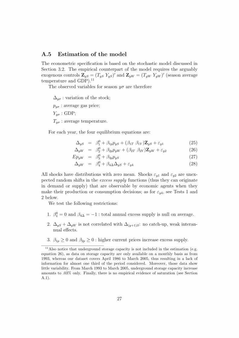
The econometric specification is based on the stochastic model discussed inSection 3.2. The empirical counterpart of the model requires the arguablyexogenous controls ZyS = (TyS YyS)′ and ZyW = (TyW YyW )′ (season averagetemperature and GDP).11
The observed variables for season yσ are therefore
∆yσ : variation of the stock;
pyσ : average gas price;
Yyσ : GDP;
Tyσ : average temperature.
For each year, the four equilibrium equations are:
∆yS = β01 + β1ppyS + (β1T β1Y )ZyS + εy1 (25)
∆yW = β02 + β2ppyW + (β2T β2Y )ZyW + εy2 (26)
EpyW = β03 + β3ppyS (27)
∆yW = β04 + β4∆∆yS + εy4 (28)
All shocks have distributions with zero mean. Shocks εy1 and εy2 are unex-pected random shifts in the excess supply functions (thus they can originatein demand or supply) that are observable by economic agents when theymake their production or consumption decisions; as for εy4, see Tests 1 and2 below.
We test the following restrictions:
1. β04 = 0 and β4∆ = −1 : total annual excess supply is null on average.
2. ∆yS + ∆yW is not correlated with ∆(y+1)S: no catch-up, weak interan-nual effects.
3. β1p ≥ 0 and β2p ≥ 0 : higher current prices increase excess supply.
11Also notice that underground storage capacity is not included in the estimation (e.g.equation 26), as data on storage capacity are only available on a monthly basis as from1993, whereas our dataset covers April 1986 to March 2005, thus resulting in a lack ofinformation for almost one third of the period considered. Moreover, those data showlittle variability. From March 1993 to March 2005, underground storage capacity increaseamounts to .03% only. Finally, there is no empirical evidence of saturation (see SectionA.1).
27
4. β1T ≤ 0 and β2T ≥ 0 : higher temperatures in summer decrease excesssupply (air-conditioning causes higher demand by electric utilities), andhigher temperatures in winter increase excess supply (less heating).
5. β1Y ≤ 0 and β2Y ≤ 0 : GDP essentially affects demand and thus mustimpact excess supply negatively.
6. r ≥ 1 and c ≥ 0 : using equation (27), we can estimate r as β3p − 1 and
c as β03/β3p.
The first two tests challenge our annual approach; the others questionstandard economic intuition.
A “year” y is composed of two six-month periods and starts with the“summer” (accumulation period) and finishes with the “winter” (drainageperiod). Using monthly data, we calculated the two consecutive six-monthperiods that maximize the variability of the stock variation (in other termsthat smooth the cycle the least possible) over the sample. The best aggre-gates we find are 2nd and 3rd quarters for the summer, 4th quarter and1st quarter of the subsequent year for the winter. Price and temperatureaverages as well as GDP are calculated for the same periods.
A more complete dynamic analysis of the yearly cycle using originalmonthly data would be inextricable (in particular, identification problemsdue to the multiplication of seasonal, i.e. month-specific, effects). Still, thesimplicity argument apart, one may question the validity of the proposedtime aggregation. Remark that if pi
S is the gas price for the ith summermonth (i = 1, ..., 6), and if r and c are, respectively, the opportunity costof capital and the carrying costs over six months, then, due to continuedstorage, arbitrage predicts that the price in the ith winter month pi
W equals(1 + r)(pi
S + c). The six equations that we obtain as i varies can be summedup and divided by six to yield pW = (1 + r)(pS + c), in which the pricesare the season averages in the considered year. Moreover, if we assume that,each month, excess supply depends linearly on the current price, the currenttemperature and the current GDP, then the linear specification of excessdemand is also preserved by time aggregation.
The dataset covers April 1986 (year in which deregulation started) toMarch 2005. Table 2 presents descriptive statistics and sources.
Descriptive statistics. We used the monthly data published by the EIA,aggregated into two seasons per 12-month period from April 1986 to March2005. Temperature data are from the National Climatic Data service (USDepartment of Commerce), whereas GDP quarterly data are obtained fromthe Bureau of Economic Analysis (US Department of Commerce).
Dom. prod. W MMcf 9600006 303795 8898230 1.01 × 10⁷
Net imp. S MMcf 1282275 453669 469932 1930174Net imp. W MMcf 1164139 505577 261408 1819766pS $/Mcf 2.46 1.13 1.46 5.42pW $/Mcf 2.53 1.22 1.56 5.57
Table 2. Descriptive statistics.
Note: MMcf = one million cubic feet, Mcf = one thousand cubic feet. GDP in annual
value.
Results. We use 3SLS, a method that estimates the covariance matrixof the shocks and does not require normal distributions of the shocks forconsistency. Test 1 is passed in a first 3SLS run, so we impose β0
4 = 0 andβ4∆ = −1 in the final estimation. This hardly changes the estimates. As forTest 2: the correlation is −.299 with standard error .185 (corresponding to aprobability of .126 under the null hypothesis). Though catch-up effects seemnot to be absent, their magnitude is low.
Equation (27) is replaced by
pyW = β03 + β3ppyS + εy3, (29)
where εy3 represent winter shift (correlation with εy1 is allowed, meaningthat the shift may be partially anticipated). Tests 3, 4 and 5 are passedsuccessfully. The estimate for the interest rate is r = 10%, whereas there isno significant evidence of the impact of storage unit cost (c is not significantlydifferent from 0). Overall, the theory we exposed is not contradicted by thedata. See Table 3.
Table 3. Core equations of the seasonal storage model.
A.6 Production and imports
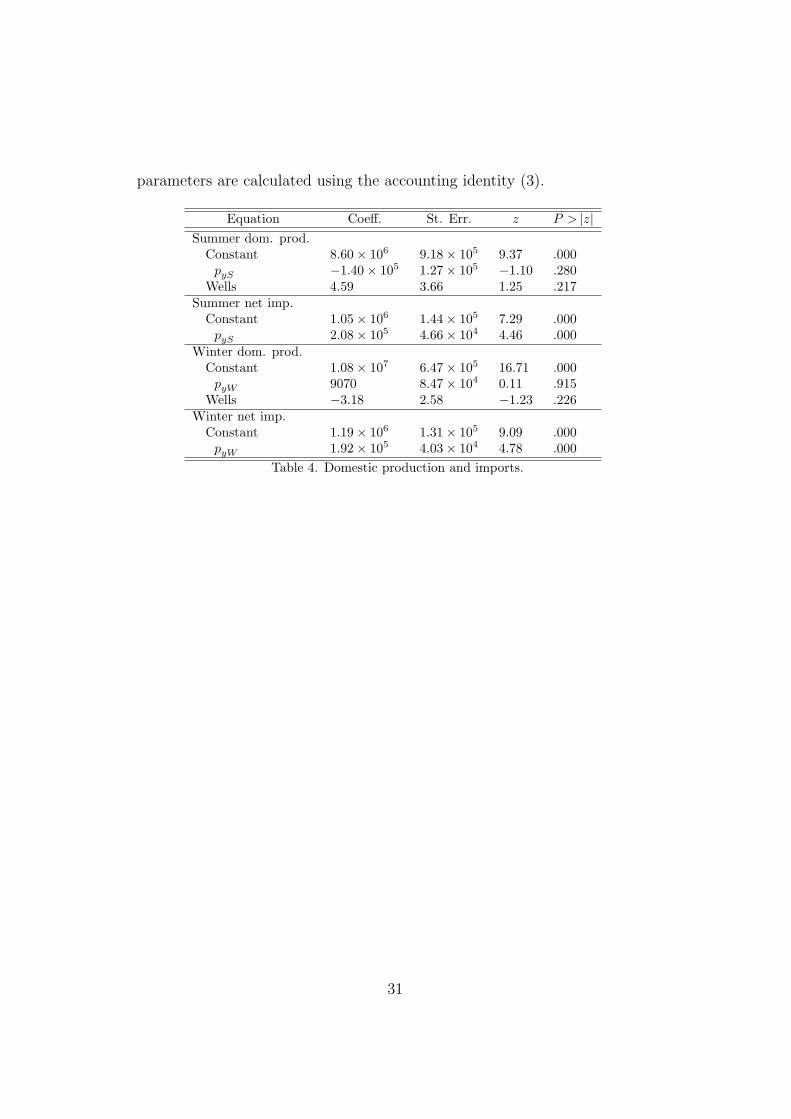
We ran regressions of domestic production and net imports on the currentprice. The results are not stable (exclusion of a particular year or inclusion ofnormally irrelevant explanatory variables have an impact on the estimates)and tend to exhibit excess price elasticity (derived effect of price on demandhas the wrong sign). This happens whether we include the production equa-tions in the previous system (3SLS) or estimate them separately (OLS/2SLS).In contrast, the four core equations (25)-(28) give similar estimates with thethree methods.
One obvious reason for this is that production largely depends on produc-tive capacity, which we thus proxied with the number of active wells givenby the EIA. This indicator does not account for the extreme heterogeneitybetween wells; nevertheless, the predicted price elasticities are now lower,indicating that we are more in line with the short term logic we put forward.Remark that the dynamics of this kind of data is extremely hard to capturein a model.12 We restricted the sample to years 1993 to 2005, the periodbetween 1986 and 1992 having a strong influence on the estimates. See Ta-ble 4 . The small sample cannot warranty precise estimates. In accordancewith economic intuition, the implied price elasticity of demand is now nega-tive; the impact of prices on domestic production is not significant, whereasimports are price-inelastic.
Once domestic production and net import parameters are known, demand
12See the classic Balestra and Nerlove (1966) on the modeling of demand for naturalgas with consideration of the stock of appliances.
30
parameters are calculated using the accounting identity (3).