Source parameter inversion for recent great earthquakes from adecade-long observation of global gravity fields
Shin-Chan Han,1 Riccardo Riva,2 Jeanne Sauber,1 and Emile Okal3
Received 4 September 2012; revised 31 January 2013; accepted 1 February 2013; published 26 March 2013.
[1] We quantify gravity changes after great earthquakes present within the 10 year longtime series of monthly Gravity Recovery and Climate Experiment (GRACE) gravity fields.Using spherical harmonic normal-mode formulation, the respective source parameters ofmoment tensor and double-couple were estimated. For the 2004 Sumatra-Andamanearthquake, the gravity data indicate a composite moment of 1.2� 1023Nm with a dip of10�, in agreement with the estimate obtained at ultralong seismic periods. For the 2010Maule earthquake, the GRACE solutions range from 2.0 to 2.7� 1022Nm for dips of12�–24� and centroid depths within the lower crust. For the 2011 Tohoku-Oki earthquake,the estimated scalar moments range from 4.1 to 6.1� 1022Nm, with dips of 9�–19� andcentroid depths within the lower crust. For the 2012 Indian Ocean strike-slip earthquakes,the gravity data delineate a composite moment of 1.9� 1022Nm regardless of the centroiddepth, comparing favorably with the total moment of the main ruptures and aftershocks.The smallest event we successfully analyzed with GRACE was the 2007 Bengkuluearthquake with M0 ~ 5.0� 1021Nm. We found that the gravity data constrain the focalmechanism with the centroid only within the upper and lower crustal layers for thrustevents. Deeper sources (i.e., in the upper mantle) could not reproduce the gravityobservation as the larger rigidity and bulk modulus at mantle depths inhibit the interiorfrom changing its volume, thus reducing the negative gravity component. Focalmechanisms and seismic moments obtained in this study represent the behavior of thesources on temporal and spatial scales exceeding the seismic and geodetic spectrum.
Citation: Han, S.-C., R. Riva, J. Sauber, and E. Okal (2013), Source parameter inversion for recent great earthquakes froma decade-long observation of global gravity fields, J. Geophys. Res. Solid Earth, 118, 1240–1267, doi:10.1002/jgrb.50116.
1. Introduction
[2] Large-scale processes of geophysical and climate-related mass redistribution cause changes in the gravitationalpotential field. By observing the relative motions of twoidentical satellites (orbiting proof masses), the GravityRecovery and Climate Experiment (GRACE) mission hasbeen mapping the spatial distribution of surface and interiormass flux and transport as well as adjustments in the Earthsystem since its launch in 2002 [Tapley et al., 2005]. Asone of such processes, earthquakes cause variations in thegravitational potential field at a spatial scale up to somethousands of kilometers and at temporal scales of secondsto decades, by radiating seismic energy and deforming thesurface and interior permanently and gradually.
[3] Traditional coseismic and postseismic observationshave measured surface displacements such as ground, sea-floor, and sea-surface motions using a variety of instruments:seismometers, strainmeters, leveling, GPS, InterferometricSynthetic Aperture Radar (InSAR), seafloor transponders,and tsunami gauges. These have been the primary tools usedto understand the rupture dynamics, the spatial extent ofslip, and gradual postseismic changes. However, space-borne gravimetric observations are also sensitive, in partic-ular, to interior deformation in the broader region affectedby the rupture, including the oceanic environment largelyinaccessible by traditional measurements. Specifically, theycould fill in the seldom-observed long wavelength spectrumof earthquake observations as a complement to surfacegeodetic measurements and seismic data. In addition, theyreflect an average deformation over a time window muchlonger than that accessible from seismic data which islimited in principle by the period of the Earth’s gravestmode, 0S2 (3232 s). We examine this new type of earth-quake observations from GRACE gravimetry, which aresensitive to changes in gravitational potential which weexpress in the formalism of the Earth’s normal modes, asan alternative to the study of vertical and horizontaldisplacements, in order to seek additional information onearthquake mechanisms and a new perspective on earth-quake-related processes.
1Planetary Geodynamics Laboratory, NASA Goddard Space FlightCenter, Greenbelt, Maryland, USA.
2Department of Geoscience and Remote Sensing, Delft University ofTechnology, Delft, Netherlands.
3Department of Earth and Planetary Sciences, Northwestern University,Evanston, Illinois, USA.
Corresponding author: S.-C. Han, Planetary Geodynamics Laboratory,NASA Goddard Space Flight Center, Greenbelt, MD, USA ([email protected])
[4] We scrutinize the observations of global gravitationalpotential change after the following recent megathrust earth-quakes: 2004 Sumatra-Andaman (Mw = 9.15 to 9.3), charac-terized by a slip greater than 3m over more than 1200 km offault length [e.g., Tsai et al., 2005; Chlieh et al., 2007]; 2007Bengkulu (Sumatra; Mw = 8.5) [e.g., Borrero et al., 2009];2010 Maule, Chile (Mw = 8.8) with slip greater than 3m over450 km [e.g., Pollitz, et al., 2011]; and 2011 Tohoku-Oki(Mw� 9.0) with slip greater than 5m over 330 km [e.g.,Simons et al., 2011]. In addition to these thrust sources, andfor the first time, we analyze gravitational perturbations dueto the sequence of great strike-slip earthquakes (cumulativeMw� 8.7) which ruptured in 2012 100–200 km southwest ofthe Sumatra subduction zone [e.g., Yue et al., 2012].[5] Such gravity changes are caused dominantly by large-
scale density change in the region surrounding the ruptureand by surface deformation, including interaction with theocean, as suggested by Han et al. [2006] and others there-after. The surface deformation, however, would be expectedto be small in large-scale gravity change for vertical strike-slip earthquakes. Sea level changes due to coseismic gravita-tional potential changes have been addressed more recentlyby de Linage et al. [2009], Broerse et al. [2011], andCambiotti et al. [2011]. While most of these analyses, in-cluding Heki and Matsuo [2010], Matsuo and Heki [2011],and Wang et al. [2012], used the monthly time series ofGRACE gravity maps, Han et al. [2010, 2011] also directlyexploited the fundamental observations of range-rate changeafter earthquakes to optimize spatial and temporal resolu-tion. Han et al. [2011] and Cambiotti et al. [2012] invertedthe GRACE range-rate and monthly gravity data, respec-tively, to quantify the fault parameters of the 2011Tohoku-Oki earthquake. Various numerical modelingapproaches from a half-space [Okubo, 1992] to a layeredspherical Earth model [Pollitz, 1996], considering the oceanlayer and sea level feedback [Broerse et al., 2011; Cambiottiet al., 2011], have been used to compute synthetic gravitychanges. Furthermore, the postseismic gravity change afterthe 2004 Sumatra-Andaman rupture was also identified andsuch observations were interpreted considering the Earth’srheological response to mega-earthquakes [Han et al.,2008; Panet et al., 2010; Hoechner et al., 2011] and thediffusion of water in the mantle [Ogawa and Heki, 2007].[6] In this study, we present a theoretical model of the
coseismic gravitational potential for a spherical Earth on thebasis of gravitational potential normal mode summation, asalso envisaged by Chao and Gross [1987] and de Linageet al. [2009]. We particularly examine the gravitational char-acteristics of normal modes as a function of the Earth’s elasticstructure and the earthquake source depth. We evaluate anddiscuss the effects of surficial layering (including the ocean)and density change on the gravity change. Next, we formulateinverse models to estimate the moment tensor components andsubsequently fault parameters from the GRACE data for eachearthquake. We use the readily available level 2 (L2) dataproducts from the GRACEmission that implies monthly snap-shots of global gravitational potential changes with a spatialresolution of 400–500 km. Finally, we apply this inversionapproach to characterize these earthquakes with (point) cen-troid source representation; discuss the fault solution estimatesof moment, dip, strike, rake and depth, and the trade-offsamong these parameters; and compare these great earthquakes
based on homogeneous data, consistent gravity modeling,and uniform inversion methodology. Although the gradualpostseismic changes after the rupture were also evident inthe data, this study is focused on the coseismic change in thegravitational potential and leaves out the longer-termpostseismic response to a future investigation.
2. Coseismic Gravitational Potential Change Dueto a Double-Couple Source
[7] We derive the expression of coseismic changes ingravitational potential due to a point dislocation on the basisof gravitational potential normal mode summation. Our goalis to obtain the representation in terms of spherical harmoniccoefficients for the coseismic gravitational potential changesas explicit functions of the parameters of a point-sourcedouble-couple (scalar seismic moment M0, dip d, rake l,and strike ff). In the end, we will use these results to analyzeglobal gravity data such as from GRACE to invert earth-quake source processes.[8] The concept that gravity participates in the restoring
force controlling the oscillation of a deformed elastic Earthwas first expressed by Bromwich [1898], following Lamb’s[1882] estimate of its period of free oscillation. Ever sinceLove’s [1911] classical study, which provided the first theo-retical computation of the fundamental mode of a compress-ible, elastic gravitating Earth, all detailed computations ofthe Earth’s normal modes [e.g., Pekeris and Jarosch, 1958;Gilbert and Backus, 1968] have included the relevant varia-tions of its gravitational potential. Because they do not resultin changes in its gravity field, the torsional modes of oscilla-tion of the Earth will be ignored from the rest of this paper.[9] The problem of the excitation of a normal mode by a
seismic source was first described by Alterman et al. [1959]and given a simple and elegant formulation by Gilbert[1970]. This set the stage for the use of normal mode summa-tion to synthesize either seismic waves, which expressthe transient deformation following an earthquake [e.g.,Kanamori and Cipar, 1974] or geodetic displacements, whichexpress permanent coseismic deformation [Pollitz, 1996].Thus, it should be possible to similarly describe any static ortransient changes in the Earth’s gravitational potential on thebasis of a summation of its normal modes. Indeed, this ap-proach goes back to Longman [1962, 1963] in the simpler caseof the loading of the Earth by a point mass.[10] In the notation of Kanamori and Cipar [1974,
Figure 10] and Kanamori and Given [1981, Figure 1], werecall that the radial displacement ur (as would be recordedby a vertical seismometer), excited by a point-source double-couple can be expanded as
ur r; θ;f; tð Þ ¼ M0�Xn;l
y1 rð Þ½�sRK0Pl;0 cos θð Þ þ qRK1Pl;1 cos θð Þ
�pRK2Pl;2 cos θð Þ�� 1� cos nol tð Þ� exp �nol t=2nQlð Þ½ �:
(1)
[11] The definition of the associated Legendre functionsPl,m used here is such that they are normalized to a constantintegral of 4p on the sphere, which relates them to theLegendre functions Pm
l used, for example, by Kanamoriand Cipar [1974] through
HAN ET AL.: EARTHQUAKE SOURCE INVERSION FROM GRACE
1241
Pl;m ¼ffiffiffiffiffiffiffiffiffiffiffiffiffiffiffiffiffiffiffiffiffiffiffiffiffiffiffiffiffiffiffiffiffiffiffik 2l þ 1ð Þ l � mð Þ!
l þ mð Þ!
s�Pm
l ; (2)
where k = 1 is for m = 0 and k = 2 otherwise. The expansionin equation (1) uses a system of spherical harmonics whosepole is chosen at the seismic epicenter, and whose primarymeridian is taken along the dislocation fault strike. Underthis geometry, a point-source double-couple excites onlythe modes of azimuthal orders m = 0, � 1, and � 2, allowingthe expansion (1) to contain only three terms inside the firstbracket; sR, qR, and pR are then trigonometric parametersdepending only on the geometry of the dislocation (dip angled and rake l), and on the longitude f of the receiver, mea-sured from the fault strike [Kanamori and Cipar, 1974,Figure 10]:
sR ¼ sinl sind cosd;qR ¼ sinl cos2d sinfþ cosl cosd cosf;pR ¼ cosl sind sin2f� sinl sind cosd cos2f;f ¼ ff � fr ¼ flon þ ff � p;
(3)
where ff is the azimuth of the fault strike, and fr the azi-muth of the small arc of great circle departing the source tothe receiver, both measured clockwise from local north atthe epicenter (alternatively, fr =p�flon, where flon wouldbe the longitude of the receiver in a frame where the pole isat the epicenter, measured counterclockwise from the direc-tion of local south at the source). y1 is the vertical displace-ment component of the eigenfunction (dependent on degree land overtone number n) [Alterman et al., 1959; Saito, 1967].The functions K0, K1, and K2, of which explicit forms aregiven in Kanamori and Cipar [1974], describe the excitationof a full Earth oscillation by a seismic source, as such de-pends only on l and n as well as on the specific Earth modelused, and of course on the depth ds of the source, but nolonger on the particular orientation of either the source orthe receiver. The temporal part expressed as the secondbracket of equation (1) consists of a static term describingthe permanent deformation of the Earth (expressed as the“1” in the bracket) and of a transient oscillatory term “seismicwaves” corresponding to the attenuated sinusoid. An equiva-lent expression using moment tensor components can befound in Kanamori and Given [1981] and Pollitz [1996].
[12] This formalism can be extended immediately to thecase of the variations in gravitational potential c(r,θ,flon)by replacing the first component y1 of the eigenfunction bythe fifth one, y5, as introduced by Alterman et al. [1959].In the particular case of the permanent “static” variation ofthe potential at the Earth’s surface (r= a), one simply obtains
c θ;flonð Þ ¼ M0�Xn;l
y5 að Þ�½�sRK0Pl;0 cos θð Þ
þqRK1Pl;1 cos θð Þ � pRK2Pl;2 cosθð Þ�:
(4)
[13] Note that y5 is computed routinely as part of the solu-tion of the full elastogravitational eigenproblem of the freeoscillation and that its inclusion is particularly critical to theaccurate determination of the period of the gravest modes, inparticular, the radial ones (l=0). However, the informationcontained in y5 has rarely been used, since most applicationsof normal mode theory have been limited to seismology,before the advent of detailed large-scale gravity observations,notably with programs such as GRACE [Tapley et al., 2005].[14] By substituting equation (3), equation (4) can be re-
written as follows:
c θ;flonð Þ ¼ GM
a
Xl
X2m¼0
Pl;m cosθð Þ Cl;m cosmflon þ Sl;m sinmflon
� �;
(5)
where G is the universal gravitational constant, M the massof the Earth, and a its radius. The five non-trivial dimension-less coefficients are defined, with the moment tensor compo-nents following the convention by Aki and Richards [1980]as follows:
Cl;0 ¼ a
GM
Xn
K0 dsð Þy5 að Þ" #
� �Mrr
2
� �; (6a)
Cl;1 ¼ a
GM
Xn
K1 dsð Þy5 að Þ" #
� Mrθð Þ; (6b)
Sl;1 ¼ a
GM
Xn
K1 dsð Þy5 að Þ" #
� Mrf� �
; (6c)
Cl;2 ¼ a
GM
Xn
K2 dsð Þy5 að Þ" #
� Mθθ �Mff
2
� �; (6d)
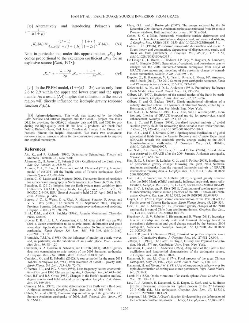
(a) (b) (c)
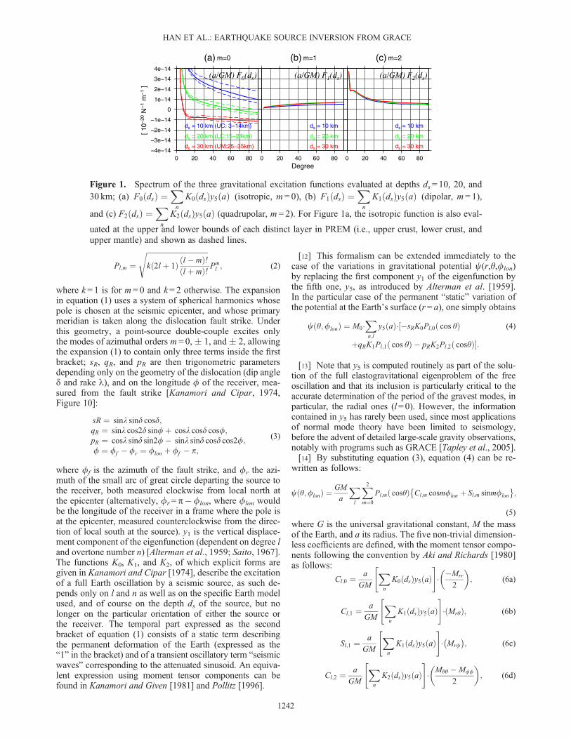
Figure 1. Spectrum of the three gravitational excitation functions evaluated at depths ds= 10, 20, and30 km; (a) F0 dsð Þ ¼
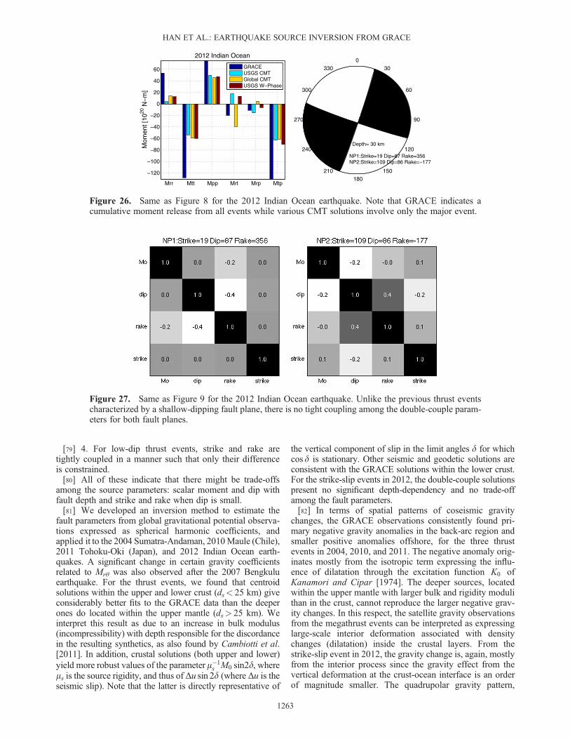
Xn
K0 dsð Þy5 að Þ (isotropic, m = 0), (b) F1 dsð Þ ¼Xn
K1 dsð Þy5 að Þ (dipolar, m= 1),
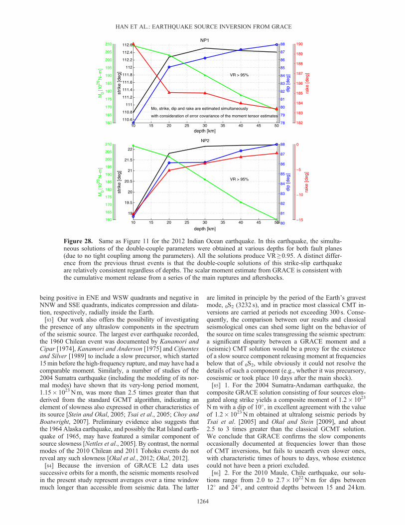
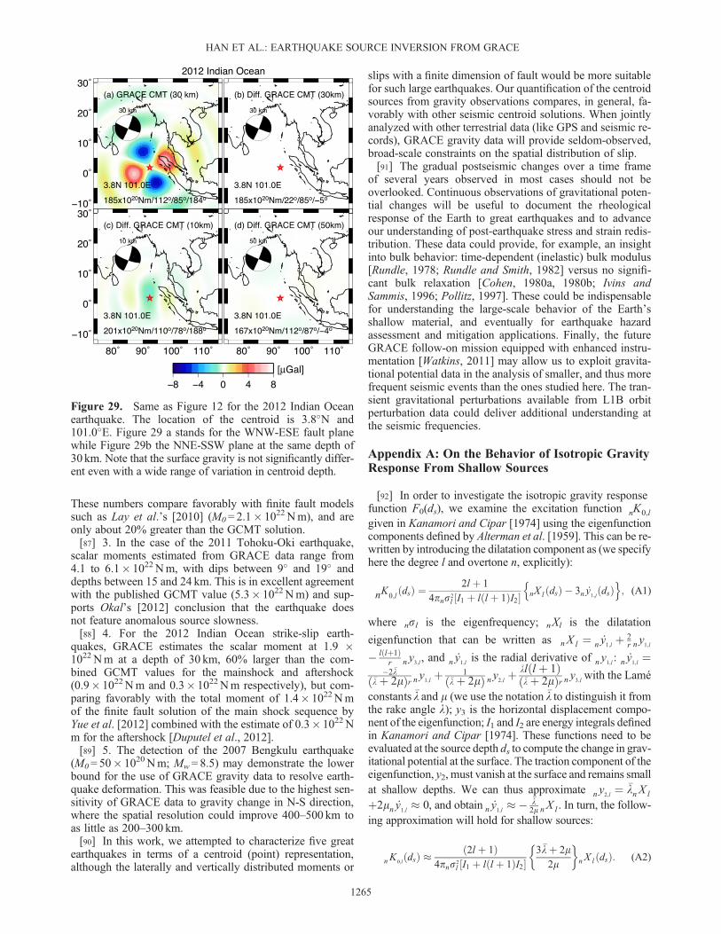
and (c) F2 dsð Þ ¼Xn
K2 dsð Þy5 að Þ (quadrupolar, m = 2). For Figure 1a, the isotropic function is also eval-
uated at the upper and lower bounds of each distinct layer in PREM (i.e., upper crust, lower crust, andupper mantle) and shown as dashed lines.
HAN ET AL.: EARTHQUAKE SOURCE INVERSION FROM GRACE
[15] In equation (6) and for each value of degree l, the sum-mations in the functions Fm ¼
Xn
Km dsð Þy5 að Þ, (m=0, 1, 2)
are performed over the overtone number n on which the indi-vidual values of y5(a) and the Km(ds) will of course depend. Inparticular, these functions of l are now characteristic of the(laterally homogeneous) Earth model, but no longer dependon any property of the seismic source (excluding depththrough the Km(ds)), and as such, they can be precomputedfor any combination of l and ds.[16] These functions are closely related to the coefficients
ylm Sð Þ1 used to expand radial deformation by Pollitz [1996,equation (3a)], except that we express them with sines andcosines as opposed to imaginary exponentials and thatPollitz [1996] considered only elastic (and not gravitational)restoring forces. Pollitz [1992] showed in considerable detail(including the effect of gravity) that it is possible to computedirectly the functions Fm from the equations of equilibriumof the deformed Earth, rather than explicitly summing overan a priori infinite number of overtones n, as in equation(6). We follow here an approach similar to Piersantiet al.’s [1995] and Pollitz et al.’s [2006] studies, which con-sists of casting the static problem of the equilibrium of a lay-ered gravitating elastic Earth in the same formalism as thedynamic one for a free oscillation, but of course in the ab-sence of any time-dependent terms, following in the foot-steps of Longman [1963] and Smylie and Mansinha [1971].[17] In this framework and given a point-source double-
couple of prescribed geometry and amplitude (M0), imbeddedat the depth ds in an elastic Earth, Pollitz’ [1996] formal-ism consists of expanding its field of discontinuities(obtained under a representation theorem) onto sphericalharmonics, and of defining, for each degree l and ordersm=0, 1, and 2, an equivalent discontinuity at the depth ds inthe four components of the eigenvector y of the static problem(which remains independent of m). In the presence of gravity,we generalize it by imposing the continuity of the additionalcomponents, y5 and y6, for r= rs (rs= a� ds), thus imposingsix boundary conditions on the full six-dimensionalelastogravitational eigenvector y. Following Pollitz et al.[2006] and because y is continuous at all depths d 6¼ ds, exceptat the core-mantle boundary as discussed for example bySmylie and Mansinha [1971], it can be integrated continu-ously upwards to r ¼ r�s from the core-mantle boundary,where initial conditions feature three degrees of freedom,detailed for example by Vermeersen et al. [1996], in theframework of Chinnery’s [1975] explanation of the so-calledLongman’s paradox. Similarly, it can be integrated from thesurface of the Earth (where there are again three degrees offreedom) downwards to rþs . For each m=0, 1, and 2, the six
boundary conditions at r= rs define the proper combinationof initial conditions from which the value of y5(a) can be com-puted and equated to Fm.[18] As mentioned above, equations in (6) are relatively
simple because they are written in a particular system ofspherical harmonics, where the pole is at the seismic epicen-ter and the prime meridian oriented along the local south,since under this geometry, a point-source double-couple ex-cites only azimuthal orders m = 0, � 1, and � 2. That framewill hereafter be identified with a superscript s. However,when studying the gravity field of the Earth, the conventionis to use the geographic spherical harmonics, defined aboutits axis of rotation (the North Pole) and the prime Greenwichmeridian, hereafter be identified with a superscript g. There-fore, one has to project one system of spherical harmonicsonto the other, in order to express equation (6) in the geo-graphic harmonics; this relatively classical problem [e.g.,Sato, 1950; Brink and Satchler, 1968; Stein and Geller,1977] is carried out as a succession of two solid rotations:The first one (of amplitude θs, the colatitude of the epicenter)is taken about the pole of the geographic meridian goingthrough the epicenter and brings back the pole of the spher-ical harmonics to the geographic North Pole, and the secondone (of amplitude�fs, the opposite of the longitude of theepicenter) is taken about the axis of rotation of the Earthand restores the Greenwich meridian as the primary one.[19] Regrouping the coefficientsCl,i and Sl,i in equation (6) in
the form of a vectorXsl (X
sl;�2 ¼ Sl;2, X s
l;�1 ¼ Sl;1, X sl;0 ¼ Cl;0,
X sl;1 ¼ Cl;1, andX s
l;2 ¼ Cl;2), the projection onto the geographicharmonics is expressed as a new vector Xg
l :
X gl;m M0;ff d; l; ds; θs;fs
¼
X2i¼�2
Elm;i θs;fsð ÞX s
l;i M0;ff d; l; ds
�l≤m≤l; (7)
where the factor E expresses the combination of two rotations.Note that despite its apparent complexity, equation (7) remainsa completely linear operation on the various components ofthe vector Xs
l .[20] A fundamental aspect of equation (7) is that while the
potential field resulting from a dislocation expressed as apoint-source double-couple could be expanded on harmonicsof orders m= 0, � 1, and � 2 in the source-based system(Xs
l being five-dimensional), it will project on all orders(�l ≤m ≤ l) in the geographic system centered at the NorthPole (Xg
l being (2 l + 1)-dimensional). Note that a similar ap-proach is used when studying the splitting of the free oscil-lations of the Earth due to rotation and ellipticity, with theidentical result that normal modes excited by an earthquakeare split into all of their (2 l + 1) singlets (�l ≤m ≤ l ) [Steinand Geller, 1977].
3. Coseismic Gravitational Response Functions
[21] We characterize the coseismic changes in gravita-tional potential c through the functions
Fm dsð Þ ¼Xn
Km dsð Þy5 að Þ; (8)
with orders m= 0, 1, 2 for isotropic, dipolar, and quadrupolarexcitations, respectively. They represent the Earth’s gravi-metric response to faulting by a double-couple and depend
HAN ET AL.: EARTHQUAKE SOURCE INVERSION FROM GRACE
1243
only on Earth structure, degree l, and source depth ds. Figure 1presents examples of these functions, computed for the Pre-liminary Reference Earth Model (PREM) model [Dziewonskiand Anderson, 1981] at three representative depths (10, 20,and 30 km), sampling the upper crustal (3–15 km), lowercrustal (15–24 km), and upper mantle (24–80 km) layers ofthe model.[22] As shown in Figure 1, the behavior with l of the three
functions is significantly different. Both F1 and F2 areweakly dependent on depth and monotonic (respectively, in-creasing and decreasing functions of l) functions, while F0
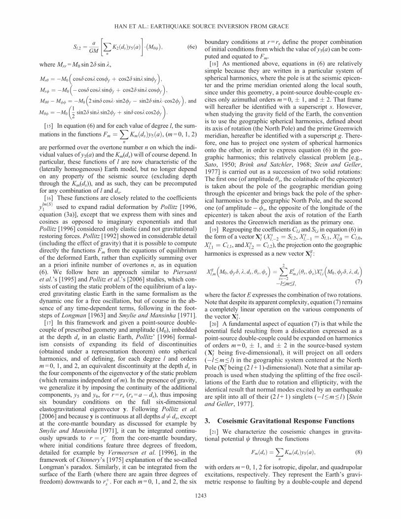
strongly depends on depth, to the extent that it even reversessign, with the nodal degree decreasing with increasingdepth. This strong dependence of F0 on depth is further in-vestigated by computing its values at the upper and lowerbounds of each source layer, shown as dashed lines onFigure 1a; they suggest a moderate dependence of F0 withdepth within a layer, but a significant one between layers,which illustrates the critical dependence of the coefficientsK0 on the elastic moduli at the source. The spatial patternof Fm at different depths is shown in Figure 2, truncated atdegree 50 (i.e., spatial resolution of 400 km). The isotropicterm, F0, is dominant when the source is at the lower depth,while the non-isotropics, F1 and F2, become more pro-nounced as the source depth increases.[23] Several features of Figures 1 and 2 are straightfor-
ward to interpret in the context of classical results of normalmode seismology. In particular, we recall that the strike-slipcoefficient K2 is proportional to y3/rs. In the vicinity of theEarth’s surface, where the shear stress y4 vanishes, the
logarithmic derivative of this quantity takes the valuery3� ddr y3
r
� � ¼ � 1ry1y3� � l
auzux, on the order of � l/a for l> 1,
and for branches of modes featuring a reasonably circularground motion at the surface (e.g., fundamental Rayleighwaves for which this ratio approaches 1.5). Thus, the charac-teristic depth for the decay of K2 near the surface is on theorder of a/l, which means that K2 is essentially independentof depth for shallow earthquakes, a well-known property ofmantle Rayleigh waves. This explains the lack of depen-dence of F2 on depth, as exhibited in Figure 1c. By contrast,the coefficient K1, proportional to y4/m, vanishes at the sur-face, leading to the classical singularity in excitation bydip-slip components at shallow depths [e.g., Kanamori andGiven, 1981]. For shallow sources (ds much less than onewavelength), y4 is expected to be continuous and grow line-arly with depth; however, m will suffer discontinuities in thevarious layers of the Earth, leading to a much slower growth(or even an irregular behavior) of K1 with depth. As for theisotropic coefficient K0, involved (together with K2) in thecase of a dipping (e.g., thrust) fault, its more complex ex-pression as a function of the eigenvector y precludes anysimple interpretation of its variation with depth.[24] The physical origin of the change in gravitational po-
tential at the surface, y5(a), can be separated into two contri-butions, namely (i) a displacement of the free boundary ofthe Earth, resulting in the filling of an initially void volumeby material of finite density and (ii) the effect on c at the sur-face of changes in density within the interior of the planet,resulting from its deformation, including that of surfaces of
Figure 2. Spatial patterns of the functions Fm(ds) in the vicinity of the source, evaluated at depths of 10,20, and 30 km.
HAN ET AL.: EARTHQUAKE SOURCE INVERSION FROM GRACE
1244
discontinuity, such as the crust-mantle interface. For (ii), thegravitational effect of the (coseismic) change of discontinu-ity in interior density stratification is considerably smallerthan the interior density change by compression and/or dila-tation [Pollitz, 1997; Han et al., 2006]. In the limit of large-scale gravity changes (a few 100 km), the effect from (ii) isas large as (i), while (i) overwhelms (ii) at much smallerscales, as shown in Han et al. [2006].[25] The change in gravitational potential due to the defor-
mation of the surface, F Bð Þm , is in the nature of a Bouguer
effect, and can be easily computed from the radial dis-placement component of the eigenvector, y1(a). In the limity1< a/l (i.e., the vertical deformation being smaller than itslateral dimension), the contributing material can be modeledas a thin layer of thickness y1 and density Δr (crustal densityfor inland earthquakes, reduced by seawater density forundersea ones), leading the classical result [Jeffreys, 1976;Turcotte et al., 1981]:
F Bð Þm ¼
Xn
Km dsð Þ 4pGaΔr2l þ 1ð Þ y1 að Þ; m ¼ 0; 1; 2: (9)
[26] The degree-dependent scale factor multiplying the y1eigenfunction is needed to convert the thin layer mass anom-aly Δry1(a) into the gravitational potential anomaly at thesurface. The contribution from the interior deformation(mostly due to coseismic dilatation or compression of thematerial surrounding the source) is computed by removingthis superficial (or Bouguer) contribution from the full vari-ation Fm as
F Ið Þm ¼ Fm � F Bð Þ
m
¼Xn
Km dsð Þ y5 að Þ � 4pGaΔr2l þ 1ð Þ y1 að Þ
� �; m ¼ 0; 1; 2: (10)
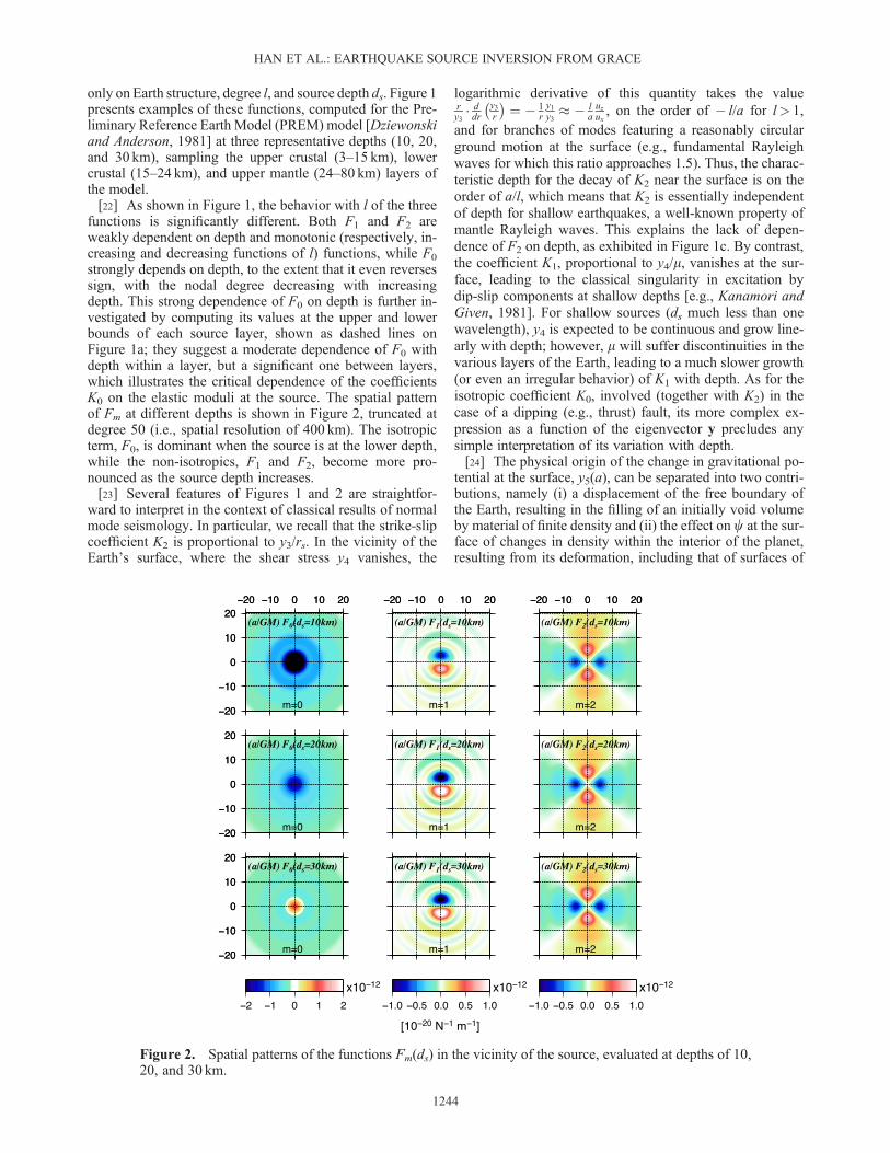
[27] Although we did include self-gravitation and loadingwhen computing the functions Fm and for the sake of simplic-ity, they are not discussed here, as their contributions are con-siderably smaller than the simple Bouguer effect expressed byequation (10); see de Linage et al. [2009] and Cambiotti et al.[2011] for details. The degree-dependent behaviors ofequations (9) and (10) at three different depths are shown inFigure 3, where the sign for the surface deformation functionform=0 was reversed in the plot. As for the case of total grav-ity change in Figure 1, the depth-dependence is found to be
significant in the isotropic case, where the interior deformationshows even greater depth-dependence. For the isotropic com-ponent, which is directly related to dilatation at the source (see
Appendix A), the interior deformation F Ið Þ0 ; m ¼ 0ð Þ contrib-
utes more signal than the Bouguer term F Bð Þ0 when the source
locates at shallower depth (10 km, within the upper crust)
where the material is more compressible. In contrast, F Bð Þ0 be-
comes prominent when the source is deeper (i.e., 30 km,within the upper mantle) where the material is less compress-ible. In the dipolar case (m=1), the change in potential is
largely due to the Bouguer term F Bð Þ1 at all depths, while in
the quadrupolar case (m=2), F Ið Þ2 remains prominent at all
depths.[28] We computed the coseismic potential change from a
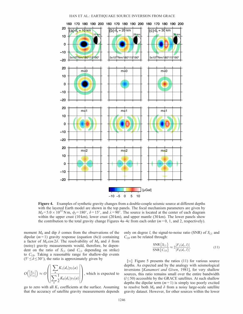
synthetic double-couple at different depths (using a com-pressible Earth model with an ocean layer). A centroid witha scalar moment M0= 5.0� 1022Nm (Mw= 9.0) and strikeff= 180�, dip d = 15�, and rake l= 90� was used. Thegravity changes (up to degree and order 40, or equivalentlya spatial resolution of 500 km) from the same seismic sourcebut at different depths are compared in Figure 4. The effectof the isotropic term (m = 0), mostly responsible for a largecentral negative anomaly, decreases with increasing depthsand, as a result, the other terms (m = 1, 2) that are relativelyconstant with depth become more prominent in the totalcoseismic gravity change.
3.1. Moment Dip Trade-off
[29] It has been long known in the seismological commu-nity that the inversion of seismic moment tensors suffers asingularity for shallow sources [e.g., Kanamori and Given,1981]. This is due to the fact that the dipolar coefficientK1, proportional to the shear stress y4, vanishes at the surfacewith the result that the two components Mr’ and Mrθ do notexcite seismic modes at or near the surface. Conversely, theycannot be resolved for a surficial source (or are poorly re-solved for a shallow source) from seismograms. This classi-cal singularity results in a trade-off between scalar momentM0 and dip angle d.[30] For thrust earthquakes (l� 90�), the observations of
isotropic (m = 0) and quadrupolar (m= 2) gravity response(equations (6a) and (6d)) constrain only M0 sin 2d. Thecomplementary information required to separate the scalar
(a) (c)(b)
Figure 3. Same as Figure 1, with function Fm(ds) separated into their surface (F Bð Þm ) and interior (F Ið Þ
m )contributions to the total gravitational potential. Note that the sign of F Bð Þ
0 (shown as solid line) has beenreversed in Figure 3a for plotting clarity.
HAN ET AL.: EARTHQUAKE SOURCE INVERSION FROM GRACE
1245
moment M0 and dip d comes from the observations of thedipolar (m= 1) gravity response (equation (6c)) containinga factor of M0 cos 2d. The resolvability of M0 and d from(noisy) gravity measurements would, therefore, be depen-dent on the ratio of Sl,1 (and Cl,1 depending on strike)to Cl,0. Taking a reasonable range for shallow-dip events(5� ≤ d ≤ 30�), the ratio is approximately given by
O Sl;1Cl;0
��� ��� � O
Xn
K1 dsð Þy5 að ÞXn
1
2K0 dsð Þy5 að Þ
����������������
0BB@1CCA, which is expected to
go to zero with all K1 coefficients at the surface. Assumingthat the accuracy of satellite gravity measurements depends
only on degree l, the signal-to-noise ratio (SNR) of Sl,1 andCl,0 can be related through:
SNR Sl;1� �
SNR Cl;0
� � � 2F1 ds; lð ÞF0 ds; lð Þ���� ����: (11)
[31] Figure 5 presents the ratios (11) for various sourcedepths. As expected and by the analogy with seismologicalinversions [Kanamori and Given, 1981], for very shallowsources, this ratio remains small over the entire bandwidth(l ≤ 50) accessible by the GRACE satellites. At such shallowdepths the dipolar term (m = 1) is simply too poorly excitedto resolve both M0 and d from a noisy large-scale satellitegravity dataset. However, for other sources within the lower
(a) (c)(b)
Figure 4. Examples of synthetic gravity changes from a double-couple seismic source at different depthswith the layered Earth model are shown in the top panels. The focal mechanism parameters are given byM0= 5.0� 1022Nm, ff= 180�, d = 15�, and l = 90�. The source is located at the center of each diagramwithin the upper crust (10 km), lower crust (20 km), and upper mantle (30 km). The lower panels showthe contribution to the total gravity change Figures 4a–4c from each order (m= 0, 1, and 2, respectively).
HAN ET AL.: EARTHQUAKE SOURCE INVERSION FROM GRACE
1246
crust and the upper mantle, SNR{Sl,1} becomes comparableto SNR{Cl,0}, likely allowing the resolution of M0 and dfrom the GRACE gravity observations.
4. Observations of Global Gravity Field andSpatial Localization
[32] As part of the GRACE project, one month’s worth oforbital tracking data of the GRACE satellites have been rou-tinely analyzed to obtain an “average” snapshot of the globalgravity field at each month since April 2002. Such a snapshotis represented by and provided as a set of spherical harmoniccoefficients, known as L2 product. In this study, wewill exam-ine those L2 spherical harmonic coefficient data from April2002 to September 2012. The L2 data have been continuouslyupdated with the improved processing strategy and back-ground models including atmosphere and ocean variability.We used the most recent Release-5 (RL5) L2 data productexcept for 2002, for which the Release-4 (RL4) product wasused, since the RL5 product has, at present, not yet beenprocessed for these years [Bettadpur et al., 2012].[33] The coseismic gravitational perturbation tends to be
spatially localized around the epicenter, and thus, its energyis smeared out among all spherical harmonic coefficients.Due to other gravitational variations from continental-scalemass variations (mainly in association with seasonal climatechanges), the earthquake signal may not be apparent directlyfrom the L2 data. Such “local” signal can be better delin-eated from the “global” spherical harmonic coefficients byapplying a spatial window around the region of interest.Simons et al. [1997] and Wieczorek and Simons [2005]developed an optimal windowing function to extract the spa-tially confined signal by minimizing the spatial truncation(leakage) effect. Han and Simons [2008] applied this tech-nique successfully to identify the 2004 Sumatra-Andamanearthquake signal out of the spherical harmonic coefficientsfrom GRACE. Han and Ditmar [2008] discussed howthe SNR of non-stationary signals may be substantiallyunderestimated, if not localized, and suggested a better
way to quantify the SNR of the local signal from the spher-ical harmonic coefficient data under stationary noise.[34] The optimal spatial windowing function h(θ), often iso-
tropic and band-limited, is found by maximizing its energywithin a confined region of interest [Wieczorek and Simons,2005]. Once the windowing function is determined, one canobtain spherical harmonic coefficients of the spatially local-ized signals using a “convolution-like” formula provided inequation (10) of Wieczorek and Simons [2005] and given as:
where Lh is the maximum expansion degree of thewindowing function and hj is the expansion coefficients ofthe zonal (isotropic) window h(θ). The last two parenthesesare Wigner-3j functions. Cim is the (original) sphericalharmonic coefficient and Ch
lm is the localized coefficienthighlighting the signals over the region.[35] As implied by equation (12), the coefficient of the
localized (or windowed) signal is nothing but a linear combi-nation of the original coefficients with the weights definedby the choice of the windowing function. The localized coef-ficient of degree l is computed with the original coefficientswithin the bandwidth [max(0, l� Lh), (l+Lh)]. If the originalsignal is known only to a certain degree such as Ls, it can bereadily seen from the upper bound of the summation inequation (12) that the permissible range of the localized coef-ficients is limited to Ls�Lh. Also the windowed spectra of thelow degrees (l< Lh) can be biased as noted in Section 5.1 ofWieczorek and Simons [2005]. Therefore, we use the localizedspherical harmonic coefficients within the bandwidth, Lh+1to Ls�Lh, from monthly GRACE L2 data.[36] Figure 6 shows signals for recent great earthquakes
(the 2004 Sumatra-Andaman, 2007 Bengkulu, 2010 Maule(Chile), 2011 Tohoku-Oki, and 2012 Indian Ocean events)that are in a detectable range with GRACE gravity data.The spatial maps of coseismic gravity change computedfrom Global Centroid Moment Tensor (GCMT) solutionsof each respective event are shown in Figures 6a-6e, withthe spherical circle that delineates the area of localizationwith the spherical cap of radius θh. The cross section of eachspatial windowing function is shown in Figures 6f–6j,respectively. The relative amplitude is presented over thespherical angular distance θ from the center of the cap.The expansion degree Lh is fixed at 20 and the cap radiusθh is chosen to capture most of the (expected) coseismicgravity signal, mainly depending on the size of the earthquake.This provides the only optimally localized windowing func-tion for each earthquake (that is, the Shannon number is equalto 2 as in Wieczorek and Simons [2005]). The amplitude ofeach windowing function becomes approximately 1% of themaximum amplitude beyond the spherical cap of radius θh,indicating that h(θ) is nearly perfectly concentrated withinthe spherical cap. The concentration ratio g, showing howmuch power of the window function is concentrated withinthe spherical cap, approaches 99% for all cases.[37] The temporal variability (in terms of root-mean-square,
RMS) of the monthly GRACE L2 data, after localization isapplied in the respective areas, is shown in Figures 6k–6o,
0
1
2
3
0 20 40 60 80
ds = 5 km
ds = 10 km
ds = 20 km
ds = 30 km
Degree
Figure 5. Ratio of the dipolar gravity response F1(ds) tothe isotropic response F0(ds) as function of degree l. This ra-tio characterizes the resolvability of moment from dip anglewhen inverting gravity observations, as a function of degreel for various source depths.
HAN ET AL.: EARTHQUAKE SOURCE INVERSION FROM GRACE
1247
for each earthquake, within the bandwidth, Lh + 1 to Ls�Lh(i.e., from 21 to 40 in our case since Ls = 60 and Lh = 20).This is suggestive of inherent temporal variability of thegravity field (mass redistribution) in each region and of theobservational noise. The gravity signal strength predictedfrom GCMT solution of each event is also depicted afterthe same localization is applied. The ratio of the (predicted)coseismic gravitational perturbation to the GRACE datavariability approaches 6, 0.5, 1, 3, and 1.5, respectivelyfor each event, within most of the bandwidth from degrees21 to 40. In Section 6, we will examine the time series ofthese localized L2 coefficient observations and invert themto determine the fault parameters of each earthquake.
5. Linear and Nonlinear Inversion
[38] So far, we examined the forward model of the gravi-tational potential change in response to a point-source
double-couple, expressed in terms of the moment tensor asin equation (6) and in particular, its dependence on depth.The spatial localization of global GRACE gravitationalpotential data was introduced for identifying and analyzingcoseismic gravity changes around various earthquakeregions. In this section, we discuss how we determine themoment tensor from the “localized” GRACE data and, sub-sequently, invert the double-couple source parameters fromthe moment tensor solutions.
5.1. Linear Estimation of Moment Tensor from GravityData
[39] The estimation of the moment tensor componentsfrom a series of geopotential observations is straightforwarddue to its linearity, when the data are expressed in terms of aseries of spherical harmonic coefficients, as discussed inSection 2. In order to invert the dataset of localized GRACEgravitational potential coefficients into the moment tensor m,
(a)
(f) (g) (h) (i) (j)
(k) (l) (m) (n) (o)
(b) (d)(c) (e)
Figure 6. (a–e) Synthetic gravity changes computed from centroid moment tensor (CMT) solutions for the2004 Sumatra-Andaman, 2007 Bengkulu, 2010 Maule, 2011 Tohoku-Oki, and 2012 Indian Ocean earth-quakes, respectively. The black circle delineates the spherical cap of radius θh as the region of localizationwhere the spatial windowing function h(θ) is concentrated; (f–j) cross sections showing the relative amplitudeof h(θ), expanded to degree 20 (Lh= 20), but with a different cap radius (θh) for each event; (k–o) degree RMSspectrum (square root of power spectrum in mGal) of synthetic coseismic gravitational potential (blue line)and of average variability of monthly GRACEL2 data (red line) after applying an identical spatial windowingfunction in each region. The data variability (red line) includes the gravity signal variability (e.g., seasonalchange) as well as the GRACE instrument noise. The ratio of the (predicted) coseismic gravitational pertur-bation to the GRACE data variability approaches 6, 0.5, 1, 3, and 1.5, respectively for each event.
HAN ET AL.: EARTHQUAKE SOURCE INVERSION FROM GRACE
1248
we express the forward problem as a succession of threeoperations.[40] First, as expressed in equation (6), we multiply the
tensor of Green’s functions evaluated at the seismic sourcedepth ds by the moment tensor:
Xs ¼ F dsð Þm; (13)
where F(ds) regroups, for all used values of l, the fivefunctions Fm discussed in Section 3;m = (Mrr,Mrθ,Mrf,MθθMff�Mθf) represents the five independent unknown mo-ment tensor components; the resulting vector Xs regroups,for all values of l, the spherical harmonic coefficients inequation (6). Second, we apply the rotations expressing thechange of frames, and obtain
Xg ¼ R θs;fsð ÞXs; (14)
where the dimension of the vector Xg is the sum of (2l + 1)over the range [lmin, lmax] used in the inversion, and R(θs,fs) is a rotation matrix consisting of all the elementsElm;i of equation (7). Third, the spatial localization discussed
in Section 4 is applied, leading to
XL ¼ L θs;fsð ÞXg; (15)
where L(θs,fs) is a matrix expressing the operation inequation (12).[41] At this point, XL regroups the gravitational potential
coefficients expressed in the geographic frame, and localizedaround the epicenter (θs,fs), as excited by the double-couplesource described by m. The inversion then consists of usingthe GRACE dataset of observed coseismic change in gravi-tational potential x (itself expended onto spherical har-monics) to solve for m through
L θs;fsð Þx ¼ L θs;fsð ÞR θs; ;fsð ÞF dsð Þmþ e; (16)
where e is the noise in the GRACE dataset. Note that L ap-pears on both sides of (16) because e is determined onlywhen the localized data Lx is sought from noisy time seriesof GRACE data. Finally, simple least squares is used to de-termine the estimate of the moment tensor components, m̂,and its covariance matrix, Cfm̂g.
5.2. Nonlinear Estimation of Double-Couple FromMoment Tensor
[42] The determination of double-couple source parameters(i.e., M0, ff, d, and l) from moment tensor components con-sists of solving backwards the equations in (6). While point-source double-couples are characterized by four parameters,they do not constitute a four-dimensional vector space, andmoment tensor inversions have to be carried out in a five-dimensional vector space, fostering both nonlinearity andnon-uniqueness. We use a standard approach in seismologyto derive two nodal plane solutions of strike, dip, and rakeby using a computer code (bb.m, a Matlab code written byOliver Boyd, based on mij2d.f, a FORTRAN code by Chen Ji)available from the website [www.ceri.memphis.edu/people/oldboyd/Software/Software.html]. They are used as initial so-lutions for our refined inversion considering variable uncer-tainties in moment tensor components as described below.[43] First of all, we examine correlation among the fault
parameters. For low-dip (d� 0) earthquakes as in most
of cases in this study, the moment tensor components areapproximated (to the first order) to Mrr�M02d sin l,Mrθ��M0 cos(ff� l), Mrf�M0 sin(ff� l), Mθθ�Mff ��M02d sin(2ff� l), and Mθf��M0d cos(2ff� l). It indi-catesMrθ andMrfwould be dominant andff� l (not individ-ually) would be better-constrained from the moment tensor.The parameters such as ff and l would be tightly coupled ina manner that ff� l is constant. Han et al. [2011] discussedthis trade-off between strike and rake found from variousseismic solutions and GRACE data inversion for the 2011Tohoku-Oki earthquake.[44] The correlation among double-couple parameters can
be quantified by examining a covariance matrix of thedouble-couple solution. We derive it by introducing a smallperturbation in the double-couple parameters as follows:
M0 ¼ eM0 1þ d�ð Þ; (17a)
ff ¼ eff þ dff ; (17b)
d ¼ edþ dd; (17c)
l ¼ elþ dl: (17d)
[45] The perturbation in the vector of moment tensor com-ponents Δm due to perturbation in double-couple parametersd is simply written as Δm�Bd, where B is a matrix
consisting of partial derivatives, e.g., dMrrd� ,
d Mθθ�Mffð Þdd , evalu-
ated for nominal values of eM0,ed,el, and eff . The Δm includes,e.g., ΔMrr, andΔ(Mθθ�Mff), and finally d consists of d�,dd, dl, and dff. Therefore, the covariance matrix of the
double-couple parameters, Cfd̂g, is computed from the co-variance matrix of the moment tensor solution, C m̂
� �, by
error propagation:
C d̂n o
¼ BT C m̂n oh i�1
B
� �1
: (18)
[46] The correlation matrix is simply computed by re-
scaling all elements of Cfd̂g by ri;j ¼ ci;j=ffiffiffiffiffiffiffiffiffiffiffici;icj;j
p, where
ci,j is a component of the i-th row and j-th column of thematrix. This is a metric we examine using the initial faultplane solutions from moment tensor estimates for all earth-quakes in this study.[47] The (iterative) least square refinement to the initial
solution of eM 0, ed, el, and eff , (available from the eigenvalueand eigenvector decomposition of the moment tensor matrix,
i.e., from the code bb.m), is found by d̂ ¼ Cfd̂gBT
Cfm̂gh i�1
m̂ � emð Þwhere em is a moment tensor component
vector computed with the initial double-couple parameters.This solution takes care of the variable uncertainties andcorrelation in the moment tensor estimates from GRACE.Depending on the correlation structure among four param-eters computed with equation (18), this solution may needto be constrained. We will elaborate on this procedure foreach of the earthquakes in Section 6.[48] We do not attempt to solve for the centroid location
(θs,fs) and depth ds because their dependence on gravity
HAN ET AL.: EARTHQUAKE SOURCE INVERSION FROM GRACE
data, as expressed in equation (16), is algebraically complex.However, we test various depths ds, and at each depth, wesolve for the corresponding moment tensor and the bestdouble couple. We adopt the centroid location (θs,fs) deter-mined from other seismic CMT or finite fault solutions.
6. Inversion for Moment Tensor and FaultParameters
6.1. 2004 Sumatra-Andaman Earthquake
[49] We analyzed the entire time series of monthly globalgravity fields from April 2002 to September 2012 (in termsof spherical harmonic coefficients) in order to separate, inthe data obtained after the rupture, the gravity signal dueto the earthquake from the background temporal variation inthe gravity potential. We fit the time series using the mean,annual and semiannual sinusoids, and a Heaviside step(for coseismic) and a logarithmic function (for postseismic)
simultaneously. The logarithmic term, log 1þ t150 days
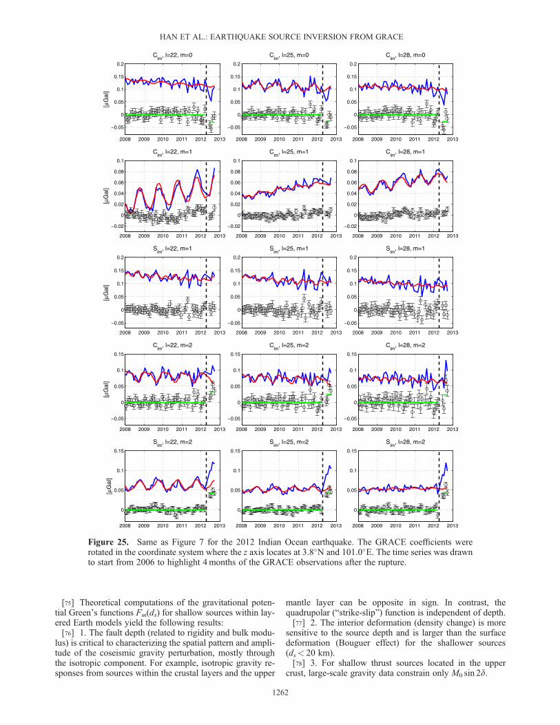
where t is the time elapsed since the rupture, is used to elim-inate the effect of viscous mantle relaxation on a time scalesignificantly longer than that expected from a seismicsource, even allowing for slow coseismic components. Thelinear and quadratic components were not included in the re-gression because they are correlated with the postseismictrends; however, the coseismic step estimates are notaffected, regardless of whether the linear and quadratic com-ponents are included or not (by virtue of sufficiently longtime series). In the time series regression, we did not usethe data in 2012 to avoid any potential influence by thenearby 2012 strike-slip earthquakes.[50] Figure 7 shows the time series of the GRACE L2 co-
efficients, localized within the domain shown in Figure 6a.The localized coefficient at degree l is computed with theneighboring coefficients, and thus creates correlation amongthe localized coefficients over degree (but independent overorder), effectively reducing random noise in the original L2data. For example, the localized coefficient at degree 30 wasinfluenced by the original GRACE coefficients at degrees 10to 50, because we used the windowing function expandedwith the maximum degree 20 (Lh = 20). The (localized) coef-ficients were plotted in the (epicentral) coordinate systemwhere the z axis locates at the center of the spatial windowfunction (5.4�N, 93.8�E). It is the location where the largestmoment was released according to the finite fault modelused in Han et al. [2006]. In this rotated coordinate system,the gravity coefficients at orders 0, 1, and 2 are directlyrelated to the moment tensor components of the centroid atthe pole (i.e., 5.4�N, 93.8�E in a geographic coordinatesystem), as described in equation (6). Almost all coefficientsbetween degrees 21 and 40 present large perturbations dueto the earthquake in episodic change as well as gradualchange afterwards. Although postseismic observations lastlong (>7 years), they need to be carefully examined sincethey might be affected by background gravity changes dueto inter-annual climate variability. The longer postseismictime series reveal that they may be better modeled with alogarithmic function than the exponential function used inHan et al. [2008] for the analysis of only 2.5 years ofpostseismic data. The coseismic SNR is found highest fromthe coefficients of Cl,1, Sl,1, and Sl,2, for Mrθ, Mrf, and Mθf,
respectively, and degrades forCl,2 andCl,0, related to the diag-onal components of the moment tensor, Mrr and Mθθ�Mff,respectively.[51] The coseismic step and its error estimates for each of
the localized coefficients were used for (linear) inversion ofthe moment tensor components m̂ and its covariance matrix,
C m̂n o
. From the condition Mrr+Mθθ +Mff = 0, we found
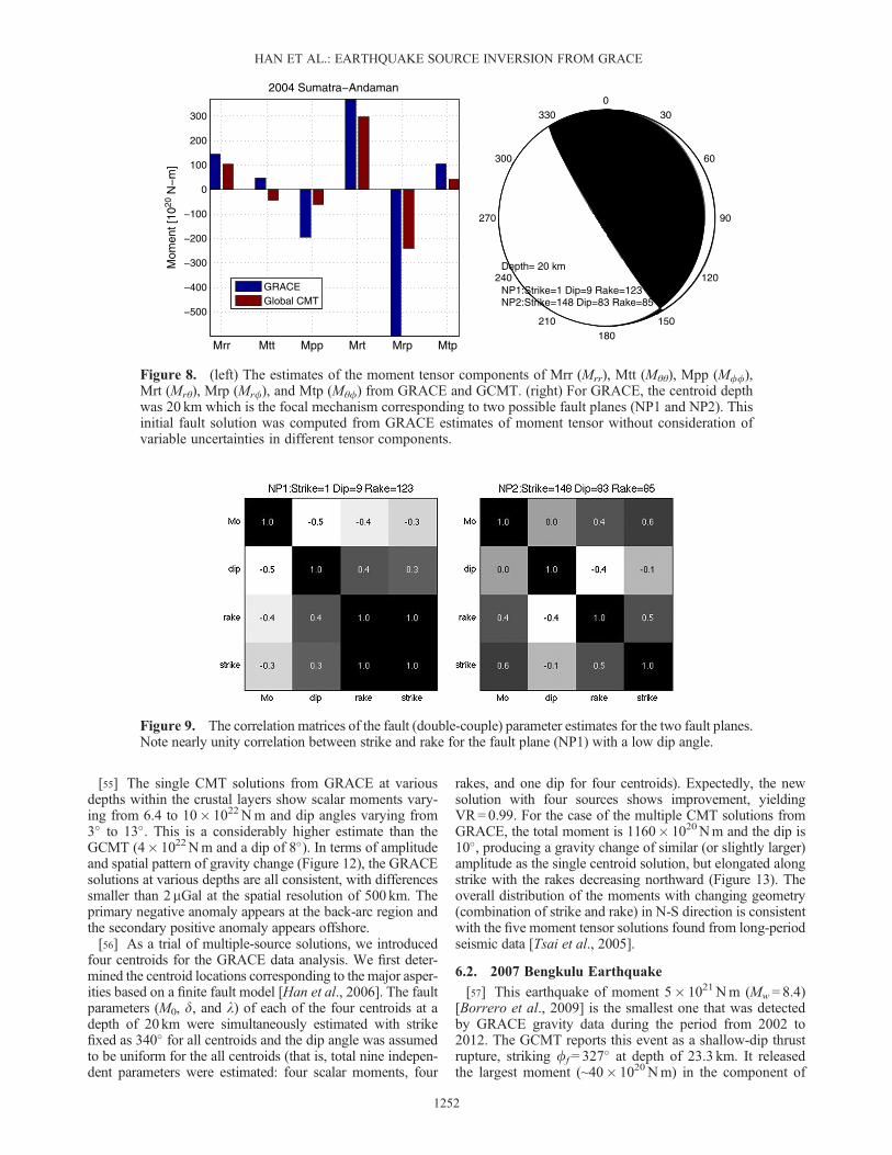
three diagonal components. The GRACE estimates at depthof 20 km and GCMT are compared in Figure 8, indicatingthat GCMT provides smaller estimates of the components,particularly Mrf. The corresponding focal mechanism dia-gram (i.e., “beachball”) was drawn by finding two faultplanes using the program mentioned in Section 5.1. Weuse them only as initial solutions for our inversion of thedouble-couple parameters reflecting the error characteristicsof the moment tensor estimates from GRACE.[52] First of all, the correlation matrix as discussed in
Section 5.2 was computed for both fault-plane solutions andshown in Figure 9. As suspected from the low dip fault plane,rake and strike are tightly coupled with nearly unity correla-tion, while the other fault plane solution does not yield suchstrong coupling between them. This pair of correlation charac-teristics is typical for other thrust events considered in thisstudy (note, however, that the correlation matrix looks differ-ent for the strike-slip event that will be discussed later).[53] Due to strong correlation between strike and rake, we
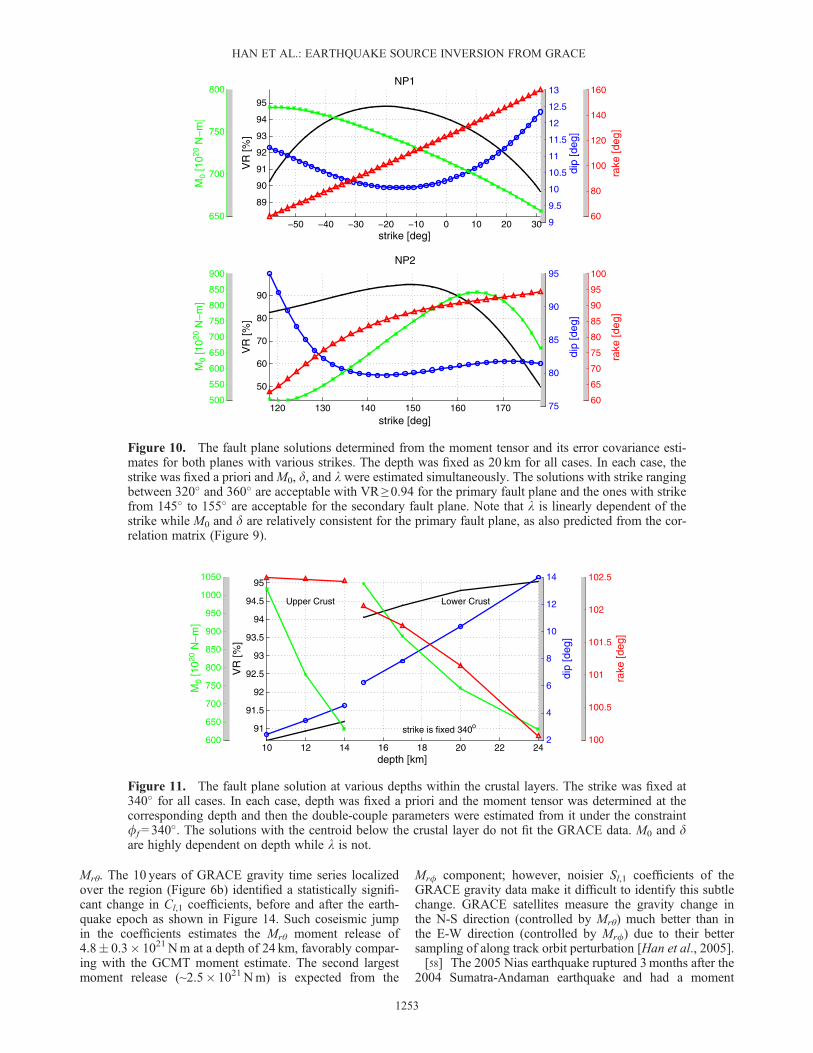
fixed strike ff a priori and solved for M0, d, and l simulta-neously from the moment tensor and its covariance estimatesfollowing the procedure in Section 5.2. The convergencewas always obtained within not more than three iterations.The solutions at various strikes for both fault planes areshown in Figure 10. By changing ff in 1� steps around theinitial strike, we found that double-couple solutions for theprimary fault plane with 320� ≤ff ≤ 360� fit equally wellthe GRACE observations. The rake parameter changes line-arly with strike, while the other parameters of M0 and d arerelatively constant. The trade-off between strike and rake isonly found for the plane with low dip angle. For the conju-gate fault plane, the secondary double-couple solution canbe delineated with ff = 150� � 5�, M0 ~ 750� 1020Nm,d ~ 82�, and l ~ 88�.[54] We tested sensitivity of the fault solutions to depth. In
this case, we fixed the strike at 340� and changed depthswithin the lower and upper crust and upper mantle (i.e., from10 to 30 km). The solutions in the crustal layers yielded var-iance reduction (VR) = 0.91–0.95, while for solutions in theupper mantle (not shown), VR= 0.70–0.75 was substantiallylower (Figure 11). Any solution within the crustal layer fitGRACE observations equally well with the ones in thelower crustal layer being even better. With increasingdepths, d gradually increases, while M0 decreases and l ispractically unchanged. The solutions at shallower depths,particularly within the upper crust, show larger changes inM0 with the variation in d or depth than do the deepersources, as expressed by a steeper slope in the ds�M0 ord�M0 plot in Figure 11. This indicates thatM0 is not robustlyresolved for the upper crustal solutions. As expected, forshallow thrust earthquakes, M0 sin 2d is better-constrained[Kanamori and Given, 1981; Tsai et al., 2011]. As depthincreases (i.e., lower crust), however, the effect becomes lessacute, and the resolution of M0 and d improves.
HAN ET AL.: EARTHQUAKE SOURCE INVERSION FROM GRACE
1250
2002 2004 2006 2008 2010 2012
−0.05
0
0.05
0.1
0.15
0.2
Clm, l=23, m=1
Clm, l=23, m=0
Clm, l=30, m=1 Clm, l=37, m=1
Slm, l=23, m=1 Slm, l=30, m=1 Slm, l=37, m=1
Slm, l=23, m=2 Slm, l=30, m=2 Slm, l=37, m=2
Clm, l=23, m=2 Clm, l=30, m=2 Clm, l=37, m=2
2002 2004 2006 2008 2010 2012
0
0.05
0.1
[µG
al]
[µG
al]
[µG
al]
[µG
al]
[µG
al]
2002 2004 2006 2008 2010 2012−0.2
−0.1
0
0.1
0.2
2002 2004 2006 2008 2010 2012
−0.05
0
0.05
0.1
0.15
0.2
0.25
2002 2004 2006 2008 2010 2012
0
0.05
0.1
0.15
2002 2004 2006 2008 2010 2012
−0.05
0
0.05
0.1
0.15
0.2
2002 2004 2006 2008 2010 2012
0
0.05
0.1
2002 2004 2006 2008 2010 2012−0.2
−0.1
0
0.1
0.2
2002 2004 2006 2008 2010 2012
−0.05
0
0.05
0.1
0.15
0.2
0.25
2002 2004 2006 2008 2010 2012
0
0.05
0.1
0.15
2002 2004 2006 2008 2010 2012
−0.05
0
0.05
0.1
0.15
0.2
2002 2004 2006 2008 2010 2012
0
0.05
0.1
2002 2004 2006 2008 2010 2012−0.2
−0.1
0
0.1
0.2
2002 2004 2006 2008 2010 2012
−0.05
0
0.05
0.1
0.15
0.2
0.25
2002 2004 2006 2008 2010 2012
0
0.05
0.1
0.15
Clm, l=37, m=0Clm, l=30, m=0
Figure 7. Monthly time series of the GRACE L2 data after applying the spatial localization over theSumatra-Andaman earthquake region (solid blue line) and the seasonal and inter-seasonal fit (solid redline). Arbitrary offsets were added for clarity. The data residual (black line with error bars) was computedby subtracting the fit (red line) from the data (blue line). The associated error bar was estimated from the fitobtained between 2002 and 2011. The data residuals were subsequently analyzed using the Heaviside stepand logarithmic functions for delineation of coseismic and postseismic changes, respectively (solid greenline). The GRACE coefficients were rotated to the epicentral coordinate system where the z axis locates at5.4�N and 93.8�E and the five lowest order (m= 0, 1, and 2; for both Clm and Slm) coefficients are shown atdifferent degrees between 21 and 40. From the top to bottom, these coefficients related to the momenttensor components, Mrr, Mrθ, Mrf, Mθθ�Mff, and Mθf, respectively.
HAN ET AL.: EARTHQUAKE SOURCE INVERSION FROM GRACE
1251
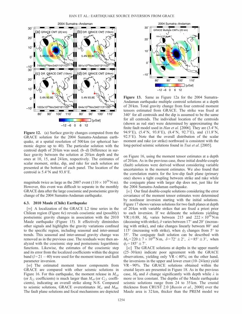
[55] The single CMT solutions from GRACE at variousdepths within the crustal layers show scalar moments vary-ing from 6.4 to 10� 1022Nm and dip angles varying from3� to 13�. This is a considerably higher estimate than theGCMT (4� 1022Nm and a dip of 8�). In terms of amplitudeand spatial pattern of gravity change (Figure 12), the GRACEsolutions at various depths are all consistent, with differencessmaller than 2mGal at the spatial resolution of 500 km. Theprimary negative anomaly appears at the back-arc region andthe secondary positive anomaly appears offshore.[56] As a trial of multiple-source solutions, we introduced
four centroids for the GRACE data analysis. We first deter-mined the centroid locations corresponding to the major asper-ities based on a finite fault model [Han et al., 2006]. The faultparameters (M0, d, and l) of each of the four centroids at adepth of 20 km were simultaneously estimated with strikefixed as 340� for all centroids and the dip angle was assumedto be uniform for the all centroids (that is, total nine indepen-dent parameters were estimated: four scalar moments, four
rakes, and one dip for four centroids). Expectedly, the newsolution with four sources shows improvement, yieldingVR=0.99. For the case of the multiple CMT solutions fromGRACE, the total moment is 1160� 1020Nm and the dip is10�, producing a gravity change of similar (or slightly larger)amplitude as the single centroid solution, but elongated alongstrike with the rakes decreasing northward (Figure 13). Theoverall distribution of the moments with changing geometry(combination of strike and rake) in N-S direction is consistentwith the five moment tensor solutions found from long-periodseismic data [Tsai et al., 2005].
6.2. 2007 Bengkulu Earthquake
[57] This earthquake of moment 5� 1021Nm (Mw = 8.4)[Borrero et al., 2009] is the smallest one that was detectedby GRACE gravity data during the period from 2002 to2012. The GCMT reports this event as a shallow-dip thrustrupture, striking ff= 327� at depth of 23.3 km. It releasedthe largest moment (~40� 1020Nm) in the component of
Figure 8. (left) The estimates of the moment tensor components of Mrr (Mrr), Mtt (Mθθ), Mpp (Mff),Mrt (Mrθ), Mrp (Mrf), and Mtp (Mθf) from GRACE and GCMT. (right) For GRACE, the centroid depthwas 20 km which is the focal mechanism corresponding to two possible fault planes (NP1 and NP2). Thisinitial fault solution was computed from GRACE estimates of moment tensor without consideration ofvariable uncertainties in different tensor components.
Figure 9. The correlation matrices of the fault (double-couple) parameter estimates for the two fault planes.Note nearly unity correlation between strike and rake for the fault plane (NP1) with a low dip angle.
HAN ET AL.: EARTHQUAKE SOURCE INVERSION FROM GRACE
1252
Mrθ. The 10 years of GRACE gravity time series localizedover the region (Figure 6b) identified a statistically signifi-cant change in Cl,1 coefficients, before and after the earth-quake epoch as shown in Figure 14. Such coseismic jumpin the coefficients estimates the Mrθ moment release of4.8� 0.3� 1021Nm at a depth of 24 km, favorably compar-ing with the GCMT moment estimate. The second largestmoment release (~2.5� 1021Nm) is expected from the
Mrf component; however, noisier Sl,1 coefficients of theGRACE gravity data make it difficult to identify this subtlechange. GRACE satellites measure the gravity change inthe N-S direction (controlled by Mrθ) much better than inthe E-W direction (controlled by Mrf) due to their bettersampling of along track orbit perturbation [Han et al., 2005].[58] The 2005 Nias earthquake ruptured 3months after the
2004 Sumatra-Andaman earthquake and had a moment
9
9.5
10
10.5
11
11.5
12
12.5
13
dip
[deg
]
650
700
750
800
60
80
100
120
140
160
rake
[deg
]
−50 −40 −30 −20 −10 0 10 20 30
89
90
91
92
93
94
95
strike [deg]V
R [%
]
NP1
75
80
85
90
95
dip
[deg
]
500
550
600
650
700
750
800
850
900
60
65
70
75
80
85
90
95
100
rake
[deg
]
120 130 140 150 160 170
50
60
70
80
90
strike [deg]
VR
[%]
NP2
M0
[1020
N−
m]
M0
[1020
N−
m]
Figure 10. The fault plane solutions determined from the moment tensor and its error covariance esti-mates for both planes with various strikes. The depth was fixed as 20 km for all cases. In each case, thestrike was fixed a priori andM0, d, and l were estimated simultaneously. The solutions with strike rangingbetween 320� and 360� are acceptable with VR ≥ 0.94 for the primary fault plane and the ones with strikefrom 145� to 155� are acceptable for the secondary fault plane. Note that l is linearly dependent of thestrike while M0 and d are relatively consistent for the primary fault plane, as also predicted from the cor-relation matrix (Figure 9).
2
4
6
8
10
12
14di
p [d
eg]
600
650
700
750
800
850
900
950
1000
1050
100
100.5
101
101.5
102
102.5
rake
[deg
]
10 12 14 16 18 20 22 24
91
91.5
92
92.5
93
93.5
94
94.5
95
depth [km]
VR
[%]
strike is fixed 340o
Upper Crust Lower Crust
M0
[1020
N−
m]
Figure 11. The fault plane solution at various depths within the crustal layers. The strike was fixed at340� for all cases. In each case, depth was fixed a priori and the moment tensor was determined at thecorresponding depth and then the double-couple parameters were estimated from it under the constraintff= 340�. The solutions with the centroid below the crustal layer do not fit the GRACE data. M0 and dare highly dependent on depth while l is not.
HAN ET AL.: EARTHQUAKE SOURCE INVERSION FROM GRACE
1253
magnitude twice as large as the 2007 event (110� 1020Nm).However, this event was difficult to separate in the monthlyGRACE data after the large coseismic and postseismic gravitychange of the 2004 Sumatra-Andaman earthquake.
6.3. 2010 Maule (Chile) Earthquake
[59] A localization of the GRACE L2 time series in theChilean region (Figure 6c) reveals coseismic and (possibly)postseismic gravity changes in association with the 2010Maule earthquake (Figure 15). It effectively diminishesother signals and highlights the gravity variations confinedto the specific region, including seasonal and inter-annualtrends. This seasonal and inter-annual gravity change wasremoved as in the previous case. The residuals were then an-alyzed with the coseismic step and postseismic logarithmicfunctions. Likewise, the estimates of the coseismic stepand its error from the localized coefficients within the degreeband (l= 21� 40) were used for the moment tensor and faultparameter inversion.[60] The estimated moment tensor components from
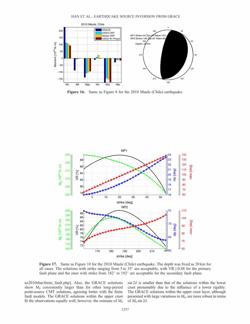
GRACE are compared with other seismic solutions inFigure 16. For this earthquake, the moment release in Mrf(or Sl,1 coefficients) is much larger than Mrθ (or Cl,1 coeffi-cients), indicating an overall strike along N-S. Comparedto seismic solutions, GRACE overestimates Mrr and Mθθ.The fault plane solutions and focal mechanisms are depicted
on Figure 16, using the moment tensor estimates at a depthof 20 km. As in the previous case, these initial double-couple(fault) solutions were derived without considering variableuncertainties in the moment estimates. We also found thatthe correlation matrix for the low-dip fault plane (primaryone) shows a tight coupling between strike and rake whilethe conjugate plane with larger dip does not, just like forthe 2004 Sumatra-Andaman earthquake.[61] Our final double-couple solutions considering the error
covariance of the moment tensor estimates were determinedby nonlinear inversion starting with the initial solutions.Figure 17 shows various solutions for two fault planes at depthof 20 km with variable strikes that are fixed a priori priorto each inversion. If we delineate the solutions yieldingVR≥ 0.88, M0 varies between 215 and 222� 1020Nm(deceasing with strike), d varies between 17� and 20� (increas-ing with strike), and rake changes linearly between 80� and115� (increasing with strike), when ff changes from 5� to35�. The conjugate fault solution can be described withM0 = 220� 7� 1020Nm, d =72� � 2�, l =85� � 3�, whenff=185� � 7�.[62] The GRACE solutions at depths in the upper mantle
(25–30 km) indicate poor agreement with the GRACEobservations, yielding only VR< 40%; on the other hand,the inversions in the upper and lower crust (10–24 km) yieldVR~ 90%. The GRACE solutions obtained within thecrustal layers are presented in Figure 18. As in the previouscase, M0 and d change significantly with depth while l ismore or less constant. The depths of the Maule earthquakeseismic solutions range from 24 to 35 km. The crustalthickness from CRUST 2.0 [Bassin et al., 2000] over theMaule area is 32 km, thicker than the PREM model we
(a) (b)
(d)(c)
Figure 12. (a) Surface gravity changes computed from theGRACE solution for the 2004 Sumatra-Andaman earth-quake, at a spatial resolution of 500 km (or spherical har-monic degree up to 40). The particular solution with thecentroid depth of 20 km was used. (b–d) Difference in sur-face gravity between the solution at 20 km depth and theones at 10, 15, and 24 km, respectively. The estimates ofscalar moment, strike, dip, and rake for each solution arepresented at the bottom of each panel. The location of thecentroid is 5.4�N and 93.8�E.
Figure 13. Same as Figure 12a for the 2004 Sumatra-Andaman earthquake multiple centroid solutions at a depthof 20 km. Total gravity change from four centroid momenttensors estimated from GRACE. The strike was fixed at340� for all centroids and the dip is assumed to be the samefor all centroids. The individual location of the centroids(shown as red star) were determined by approximating thefinite fault model used in Han et al. [2006]. They are (3.4�N,94.9�E), (5.4�N, 93.8�E), (8.4�N, 92.7�E), and (11.8�N,92.5�E). Note that the overall distribution of the scalarmoment and rake (or strike) northward is consistent with thelong-period seismic solutions found in Tsai et al. [2005].
HAN ET AL.: EARTHQUAKE SOURCE INVERSION FROM GRACE
1254
used. Therefore, the GRACE solutions at the lower boundof the lower crust would be preferable. This particular
solution is also consistent with most of other solutions interms of the dip angle and moment [Lay et al., 2010;
Figure 14. Same as Figure 7 for the 2007 Bengkulu earthquake. Note that the Cl,1 coefficients present asignificant step before and after the epoch of the event in 2007. This particular earthquake was strongest inthe component of Mrθ.
HAN ET AL.: EARTHQUAKE SOURCE INVERSION FROM GRACE
1255
G Shao et al., Preliminary Slip Model of the Feb 27, 2010Mw 8.9Maule, Chile Earthquake, 2010, http://www.geol.ucsb.edu/faculty/ji/big_earthquakes/2010/02/27/chile_2_27.html;
G. P. Hayes 2010, Finite Fault Model, Updated Result ofthe Feb 27, 2010 Mw 8.8 Maule, Chile Earthquake,http://earthquake.usgs.gov/earthquakes/eqinthenews/2010/
Figure 15. Same as Figure 7 for the 2010 Maule (Chile) earthquake. The GRACE coefficients were ro-tated in the coordinate system where the z axis locates at 35.6�S and 286.9�E.
HAN ET AL.: EARTHQUAKE SOURCE INVERSION FROM GRACE
us2010tfan/finite_fault.php]. Also, the GRACE solutionsshow M0 consistently larger than for other long-periodpoint-source CMT solutions, agreeing better with the finitefault models. The GRACE solutions within the upper crustfit the observations equally well; however, the estimate ofM0
sin 2d is smaller than that of the solutions within the lowercrust presumably due to the influence of a lower rigidity.The GRACE solutions within the upper crust layer, althoughpresented with large variations inM0, are more robust in termsof M0 sin 2d.
Figure 16. Same as Figure 8 for the 2010 Maule (Chile) earthquake.
16
17
18
19
20
21
22
23
24
dip
[deg
]
200
205
210
215
220
225
M0
[1020
N−
m]
M0
[1020
N−
m]
60
70
80
90
100
110
120
130
140
rake
[deg
]
0 10 20 30 40 5078
80
82
84
86
88
strike [deg]
VR
[%]
NP1
60
65
70
75
dip
[deg
]
160
170
180
190
200
210
220
230
240
60
70
80
90
100
110
rake
[deg
]
170 180 190 200 210 220
727476788082848688
strike [deg]
VR
[%]
NP2
Figure 17. Same as Figure 10 for the 2010 Maule (Chile) earthquake. The depth was fixed as 20 km forall cases. The solutions with strike ranging from 5 to 35� are acceptable, with VR ≥ 0.88 for the primaryfault plane and the ones with strike from 182� to 192� are acceptable for the secondary fault plane.
HAN ET AL.: EARTHQUAKE SOURCE INVERSION FROM GRACE
[63] The gravity change was computed using the GRACECMT solution at a depth of 24 km (Figure 19). It shows,likewise, the primary, negative, anomaly on land (back-arcregion) and secondary, positive, anomaly offshore. Thedifferences in terms of gravity (at 500 km resolution) amongthe solutions at depths of 10, 15, and 20 km are less than1 mGal, while the dip angle estimates vary from 6 to 24ºand the moment estimates from 207 to 276� 1020Nm,depending on depth.[64] For this event, we note that the lateral surface density
heterogeneity due to the South American continent (beingdifferent from the uniform ocean layer used in our calcula-tion) might be important. We made some ad hoc computa-tions to roughly quantify the effect of land by combiningthe ocean anomaly computed with the uniform ocean layerand the land anomaly computed without the ocean layer.The eigenfunctions were computed using two different 1DEarth models with and without the ocean layer. We found
the lateral heterogeneity may cause a difference in thenegative gravity on land by 2 mGal at maximum. We defermore reasonable assessment of the surface heterogeneityin gravity to the computation of eigenfunctions with a 3DEarth model and sea level equation such as in Broerseet al. [2011].
6.4. 2011 Tohoku-Oki (Japan) Earthquake
[65] Figure 20 presents the time series of the sameGRACE L2 coefficients, but localized around the areashown in Figure 6d, at m= 0, 1, and 2 and the regression fits.After removing the mean, linear, and quadratic polynomialsand annual and semi-annual sinusoids, the residual data areanalyzed for the coseismic and postseismic changes. All fivemoment tensor components present significant coseismicand postseismic signature in the time series. Compared tothe time series around the Maule earthquake, this area isaffected less by systematic variations in gravity.[66] The coseismic step and its error estimates for each of
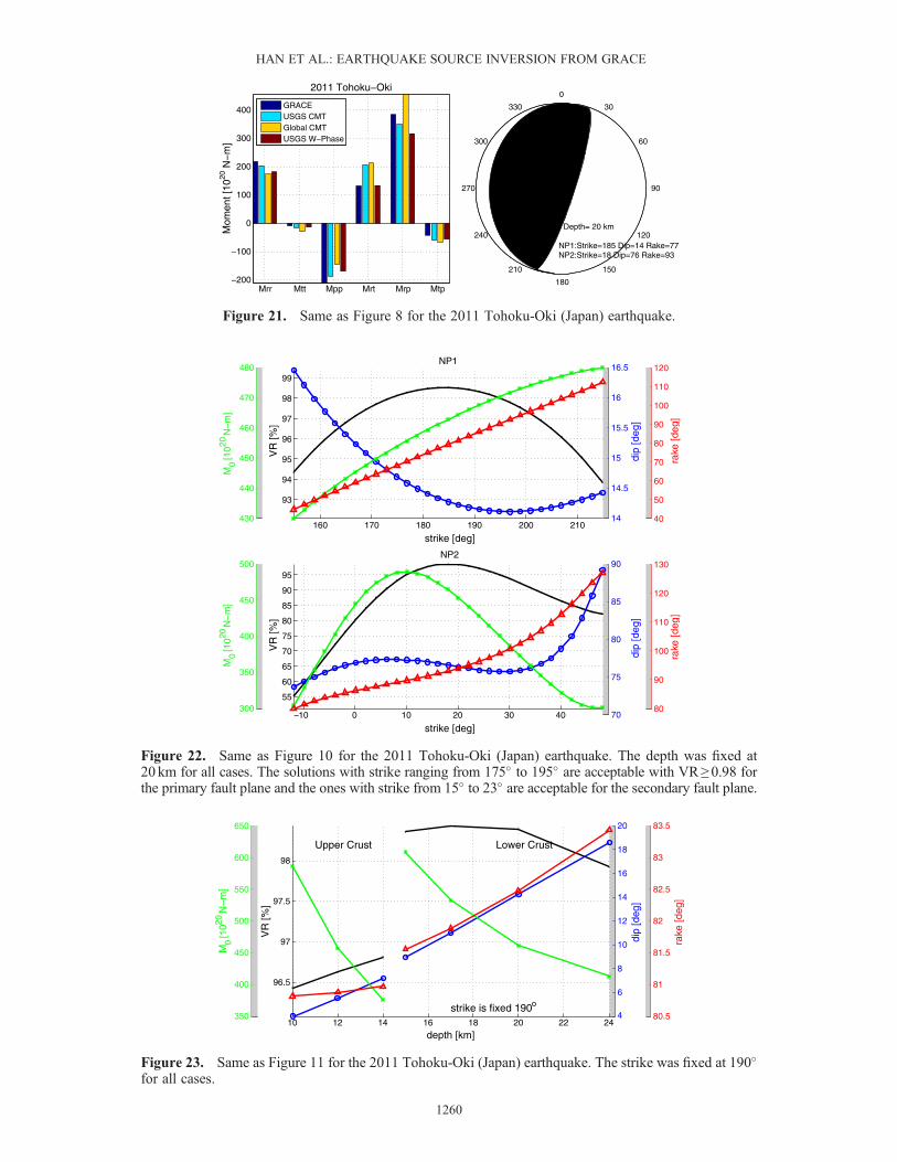
the localized coefficients were used for inversion of themoment tensor components at various depths. The solutionsat 20 km are shown in Figure 21 along with other seismicsolutions. The focal mechanism parameters were obtainedfor the primary and conjugate fault planes as also shown inFigure 21. All moment tensor components from GRACE at20 km are in good agreement with seismic solutions. Onceagain, the fault plane solution with low dip angle yields nearlyunity correlation between rake and strike, while it is notthe case for the other fault plane. Therefore, we fix thestrike a priori to obtain the double-couple solutions, andthen test various strikes (Figure 22). Solutions featuringM0 = 450–470� 1020Nm (increasing with strike), d =14�–5�(decreasing with strike), l changing linearly from 65� to 90�(increasing with strike), and ff=175�–95� all fit the GRACEobservations equally well, withVR≥ 98%. The conjugate faultsolution can be described with M0 = 450� 20� 1020Nm,d =77� � 1�, l=95� � 3�, when ff=18� � 3�.[67] The solutions with the centroid in the upper mantle
(depth greater than 24 km in PREM) indicated consistentlypoorer agreement with the GRACE observations, yieldingVR� 50%, compared to the ones within the upper and lowercrust with VR> 90%. Therefore, we ruled out the solutionswithin the upper mantle and only show in Figure 23 theother solutions located within the crustal layers. The uppercrustal solutions show dip angles of 7� and less and scalarmoments of 380–600� 1020Nm. The solutions within thelower crust indicate a dip ranging from 9� to 19� and M0
6
8
10
12
14
16
18
20
22
24
dip
[deg
]
180
190
200
210
220
230
240
250
260
270
280
M0
[1020
N−
m]
102
102.5
103
103.5
104
104.5
105
105.5
106
106.5
rake
[deg
]
10 12 14 16 18 20 22 24
88.4
88.6
88.8
89
89.2
89.4
89.6
89.8
depth [km]V
R [%
]
strike is fixed 19o
Upper Crust Lower Crust
Figure 18. Same as Figure 11 for the 2010Maule (Chile) earthquake. The strike was fixed at 19� for all cases.
Figure 19. Same as Figure 12 for the 2010 Maule (Chile)earthquake. The location of the centroid is 35.6�S and286.9�E.
HAN ET AL.: EARTHQUAKE SOURCE INVERSION FROM GRACE
1258
ranging 410 to 620� 1020Nm, depending on the precisedepth. In both cases, the shallower the depth in each layer,the smaller the dip and the larger the moment. When com-pared with other seismic and GPS-based solutions includinglong-period CMT and the moment-weighted CMT from var-ious finite fault models [Shao et al., 2011; Simons et al.,2011; Hayes, 2011; Ammon et al., 2011], only the GRACEsolutions within the lower crust are consistent with those
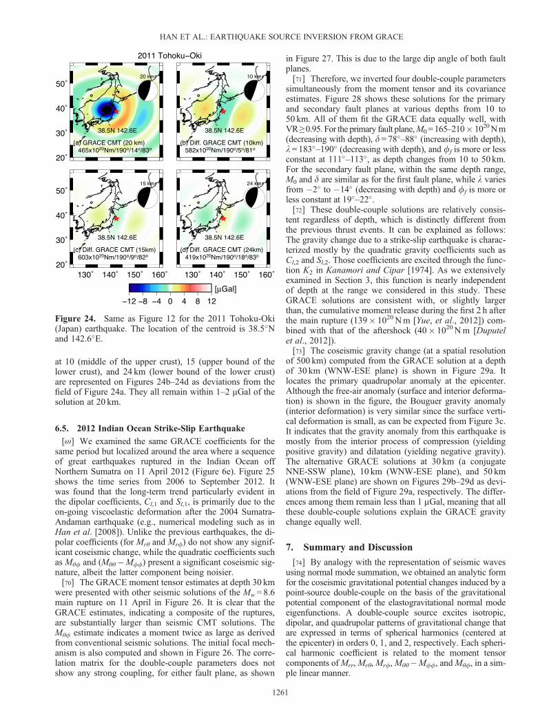
alternative solutions in moment and dip, as well as depth(except for the USGS CMT in depth).[68] The coseismic gravity change (at a spatial resolution
of 500 km), computed from the GRACE solution for a depthof 20 km, is shown in Figure 24a. It locates the primary neg-ative anomaly in the back-arc region and the secondary pos-itive anomaly (with one third the amplitude of the primaryanomaly) near the trench. The alternative GRACE solutions
2002 2004 2006 2008 2010 2012
−0.05
0
0.05
0.1
[µG
al]
Clm
, l=23, m=0
2002 2004 2006 2008 2010 2012−0.05
0
0.05
0.1
[µG
al]
Clm
, l=23, m=1
2002 2004 2006 2008 2010 2012−0.2
−0.1
0
0.1
0.2
[µG
al]
Slm
, l=23, m=1
2002 2004 2006 2008 2010 2012−0.1
−0.05
0
0.05
0.1
0.15
0.2
[µG
al]
Clm
, l=23, m=2
2002 2004 2006 2008 2010 2012−0.05
0
0.05
0.1
[µG
al]
Slm
, l=23, m=2
2002 2004 2006 2008 2010 2012
−0.05
0
0.05
0.1
Clm
, l=30, m=0
2002 2004 2006 2008 2010 2012−0.05
0
0.05
0.1
Clm
, l=30, m=1
2002 2004 2006 2008 2010 2012−0.2
−0.1
0
0.1
0.2
Slm
, l=30, m=1
2002 2004 2006 2008 2010 2012−0.1
−0.05
0
0.05
0.1
0.15
0.2
Clm
, l=30, m=2
2002 2004 2006 2008 2010 2012−0.05
0
0.05
0.1
Slm
, l=30, m=2
2002 2004 2006 2008 2010 2012
−0.05
0
0.05
0.1
Clm
, l=37, m=0
2002 2004 2006 2008 2010 2012−0.05
0
0.05
0.1
Clm
, l=37, m=1
2002 2004 2006 2008 2010 2012−0.2
−0.1
0
0.1
0.2
Slm
, l=37, m=1
2002 2004 2006 2008 2010 2012−0.1
−0.05
0
0.05
0.1
0.15
0.2
Clm
, l=37, m=2
2002 2004 2006 2008 2010 2012−0.05
0
0.05
0.1
Slm
, l=37, m=2
Figure 20. Same as Figure 7 for the 2011 Tohoku-Oki (Japan) earthquake. The GRACE coefficientswere rotated in the coordinate system where the z axis locates at 38.5�N and 142.6�E. Higher noise in2002 is due to the use of RL04 GRACE products. The quality of the product is improved with RL05 asshown in the rest of the years.
HAN ET AL.: EARTHQUAKE SOURCE INVERSION FROM GRACE
Figure 21. Same as Figure 8 for the 2011 Tohoku-Oki (Japan) earthquake.
14
14.5
15
15.5
16
16.5
dip
[deg
]
430
440
450
460
470
480
M0 [1
020 N
−m
]
40
50
60
70
80
90
100
110
120
rake
[deg
]
160 170 180 190 200 210
93
94
95
96
97
98
99
strike [deg]
VR
[%]
NP1
70
75
80
85
90
dip
[deg
]
300
350
400
450
500
M0 [1
020N
−m
]
80
90
100
110
120
130
rake
[deg
]
−10 0 10 20 30 40
55
60
65
70
75
80
85
90
95
strike [deg]
VR
[%]
NP2
Figure 22. Same as Figure 10 for the 2011 Tohoku-Oki (Japan) earthquake. The depth was fixed at20 km for all cases. The solutions with strike ranging from 175� to 195� are acceptable with VR≥ 0.98 forthe primary fault plane and the ones with strike from 15� to 23� are acceptable for the secondary fault plane.
4
6
8
10
12
14
16
18
20
dip
[deg
]
350
400
450
500
550
600
650
M0 [1
020 N
−m
]
80.5
81
81.5
82
82.5
83
83.5
rake
[deg
]
10 12 14 16 18 20 22 24
96.5
97
97.5
98
depth [km]
VR
[%]
strike is fixed 190o
Upper Crust Lower Crust
Figure 23. Same as Figure 11 for the 2011 Tohoku-Oki (Japan) earthquake. The strike was fixed at 190�for all cases.
HAN ET AL.: EARTHQUAKE SOURCE INVERSION FROM GRACE
1260
at 10 (middle of the upper crust), 15 (upper bound of thelower crust), and 24 km (lower bound of the lower crust)are represented on Figures 24b–24d as deviations from thefield of Figure 24a. They all remain within 1–2 mGal of thesolution at 20 km.
6.5. 2012 Indian Ocean Strike-Slip Earthquake
[69] We examined the same GRACE coefficients for thesame period but localized around the area where a sequenceof great earthquakes ruptured in the Indian Ocean offNorthern Sumatra on 11 April 2012 (Figure 6e). Figure 25shows the time series from 2006 to September 2012. Itwas found that the long-term trend particularly evident inthe dipolar coefficients, Cl,1 and Sl,1, is primarily due to theon-going viscoelastic deformation after the 2004 Sumatra-Andaman earthquake (e.g., numerical modeling such as inHan et al. [2008]). Unlike the previous earthquakes, the di-polar coefficients (for Mrθ and Mrf) do not show any signif-icant coseismic change, while the quadratic coefficients suchas Mθf and (Mθθ�Mff) present a significant coseismic sig-nature, albeit the latter component being noisier.[70] The GRACE moment tensor estimates at depth 30 km
were presented with other seismic solutions of the Mw = 8.6main rupture on 11 April in Figure 26. It is clear that theGRACE estimates, indicating a composite of the ruptures,are substantially larger than seismic CMT solutions. TheMθf estimate indicates a moment twice as large as derivedfrom conventional seismic solutions. The initial focal mech-anism is also computed and shown in Figure 26. The corre-lation matrix for the double-couple parameters does notshow any strong coupling, for either fault plane, as shown
in Figure 27. This is due to the large dip angle of both faultplanes.[71] Therefore, we inverted four double-couple parameters
simultaneously from the moment tensor and its covarianceestimates. Figure 28 shows these solutions for the primaryand secondary fault planes at various depths from 10 to50 km. All of them fit the GRACE data equally well, withVR≥0.95. For the primary fault plane,M0=165–210� 1020Nm(decreasing with depth), d =78�–88� (increasing with depth),l =183�–190� (decreasing with depth), and ff is more or lessconstant at 111�–113�, as depth changes from 10 to 50 km.For the secondary fault plane, within the same depth range,M0 and d are similar as for the first fault plane, while l variesfrom �2� to �14� (decreasing with depth) and ff is more orless constant at 19�–22�.[72] These double-couple solutions are relatively consis-
tent regardless of depth, which is distinctly different fromthe previous thrust events. It can be explained as follows:The gravity change due to a strike-slip earthquake is charac-terized mostly by the quadratic gravity coefficients such asCl,2 and Sl,2. Those coefficients are excited through the func-tion K2 in Kanamori and Cipar [1974]. As we extensivelyexamined in Section 3, this function is nearly independentof depth at the range we considered in this study. TheseGRACE solutions are consistent with, or slightly largerthan, the cumulative moment release during the first 2 h afterthe main rupture (139� 1020Nm [Yue, et al., 2012]) com-bined with that of the aftershock (40� 1020Nm [Duputelet al., 2012]).[73] The coseismic gravity change (at a spatial resolution
of 500 km) computed from the GRACE solution at a depthof 30 km (WNW-ESE plane) is shown in Figure 29a. Itlocates the primary quadrupolar anomaly at the epicenter.Although the free-air anomaly (surface and interior deforma-tion) is shown in the figure, the Bouguer gravity anomaly(interior deformation) is very similar since the surface verti-cal deformation is small, as can be expected from Figure 3c.It indicates that the gravity anomaly from this earthquake ismostly from the interior process of compression (yieldingpositive gravity) and dilatation (yielding negative gravity).The alternative GRACE solutions at 30 km (a conjugateNNE-SSW plane), 10 km (WNW-ESE plane), and 50 km(WNW-ESE plane) are shown on Figures 29b–29d as devi-ations from the field of Figure 29a, respectively. The differ-ences among them remain less than 1 mGal, meaning that allthese double-couple solutions explain the GRACE gravitychange equally well.
7. Summary and Discussion
[74] By analogy with the representation of seismic wavesusing normal mode summation, we obtained an analytic formfor the coseismic gravitational potential changes induced by apoint-source double-couple on the basis of the gravitationalpotential component of the elastogravitational normal modeeigenfunctions. A double-couple source excites isotropic,dipolar, and quadrupolar patterns of gravitational change thatare expressed in terms of spherical harmonics (centered atthe epicenter) in orders 0, 1, and 2, respectively. Each spheri-cal harmonic coefficient is related to the moment tensorcomponents ofMrr,Mrθ,Mrf,Mθθ�Mff, andMθf, in a sim-ple linear manner.
Figure 24. Same as Figure 12 for the 2011 Tohoku-Oki(Japan) earthquake. The location of the centroid is 38.5�Nand 142.6�E.
HAN ET AL.: EARTHQUAKE SOURCE INVERSION FROM GRACE
1261
[75] Theoretical computations of the gravitational poten-tial Green’s functions Fm(ds) for shallow sources within lay-ered Earth models yield the following results:[76] 1. The fault depth (related to rigidity and bulk modu-
lus) is critical to characterizing the spatial pattern and ampli-tude of the coseismic gravity perturbation, mostly throughthe isotropic component. For example, isotropic gravity re-sponses from sources within the crustal layers and the upper
mantle layer can be opposite in sign. In contrast, thequadrupolar (“strike-slip”) function is independent of depth.[77] 2. The interior deformation (density change) is more
sensitive to the source depth and is larger than the surfacedeformation (Bouguer effect) for the shallower sources(ds< 20 km).[78] 3. For shallow thrust sources located in the upper
crust, large-scale gravity data constrain only M0 sin 2d.
2008 2009 2010 2011 2012 2013
−0.05
0
0.05
0.1
0.15
0.2
[µG
al]
Clm
, l=22, m=0
2008 2009 2010 2011 2012 2013
−0.02
0
0.02
0.04
0.06
0.08
0.1
[µG
al]
Clm
, l=22, m=1
2008 2009 2010 2011 2012 2013
−0.05
0
0.05
0.1
0.15
0.2
[µG
al]
Slm
, l=22, m=1
2008 2009 2010 2011 2012 2013
−0.05
0
0.05
0.1
0.15
[µG
al]
Clm
, l=22, m=2
2008 2009 2010 2011 2012 2013
0
0.05
0.1
0.15
[µG
al]
Slm
, l=22, m=2
2008 2009 2010 2011 2012 2013
−0.05
0
0.05
0.1
0.15
0.2
Clm
, l=25, m=0
2008 2009 2010 2011 2012 2013
−0.02
0
0.02
0.04
0.06
0.08
0.1
Clm
, l=25, m=1
2008 2009 2010 2011 2012 2013
−0.05
0
0.05
0.1
0.15
0.2
Slm
, l=25, m=1
2008 2009 2010 2011 2012 2013
−0.05
0
0.05
0.1
0.15
Clm
, l=25, m=2
2008 2009 2010 2011 2012 2013
0
0.05
0.1
0.15
Slm
, l=25, m=2
2008 2009 2010 2011 2012 2013
−0.05
0
0.05
0.1
0.15
0.2
Clm
, l=28, m=0
2008 2009 2010 2011 2012 2013
−0.02
0
0.02
0.04
0.06
0.08
0.1
Clm
, l=28, m=1
2008 2009 2010 2011 2012 2013
−0.05
0
0.05
0.1
0.15
0.2
Slm
, l=28, m=1
2008 2009 2010 2011 2012 2013
−0.05
0
0.05
0.1
0.15
Clm
, l=28, m=2
2008 2009 2010 2011 2012 2013
0
0.05
0.1
0.15
Slm
, l=28, m=2
Figure 25. Same as Figure 7 for the 2012 Indian Ocean earthquake. The GRACE coefficients wererotated in the coordinate system where the z axis locates at 3.8�N and 101.0�E. The time series was drawnto start from 2006 to highlight 4months of the GRACE observations after the rupture.
HAN ET AL.: EARTHQUAKE SOURCE INVERSION FROM GRACE
1262
[79] 4. For low-dip thrust events, strike and rake aretightly coupled in a manner such that only their differenceis constrained.[80] All of these indicate that there might be trade-offs
among the source parameters: scalar moment and dip withfault depth and strike and rake when dip is small.[81] We developed an inversion method to estimate the
fault parameters from global gravitational potential observa-tions expressed as spherical harmonic coefficients, andapplied it to the 2004 Sumatra-Andaman, 2010Maule (Chile),2011 Tohoku-Oki (Japan), and 2012 Indian Ocean earth-quakes. A significant change in certain gravity coefficientsrelated to Mrθ was also observed after the 2007 Bengkuluearthquake. For the thrust events, we found that centroidsolutions within the upper and lower crust (ds< 25 km) giveconsiderably better fits to the GRACE data than the deeperones do located within the upper mantle (ds> 25 km). Weinterpret this result as due to an increase in bulk modulus(incompressibility) with depth responsible for the discordancein the resulting synthetics, as also found by Cambiotti et al.[2011]. In addition, crustal solutions (both upper and lower)yield more robust values of the parameterm�1
s M0 sin2d, wherems is the source rigidity, and thus of Δu sin 2d (where Δu is theseismic slip). Note that the latter is directly representative of
the vertical component of slip in the limit angles d for whichcos d is stationary. Other seismic and geodetic solutions areconsistent with the GRACE solutions within the lower crust.For the strike-slip events in 2012, the double-couple solutionspresent no significant depth-dependency and no trade-offamong the fault parameters.[82] In terms of spatial patterns of coseismic gravity
changes, the GRACE observations consistently found pri-mary negative gravity anomalies in the back-arc region andsmaller positive anomalies offshore, for the three thrustevents in 2004, 2010, and 2011. The negative anomaly orig-inates mostly from the isotropic term expressing the influ-ence of dilatation through the excitation function K0 ofKanamori and Cipar [1974]. The deeper sources, locatedwithin the upper mantle with larger bulk and rigidity modulithan in the crust, cannot reproduce the larger negative grav-ity changes. In this respect, the satellite gravity observationsfrom the megathrust events can be interpreted as expressinglarge-scale interior deformation associated with densitychanges (dilatation) inside the crustal layers. From thestrike-slip event in 2012, the gravity change is, again, mostlyfrom the interior process since the gravity effect from thevertical deformation at the crust-ocean interface is an orderof magnitude smaller. The quadrupolar gravity pattern,
Figure 26. Same as Figure 8 for the 2012 Indian Ocean earthquake. Note that GRACE indicates acumulative moment release from all events while various CMT solutions involve only the major event.
Figure 27. Same as Figure 9 for the 2012 Indian Ocean earthquake. Unlike the previous thrust eventscharacterized by a shallow-dipping fault plane, there is no tight coupling among the double-couple param-eters for both fault planes.
HAN ET AL.: EARTHQUAKE SOURCE INVERSION FROM GRACE
1263
being positive in ENE and WSW quadrants and negative inNNW and SSE quadrants, indicates compression and dilata-tion, respectively, radially inside the Earth.[83] Our work also offers the possibility of investigating
the presence of any ultraslow components in the spectrumof the seismic source. The largest ever earthquake recorded,the 1960 Chilean event was documented by Kanamori andCipar [1974], Kanamori and Anderson [1975] and Cifuentesand Silver [1989] to include a slow precursor, which started15min before the high-frequency rupture, and may have had acomparable moment. Similarly, a number of studies of the2004 Sumatra earthquake (including the modeling of its nor-mal modes) have shown that its very-long period moment,1.15� 1023Nm, was more than 2.5 times greater than thatderived from the standard GCMT algorithm, indicating anelement of slowness also expressed in other characteristics ofits source [Stein and Okal, 2005; Tsai et al., 2005; Choy andBoatwright, 2007]. Preliminary evidence also suggests thatthe 1964 Alaska earthquake, and possibly the Rat Island earth-quake of 1965, may have featured a similar component ofsource slowness [Nettles et al., 2005]. By contrast, the normalmodes of the 2010 Chilean and 2011 Tohoku events do notreveal any such slowness [Okal et al., 2012; Okal, 2012].[84] Because the inversion of GRACE L2 data uses
successive orbits for a month, the seismic moments resolvedin the present study represent averages over a time windowmuch longer than accessible from seismic data. The latter
are limited in principle by the period of the Earth’s gravestmode, 0S2 (3232 s), and in practice most classical CMT in-versions are carried at periods not exceeding 300 s. Conse-quently, the comparison between our results and classicalseismological ones can shed some light on the behavior ofthe source on time scales transgressing the seismic spectrum:a significant disparity between a GRACE moment and a(seismic) CMT solution would be a proxy for the existenceof a slow source component releasing moment at frequenciesbelow that of 0S2, while obviously it could not resolve thedetails of such a component (e.g., whether it was precursory,coseismic or took place 10 days after the main shock).[85] 1. For the 2004 Sumatra-Andaman earthquake, the
composite GRACE solution consisting of four sources elon-gated along strike yields a composite moment of 1.2� 1023
Nm with a dip of 10�, in excellent agreement with the valueof 1.2� 1023Nm obtained at ultralong seismic periods byTsai et al. [2005] and Okal and Stein [2009], and about2.5 to 3 times greater than the classical GCMT solution.We conclude that GRACE confirms the slow componentsoccasionally documented at frequencies lower than thoseof CMT inversions, but fails to unearth even slower ones,with characteristic times of hours to days, whose existencecould not have been a priori excluded.[86] 2. For the 2010 Maule, Chile earthquake, our solu-
tions range from 2.0 to 2.7� 1022Nm for dips between12� and 24�, and centroid depths between 15 and 24 km.
78
79
80
81
82
83
84
85
86
87
88
dip
[deg
]
160
165
170
175
180
185
190
195
200
205
210
M0 [1
020 N
−m
]
182
183
184
185
186
187
188
189
190
rake
[deg
]
10 15 20 25 30 35 40 45 50
110.6
110.8
111
111.2
111.4
111.6
111.8
112
112.2
112.4
112.6
depth [km]
strik
e [d
eg]
NP1
Mo, strike, dip and rake are estimated simultaneously
with consideration of error covariance of the moment tensor estimates
VR > 95%
80
81
82
83
84
85
86
87
88
dip
[deg
]
160
165
170
175
180
185
190
195
200
205
210
M0 [1
020 N
−m]
−15
−10
−5
0
rake
[deg
]
10 15 20 25 30 35 40 45 50
19
19.5
20
20.5
21
21.5
22
depth [km]
strik
e [d
eg]
NP2
VR > 95%
Figure 28. Same as Figure 11 for the 2012 Indian Ocean earthquake. In this earthquake, the simulta-neous solutions of the double-couple parameters were obtained at various depths for both fault planes(due to no tight coupling among the parameters). All the solutions produce VR ≥ 0.95. A distinct differ-ence from the previous thrust events is that the double-couple solutions of this strike-slip earthquakeare relatively consistent regardless of depths. The scalar moment estimate from GRACE is consistent withthe cumulative moment release from a series of the main ruptures and aftershocks.
HAN ET AL.: EARTHQUAKE SOURCE INVERSION FROM GRACE
1264
These numbers compare favorably with finite fault modelssuch as Lay et al.’s [2010] (M0= 2.1� 1022Nm), and areonly about 20% greater than the GCMT solution.[87] 3. In the case of the 2011 Tohoku-Oki earthquake,
scalar moments estimated from GRACE data range from4.1 to 6.1� 1022Nm, with dips between 9� and 19� anddepths between 15 and 24 km. This is in excellent agreementwith the published GCMT value (5.3� 1022Nm) and sup-ports Okal’s [2012] conclusion that the earthquake doesnot feature anomalous source slowness.[88] 4. For the 2012 Indian Ocean strike-slip earth-
quakes, GRACE estimates the scalar moment at 1.9 �1022Nm at a depth of 30 km, 60% larger than the com-bined GCMT values for the mainshock and aftershock(0.9� 1022Nm and 0.3� 1022Nm respectively), but com-paring favorably with the total moment of 1.4� 1022Nmof the finite fault solution of the main shock sequence byYue et al. [2012] combined with the estimate of 0.3� 1022Nm for the aftershock [Duputel et al., 2012].[89] 5. The detection of the 2007 Bengkulu earthquake
(M0= 50� 1020Nm; Mw= 8.5) may demonstrate the lowerbound for the use of GRACE gravity data to resolve earth-quake deformation. This was feasible due to the highest sen-sitivity of GRACE data to gravity change in N-S direction,where the spatial resolution could improve 400–500 km toas little as 200–300 km.[90] In this work, we attempted to characterize five great
earthquakes in terms of a centroid (point) representation,although the laterally and vertically distributed moments or
slips with a finite dimension of fault would be more suitablefor such large earthquakes. Our quantification of the centroidsources from gravity observations compares, in general, fa-vorably with other seismic centroid solutions. When jointlyanalyzed with other terrestrial data (like GPS and seismic re-cords), GRACE gravity data will provide seldom-observed,broad-scale constraints on the spatial distribution of slip.[91] The gradual postseismic changes over a time frame
of several years observed in most cases should not beoverlooked. Continuous observations of gravitational poten-tial changes will be useful to document the rheologicalresponse of the Earth to great earthquakes and to advanceour understanding of post-earthquake stress and strain redis-tribution. These data could provide, for example, an insightinto bulk behavior: time-dependent (inelastic) bulk modulus[Rundle, 1978; Rundle and Smith, 1982] versus no signifi-cant bulk relaxation [Cohen, 1980a, 1980b; Ivins andSammis, 1996; Pollitz, 1997]. These could be indispensablefor understanding the large-scale behavior of the Earth’sshallow material, and eventually for earthquake hazardassessment and mitigation applications. Finally, the futureGRACE follow-on mission equipped with enhanced instru-mentation [Watkins, 2011] may allow us to exploit gravita-tional potential data in the analysis of smaller, and thus morefrequent seismic events than the ones studied here. The tran-sient gravitational perturbations available from L1B orbitperturbation data could deliver additional understanding atthe seismic frequencies.
Appendix A: On the Behavior of Isotropic GravityResponse From Shallow Sources
[92] In order to investigate the isotropic gravity responsefunction F0(ds), we examine the excitation function nK0;l
given in Kanamori and Cipar [1974] using the eigenfunctioncomponents defined by Alterman et al. [1959]. This can be re-written by introducing the dilatation component as (we specifyhere the degree l and overtone n, explicitly):
nK0;ldsð Þ ¼ 2l þ 1
4pnsl2 I1 þ l l þ 1ð ÞI2½ � nX l dsð Þ � 3n _y1;l dsð Þ
n o; (A1)
where nsl is the eigenfrequency; nXl is the dilatation
eigenfunction that can be written as n X l ¼ n _y1;lþ 2
r n y1;l� l lþ1ð Þ
r n y3;l, and n _y1;l
is the radial derivative of n y1;l : n _y1;l ¼�2�l
�l þ 2mð Þr n y1;l þ1
�l þ 2mð Þ n y2;l þ�ll l þ 1ð Þ�l þ 2mð Þr n y3;l with the Lamé
constants �l and m (we use the notation �l to distinguish it fromthe rake angle l); y3 is the horizontal displacement compo-nent of the eigenfunction; I1 and I2 are energy integrals definedin Kanamori and Cipar [1974]. These functions need to beevaluated at the source depth ds to compute the change in grav-itational potential at the surface. The traction component of theeigenfunction, y2, must vanish at the surface and remains smallat shallow depths. We can thus approximate n y2;l
¼ �ln X l
þ2mn _y1;l� 0, and obtain n _y1;l � � �l
2m n X l . In turn, the follow-ing approximation will hold for shallow sources:
n K0;ldsð Þ � 2l þ 1ð Þ
4pnsl2 I1 þ l l þ 1ð ÞI2½ �
3�lþ 2m2m
� �n X l dsð Þ: (A2)
Figure 29. Same as Figure 12 for the 2012 Indian Oceanearthquake. The location of the centroid is 3.8�N and101.0�E. Figure 29 a stands for the WNW-ESE fault planewhile Figure 29b the NNE-SSW plane at the same depth of30 km. Note that the surface gravity is not significantly differ-ent even with a wide range of variation in centroid depth.
HAN ET AL.: EARTHQUAKE SOURCE INVERSION FROM GRACE
1265
[93] Alternatively and introducing Poisson’s ration ¼ �l
2 �l þ mð Þ ;
n K0;ldsð Þ � 2l þ 1ð Þ
4pnsl2 I1 þ l l þ 1ð ÞI2½ �
1þ n1� 2n
� �n X l dsð Þ: (A3)
Note in particular that under this approximation, nK0;l be-comes proportional to the excitation coefficient nN0;l for anexplosive source [Okal, 1978]:
nK0;ln � � 3lþ 2m
2m nN0;l ¼ � 1þ n1� 2n nN0;l: (A4)
[94] In the PREM model, (1 + n)/(1� 2n) varies only from2.6 to 2.9 within the upper and lower crust and the uppermantle. As a result, (A4) implies that dilatation in the sourceregion will directly influence the isotropic gravity responsefunction F0(ds).
[95] Acknowledgments. This work was supported by the NASAEarth Surface and Interior program and the GRACE project. We thankDLR for providing the GRACE telemetry data and JPL and CSR for pro-ducing the high-quality level 1B and level 2 products. We thank FredPollitz, Richard Gross, Erik Ivins, Caroline de Linage, Luis Rivera, andFrederik Simons for helpful discussions. We thank two anonymousreviewers and an associate editor for the constructive comments to improveour original manuscript.
ReferencesAki, K., and P. Richards (1980), Quantitative Seismology: Theory andMethods, Freeman Co., New York.
Alterman, Z., H. Jarosch, C. Pekeris (1959), Oscillations of the Earth, Proc.Roy. Soc. London, A, 252: 80–95.
Ammon, C. J., T. Lay, H. Kanamori, and M. Cleveland (2011), A rupturemodel of the 2011 off the Pacific coast of Tohoku earthquake, EarthPlanets Space, 63, 693–696.
Bassin, C., G. Laske, and G. Masters (2000), The current limits of resolutionfor surface wave tomography in North America, Eos Trans. AGU, 81, F897.
Bettadpur, S. (2012), Insights into the Earth system mass variability fromCSR-RL05 GRACE gravity fields, Geophys. Res. Abstr., Vol. 14,EGU2012-6409, EGU General Assembly held 22-27 April 2012 in Vi-enna, Austria., p. 6409.
Borrero, J. C., R. Weiss, E. A. Okal, R. Hidayat, Suranto, D. Arcas, andV. V. Titov (2009), The tsunami of 12 September 2007, BengkuluProvince, Sumatra, Indonesia: Post-tsunami survey and numerical modeling,Geophys. J. Intl., 178, 180–194.
Brink, D.M., and G.R. Satchler (1968), Angular Momentum, ClarendonPress, Oxford.
Broerse, D. B. T., L. L. A. Vermeersen, R. E. M. Riva, and W. van der Wal(2011), Ocean contribution to co-seismic crustal deformation and geoidanomalies: Application to the 2004 December 26 Sumatran-Andamanearthquake, Earth Planet. Sci. Lett., 305, 341–349, doi:10.1016/j.epsl.2011.03.011.
Bromwich, T.J.I.’A. (1898), On the influence of gravity on elastic waves,and, in particular, on the vibrations of an elastic globe, Proc. LondonMat. Soc., 30, 98�120
Cambiotti, G., A. Bordoni, R. Sabadini, and L. Colli (2011), GRACE gravitydata help constraining seismic models of the 2004 Sumatran earthquake,J. Geophys. Res., 116, B10403, doi:10.1029/2010JB007848.
Cambiotti, G., and R. Sabadini (2012), A source model for the great 2011Tohoku earthquake (Mw= 9.1) from inversion of GRACE gravity data,Earth Planet. Sci. Lett., 335–336, 72–79.
Cifuentes, I.L., and P.G. Silver (1989), Low-frequency source characteris-tics of the great 1960 Chilean earthquake, J. Geophys. Res., 94, 643�663.
Chao, B.F. and R.S. Gross (1987), Changes in the Earth’s rotation and low-degree gravitational field induced by earthquakes. Geophys. J. R. Astron.Soc. 91, 569–596.
Chinnery, M.A. (1975), The static deformation of an Earth with a fluid core:A physical approach, Geophys. J. Roy. Astr. Soc., 42, 461�475.
Chlieh, M., et al. (2007), Coseismic slip and afterslip of the great Mw 9.15Sumatra-Andaman earthquake of 2004, Bull. Seismol. Soc. Amer., 97,S152-S173.
Choy, G.L., and J. Boatwright (2007), The energy radiated by the 26December 2004 Sumatra-Andaman earthquake estimated from 10-minuteP-wave windows, Bull, Seismol. Soc. Amer., 97, S18–S24.
Cohen, S. C. (1980a), Postseismic viscoelastic surface deformation andstress: 1. Theoretical considerations, displacement, and strain calculations,J. Geophys. Res., 85(B6), 3131–3150, doi:10.1029/JB085iB06p03131.
Cohen, S. C. (1980b), Postseismic viscoelastic deformation and stress: 2.Stress theory and computation; dependence of displacement, strain, andstress on fault parameters, J. Geophys. Res., 85(B6), 3151–3158,doi:10.1029/JB085iB06p03151.
De Linage C., L. Rivera, J. Hinderer, J.P. Boy, Y. Rogister, S. Lambotte,and R. Biancale (2009), Separation of coseismic and postseismic gravitychanges for the 2004 Sumatra-Andaman earthquake from 4.6 yr ofGRACE observations and modelling of the coseismic change by normal-modes summation, Geophy. J. Int., 176, 695–714.
Duputel, Z., H. Kanamori, V. C. Tsai, L. Rivera, L. Meng, J-P. Ampuero,and J. Stock (2012), The 2012 Sumatra great earthquake sequence, Earthand Planetary Science Letters, 351–352, 247–257.
Dziewonski, A. M., and D. L. Anderson (1981), Preliminary ReferenceEarth Model. Phys. Earth Planet. Inter. 25, 297–356.
Gilbert, J.F. (1970), Excitation of the normal modes of the Earth by earth-quake sources, Geophys. J. Roy. Astr. Soc., 22, 223�226.
Gilbert, F. and G. Backus (1968), Elastic-gravitational vibrations of aradially stratified sphere, in Dynamics of Stratified Solids, edited by G.Herrmann, p. 82–95, Am. Soc. Mech. Eng., New York.
Han, S.-C. C. K. Shum, C. Jekili, C.-Y. Kuo, and C. Wilson (2005), Non-isotropic filtering of GRACE temporal gravity for geophysical signalenhancement, Geophys. J. Int., 163, 18–25.
Han, S. C., and P. Ditmar (2008), Localized spectral analysis of globalsatellite gravity fields for recovering time–variable mass redistributions,J. Geod., 82, 423–430, doi:10.1007/s00190-007-0194-5.
Han, S.-C., and F. J. Simons (2008), Spatiospectral localization of globalgeopotential fields from the Gravity Recovery and Climate Experiment(GRACE) reveals the coseismic gravity change owing to the 2004Sumatra-Andaman earthquake, J. Geophys. Res., 113, B01405,doi:10.1029/2007JB004927.
Han, S.-C., C.K. Shum, M. Bevis, C. Ji, and C. Kuo (2006), Crustal dilata-tion observed by GRACE after the 2004 Sumatra-Andaman earthquake,Science, 313, 658–662.
Han, S.-C., J. Sauber, S. Luthcke, C. Ji, and F. Pollitz (2008), Implicationsof postseismic gravity change following the great 2004 Sumatra-Andaman earthquake from the regional harmonic analysis of GRACEintersatellite tracking data, J. Geophys. Res., 113, B11413, doi:10.1029/2008JB005705.
Han, S.-C., J. Sauber, and S. Luthcke (2010), Regional gravity decreaseafter the 2010 Maule (Chile) earthquake indicates large-scale mass redis-tribution, Geophys. Res. Lett., 37, L23307, doi:10.1029/2010GL045449.
Han, S.-C., J. Sauber, and R. Riva (2011), Contribution of satellite gravimetryto understanding seismic source processes of the 2011 Tohoku-Oki earth-quake, Geophys. Res. Lett., 38, L24312, doi:10.1029/2011GL049975.
Hayes, G. P. (2011), Rapid source characterization of the Mw 9.0 off thePacific coast of Tohoku Earthquake. Earth Planets Space, 63, 529–534.
Heki, K., and K. Matsuo (2010), Coseismic gravity changes of the 2010earthquake in central Chile from satellite gravimetry, Geophys. Res. Lett.,37, L24306, doi:10.1029/2010GL045335.
Hoechner, A., S. V. Sobolev, I. Einarsson, and R. Wang (2011), Investiga-tion on afterslip and steady state and transient rheology based onpostseismic deformation and geoid change caused by the Sumatra 2004earthquake, Geochem. Geophys. Geosyst., 12, Q07010, doi:10.1029/2010GC003450.
Ivins, E.R., and C.G. Sammis (1996), Transient creep of a composite lowercrust: 1. Constitutive theory, J. Geophys. Res., 101, 27,981–28,004.
Jeffreys, H. (1976), The Earth: Its Origin, History and Physical Constitu-tion, 6th ed., 574 pp., Cambridge Univ. Press, New York.
Kanamori, H., and D.L. Anderson (1975), Amplitude of the Earth’s freeoscillations and long-period characteristics of the earthquake source,J. Geophys. Res., 80, 1075�1078.
Kanamori, H. and J.J. Cipar (1974), Focal process of the great Chileanearthquake, May 22, 1960, Phys. Earth Planet. Inter., 9, 128–136.
Kanamori, H. and Given, J.W. (1981), Use of long-period surface waves forrapid determination of earthquake source parameters, Phys. Earth Planet.Int., 27, 8–31.
Lamb, H. (1882), On the vibrations of an elastic sphere, Proc. London Mat.Soc., 19, 189�212.
Lay, T., J. Ammon, H. Kanamori, K. D. Koper, O. Surfi, and A. R. Hutko(2010), Teleseismic inversion for rupture process of the 27 February2010 Chile (Mw 8.8) earthquake, Geophys. Res. Lett., 37, L13301,doi:10.1029/2010GL043379.
Longman, I. M. (1962), A Green’s function for determining the deformation ofthe Earth under surface mass loads: 1. Theory, J. Geophys. Res., 67, 845�850.
HAN ET AL.: EARTHQUAKE SOURCE INVERSION FROM GRACE
1266
Longman, I.M. (1963), A Green’s function for determining the deformationof the Earth under surface mass loads: 2. Computations and numericalresults, J. Geophys. Res., 68, 485�496.
Love, A.E.H. (1911), Some Problems of Geodynamics, Chap X, CambridgeUniversity Press.
Matsuo, K., and K. Heki (2011), Coseismic gravity changes of the 2011Tohoku-Oki earthquake from satellite gravimetry, Geophys. Res. Lett.,38, L00G12, doi:10.1029/2011GL049018.
Nettles, M., G. Ekström, A.M. Dziewonski, and N. Maternovskaya (2005),Source characteristics of the great Sumatra earthquake and its aftershocks,Eos, Trans. Amer. Geophys. Un., 86, (18), U43A-01 [abstract].
Ogawa, R., and K. Heki (2007), Slow postseismic recovery of geoid depres-sion formed by the 2004 Sumatra-Andaman earthquake by mantle waterdiffusion, Geophys. Res. Lett., 34, L06313, doi:10.1029/2007GL029340.
Okal, E.A. (1978), A physical classification of the Earth’s spheroidalmodes, J. Phys. Earth, 26, 75–103.
Okal, E.A. (2012), From 3-Hz Pwaves to 0S2: No evidence of a slow componentto the source of the 2011 Tohoku earthquake, Pure Appl. Geophys., in press.
Okal, E.A., and S. Stein (2009), Observations of ultra-long period normalmodes from the 2004 Sumatra-Andaman earthquake, Phys. Earth Planet.Inter., 175, 53�62.
Okal, E.A., S. Hongsresawat, and S. Stein (2012), Split mode evidence forno ultra-slow component to the source of the 2010 Maule, Chile earth-quake, Bull. Seismol. Soc. Amer., 102, 391�397.
Okubo, S. (1992), Gravity and potential changes due to shear and tensilefaults in a half-space, J. Geophys. Res., 97, 7137-7144.
Panet, I., F. Pollitz, V. Mikhailov, M. Diament, P. Banerjee, and K. Grijalva(2010), Upper mantle rheology from GRACE and GPS postseismic defor-mation after the 2004 Sumatra-Andaman earthquake, Geochem. Geophys.Geosyst., 11, Q06008, doi:10.1029/2009GC002905.
Pekeris, C. L., and H. Jarosch (1958), The free oscillations of the Earth,in Contributions in Geophysics in Honor of Beno Gutenberg, vol.1,pp. 171–192, edited by H. Benioff, M. Ewing, B. Howell, and F. Press,Pergamon., New York.
Piersanti, A., G. Spada, R. Sabadini, and M. Bonafede (1995), Global post-seismic deformation, Geophys. J. Int. 120, 544-566.
Pollitz, F.F. (1992), Postseismic relaxation theory on the spherical Earth,Bull. Seismol. Soc. Am., 82, 422-453.
Pollitz, F. (1996), Coseismic deformation from earthquake faulting on alayered spherical Earth, Geophys. J. Int., 125, 1-14.
Pollitz, F. (1997), Gravity anomaly from faulting on a layered spherical earthwith application to central Japan, Phys. Earth Planet. Int., 99, 259–271.
Pollitz, F., R. Bürgmann, P. Banerjee (2006), Postseismic relaxation follow-ing the great 2004 Sumatra-Andaman earthquake on a compressible self-gravitating Earth, Geophys. J. Int., 167, 397–420.
Pollitz, F. F, et al. (2011), Coseismic slip distribution of the February 27,2010 Mw 8.8 Maule, Chile earthquake, Geophys. Res. Lett., L09309,doi:10.1029/2011GL047065.
Rundle, J. B. (1978), Viscoelastic crustal deformation by finite quasi-static sources, J. Geophys. Res., 83(B12), 5937–5945, doi:10.1029/JB083iB12p05937.
Rundle, J. B., and A. T. Smith (1982), Comment on ‘Interpretation ofpostseismic deformation with a viscoelastic relaxation model,’ by J. Wahrand M. Wyss, J. Geophys. Res., 87(B2), 1079–1080, doi:10.1029/JB087iB02p01079.
Saito, M. (1967), Excitation of free oscillations and surface waves by apoint source in a vertical heterogeneous Earth, J. Geophys. Res., 72,3689–3699.
Sato, Y. (1950), Transformations of wave functions related to the transfor-mations of coordinate systems, Bull. Earthq. Res. Inst. Tokyo Univ., 28,175�217.
Shao, G., X. Li, C. Ji, T. Maeda (2011), Focal mechanism and slip history of2011 Mw 9.1 off the Pacific coast of Tohoku Earthquake, constrainedwith teleseismic body and surface waves. Earth Planets Space, 63,559–564.
Simons, M., S. Solomon, and B. Hager (1997), Localization of gravity andtopography: Constraints on the tectonics and mantle dynamics of Venus,Geophys. J. Int., 131, 24–44.
Simons, M., et al. (2011), The 2011 magnitude 9.0 Tohoku-Oki earthquake:Mosaicking the megathrust from seconds to centuries. Science 332, 1421.
Stein, S., and R.J. Geller (1977), Amplitudes of the Earth’s split normalmodes, J. Phys. Earth, 25, 117�142.
Stein, S., and E.A. Okal (2005), Size and speed of the Sumatra earthquake,Nature, 434, 581�582.
Smylie, D.E., and L. Mansinha (1971), The elasticity theory of dislocationsin real Earth models and changes in the rotation of the Earth, Geophys.J. Roy. Astr. Soc., 23, 329�354.
Tapley, B., et al. (2005), GGM02–An improved Earth gravity field modelfrom GRACE, J. Geodesy, 79, 467-478.
Tsai, V. C., M. Nettles, G. Ekström, and A. M. Dziewonski (2005), MultipleCMT source analysis of the 2004 Sumatra earthquake, Geophys. Res.Lett., 32, L17304, doi:10.1029/2005GL023813.
Tsai, V. C., G. P. Hayes, and Z. Duputel (2011), Constraints on the longperiod moment dip tradeoff for the Tohoku earthquake, Geophys. Res.Lett., 38, L00G17, doi:10.1029/2011GL049129.
Turcotte, D. L., R. J. Willemann, W. F. Haxby, and J. Norberry (1981),Role of membrane stresses in the support of planetary topography, J.Geophys. Res., 86, 3951–3959.
Vermeersen, L.L.A., R. Sabadini, and G. Spada (1996), Compressible rota-tional deformation, Geophys. J. Intl., 126, 735�761.
Wang, L., C. K. Shum, F. J. Simons, B. Tapley, and C. Dai (2012),Coseismic and postseismic deformation of the 2011 Tohoku-Oki earth-quake constrained by GRACE gravimetry, Geophys. Res. Lett., 39,L07301, doi:10.1029/2012GL051104.
Watkins, M. (2011), GRACE follow-on mission status. A paper presented atGRACE Science Team meeting, Austin, Tex, August 8-10.
Wieczorek, M. A., and F. J. Simons (2005), Localized spectral analysis onthe sphere, Geophys. J. Int., 162, 655–675, doi:10.1111/j.1365-246X.2005.02687.x.
Yue, H., T. Lay, K. Koper (2012), En echelon and orthogonal fault rupturesof the 11 April 2012 great intraplate earthquakes, Nature, 490, 245-250,doi:10.1038/nature11492.
HAN ET AL.: EARTHQUAKE SOURCE INVERSION FROM GRACE