174
South East Queensland Residential End Use Study: Final Report Cara Beal and Rodney A. Stewart November 2011 Urban Water Security Research Alliance Technical Report No. 47
South East Queensland Residential End Use Study: Final Report Cara Beal and Rodney A. Stewart November 2011
Urban Water Security Research AllianceTechnical Report No. 47
Urban Water Security Research Alliance Technical Report ISSN 1836-5566 (Online) Urban Water Security Research Alliance Technical Report ISSN 1836-5558 (Print) The Urban Water Security Research Alliance (UWSRA) is a $50 million partnership over five years between the Queensland Government, CSIRO’s Water for a Healthy Country Flagship, Griffith University and The University of Queensland. The Alliance has been formed to address South East Queensland's emerging urban water issues with a focus on water security and recycling. The program will bring new research capacity to South East Queensland tailored to tackling existing and anticipated future issues to inform the implementation of the Water Strategy. For more information about the: UWSRA - visit http://www.urbanwateralliance.org.au/ Queensland Government - visit http://www.qld.gov.au/ Water for a Healthy Country Flagship - visit www.csiro.au/org/HealthyCountry.html The University of Queensland - visit http://www.uq.edu.au/ Griffith University - visit http://www.griffith.edu.au/ Enquiries should be addressed to: The Urban Water Security Research Alliance Project Leader – Rodney Stewart PO Box 15087 Griffith School of Engineering and SWRC CITY EAST QLD 4002 Griffith University GOLD COAST QLD 9726 Ph: 07-3247 3005 Ph: 07-5552 8778 Email: [email protected] Email: [email protected] Authors: Griffith University, Griffith School of Engineering and Smart Water Research Centre Beal, C.D. and Stewart, R.A. (2011). South East Queensland Residential End Use Study: Final Report. Urban Water Security Research Alliance Technical Report No. 47.
Copyright
© 2011 GU. To the extent permitted by law, all rights are reserved and no part of this publication covered by copyright may be reproduced or copied in any form or by any means except with the written permission of GU.
Disclaimer
The partners in the UWSRA advise that the information contained in this publication comprises general statements based on scientific research and does not warrant or represent the accuracy, currency and completeness of any information or material in this publication. The reader is advised and needs to be aware that such information may be incomplete or unable to be used in any specific situation. No action shall be made in reliance on that information without seeking prior expert professional, scientific and technical advice. To the extent permitted by law, UWSRA (including its Partner’s employees and consultants) excludes all liability to any person for any consequences, including but not limited to all losses, damages, costs, expenses and any other compensation, arising directly or indirectly from using this publication (in part or in whole) and any information or material contained in it.
Cover Image:
Image depicts the mixed method approach used in the South East Queensland Residential End Use Study © GU

ACKNOWLEDGEMENTS
This research was undertaken as part of the South East Queensland Urban Water Security Research Alliance, a scientific collaboration between the Queensland Government, CSIRO, The University of Queensland and Griffith University.
The authors would like to acknowledge the efforts of Griffith University's eResearch Services Group in the development of the Smart Meter Information Portal that was integral in the gathering, management and visualisation of the remote smart meter data used in this research.
Particular thanks also go to:
The Systematic Social Analysis Team (Dr Kelly Fielding, Dr Anneliese Spinks, Dr Aditi Mankad from CSIRO and Dr Sally Russell from Griffith University);
Gold Coast Water (formerly Allconnex Water);
Queensland Urban Utilities;
Unitywater;
Rachelle Willis (Western Power); and
Dr Andrew Huang, Lisa Stewart, Byron Carragher, Christopher Bennett, Erasmo Rey, James Maitland, Reza Talebpour, Timothy Bourke, Edoardo Bertone (Griffith University).
South East Queensland Residential End Use Study: Final Report Page i

FOREWORD
Water is fundamental to our quality of life, to economic growth and to the environment. With its booming economy and growing population, Australia's South East Queensland (SEQ) region faces increasing pressure on its water resources. These pressures are compounded by the impact of climate variability and accelerating climate change. The Urban Water Security Research Alliance, through targeted, multidisciplinary research initiatives, has been formed to address the region’s emerging urban water issues. As the largest regionally focused urban water research program in Australia, the Alliance is focused on water security and recycling, but will align research where appropriate with other water research programs such as those of other SEQ water agencies, CSIRO’s Water for a Healthy Country National Research Flagship, Water Quality Research Australia, eWater CRC and the Water Services Association of Australia (WSAA). The Alliance is a partnership between the Queensland Government, CSIRO’s Water for a Healthy Country National Research Flagship, The University of Queensland and Griffith University. It brings new research capacity to SEQ, tailored to tackling existing and anticipated future risks, assumptions and uncertainties facing water supply strategy. It is a $50 million partnership over five years. Alliance research is examining fundamental issues necessary to deliver the region's water needs, including: ensuring the reliability and safety of recycled water systems. advising on infrastructure and technology for the recycling of wastewater and stormwater. building scientific knowledge into the management of health and safety risks in the water supply
system. increasing community confidence in the future of water supply. This report is part of a series summarising the output from the Urban Water Security Research Alliance. All reports and additional information about the Alliance can be found at http://www.urbanwateralliance.org.au/about.html.
Chris Davis Chair, Urban Water Security Research Alliance
South East Queensland Residential End Use Study: Final Report Page ii
CONTENTS
Acknowledgements .................................................................................................................i
Foreword .................................................................................................................................ii
Executive Summary................................................................................................................1
1. Introduction ...................................................................................................................6 1.1. Introduction and Scope........................................................................................................6
1.2. Research Objectives............................................................................................................6
1.3. Method Overview.................................................................................................................7
1.4. Report Structure...................................................................................................................7
2. Background and Literature Review .............................................................................9 2.1. Introduction and Project Justification...................................................................................9
2.2. Overview of IUWM and End Use Studies............................................................................9 2.2.1. Introduction....................................................................................................................... 9 2.2.2. End Use Studies to Inform Water Demand Managers...................................................... 9
2.3. Water Conservation Management Strategies....................................................................10 2.3.1. Introduction..................................................................................................................... 10 2.3.2. Water Use Efficient Technologies................................................................................... 10 2.3.3. Socio-Demographic Influences of Water Use................................................................. 11 2.3.4. Water-Energy Nexus Overview ...................................................................................... 12
2.4. Residential Water End Use Monitoring Approaches .........................................................12 2.4.1. Introduction..................................................................................................................... 12 2.4.2. Typical End Use Approaches ......................................................................................... 12 2.4.3. Advanced End Use Measurement .................................................................................. 13
2.5. Typical Residential End Uses ............................................................................................13
2.6. Summary............................................................................................................................16
3. Research Method ........................................................................................................17 3.1. Sample Selection Process.................................................................................................17
3.2. Sampling Regime and Challenges to Sample Size ...........................................................18 3.2.1. Winter and Summer Samples......................................................................................... 18 3.2.2. Impacts of the January 2011 Flooding............................................................................ 18
3.3. End Use Measurement Approach......................................................................................19 3.3.1. Instrumentation for Data Capture ................................................................................... 20 3.3.2. Data Transfer and Storage ............................................................................................. 21 3.3.3. Data Analysis.................................................................................................................. 21 3.3.4. Household Stock Audits and Water Diaries .................................................................... 22
4. Situational Context......................................................................................................23 4.1. Characteristics of Study Areas ..........................................................................................23
4.1.1. General Description........................................................................................................ 23 4.1.2. Climate Data for SEQREUS Analysis Period.................................................................. 23
4.2. Characteristics of Participating Households ......................................................................25
5. Descriptive Statistics ..................................................................................................26 5.1. Calculation of Household and Per Capita Water End Uses ..............................................26
5.2. Distribution and Variability of Water Consumption End Uses ...........................................26
5.3. Winter 2010 End Use Event Statistics ...............................................................................31 5.3.1. Introduction..................................................................................................................... 31 5.3.2. End Use Event Frequencies........................................................................................... 31 5.3.3. End Use Event Mean Volumes....................................................................................... 32 5.3.4. Shower End Use Event Flow Rates................................................................................ 34 5.3.5. Shower End Use Event Durations .................................................................................. 34
South East Queensland Residential End Use Study: Final Report Page iii
6. End Use Results and Discussion ..............................................................................35 6.1. Winter 2010 Results...........................................................................................................35
6.1.1. Sample Size ................................................................................................................... 35 6.1.2. Overall Water Consumption Trends ............................................................................... 35 6.1.3. Regional Water Consumption......................................................................................... 38
6.2. Summer 2010-2011 Analysis.............................................................................................43 6.2.1. Sample Size ................................................................................................................... 43 6.2.2. Water Consumption for Each Summer Sampling Period................................................ 45 6.2.3. Overall Water Consumption Trends ............................................................................... 47 6.2.4. Regional Water Consumption......................................................................................... 49 6.2.5. Summary of Summer 2010-11 Results........................................................................... 53
6.3. Winter 2011 Results...........................................................................................................53 6.3.1. Sample Size ................................................................................................................... 53 6.3.2. Overall Water Consumption Trends ............................................................................... 53 6.3.3. ‘Rebounding’ Water Consumption? ................................................................................ 55 6.3.4. Regional Water Consumption......................................................................................... 56 6.3.5. Summary of Winter 2011 End Use Results .................................................................... 59
6.4. Summer 2011 Results .......................................................................................................59 6.4.1. Sample Size ................................................................................................................... 59 6.4.2. Overall Water Consumption Trends ............................................................................... 60 6.4.3. Regional Water Consumption......................................................................................... 61
6.5. Autumn 2012 Results.........................................................................................................64 6.5.1. Sample Size ................................................................................................................... 64 6.5.2. Overall Water Consumption Trends ............................................................................... 64 6.5.3. Regional Water Consumption......................................................................................... 66
6.6. Winter versus Summer SEQREUS Data...........................................................................69
7. Average and Peak Water Consumption Analysis.....................................................71 7.1. Introduction ........................................................................................................................71
7.2. Timeline Breakdown of Consumption Activity ...................................................................71
7.3. Diurnal Breakdown of Peak Demand.................................................................................71 7.3.1. Peaking Factors and End Use Analysis.......................................................................... 73 7.3.2. Influence of Climate on Total Household Consumption.................................................. 74
7.4. Future Trends in Peak Demand.........................................................................................75
7.5. Conclusions .......................................................................................................................76
8. End Use Diurnal Pattern Analysis .............................................................................77 8.1. Introduction ........................................................................................................................77
8.2. Combined End Use Pattern Analysis.................................................................................77
8.3. Overall SEQ Pattern Analysis............................................................................................79
8.4. Average Peak Day Total Consumption..............................................................................81
8.5. Regional Pattern Analysis..................................................................................................82 8.5.1. Gold Coast...................................................................................................................... 82 8.5.2. Brisbane ......................................................................................................................... 83 8.5.3. Ipswich ........................................................................................................................... 83 8.5.4. Sunshine Coast .............................................................................................................. 84 8.5.5. Diurnal Relationships between End Uses....................................................................... 85
9. SEQREUS End Use Comparisons with Other Studies.............................................87 9.1. Use of Winter 2010 for Detailed Analysis ..........................................................................87
9.2. End Use Data Comparisons ..............................................................................................87
10. Stock Efficiency Influence on Water Use..................................................................90 10.1. Introduction ........................................................................................................................90
10.2. Clothes Washing Machines ...............................................................................................90
10.3. Shower Fixtures .................................................................................................................91
South East Queensland Residential End Use Study: Final Report Page iv
South East Queensland Residential End Use Study: Final Report Page v
10.4. Taps ...................................................................................................................................93
10.5. Dishwasher ........................................................................................................................94
10.6. Rainwater Tanks ................................................................................................................95
11. Stock Efficiency Influence on Peak Demand............................................................97 11.1. Introduction ........................................................................................................................97
11.2. Overview of Methods .........................................................................................................97
11.3. Conclusions .......................................................................................................................99
12. Socio-Demographic Influences on Water End Uses ..............................................101 12.1. Introduction ......................................................................................................................101
12.2. Household Income and Occupation.................................................................................101
12.3. Household Size and Composition....................................................................................103
12.4. Specific End Uses and Socio-Demographic Influences ..................................................105 12.4.1. Shower ......................................................................................................................... 105 12.4.2. Clothes Washer ............................................................................................................ 106 12.4.3. Tap and Toilet............................................................................................................... 107
13. Perceived Versus Actual Household Water Usage ................................................108 13.1. Introduction ......................................................................................................................108
13.2. Overview of Methods .......................................................................................................108
13.3. Results and Discussion ...................................................................................................108 13.3.1. Actual versus Perceived Household Water Consumption ............................................ 108
13.4. Socio-Demographic Trends .............................................................................................109
13.5. Household Water Appliance/Fixture and Perceived Water Use......................................110
13.6. Attitudes and Beliefs of Respondents..............................................................................111
13.7. Summary and Relevance of Findings..............................................................................112
14. Clustering Water Consumption Flow Rates............................................................113 14.1. Introduction ......................................................................................................................113
14.2. Overview of Methods used to Determining Qs ................................................................113
14.3. Results and Discussion ...................................................................................................113
15. Energy Demand from Water End Uses....................................................................116 15.1. Introduction ......................................................................................................................116
15.2. Overview of Methods .......................................................................................................116
15.3. Calculating Energy Demand and Carbon Emissions.......................................................116 15.3.1. Determining Energy Consumption from End Use Data ................................................ 116 15.3.2. Determining Carbon Emissions from Water End Uses ................................................. 117
15.4. Optimising Water and Energy Efficient Strategies...........................................................118
15.5. Results and Discussion ...................................................................................................119 15.5.1. Water and Energy Consumption for Residential End Uses .......................................... 119 15.5.2. Carbon Emissions from Energy-Related Water End Uses ........................................... 124 15.5.3. Energy Intensity Comparisons between End Use Appliances and Fixtures ................. 124 15.5.4. Impact of Intervention Scenarios on Water, Energy and Carbon Emissions ................ 125
15.6. Conclusions .....................................................................................................................129
16. Conclusions and Policy Considerations.................................................................130
Appendix A..........................................................................................................................133 Copy of Household Stock Efficiency and Water Audit .............................................................................. 133
Appendix B..........................................................................................................................138 Copy of Water Diary ................................................................................................................................. 138
Appendix C..........................................................................................................................139 SEQREUS Winter 2010 End Use Frequency Distributions....................................................................... 139
References ..........................................................................................................................159
LIST OF FIGURES
Figure 1: Average water end use consumption sourced from recent Australian studies. ............................... 15 Figure 2: Comparison of indoor water end uses from three Australian water end use studies. ...................... 16 Figure 3: Examples of unsuitable water meter boxes. .................................................................................... 17 Figure 4: Example of poor condition of equipment following water inundation. .............................................. 18 Figure 5: A before and after photograph of a Brisbane suburb impacted in January 2011 floods. ................. 19 Figure 6: Schematic flow of processes in the mixed method approach for the SEQREUS. ........................... 19 Figure 7: Measurement and data storage equipment. .................................................................................... 20 Figure 8: Preparation and final installation of meter and loggers.................................................................... 20 Figure 9: Example of Trace Wizard® template. .............................................................................................. 21 Figure 10: Example of information summary page for the household stock audit. ........................................... 22 Figure 11: Regions examined in SEQREUS. Inset: location of SEQ. ............................................................... 23 Figure 12: Rainfall and maximum temperature during the three flow trace measurement periods. .................. 24 Figure 13: Frequency and cumulative distribution curves for clothes washer end use. .................................... 27 Figure 14: Frequency and cumulative distribution curves for toilet end use. .................................................... 27 Figure 15: Frequency and cumulative distribution curves for shower end use. ................................................ 28 Figure 16: Frequency and cumulative distribution curves for tap end use........................................................ 28 Figure 17: Frequency and cumulative distribution curves for dishwasher end use........................................... 29 Figure 18: Frequency and cumulative distribution curves for bathtub end use................................................. 29 Figure 19: Frequency and cumulative distribution curves for leak end use. ..................................................... 30 Figure 20: Frequency and cumulative distribution curves for irrigation end use. .............................................. 30 Figure 21: Average daily per capita end use winter 2010 breakdown for all SEQ regions. .............................. 35 Figure 22: Comparison of all SEQ winter 2010 water use with SEQEUS total average. .................................. 36 Figure 23: Household per capita winter 2010 consumption (L/p/d) activity break down. .................................. 37 Figure 24: Distribution of water consumption for winter 2010 irrigation end uses............................................. 38 Figure 25: Breakdown of average winter 2010 end uses for each region......................................................... 39 Figure 26: Average percentage of total consumption for each winter 2010 end use. ....................................... 39 Figure 27: Break down of average winter 2010 end uses for the Gold Coast................................................... 40 Figure 28: Break down of average winter 2010 end uses for Brisbane. ........................................................... 41 Figure 29: Break down of average winter 2010 end uses for Ipswich............................................................... 42 Figure 30: Standard deviation for individual winter 2010 end uses across the regions: comparing
variance........................................................................................................................................... 42 Figure 31: Break down of average winter 2010 end uses for the Sunshine Coast. .......................................... 43 Figure 32: Cumulative and frequency probability trends for the summer end use period. ................................ 44 Figure 33: Break down of average end uses for summer read 1. ..................................................................... 45 Figure 34: Break down of average end uses for summer read 2. ..................................................................... 45 Figure 35: Break down of average end uses for summer read 3. ..................................................................... 46 Figure 36: Average end use consumption across the three summer reads...................................................... 46 Figure 37: Average daily per capita summer water end use breakdown for all SEQ regions. .......................... 47 Figure 38: Comparison of all SEQ summer 2010-11 water use with SEQREUS total average. ....................... 48 Figure 39: Household per capita summer consumption (L/p/d) activity break down......................................... 48 Figure 40: Distribution of water consumption for summer 2010-11 irrigation end uses. ................................... 49 Figure 41: Break down of average summer end uses for each region. ............................................................ 50 Figure 42: Average percentage of total summer water consumption for each end use. ................................... 50 Figure 43: Break down of average summer end uses for the Gold Coast. ....................................................... 51 Figure 44: Break down of average summer end uses for Brisbane. ................................................................. 51 Figure 45: Break down of average summer end uses for Ipswich. ................................................................... 52 Figure 46: Break down of average summer end uses for the Sunshine Coast................................................. 53 Figure 47: Average daily per capita water end use winter 2011 breakdown for all SEQ regions
analysed. ......................................................................................................................................... 54 Figure 48: Household per capita winter 2011 consumption (L/p/d) activity break down. .................................. 54 Figure 49: Comparison of all SEQ winter 2011 water use with SEQREUS total average................................. 55 Figure 50: Breakdown of average winter 2011 end uses.................................................................................. 56 Figure 51: Average percentage of total winter 2011 water consumption. ......................................................... 56 Figure 52: Break down of average winter 2011 end uses for the Gold Coast................................................... 57 Figure 53: Break down of average winter 2011 end uses for Brisbane. ........................................................... 58 Figure 54: Break down of average winter 2011 end uses for Ipswich............................................................... 58 Figure 55: Break down of average winter 2011 end uses for the Sunshine Coast. .......................................... 59
South East Queensland Residential End Use Study: Final Report Page vi
Figure 56: Average daily per capita water end use summer 2011 breakdown for all SEQ regions analysed. ......................................................................................................................................... 60
Figure 57: Household per capita summer 2011 consumption (L/p/d) activity break down................................ 61 Figure 58: Breakdown of average summer 2011 end uses. ............................................................................. 61 Figure 59: Average percentage of total summer 2011 water consumption....................................................... 62 Figure 60: Break down of average summer 2011 end uses for the Gold Coast. .............................................. 62 Figure 61: Break down of average summer 2011 end uses for Brisbane. ........................................................ 63 Figure 62: Break down of average summer 2011 end uses for Ipswich. .......................................................... 63 Figure 63: Break down of average summer 2011 end uses for the Sunshine Coast. ....................................... 64 Figure 64: Average daily per capita water end use autumn 2012 breakdown for all SEQ regions
analysed. ......................................................................................................................................... 65 Figure 65: Household per capita autumn 2012 consumption (L/p/d) activity break down................................. 65 Figure 66: Breakdown of average autumn 2012 end uses. .............................................................................. 66 Figure 67: Average percentage of total autumn 2012 water consumption........................................................ 66 Figure 68: Break down of average autumn 2012 end uses for the Gold Coast. ............................................... 67 Figure 69: Break down of average autumn 2012 end uses for Brisbane. ......................................................... 67 Figure 70: Break down of average autumn 2012 end uses for Ipswich. ........................................................... 68 Figure 71: Break down of average autumn 2012 end uses for the Sunshine Coast. ........................................ 68 Figure 72: Break down of average winter and summer end uses for SEQ combined....................................... 69 Figure 73: Break down of average winter and summer end uses for each region. ........................................... 70 Figure 74: Timeline for total water consumption showing (i) water use breakdown in L/p/d and (ii)
average daily diurnal water use (L/p/h/d) for the selected peak demand days of (a) 30/12/10, (b) 07/01/11, (c) 10/04/11, and (d) 02/07/11 and (e) baseline data for winter 2010, (f) summer 2010-11, (g) winter 2011. .................................................................................................. 72
Figure 75: Breakdown of (a) average daily total water consumption (LHS) and PD:AD ratio (RHS) and (b) frequency distributions for combined SEQ sample peaking factors. .......................................... 73
Figure 76: Relative proportion of average hourly end-use PHPD/PHAD ratios for morning and afternoon peak hours....................................................................................................................................... 74
Figure 77: Timeline of average monthly climate data and daily household water consumption. ...................... 75 Figure 78: Average winter 2010 daily diurnal pattern analysis for combined SEQ sample............................... 77 Figure 79: Average summer 2010-11 daily diurnal pattern analysis for combined SEQ sample. ..................... 78 Figure 80: Average winter 2011 daily diurnal pattern analysis for combined SEQ sample............................... 79 Figure 81: Cumulative average daily diurnal pattern analysis – SEQ sample (all regions)............................... 80 Figure 82: Average daily diurnal peak water use – Average for all regions, winter 2010.................................. 81 Figure 83: Average daily diurnal pattern analysis - Gold Coast sample. .......................................................... 82 Figure 84: Average daily diurnal pattern analysis - Brisbane Region. .............................................................. 83 Figure 85: Average daily diurnal pattern analysis - Ipswich Region.................................................................. 84 Figure 86: Average daily diurnal pattern analysis - Sunshine Coast Region. ................................................... 85 Figure 87: Average diurnal relationship between end uses. ............................................................................. 86 Figure 88: Comparison of average end uses for Willis PhD study of Gold Coast homes. ................................ 87 Figure 89: Comparison of average end use consumption between SEQREUS data and other end use
studies. ............................................................................................................................................ 88 Figure 90: Daily household clothes washer efficiency cluster comparisons. .................................................... 91 Figure 91: Daily household shower fixture efficiency cluster comparisons. ...................................................... 92 Figure 92: Daily household tap fixture efficiency cluster comparisons.............................................................. 93 Figure 93: Daily household dish washer efficiency cluster comparisons. ......................................................... 95 Figure 94: Comparisons between homes with and without a RWT. ................................................................. 95 Figure 95: Irrigation consumption for households with and without a RWT. ..................................................... 96 Figure 96: Averaged SEQ Irrigation consumption for households with and without a RWT. ............................ 96 Figure 97: Household efficiency frequency and cumulative distributions.......................................................... 97 Figure 98: Average day diurnal demand pattern comparison for household clusters of greater than or
equal to and less than a three star rating. ....................................................................................... 98 Figure 99: Average day diurnal pattern comparison of 50 least and 50 most efficient households. ................. 99 Figure 100: Relationship between water use and various socio-demographic factors. .................................... 101 Figure 101: Relationship between income category and household consumption. .......................................... 102 Figure 102: Relationship between employment status and household consumption. ...................................... 103 Figure 103: Water consumption efficiency on per capita and per household basis. ......................................... 104 Figure 104: Per capita water consumption for different household compositions. ............................................ 104 Figure 105: Per household consumption for different household compositions................................................ 105 Figure 106: Relationship between shower consumption and socio-demographic factors................................. 106
South East Queensland Residential End Use Study: Final Report Page vii
South East Queensland Residential End Use Study: Final Report Page viii
Figure 107: Relationship between clothes washer consumption and household composition.......................... 106 Figure 108: Relationship between tap consumption and household composition. ........................................... 107 Figure 109: Relationship between tap consumption and household composition. ........................................... 107 Figure 110: Comparisons of (a) per capita and (b) per household actual daily water use across self-
reported water use groups............................................................................................................. 109 Figure 111: Characteristics of water efficient household stock......................................................................... 111 Figure 112: Average water consumption and cumulative water consumption (L/hh/d)..................................... 115 Figure 113: Average proportion and cumulative proportion of total water consumption (%)............................. 115 Figure 114: Average proportion of total water consumption (%)....................................................................... 115 Figure 115: Average annual end use breakdown for water consumption (kL/p/y). ........................................... 119 Figure 116: Average annual end use breakdown for water consumption (kL/p/y). ........................................... 121 Figure 117: Average energy consumption and carbon emissions from clothes washing machines. ................ 123 Figure 118: Average energy intensities for water-related energy in SEQREUS homes. .................................. 125 Figure 119: Cumulative impact of various water-efficient intervention scenarios on annual household
water consumption. ....................................................................................................................... 125 Figure 120: Cumulative impact of various water-efficient intervention scenarios on annual household
energy consumption. ..................................................................................................................... 127 Figure 121: Cumulative carbon emission savings by replacing an existing EC HWS with a SEB HWS +
efficient stock................................................................................................................................. 127
LIST OF TABLES Table 1: Summary of the Home WaterWise Rebate Scheme July 2006-December 20081........................... 11 Table 2: Summary of reported water end use studies. .................................................................................. 14 Table 3: Criteria for sample selection of SEQREUS households. ................................................................. 17 Table 4: Sample size details for the three winter and summer end use reads. ............................................. 18 Table 5: Statistics for household stock audit and water dairy responses. ..................................................... 22 Table 6: Climate data for four regions during the specific periods of flow trace analysis1............................. 23 Table 7: General characteristics of monitored households in SEQREUS. .................................................... 25 Table 8: Descriptive statistics for SEQREUS Winter 2010 data. ................................................................... 26 Table 9: Gold Coast Winter End Use Event Frequency Statistics. ................................................................ 31 Table 10: Brisbane Winter End Use Event Frequency Statistics..................................................................... 31 Table 11: Ipswich Winter End Use Event Frequency Statistics ....................................................................... 32 Table 12: Sunshine Coast Winter End Use Event Frequency Statistics.......................................................... 32 Table 13: Gold Coast Winter Mean Volume of End Use Event Statistics. ....................................................... 32 Table 14: Brisbane Winter Mean Volume of End Use Event Statistics............................................................ 33 Table 15: Ipswich Winter Mean Volume of End Use Event Statistics. ............................................................. 33 Table 16: Sunshine Coast Winter Mean Volume of End Use Event Statistics................................................. 33 Table 17: Winter Shower End Use Event Flow Rate Statistics........................................................................ 34 Table 18: Winter Shower Event Duration Statistics. ........................................................................................ 34 Table 19: Comparison of average total water use (L/p/d) for dwellings in SEQ. ............................................. 40 Table 20: General characteristics of monitored households in SEQREUS. .................................................... 60 Table 21: Clothes washer efficiency comparisons........................................................................................... 90 Table 22: Showerhead efficiency cluster comparisons.................................................................................... 92 Table 23: Tap efficiency cluster comparisons. ................................................................................................ 93 Table 24: Dishwasher efficiency cluster comparisons. .................................................................................... 94 Table 25: Household efficiency rating clusters – descriptive statistics. ........................................................... 98 Table 26: Characteristics of self-reporting groups. ........................................................................................ 110 Table 27: Comparison of high, medium, and low water user groups on psycho-social questions. ................ 111 Table 28: SEQ average water usage and cumulative proportion of consumption (n = 213).......................... 114 Table 29: Summary of calculations used to determine the specific energy consumption from water use
appliances and fixtures.................................................................................................................. 117 Table 30: Number of washing machines for each HWS, water connection and wash cycle category. .......... 117 Table 31: Energy intensity values and GHG emission conversion factors used for calculating GHG
emission savings for hot water systems. ....................................................................................... 118 Table 32: Intervention scenarios using water and energy efficient technology.............................................. 118 Table 33: Key assumptions for each intervention scenario shown in Table 31. ............................................ 119 Table 34: Descriptive statistics for energy consumption and carbon emissions from energy-related
residential water end uses in average household.......................................................................... 122 Table 35: Individual savings from various water and energy efficient scenarios. .......................................... 128
EXECUTIVE SUMMARY
Water end use analysis using high resolution smart meters and loggers is becoming increasingly popular to measure and assess the residential water consumption in urban areas of Australia. Previous end use studies in Australia have demonstrated that per capita and per household water consumption can vary considerably as a result of a number of factors, including socio-demographics, climate and household water appliance stock efficiency.
The primary aim of this study was to quantify and characterise mains water end uses in a sample of 252 residential dwellings located within South East Queensland (SEQ). This report presents the methodology, results and discussion on the end use analysis for three monitoring periods over winter 2010, summer 2010-11 and winter 2011. This report forms part of the Reducing Water Grid Demand research theme for the Urban Water Security Research Alliance.
METHODOLOGY A mixed method approach was used, combining high resolution water meters, remote data transfer loggers, household water appliance audits and a self-reported household water use diary. A sub-sample for the SEQ Residential End Use Study (SEQREUS) project was generated from the larger Demand Management study which involved the completion of a questionnaire by over 1,500 homes across SEQ. From this sampling pool, a smaller sub-sample of homes in each study region consented to participate in the SEQREUS project.
A representative sample of received data was extracted from the database and disaggregated into all end use events associated with the sampled residential households. A water fixture/appliance stock survey on the study sample was conducted in order to qualify how householders interact with such stock. In addition to the stock survey, each household was asked to complete a water diary where as many internal and external water use events as possible were recorded over a seven-day period. Trace Wizard® software was used in conjunction with water audits and water diaries to analyse and disaggregate consumption into the following end use event categories: toilets, taps, leaks, irrigation, shower, clothes washer, bathtub and dishwasher.
Three separate water end use analysis periods occurred during the SEQREUS. The first read was conducted in winter 2010 from 14th June to the 28th June. The second read was taken in the summer 2010-11 between 1st December 2010 and 21st February 2011. To capture the range of water consumption activities and fluctuations over the Christmas and school holiday period, three separate two-week reads were conducted with the average end use consumption from the three taken as the summer reading. The final two-week period of analysis occurred in winter 2011 from the 1st June to the 15th June.
The sample sizes for each monitoring period were n=252, n=219 and n=110 for winter 2010, summer 2010-11 and winter 2011, respectively.
RESULTS
Winter 2010 Analysis
A total of 252 homes were analysed for mains water end uses. This comprised 87 in the Gold Coast, 61 in Brisbane, 67 in the Sunshine Coast and 37 in Ipswich. The SEQ sample average total water consumption of 370.7 litres per household per day (L/hh/d) was recorded during the period of analysis (i.e. winter 2010). This represented a per capita average of 145.3 litres per person per day (L/p/d). This was only slightly below the Queensland Water Commission (QWC) reported figure of 154 L/p/d determined from bulk meter data.
The water end use breakdown on a per capita basis indicated that, on average, shower 42.7 L/p/d (29%), tap 27.5 L/p/d (19%) and clothes washer 31 L/p/d (21%) comprised the bulk of the water consumption. Almost 70% (approximately 100 L/p/d) of total consumption was attributed to these three activities. Of note, irrigation made up less than 5% of average total consumption.
South East Queensland Residential End Use Study: Final Report Page 1
Properties located in the Sunshine Coast consumed the most water per capita (171 L/p/d) and per home (472 L/hh/d). Householders in Ipswich were clearly the most conservative water consumers, using an average of 111 L/p/d (305 L/hh/d). Brisbane and Gold Coast had similar average per capita and household total water usage recorded at 144 and 141 L/p/d and 331 and 348 L/hh/d, respectively. The end uses which varied markedly between regions were showers, leaks, and irrigation.
Summer 2010-11 Analysis
The extremely wet summer conditions in SEQ, the sixth wettest on record, strongly influenced the pattern and volume of water consumption over the summer reads. An average total water consumption of 311.3 L/hh/d was recorded during the combined periods of analysis. This represented a per capita average of 125.3 L/p/d.
The main contributors to this total were again shower at 36.2 L/p/d (or 29%), tap at 27.4 L/p/d (or 22%), clothes washer at 26.5 L/p/d (or 21%) and toilet use at 23 L/p/d (or 18.4%).
Irrigation, which is typically elevated for summer, was only 4.8 L/p/d, representing less than 4% of the average total water consumption. Irrigation was generally not required in the region during the 2010-11 summer months due to lower than average temperatures and the very high rainfall experienced in late spring and most of summer.
Winter 2011 Analysis
An average total water consumption of 415.6 L/hh/d was recorded during the winter 2011 period of analysis. This represented a per capita average of 144.9 L/p/d.
The average total water consumption of 144.9 L/p/d compares well with the QWC reported per capita water use of 148 L/p/d for the same period. Both the SEQREUS and QWC-based water use averages fell well below the Permanent Water Conservation Measures (PWCM) target of 200 L/p/d.
The absence, or slow return of a ‘rebound’ effect, i.e. the return to pre-restrictions water consumption, may be driven by a number of factors both at a technical and social level. It is hypothesised that the introduction of new legislation, water restrictions, effective Target 140 campaigning, monetary assistance for retrofitting water efficient technology and a prolonged threat to the water supply, have resulted in a prolonged, if not potentially permanent, change in the behaviour of SEQ residents toward water consumption. Outdoor consumption reduced significantly during the regions’ drought period prior to the SEQREUS study and has not yet substantially risen from such low levels. This can be confirmed with more longitudinal data covering summer seasons having more typical temperature and rainfall patterns.
Peak Day Demand Analysis
The Peak Day (PD) to Average Day (AD) ratio (PD/AD) ranged from 1.22 (Ipswich, May 2010) to 1.7 (Brisbane, July 2011). PD/AD factors between 1.2 and 1.4 occurred at the greatest frequency.
PD to AD ratios between 1-1.5 were primarily driven by greater clothes washer and shower use. However, as the PD:AD ratio increased above 1.5, demand was driven largely by external water usage (i.e. lawn and garden irrigation). Peak hour ratios (i.e. PHPD:PHAD) ranged from 1.3 to 3.0 for the four peak demand days. At the end-use level, the individual end-use category PHPD:PHAD ratios were in the range of 0.7 – 3.3 for all end-uses, with the exception of external or irrigation. The ratio for this latter end-use category was typically very high, at over 10 times the average irrigation demand.
Comparisons with historically-based, but currently used, peaking factors used for network distribution modelling suggests that the degree and frequency of high peaking factors are lower now, due to the high penetration of water-efficient technology and growing water conservation awareness by consumers. This could translate into smaller diameter trunk mains in future infrastructure planning.
South East Queensland Residential End Use Study: Final Report Page 2
Average Daily Diurnal Patterns
For each of the winter 2010, summer 2010-11 and winter 2011 read periods, there were twin consumption peaks in the morning and afternoon water use events. Shower, clothes washer and taps contributed the bulk of the water use activity at these peak times.
The morning peaks were typically higher than evening peaks for both the winter and summer reads, although the summer peak use was more prolonged or ‘flattened’, particularly in the afternoon.
Irrigation use appeared to occur throughout the day across both seasons, demonstrating a conflict with current water restrictions and awareness messages that recommend outdoor watering in early morning and late afternoon.
As a result of the leak intervention programme after winter 2010, leaks have reduced significantly in all regions and were consistently low throughout the day, showing little diurnal variation.
End Use Comparisons with Other Studies
Results suggest that the data obtained from the winter 2010 and winter 2011 periods of analysis compared well with other estimations of household water consumption.
Due to the extreme rainfall and flooding that occurred in the summer 2010-11 recording period, this data is not considered overly representative of average water consumption values for the sub-tropical SEQ climate and was therefore not used for comparisons with other studies or for detailed data analysis. Indoor end use values are comparable but irrigation, which is often much higher in summer, was much lower due to the prolonged rain and flooding.
Impacts of Household Stock Efficiency on Water Consumption
Clothes washing machines with a star rating ≥ 4 used significantly less (p<0.05) water than ≤ 2 star machines. This equated to a potential savings of 8.8 kL/hh (or 29%) per year.
Estimated annual savings from front loading washing machines equated to 10.6 kL/hh annually or around 36%. The penetration of front loaders is likely to have increased sharply in the last three to five years due to the rebates offered in Queensland to install water efficient (typically front loading) machines.
There was a significant reduction (p<0.05) in shower water demand from high (AAA star) efficiency heads compared to low (A star) or poor (standard/old) efficiency clusters.
Replacing the old style showerhead with any star rated shower head would significantly (p<0.05) reduce water consumption by a minimum of 28 kL (or 75%) per year.
There were significant differences (p<0.05) between all three tap efficiency clusters, and replacing an old style tap with a ≥ 3 star tap fitting can save 12.9 kL/hh or 65% annually.
Efficient dishwashers (e.g. 3.5+ star rating) used significantly less (p<0.05) water at a mean of 4.4 L/hh/d, compared to the average 9.2 L/hh/d from the inefficient dishwasher cluster.
Obvious increases in per capita irrigation by homes without a rainwater tank (RWT) were apparent for Ipswich and the Sunshine Coast, although this tendency did not appear for the Gold Coast and Brisbane.
Notwithstanding the overall low irrigation consumption for all samples across all regions, the results generally demonstrate that there are some mains water savings to be made by the installation of non-internally plumbed RWT.
Highly efficient water appliances and fixtures not only contribute to reduced use of potable water supplies but also lower the average day peak hour demand from which water supply infrastructure is designed.
Water-efficient homes were found to have a reduced average peak hourly consumption of between 2.47 L/p/h/d (19.29%) and 3.52 L/p/h/d (18.56%). Both of these water demand reductions were statistically significant at p < 0.01.
South East Queensland Residential End Use Study: Final Report Page 3
Impacts of Household Socio-Demographics on Water Consumption
Higher income households consumed more water on average per day than lower income homes. The end uses that contributed most to the increased consumption were shower, clothes washer, dishwasher and bath.
There was a trend for households with small families, with an older average age of residents and no children to consume less water per household on average.
At an average total of 354 L/hh/d, households with either full and/or part-time residents consumed significantly more (p>0.05) water than those homes with retired and/or pensioned residents (253 L/hh/d).
Typically, water consumption will be higher for large homes with large families as the demand for water is obviously greater and there are a higher number of water fixtures and appliances. However, larger families are typically more water efficient on a per capita basis than single person families.
In terms of perceived water use clusters, a clear pattern emerged from the results which showed that self-reported high water users typically consumed less (130 L/p/d) than both the self-reported medium (156 L/p/d) and low (143 L/p/d) water users on a per capita basis.
Results indicate a trend that higher income, larger, younger and more educated households tend to install efficiency appliances which may not always be sufficient in reducing water consumption if curtailment actions are not present.
Clustering Water Consumption Flow Rates
The SEQREUS data was used to determine the volume of water passing through the meter at different flow rate intervals in order to allow better modelling of meter accuracy and non-registration levels.
There were three main ‘clusters’ of flow rate range categories. The first 11 categories were between 0 to ≤ 100 L/hr and contributed 10% of the total consumption. The end uses associated with such low flows were mainly leaks, internal tap use, dishwasher, and some low-flow toilet, shower and clothes washing events.
The middle nine categories (100 ≤ 1,000 L/hr) contributed 80% of the total consumption. The end uses were typically shower, clothes washing, full flush toilet use, external tap use, and irrigation.
The last nine categories (1,000 < 1,800 L/hr) contributed 10% of the total consumption. The end uses associated with high flow rates included shower, clothes washing, external tap use, irrigation and uncommon water usage (e.g. service break leaks).
Water-Energy-Greenhouse Gas Nexus
Preliminary analysis was undertaken to determine the energy requirements and resultant greenhouse gas emissions from residential water use appliances and fixtures (e.g. shower, tap, clothes washer and dishwasher).
There were two major components to the methods: (1) determining water, energy and carbon emissions from measured water end uses; and (2) calculating the optimal combination of intervention solutions (e.g. cost effective energy-efficient options) to reduce carbon emissions from water end uses.
The major energy end use was shower with 748 kilowatt hours per person per year (kWh/p/y) (or 61% of total energy consumption) and tap with 330 kWh/p/y (or 27%). Clothes washers comprised only 4% (54 kWh/p/y) of the total energy consumption, which was less than dishwashers at 7% or 82 kWh/p/y.
Results demonstrated that replacing an electric HWS with a solar HWS can achieve up to a 43% reduction in energy demand and carbon emissions. Low-flow shower heads can reduce total household energy consumption (via reducing hot water demand) by 19%.
Understanding the linkages between residential water and energy consumption can inform building codes and improve the sustainability of future urban planning.
South East Queensland Residential End Use Study: Final Report Page 4
South East Queensland Residential End Use Study: Final Report Page 5
WATER DEMAND MANAGEMENT KEY POINTS FOR STAKEHOLDERS - There is still some degree of non-compliant irrigation between 10 am and 4 pm, particularly for
homes in the Sunshine and Gold Coasts. - Leaking toilets were more widespread than previously reported, however intervention
programmes can be very effective at reducing these leaks as was shown in the summer and winter 2011 monitoring. Rapid post-meter leakage management is one of the key benefits of smart metering systems.
- Water efficient fittings for showers and taps are an excellent least-cost water demand management option for conserving water, confirming previous studies.
- Installing efficient taps, clothes washers and showers is a significant area for reducing average day peak hour demand.
- Changing to efficient washing machines and low-flow shower heads significantly reduces household consumption. Diurnal patterns indicate that, by encouraging a shift in clothes washer operation from morning to evening, like the existing habit for dishwashers, would substantially reduce the average morning peak demand.
- Results consistently highlight the importance of sustained targeting of water consumption behaviour, particularly shower and tap use, as well as encouraging installation of water-efficient measures.
- Families with young children are high water consumers on a household basis and this is a target area for sustained water conservation management. Single person households, while having a high per capita consumption, typically do not contribute to the peak day demand periods.
1. INTRODUCTION
1.1. Introduction and Scope Water security is becoming one of Australia’s greatest issues of concern. Many regions of Australia are facing a severe drought after years of continued lower than average rainfall. South East Queensland (SEQ) has just come through one of its most severe and protracted droughts on record. For this reason, as well as the addition of high population growth and strong economic development, water and its use must be managed very carefully. In an attempt to improve water security, many government authorities have imposed a number of water restrictions and water saving measures to ensure the conscious use of water across the residential, commercial and industrial sectors. Moreover, due to greater social awareness, people are beginning to value water as a precious resource. Behaviour and attitudes toward both potable and recycled water have forever changed, thus requiring renewed understanding of the link between these factors and water end use.
The SEQ Residential End Use Study (SEQREUS) project provides residential water consumption end use break downs at particular points in time. These data can feed into water demand models to forecast supply requirements. Moreover, the analysis of end use data along with stock survey and questionnaire data reveals the predictors (i.e. household demographics, washing machine efficiency, etc.) of water demand for different end uses (i.e. shower, washing machine, etc.), thus enabling the government and water businesses to target those end uses which can be reduced when required, through targeted communication strategies, rebate programs, etc. The report also explores average diurnal patterns of consumption, peak and average day demand ratios and the environmental implications of water use appliances in terms of energy demand and carbon emissions.
The research reported herein has the following scope:
Sampling region covers Gold Coast, Brisbane, Ipswich and Sunshine Coast local authority boundaries.
Measured end use data was collected for two consecutive week periods in winter 2010 (June 2010), summer 2010-11 (December 2010 to February 2011) and winter 2011 (June 2011).
Residential end use data was measured on owner-occupied, single, detached dwellings (one water meter present only) with no internally plumbed rainwater tanks.
1.2. Research Objectives The primary aim of the study is to quantify and characterise mains water end uses in a sample of 250 single detached dwellings across SEQ. Specific objectives for the study are:
to calculate both the household and per capita water consumption volumes of each participating household for the majority of water end use categories (e.g. shower, washing machine, tap, etc.) from households in the study regions;
to undertake a comparative analysis of water end uses between different household demographic categories within the study regions;
to undertake a comparative analysis of water end uses of sampled households with previous end use studies;
to develop average day diurnal pattern curves and explore peak hour flow rates and the end uses underpinning them;
to assess the influence of household appliance/fixture efficiency on water end use consumption; to assess the influence of stock efficiency on peak demand; to identify any disparities between actual and perceived household water consumption; to categorise the volume passed through the water meter for different flow rates; and to explore the energy demand and greenhouse gas emissions from water end use
appliances and fixtures.
South East Queensland Residential End Use Study: Final Report Page 6
1.3. Method Overview Households from four local authority boundaries located in the south-east corner of Queensland, Australia, took part in a water use survey (n = 1,750). Participants for the SEQREUS study (n = 252) were selected from the larger pool of survey participants who consented to be contacted to take part in future research.
A mixed method, advanced water end use measurement approach was followed in order to obtain and analyse water use data. This incorporated physical measurement of water use via smart meters with subsequent remote transfer of high resolution data and documentation of water use appliances and behaviours. Responses from the household water use survey were used to investigate the psycho-social variables of water consumption.
Upon completion of recruitment, standard council residential water meters were replaced with modified Actaris CTS-5 water meters. These ‘smart’ meters measure flow to a resolution of 72 pulses/litre or a pulse every 0.014 litre (L). The smart meters were connected to Aegis Data Cell series R-CZ21002 data loggers. The loggers were programmed to record pulse counts at five second intervals. Data was wirelessly transferred to a central computer and stored in a database for subsequent analysis (Figure 1). A representative sample of received data was extracted from the database and disaggregated into all end use events associated with the sampled residential households using the Trace Wizard® software (Aquacraft 2010).
Concomitantly with meter and logger installation, a water fixture/appliance stock survey was conducted at each participating home in order to investigate how householders interact with such stock. By completing the stock survey, the householder provided information on typical flow rates of taps and showers, the number and degree of water-efficient appliances and the typical water consumption behaviours of the householders. In addition to the stock survey, each household was asked to complete a water diary where as many internal and external water use events as possible were recorded over a seven-day period. This facilitated the disaggregation of trace flows from each home and also provided a valuable snapshot of the daily water consumption habits within each home.
1.4. Report Structure This report is compromises 16 chapters, each will be briefly summarised below:
Chapters 1 and 2 introduce the study and discuss the background and relevant literature pertaining to integrated urban water management, conservation management strategies and residential water end use monitoring.
Chapter 3 provides details of the methods employed to measure, analysis and assess the data. This includes discussion of sample selection, sampling regime and challenges faced during the study which impacted on sample size. The qualitative components of the research methods are also addressed; such as water diaries, household stock audits and the water use questionnaire from the CSIRO Systematic Social Analysis project.
Chapter 4 provides a situational context to the study such as the location and general characteristics and climate data of the study areas. This chapter also presents socio-demographic information on the participating households, such as average age, occupancy, income status and education level.
Chapter 5 provides the descriptive statistics for each study region including distribution and variability of water end uses and winter 2010 end use event statistics (e.g. frequencies, mean volumes, flow rates and event durations. This information can be used as input parameters for water demand forecasting models.
Chapter 6 presents all the water end use consumption results for each region and SEQ as an average for winter 2010, summer 2010-11 and winter 2011. A comparison of winter and summer end use results is also discussed.
In Chapter 7, the timeline breakdown of consumption activity is presented along with an analysis of peak water use and the end uses contributing to peak demand. This chapter provided a useful overview of peak day/average day factors which can be used as a guideline on the type of range of peaking factors that could be expected from SEQ residential properties. A full
South East Queensland Residential End Use Study: Final Report Page 7
South East Queensland Residential End Use Study: Final Report Page 8
description of this study will be available from the forthcoming article: Beal, C.D., and Stewart, R.A., (2012) Identifying residential water end uses underpinning peak day and hour demand. Journal of Water Resources Planning and Management (under review).
In Chapter 8, end use diurnal patterns are examined for each region and each sampling period. Peak daily usage and the contributing end uses are identified and discussed. Average peak day total consumption is compared between sampling periods. A brief discussion on the diurnal relationships between end uses is also presented.
Chapter 9 provides a comparative analysis of SEQREUS end use results with other end use studies recently conducted in Queensland, Victoria, Western Australia and New Zealand. This chapter also presents a discussion on the relatively homogeneity of indoor end uses both temporally and spatially.
In Chapter 10, the impacts of household stock efficiency on water use are examined. A statistical analysis of the differences between total household consumption and clothes washing machines, dish washers, showers and taps of varying water-efficiency (star ratings) is presented.
Chapter 11 examines the impacts of water-efficient stock on peak diurnal patterns and demonstrates the significant reductions to peak hourly demand from household clusters with high efficiency ratings. A full description of the study and outcomes is available from the article: Carragher, BJ., Stewart, RA. and Beal, CD., (2012) Quantifying the influence of residential water appliance efficiency on average day diurnal demand patterns at an end use level: A precursor to optimised water service infrastructure planning. Resource Conservation and Recycling, 62, 81-90.
Chapter 12 presents a discussion on the socio-demographic influences on water end use consumption. This chapter examines the impact of factors such as employment status, household income category, family size and composition on total water consumption. The influence of specific socio-demographic factors such as the number of young children, number of teenagers and gender on water end uses such as shower and clothes washers are also presented.
In Chapter 13, the perceived water use versus actual water use is discussed based on the questionnaire section that asked participants to nominate whether they thought their household was a high, medium or low water user. A number of psycho-social factors are examined to see if they influenced the disparity between actual and perceived water use. A full description of the study and outcomes will be available from the forthcoming article: Beal, C.D., Stewart, R.A. and Fielding, K. (2011) A novel mixed method smart metering approach to reconciling differences between perceived and actual residential end use water consumption, Journal of Cleaner Production, doi:10.1016/j.jclepro.2011.09.007.
Clustering of water consumption flow rates is presented in Chapter 14. This chapter provides an overview of methods and some results and discussion on the different flow rate categories (e.g. 0 to < 100 litres per hour) that contribute to total consumption. Determining the starting or minimum registration level can allow for a better understanding of post-meter residential water leakage and the non-registration of meters.
Chapter 15 explores the energy demand from water end use appliances and fixtures, and calculates the associated greenhouse gas emissions from their operation. An overview of the methods for these calculations is provided along with energy and water savings estimations from intervention scenarios such as solar hot water system substation, low-flow shower heads and reduced water temperature. A full description of the study and outcomes is available from the article: Beal, C.D., Stewart, R.A. and Bertone, E. (2012) Evaluating the energy and carbon reductions resulting from resource-efficient household stock. Energy and Buildings, DOI 10.1016/j.enbuild.2012.08.004.
Finally, Chapter 16 provides a number of conclusions and policy considerations that have evolved from the SEQREUS. This section highlights the key results from the report and presents some suggestions that may be useful to inform future policy directions for demand managers and water distributors.
A full reference list is provided at the end of the report, along with some appendices to the methods section (Chapter 3) and descriptive statistics (Chapter 5).
2. BACKGROUND AND LITERATURE REVIEW
2.1. Introduction and Project Justification Over 750,000 new dwellings are forecast for SEQ to house the expected increase in population from 2.8 to 4.4 million people in 2032 (DIP 2009). The combination of enforced water restrictions and State and local government rebate programmes for water efficient fixtures and rainwater tanks have resulted in a large reduction in household water use in SEQ.
Despite the successful outcome for SEQ administering authorities, the demand management approach to reduce water consumption necessitated a ‘reactionary’ approach rather than a proactive approach and highlighted the need for more detailed information on how the water is proportioned in households and how this may change both spatially and temporally across SEQ. Thus, the disaggregation of residential water end use should be considered as a critical first step in the development of relevant and successful water policy. More specifically, end use data can facilitate the identification of correlations between water behaviours and key demographical subsets within a population (e.g. income, age, gender and family composition). This information can inform government and water business demand management policy, water rebate program effectiveness and householders’ response to changed water policy. Measured end use data across seasons and regions is the foundation for water consumption predictions and the development of demand forecasting/water distribution network models (e.g. Blokker et al., 2010). This study aims to address the research gap by way of generating a high resolution data registry of water end uses, and using such a database to explore the relationships and influences of residential water consumption from a bottom up approach.
2.2. Overview of IUWM and End Use Studies
2.2.1. Introduction
Water security remains one of Australia’s greatest issues of concern as many urban and rural regions are facing a severe drought after years of continued lower than average rainfall. In 2009, South East Queensland (SEQ) emerged from one of its most harsh and protracted droughts on record. The variability of rainfall in the region, combined with high population growth and strong economic development, means that effective integrated water management is critical. This has involved integrated urban water management (IUWM) strategies from both the demand and supply perspectives. In an attempt to improve water security, many government authorities in Australia have imposed water restrictions and water saving measures to manage demand and ensure the conscious use of water across the residential, commercial and industrial sectors. Both in Australia and internationally, recent research suggests that attitudes and behaviour toward potable water supplies have changed due to greater social awareness and increasingly widespread exposure to drought conditions; people are beginning to genuinely value water as a precious resource (Jones et al., 2011, Jorgensen et al., 2009). For example, the combination of state and local government rebate programmes for water efficient fixtures and rainwater tanks and enforced water restrictions have resulted in a large reduction in household water use in SEQ (Beal et al., 2011; Willis et al., 2010a; Queensland Water Commission [QWC], 2010a). Internationally, the success of demand management strategies such as pricing, restrictions and water conservation education have been shown to have variable effects on changing the public perception on water consumption (Arbues et al., 2010; Olmstead and Stavins, 2009; Nieswiadomy, 1992).
2.2.2. End Use Studies to Inform Water Demand Managers
The shift in public perception towards water requires renewed understanding of the relationships between the end use and the end users of residential water. Furthermore, despite successful demand management outcomes, approaches by many regulating authorities to reduce water consumption are often reactionary rather than proactive (Farrelly and Brown, 2011; Kennedy, 2010; Rendwick and Archibald, 1998). Although there are many examples of proactive water demand management approaches emerging (e.g. Domènech and Saurí, 2011; Farelly and Brown, 2011; Inman and Jeffrey, 2006), the often reactionary policies to reduce water demand in a time of potential supply crisis
South East Queensland Residential End Use Study: Final Report Page 9
highlights the need for more detailed information at the “coalface”. For example, information on how the water is proportioned in households and how this may change both spatially and temporally across any given region would provide good insight for demand managers about which local regions to target. To this end, Chang et al. (2010) examined spatial variations of residential water consumption in Oregon and conclude that such a dataset would greatly enhance the development of urban water policies in regions of limited water resources. Blokker et al. (2010) suggest that measuring end use data across seasons and regions is the foundation for water consumption predictions and the development of demand forecasting/water distribution network models. Similarly, Arbués et al. (2003) and White and Fane (2002) emphasise the need for such basic building blocks in the creation of effective demand side management policy. Empirical end use data is essential for validating water use forecasting models such as presented by Blokker et al. (2010), Chu et al. (2009) and Druckman et al. (2008). Thus, the disaggregation of residential water end use is a critical first step in the development of relevant and successful water policy. A number of end use studies have been conducted both in Australia (e.g. Water Corporation, 2011; Beal et al., 2011; Willis et al., 2011a; Willis et al., 2010a; Roberts, 2005; Loh and Coghlan, 2003) and internationally (e.g. Heinrich, 2008; De Oreo et al., 1996).
2.3. Water Conservation Management Strategies
2.3.1. Introduction
There are two key demand side approaches to residential water conservation management that are typically adopted by water managers: targeting behavioural change and promoting the use of water use efficient (WUE) technology (e.g. low-flow shower roses, WUE washing machines and dishwashers). The success of each method is variable as water consumption patterns and behaviours are highly varied amongst households due to the influencing factors of climate, socio-demographics, house size, family composition, water appliances, cultural and personal practices (Russell and Fielding, 2010; Juárez-Nájera et al., 2010; Arbués et al., 2003; Loh and Coghlan, 2003).
2.3.2. Water Use Efficient Technologies
The development of WUE devices such as low-flow shower roses, dual flush toilets and tap flow regulators has led to ongoing water savings within households (Willis et al., 2011b) Several studies have been undertaken to determine the relative water savings attributed to the installation of engineering water conservation fixtures and appliances (Fidar, 2010; Millock and Nauges, 2010; Mayer et al., 2004). The replacement of high water consuming household appliances and fixtures with those of engineered water efficiency has resulted in indoor water consumption savings up to 50% (Mayer et al., 2004). A variety of water-saving devices are available on today’s market which attempt to reduce water end use consumption. Such devices include AAA or 4+ star-rated shower roses, dual flush toilets (3/4.5 L/flush), water pressure limiting devices and tap aerators. With respect to showers, the trend of lower shower consumption volumes with more efficient devices has previously been established by Willis et al. (2011b), Fidar et al. (2010) and Mayer et al. (2004). In Australia, the Water Efficient Labelling Scheme (WELS) has provided a framework for standardising the technical performance of household appliances and fixtures (see website http://www.waterrating.gov.au/).
There is increasing popularity for local and state government authorities to offer rebates for retrofitting WUE technology (i.e. low-flow shower heads and tap aerators) into the home (Turner et al., 2007; England, 2009). In Queensland, programmes such as the Home and Garden WaterWise Rebate Scheme (HGWRS) and, more recently, ClimateSmart initiatives, have become commonplace. The HGWRS precipitated a significant increase in the penetration of such technology into the home where over 224,000 households in Queensland utilised the service during its operation (July 2006 to December 2008), resulting in an estimated water savings of around 14 ML/y (Walton and Holmes, 2009). The relevant water efficient rebate data is presented in Table 1 which shows that the penetration of water efficient clothes washers (41% of total) was substantially higher than dual flush toilets (7%) and low-flow shower heads (6%). This is because the latter two devices have been available in the market for some time now.
South East Queensland Residential End Use Study: Final Report Page 10
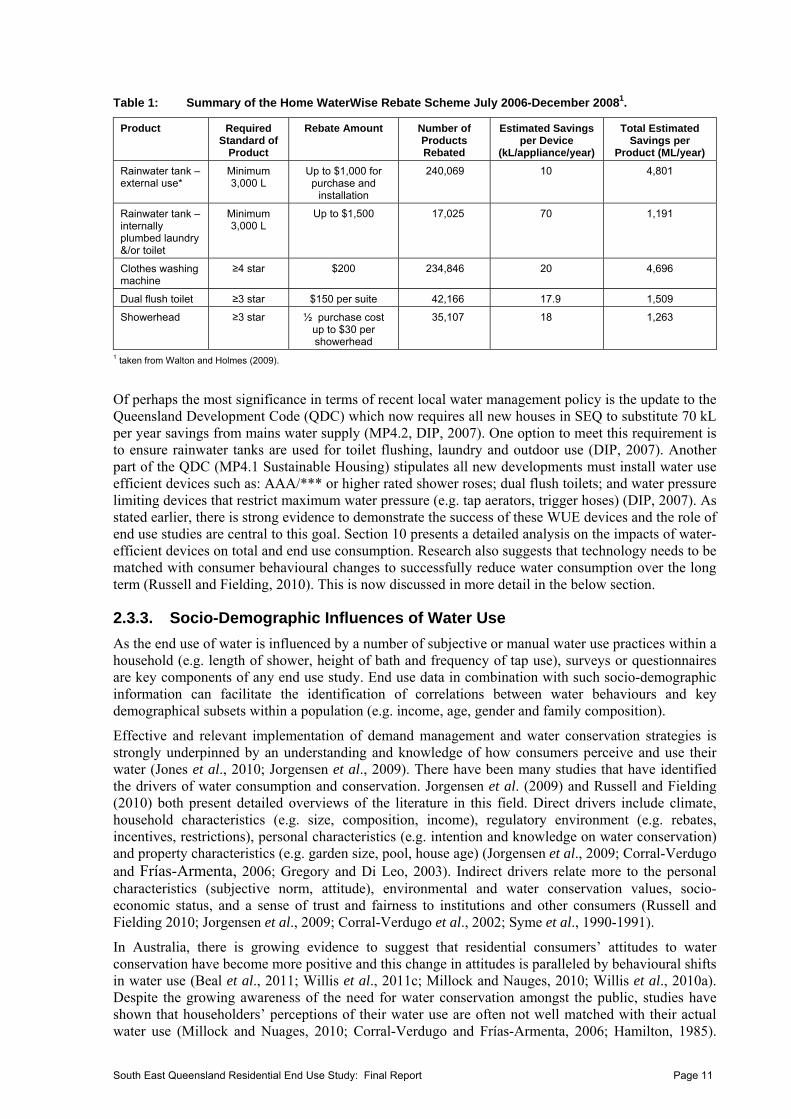
Table 1: Summary of the Home WaterWise Rebate Scheme July 2006-December 20081.
Product Required Standard of
Product
Rebate Amount Number of Products Rebated
Estimated Savings per Device
(kL/appliance/year)
Total Estimated Savings per
Product (ML/year)
Rainwater tank – external use*
Minimum 3,000 L
Up to $1,000 for purchase and
installation
240,069 10 4,801
Rainwater tank – internally plumbed laundry &/or toilet
Minimum 3,000 L
Up to $1,500 17,025 70 1,191
Clothes washing machine
≥4 star $200 234,846 20 4,696
Dual flush toilet ≥3 star $150 per suite 42,166 17.9 1,509
Showerhead ≥3 star ½ purchase cost up to $30 per showerhead
35,107 18 1,263
1 taken from Walton and Holmes (2009).
Of perhaps the most significance in terms of recent local water management policy is the update to the Queensland Development Code (QDC) which now requires all new houses in SEQ to substitute 70 kL per year savings from mains water supply (MP4.2, DIP, 2007). One option to meet this requirement is to ensure rainwater tanks are used for toilet flushing, laundry and outdoor use (DIP, 2007). Another part of the QDC (MP4.1 Sustainable Housing) stipulates all new developments must install water use efficient devices such as: AAA/*** or higher rated shower roses; dual flush toilets; and water pressure limiting devices that restrict maximum water pressure (e.g. tap aerators, trigger hoses) (DIP, 2007). As stated earlier, there is strong evidence to demonstrate the success of these WUE devices and the role of end use studies are central to this goal. Section 10 presents a detailed analysis on the impacts of water-efficient devices on total and end use consumption. Research also suggests that technology needs to be matched with consumer behavioural changes to successfully reduce water consumption over the long term (Russell and Fielding, 2010). This is now discussed in more detail in the below section.
2.3.3. Socio-Demographic Influences of Water Use
As the end use of water is influenced by a number of subjective or manual water use practices within a household (e.g. length of shower, height of bath and frequency of tap use), surveys or questionnaires are key components of any end use study. End use data in combination with such socio-demographic information can facilitate the identification of correlations between water behaviours and key demographical subsets within a population (e.g. income, age, gender and family composition).
Effective and relevant implementation of demand management and water conservation strategies is strongly underpinned by an understanding and knowledge of how consumers perceive and use their water (Jones et al., 2010; Jorgensen et al., 2009). There have been many studies that have identified the drivers of water consumption and conservation. Jorgensen et al. (2009) and Russell and Fielding (2010) both present detailed overviews of the literature in this field. Direct drivers include climate, household characteristics (e.g. size, composition, income), regulatory environment (e.g. rebates, incentives, restrictions), personal characteristics (e.g. intention and knowledge on water conservation) and property characteristics (e.g. garden size, pool, house age) (Jorgensen et al., 2009; Corral-Verdugo and Frías-Armenta, 2006; Gregory and Di Leo, 2003). Indirect drivers relate more to the personal characteristics (subjective norm, attitude), environmental and water conservation values, socio-economic status, and a sense of trust and fairness to institutions and other consumers (Russell and Fielding 2010; Jorgensen et al., 2009; Corral-Verdugo et al., 2002; Syme et al., 1990-1991).
In Australia, there is growing evidence to suggest that residential consumers’ attitudes to water conservation have become more positive and this change in attitudes is paralleled by behavioural shifts in water use (Beal et al., 2011; Willis et al., 2011c; Millock and Nauges, 2010; Willis et al., 2010a). Despite the growing awareness of the need for water conservation amongst the public, studies have shown that householders’ perceptions of their water use are often not well matched with their actual water use (Millock and Nuages, 2010; Corral-Verdugo and Frías-Armenta, 2006; Hamilton, 1985).
South East Queensland Residential End Use Study: Final Report Page 11

The mismatch between water use perceptions and outcomes is one that echoes the low correspondence that is often found between attitudes and behaviour (Kraus, 1995; Dolnicar and Hurlimann, 2010). Kantola et al. (1984), for example, showed that peoples’ self-reported attitudes toward energy conservation and their actual energy consumption differed and observed that people reduce the dissonance between attitudes and behaviour by bolstering or reaffirming their initial attitude (Kantola et al., 1984). Others describe the differences between beliefs and actual behaviour as more of a conflict between good intentions and difficulties in actually acting on them (Anker-Nilssen, 2003). The key socio-demographical influences on water consumption are discussed in Section 13.
2.3.4. Water-Energy Nexus Overview
It is becoming increasingly accepted that the simultaneous management of water and energy efficiency is essential in addressing the future management of climate change adaptation strategies (Fidar et al., 2010; Solomon et al., 2007; Gleick et al., 2010). The conflict between water use and associated energy consumption is often referred to as the water-energy nexus. This is particularly relevant in an urban context as studies continue to demonstrate the significant role that the urban resident plays in consuming water and energy resources (Kenway et al., 2011; Lenzen and Peters, 2010; Kenway et al., 2008; Cheng, 2002; Koomey et al., 1995). Managing such interconnected resources has significant implications on the savings (or production) of greenhouse gas emissions (Kenway et al., 2011; Golden et al., 2010; Clarke et al., 2009). As Fidar et al. (2010) and Maas (2009) observe, managing water demand through water efficient technology and behavioural changes has strong implications for reducing greenhouse gas emissions as well as conserving potable water supplies. This argument becomes stronger when one considers the acceleration of economic development and the subsequent rise in living standards in some developing countries (Pakula and Stamminger, 2010; Pachauri, 2004). Thus, it should be recognised that the link between water and energy use is inescapable and needs to be considered in managing future sustainable development.
The association between water end use residential appliances and fixtures and energy is briefly explored later in this report (Section 14).
2.4. Residential Water End Use Monitoring Approaches
2.4.1. Introduction
Water consumption does not always follow a normal distribution, as the high water users can strongly skew results. Similarly, water consumption patterns and behaviours are highly varied amongst households based on socio-demographics, house size, climate, family composition, water appliances, cultural practices and climate, to name just a few factors. As the end use of water is influenced by a number of subjective factors within a household, surveys or questionnaires are a key component of any end use study, regardless of technology used. Where resources are limited, often household surveys on water use behaviours are the only basis for reporting end uses (e.g. Sivakumaran and Aramaki, 2010). The following sections describe the two tiers of end use measurements based on the sophistication of the metering and data capture technology.
2.4.2. Typical End Use Approaches
Most end use studies have a mixed method approach that uses some level of technology with the data capture together with household surveys and/or existing statistical information sourced from various documents (e.g. census data, council billing data, previous reports). In some instances, residential water demand and end use volumes are predicted using a variety of data. For example, Blokker et al. (2010) simulated residential demand with a stochastic end use model. In this study, the water end use types were compiled from data; frequency of water fixture/appliance use was retrieved from previous household water surveys and intensity of use was determined from water use surveys and technical information from the stock appliance manufacturers. However, this approach can lead to inaccuracies, particularly for subjective end uses such as showers and taps. Additionally, reported appliance flow rates from manufacturers are not always the same as actual measured flow rates, as was found by Mead and Aravinthan (2009). Therefore, disaggregating end uses from actual long term measurement and analysis is considered the most robust and accurate approach.
South East Queensland Residential End Use Study: Final Report Page 12
South East Queensland Residential End Use Study: Final Report Page 13
2.4.3. Advanced End Use Measurement
Advanced end use measurement encompasses a range of attributes associated with all components of an end use study, and is not just limited to improved data capture. Advances in methods for data capture, transfer, storage and analysis have improved the resolution of water volume data and made transfer and collection of data substantially more time efficient. Giurco et al. (2008) considers ‘smart metering’ to have the following key elements: real time monitoring, high resolution interval metering (≥ 10 seconds), automated water meter reading (e.g. drive by, GPRS) and access to data from the internet.
Willis et al. (2009a) used a mixed method approach of high resolution water meters (0.014 L/pulse), 10 second interval data logging and detailed household stock inventories to measure and characterise the end uses of 151 dwellings on the Gold Coast. With this level of detail, sophisticated statistical analysis and water demand modelling can be performed with a much higher degree of certainty and fewer (often critical) assumptions embedded within the results. Indeed, Arbués et al. (2003) argue that water pricing modelling, particularly when incorporating time-of-use-tariffs, will only really be useful if a high level of detailed data input data is used.
Data transfer has also improved in recent times, enabling stored data from the loggers to be transferred remotely from the site. Such examples include drive-by technology where data is uploaded while driving past the metered property (e.g. Britton et al., 2009) or data is sent wirelessly via a GPRS system (i.e. email) from the loggers to an external office computer (e.g. Mead and Aravinthan, 2009).
Information on the social and behavioural aspects of metered properties, along with an audit of water appliance and fixtures, is absolutely essential for trace flow analysis (Athuraliya et al., 2008; White et al., 2004). Software such as Trace Wizard® has provided a key link between measured data and end use disaggregation (DeOreo and Mayer, 1999). However, without a stock inventory and information on water use behaviour/patterns for each dwelling it would be more difficult to create accurate end use templates. Ultimately, a diary should be kept for a week or more, recording the time and nature of as many water events as possible at the metered dwelling. Retrospective analysis could then identify the water event with the trace flow and match the end use type. Having the benefit of a water diary is not always possible and it requires a high level of commitment from the participants. Nevertheless, this was part of the advanced end use measurement approach for the SEQREUS study and has, to date, had an excellent return rate from the participants. Others such as O’Toole et al. (2009) and Wutich (2009) have also observed self-reported water usage via diaries can be more accurate than verbal estimations during interviews, especially for some end uses such as toilets (O’Toole et al., 2009).
2.5. Typical Residential End Uses A summary of recent end use studies outlining methods and selected results is presented in Table 2. In Australia, there have been only a few end use studies using a combination of metering technology, household surveys and end use software (i.e. Trace Wizard®) (Table 2). There are two frequently cited studies which have been conducted earlier; one in Perth (Loh and Coghlan, 2003) which has now been updated (Water Corporation, 2011) and the other in Melbourne (Roberts, 2005) which also has some updated publications (e.g. Gato-Trinidad et al., 2011). Willis et al. (2010a, 2010b, 2011a, 2011b) have reported more recently on water end uses from 151 dwellings in a development serviced by dual reticulated supplies (recycled water and mains water). Mead and Aravinthan (2009) reported on a small study of 10 residential properties in Toowoomba, west of Brisbane, Queensland. Internationally, several studies have been conducted in the United States of America (Mayer et al., 2004; DeOreo et al., 2001) as well as a recent study in New Zealand (Heinrich, 2008). Water end use studies are becoming more mainstream and many more are being planned internationally.
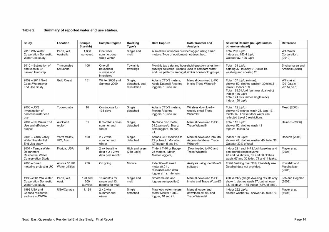
Table 2: Summary of reported water end use studies.
Study Location Sample Size (hh)
Sample Regime Dwelling Type/s
Data Capture Data Transfer and Analysis
Selected Results (in L/p/d unless otherwise stated)
Reference
2010 WA Water Corporation Domestic Water Use study
Perth, WA, Australia
1,868 surveyed
One week summer, one week winter
Single and multi
A small but unknown number logged using smart meters. Type of equipment not described.
Total 290 L/p/d Indoor av. 153.4 L/p/d Outdoor av. 126 L/p/d
WA Water Corporation. (2010)
2010 – Estimation of end uses in Sri Lankan township
Trincomalee Sri Lanka
106 One off household surveys and interviews
Township dwellings
Monthly tap data and household questionnaires from surveys collected. Results used to compare water end use patterns amongst similar household groups.
Total 139 L/p/d: bathing 37, laundry 21, toilet 19, washing and cooking 26
Sivakumaran and Aramaki (2010)
2009 – 2011 Gold Coast Watersaver End Use Study
Gold Coast 151 Winter 2008 and Summer 2009
Single, detached, dual reticulation
Actaris CT5-S meters, Aegis Datacell R series loggers, 10 sec. int.
Manual download to PC in-situ Trace Wizard®
Total 157 L/p/d (winter): shower 50, clothes washer, 30toilet 21, leaks 2.Indoor 139. Total 183.6 L/p/d (summer dual retic) Indoor 136 L/p/d Total 171.9 (summer single retic) Indoor 150 L/p/d
Willis et al. (2010a,b,c ; 2011a,bc,d)
2008 –USQ Investigation of domestic water end use
Toowoomba 10 Continuous for 138 days
Single detached
Actaris CT5-S meters, Monita R series loggers, 10 sec. int.
Wireless download – weekly email Trace Wizard®
Total 112 L/p/d: shower 49 clothes wash 25, taps 17, toilets 14. Low outdoor water use reflected Level 5 restrictions.
Mead (2008)
2007 – NZ Water End Use and efficiency project
Auckland region
51 6 months: across summer and winter
Single, detached
Neptune disc meter, 34.2 pulses/L, Branz data loggers, 10 sec int.
Manual download to PC. Trace Wizard®
Total 112 L/p/d: shower 50, clothes wash 43 taps 21, toilets 33
Heinrich (2006)
2005 – Yarra Valley Water Residential End Use study
Yarra Valley, VIC, Aust.
100 2 x 2 wks summer and winter
Single detached
Actaris CT5 modified to 72 pulses/L. Monatec XT logger, 5 sec int.
Manual download into MS Access database. Trace Wizard®
Indoor 169 L/p/d: shower 49, clothes washer 40, toilet 30. Outdoor 32% of total
Roberts (2005)
2004 - Tampa Water Department Residential Water Conservation Study
Florida, USA 26 2 wk baseline data + 2 x 2 wk data post retrofit
High end users (230 L/p/d)
Trident T-10 or Badger 25 meters, Meter-Master loggers,
Downloaded to PC and Trace Wizard®
Indoor 291 and 147 L/p/d (baseline and post retrofit respectively): 48 and 34 shower, 55 and 30 clothes wash, 67 and 30 toilet, 71 and14 leaks.
Mayer et al. (2004)
2003 – Smart metering project in UK
Across 10 UK Water utilities
250 On going Mixture Indentiflow® smart meter (0.01 L resolution) and data logger at 1s. intervals
Analysis using Identiflow® software
Toilet flushing over 30% total daily use. Detailed data not provided.
Kowalski and Marshallsay (2005)
1998–2001 WA Water Corporation Domestic Water Use study
Perth, WA, Aust.
120 and 600
surveys
18 months for single and 13 months for multi
Single and multi
Smart meters and loggers (unspecified)
Manual download to PC in-situ and Trace Wizard®
420 kL/hh/y (single dwelling results only shown): clothes wash 27, bath/shower 33, toilets 21. 155 indoor (42% of total).
Loh and Coghlan (2003)
1998 USA and Canada residential end use – AWWA
USA/Canada 1,188 2 x 2 wks summer and winter
Single detached
Magnetic water meters, Meter Master 100EL logger, 10 sec int.
Manual logger and download ex-situ and Trace Wizard®
Indoor 262 L/p/d: clothes washer 57, shower 44, toilet 70.
Mayer et al. (1998)
South East Queensland Residential End Use Study: Final Report Page 14
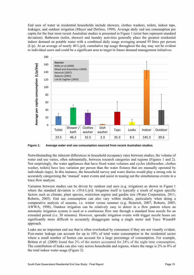
End uses of water in residential households include showers, clothes washers, toilets, indoor taps, leakages, and outdoor irrigation (Mayer and DeOreo, 1999). Average daily end use consumption per capita for the four most recent Australian studies is presented in Figure 1 (error bars represent standard deviation). Bathroom (toilet, shower) and laundry activities generally place the greatest residential indoor demand on potable water with a combined daily usage averaging around 95 litres per person (L/p). At an average of nearly 40 L/p/d, cumulative tap usage throughout the day may not be evident to individual users and could be a significant area to target in future demand management initiatives.
ToiletShower /bath
Clotheswasher
Dishwasher
Taps Leaks Indoor Outdoor
Series1 23.5 46.2 32.5 2.3 35.3 8.3 145.3 39.6
0
20
40
60
80
100
120
140
160
180
Average per capita consumption (L/p/day) Sources:
Willis et al (2009)Mead and Aravinthan (2009)Heinrich (2007)Roberts (2005)Loh & Coghlan (2003)
Figure 1: Average water end use consumption sourced from recent Australian studies.
Notwithstanding the inherent differences in household occupancy rates between studies, the volume of water end use varies, often substantially, between research categories and regions (Figures 1 and 2). Not surprisingly, the water appliances that have fixed water volumes and cycles (dishwasher, clothes washer, toilets) have less variation per person than the water fixtures that are manually operated by individuals (taps). In this instance, the household survey and water diaries would play a strong role in accurately categorising the ‘manual’ water events and assist in teasing out the simultaneous events in a trace flow analysis.
Variation between studies can be driven by outdoor end uses (e.g. irrigation) as shown in Figure 1 where the standard deviation is ±39.6 L/p/d. Irrigation itself is typically a result of region specific factors such as climate, plant species, restriction regime and garden size (Water Corporation, 2011; Roberts, 2005). End use consumption can also vary within studies, particularly when doing a comparative analysis of seasons, i.e. winter versus summer (e.g. Heinrich, 2007; Roberts, 2005; AWWA, 1998). Outdoor irrigation can be relatively easy to detect in a flow pattern where an automatic irrigation system is used or a continuous flow rate through a standard hose nozzle for an extended period (i.e. 30 minutes). However, sporadic irrigation events with trigger nozzle hoses are significantly more difficult to accurately disaggregate using a single meter and Trace Wizard® approach.
Leaks are an important end use that is often overlooked by consumers if they are not visually evident. Post-meter leakage can account for up to 10% of total water consumption in the residential sector where a small number of homes can account for a large percentage of consumption. For example, Britton et al. (2009) found that 2% of the meters accounted for 24% of the night time consumption. The contribution of leaks can also vary across households and regions, where the range is 2% to 8% of the total indoor water usage (Figure 2).
South East Queensland Residential End Use Study: Final Report Page 15
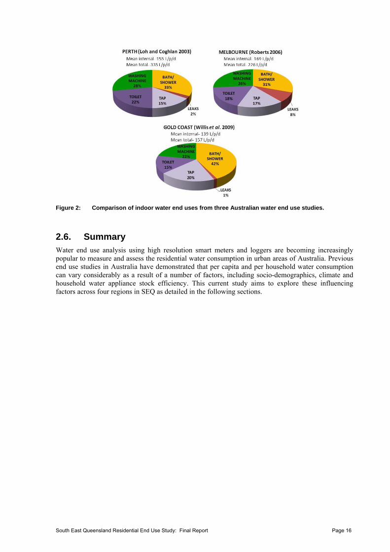
Figure 2: Comparison of indoor water end uses from three Australian water end use studies.
2.6. Summary Water end use analysis using high resolution smart meters and loggers are becoming increasingly popular to measure and assess the residential water consumption in urban areas of Australia. Previous end use studies in Australia have demonstrated that per capita and per household water consumption can vary considerably as a result of a number of factors, including socio-demographics, climate and household water appliance stock efficiency. This current study aims to explore these influencing factors across four regions in SEQ as detailed in the following sections.
South East Queensland Residential End Use Study: Final Report Page 16
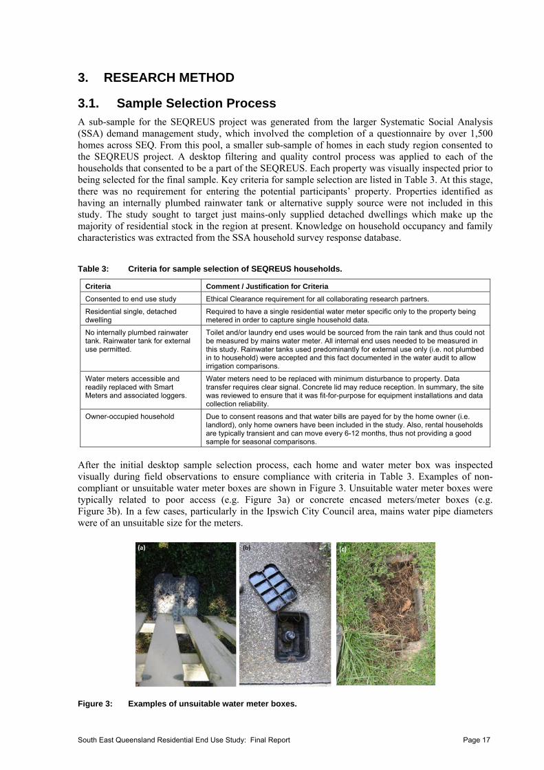
3. RESEARCH METHOD
3.1. Sample Selection Process A sub-sample for the SEQREUS project was generated from the larger Systematic Social Analysis (SSA) demand management study, which involved the completion of a questionnaire by over 1,500 homes across SEQ. From this pool, a smaller sub-sample of homes in each study region consented to the SEQREUS project. A desktop filtering and quality control process was applied to each of the households that consented to be a part of the SEQREUS. Each property was visually inspected prior to being selected for the final sample. Key criteria for sample selection are listed in Table 3. At this stage, there was no requirement for entering the potential participants’ property. Properties identified as having an internally plumbed rainwater tank or alternative supply source were not included in this study. The study sought to target just mains-only supplied detached dwellings which make up the majority of residential stock in the region at present. Knowledge on household occupancy and family characteristics was extracted from the SSA household survey response database.
Table 3: Criteria for sample selection of SEQREUS households.
Criteria Comment / Justification for Criteria
Consented to end use study Ethical Clearance requirement for all collaborating research partners.
Residential single, detached dwelling
Required to have a single residential water meter specific only to the property being metered in order to capture single household data.
No internally plumbed rainwater tank. Rainwater tank for external use permitted.
Toilet and/or laundry end uses would be sourced from the rain tank and thus could not be measured by mains water meter. All internal end uses needed to be measured in this study. Rainwater tanks used predominantly for external use only (i.e. not plumbed in to household) were accepted and this fact documented in the water audit to allow irrigation comparisons.
Water meters accessible and readily replaced with Smart Meters and associated loggers.
Water meters need to be replaced with minimum disturbance to property. Data transfer requires clear signal. Concrete lid may reduce reception. In summary, the site was reviewed to ensure that it was fit-for-purpose for equipment installations and data collection reliability.
Owner-occupied household Due to consent reasons and that water bills are payed for by the home owner (i.e. landlord), only home owners have been included in the study. Also, rental households are typically transient and can move every 6-12 months, thus not providing a good sample for seasonal comparisons.
After the initial desktop sample selection process, each home and water meter box was inspected visually during field observations to ensure compliance with criteria in Table 3. Examples of non-compliant or unsuitable water meter boxes are shown in Figure 3. Unsuitable water meter boxes were typically related to poor access (e.g. Figure 3a) or concrete encased meters/meter boxes (e.g. Figure 3b). In a few cases, particularly in the Ipswich City Council area, mains water pipe diameters were of an unsuitable size for the meters.
(c)
Figure 3: Examples of unsuitable water meter boxes.
South East Queensland Residential End Use Study: Final Report Page 17
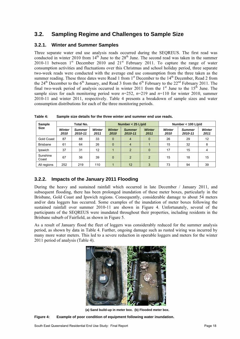
3.2. Sampling Regime and Challenges to Sample Size
3.2.1. Winter and Summer Samples
Three separate water end use analysis reads occurred during the SEQREUS. The first read was conducted in winter 2010 from 14th June to the 28th June. The second read was taken in the summer 2010-11 between 1st December 2010 and 21st February 2011. To capture the range of water consumption activities and fluctuations over this Christmas and school holiday period, three separate two-week reads were conducted with the average end use consumption from the three taken as the summer reading. These three dates were Read 1 from 1st December to the 14th December, Read 2 from the 24th December to the 6th January, and Read 3 from the 6th February to the 22nd February 2011. The final two-week period of analysis occurred in winter 2011 from the 1st June to the 15th June. The sample sizes for each monitoring period were n=252, n=219 and n=110 for winter 2010, summer 2010-11 and winter 2011, respectively. Table 4 presents a breakdown of sample sizes and water consumption distributions for each of the three monitoring periods.
Table 4: Sample size details for the three winter and summer end use reads.
Total No. Number < 25 L/p/d Number < 100 L/p/d Sample Size
Winter 2010
Summer 2010-11
Winter 2011
Winter 2010
Summer 2010-11
Winter 2011
Winter 2010
Summer 2010-11
Winter 2011
Gold Coast 87 68 33 0 4 0 26 29 12
Brisbane 61 64 26 0 4 1 15 32 8
Ipswich 37 31 12 1 2 0 17 15 4
Sunshine Coast
67 56 39 0 2 2 15 18 15
All regions 252 219 110 1 12 3 73 94 39
3.2.2. Impacts of the January 2011 Flooding
During the heavy and sustained rainfall which occurred in late December / January 2011, and subsequent flooding, there has been prolonged inundation of these meter boxes, particularly in the Brisbane, Gold Coast and Ipswich regions. Consequently, considerable damage to about 54 meters and/or data loggers has occurred. Some examples of the inundation of meter boxes following the sustained rainfall over summer 2010-11 are shown in Figure 4. Unfortunately, several of the participants of the SEQREUS were inundated throughout their properties, including residents in the Brisbane suburb of Fairfield, as shown in Figure 5.
As a result of January flood the fleet of loggers was considerably reduced for the summer analysis period, as shown by data in Table 4. Further, ongoing damage such as rusted wiring was incurred by many more water meters. This led to a severe reduction in operable loggers and meters for the winter 2011 period of analysis (Table 4).
(a) Sand build-up in meter box. (b) Flooded meter box.
Figure 4: Example of poor condition of equipment following water inundation.
South East Queensland Residential End Use Study: Final Report Page 18
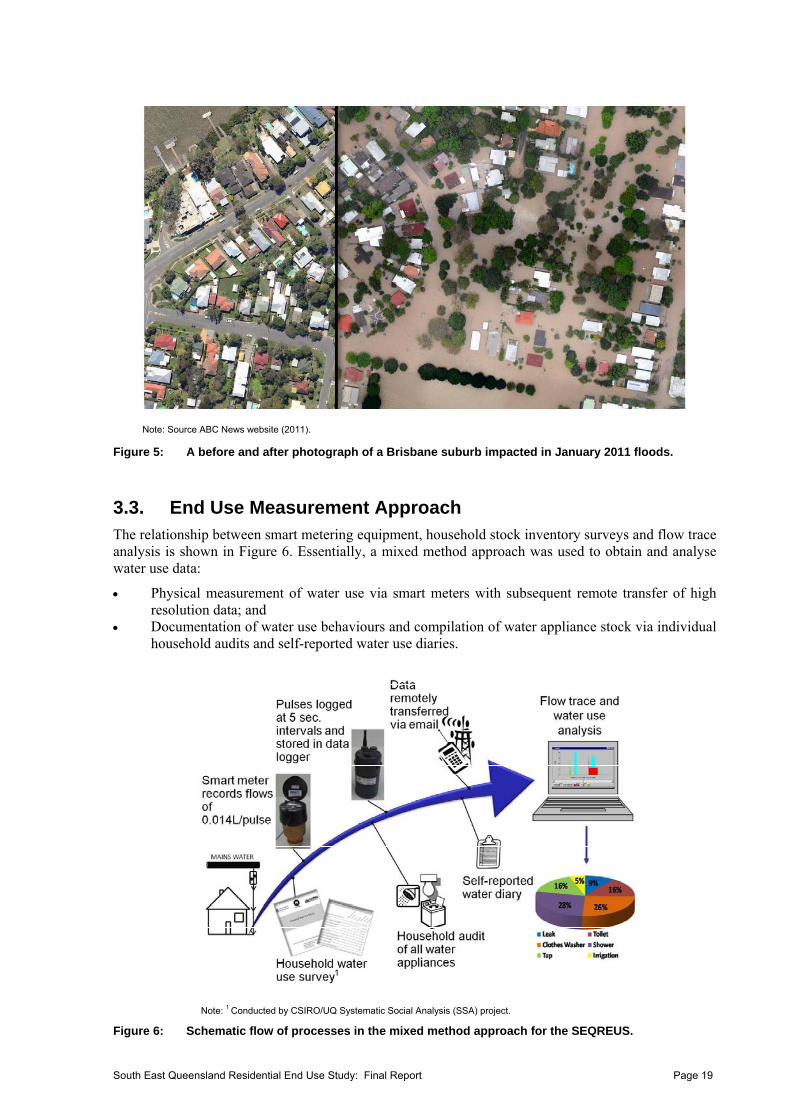
Note: Source ABC News website (2011).
Figure 5: A before and after photograph of a Brisbane suburb impacted in January 2011 floods.
3.3. End Use Measurement Approach The relationship between smart metering equipment, household stock inventory surveys and flow trace analysis is shown in Figure 6. Essentially, a mixed method approach was used to obtain and analyse water use data:
Physical measurement of water use via smart meters with subsequent remote transfer of high resolution data; and
Documentation of water use behaviours and compilation of water appliance stock via individual household audits and self-reported water use diaries.
1
Note: 1 Conducted by CSIRO/UQ Systematic Social Analysis (SSA) project.
Figure 6: Schematic flow of processes in the mixed method approach for the SEQREUS.
South East Queensland Residential End Use Study: Final Report Page 19
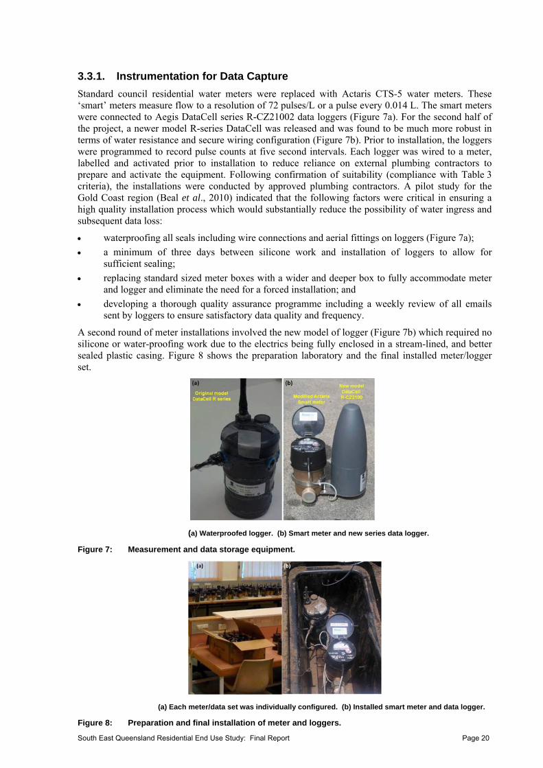
3.3.1. Instrumentation for Data Capture
Standard council residential water meters were replaced with Actaris CTS-5 water meters. These ‘smart’ meters measure flow to a resolution of 72 pulses/L or a pulse every 0.014 L. The smart meters were connected to Aegis DataCell series R-CZ21002 data loggers (Figure 7a). For the second half of the project, a newer model R-series DataCell was released and was found to be much more robust in terms of water resistance and secure wiring configuration (Figure 7b). Prior to installation, the loggers were programmed to record pulse counts at five second intervals. Each logger was wired to a meter, labelled and activated prior to installation to reduce reliance on external plumbing contractors to prepare and activate the equipment. Following confirmation of suitability (compliance with Table 3 criteria), the installations were conducted by approved plumbing contractors. A pilot study for the Gold Coast region (Beal et al., 2010) indicated that the following factors were critical in ensuring a high quality installation process which would substantially reduce the possibility of water ingress and subsequent data loss:
waterproofing all seals including wire connections and aerial fittings on loggers (Figure 7a);
a minimum of three days between silicone work and installation of loggers to allow for sufficient sealing;
replacing standard sized meter boxes with a wider and deeper box to fully accommodate meter and logger and eliminate the need for a forced installation; and
developing a thorough quality assurance programme including a weekly review of all emails sent by loggers to ensure satisfactory data quality and frequency.
A second round of meter installations involved the new model of logger (Figure 7b) which required no silicone or water-proofing work due to the electrics being fully enclosed in a stream-lined, and better sealed plastic casing. Figure 8 shows the preparation laboratory and the final installed meter/logger set.
(a) Waterproofed logger. (b) Smart meter and new series data logger.
Figure 7: Measurement and data storage equipment.
(a) Each meter/data set was individually configured. (b) Installed smart meter and data logger.
Figure 8: Preparation and final installation of meter and loggers.
South East Queensland Residential End Use Study: Final Report Page 20
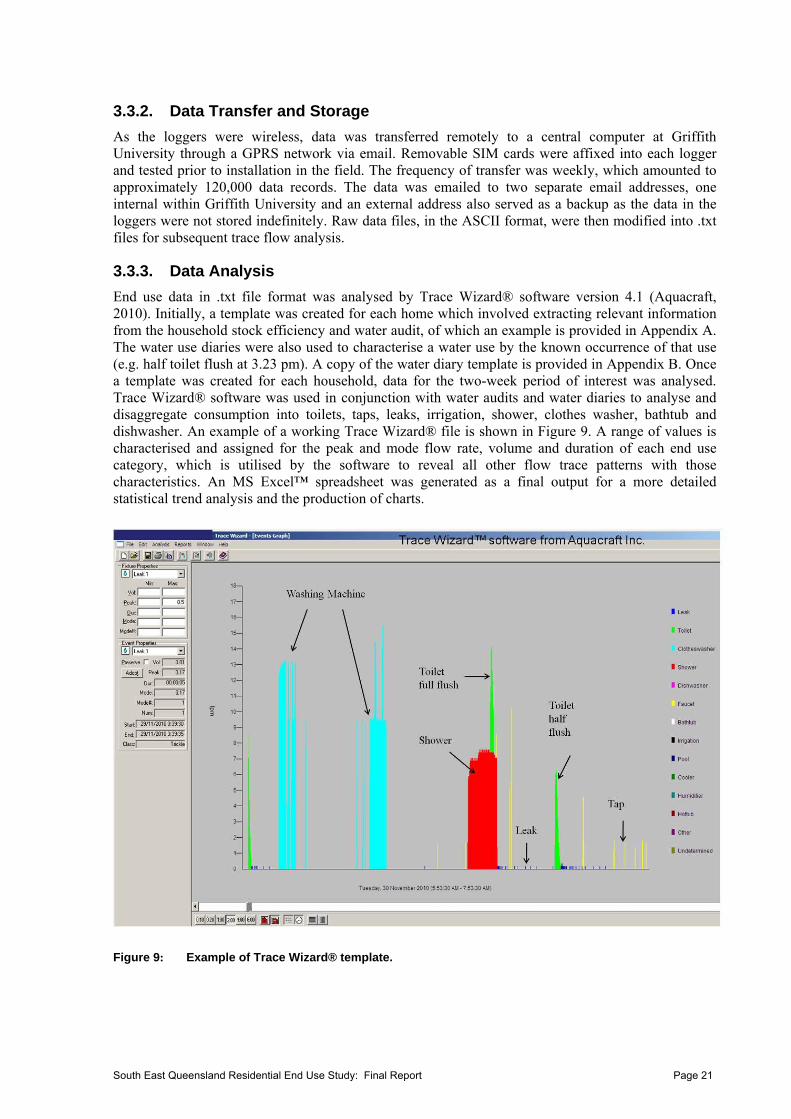
3.3.2. Data Transfer and Storage
As the loggers were wireless, data was transferred remotely to a central computer at Griffith University through a GPRS network via email. Removable SIM cards were affixed into each logger and tested prior to installation in the field. The frequency of transfer was weekly, which amounted to approximately 120,000 data records. The data was emailed to two separate email addresses, one internal within Griffith University and an external address also served as a backup as the data in the loggers were not stored indefinitely. Raw data files, in the ASCII format, were then modified into .txt files for subsequent trace flow analysis.
3.3.3. Data Analysis
End use data in .txt file format was analysed by Trace Wizard® software version 4.1 (Aquacraft, 2010). Initially, a template was created for each home which involved extracting relevant information from the household stock efficiency and water audit, of which an example is provided in Appendix A. The water use diaries were also used to characterise a water use by the known occurrence of that use (e.g. half toilet flush at 3.23 pm). A copy of the water diary template is provided in Appendix B. Once a template was created for each household, data for the two-week period of interest was analysed. Trace Wizard® software was used in conjunction with water audits and water diaries to analyse and disaggregate consumption into toilets, taps, leaks, irrigation, shower, clothes washer, bathtub and dishwasher. An example of a working Trace Wizard® file is shown in Figure 9. A range of values is characterised and assigned for the peak and mode flow rate, volume and duration of each end use category, which is utilised by the software to reveal all other flow trace patterns with those characteristics. An MS Excel™ spreadsheet was generated as a final output for a more detailed statistical trend analysis and the production of charts.
Figure 9: Example of Trace Wizard® template.
South East Queensland Residential End Use Study: Final Report Page 21
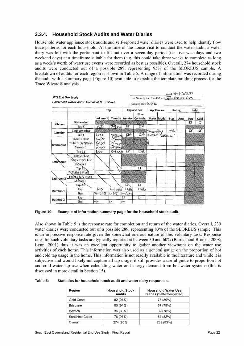
3.3.4. Household Stock Audits and Water Diaries
Household water appliance stock audits and self-reported water diaries were used to help identify flow trace patterns for each household. At the time of the house visit to conduct the water audit, a water diary was left with the participant to fill out over a seven-day period (i.e. five weekdays and two weekend days) at a timeframe suitable for them (e.g. this could take three weeks to complete as long as a week’s worth of water use events were recorded as best as possible). Overall, 274 household stock audits were conducted out of a possible 289, representing 95% of the SEQREUS sample. A breakdown of audits for each region is shown in Table 5. A range of information was recorded during the audit with a summary page (Figure 10) available to expedite the template building process for the Trace Wizard® analysis.
Figure 10: Example of information summary page for the household stock audit.
Also shown in Table 5 is the response rate for completion and return of the water diaries. Overall, 239 water diaries were conducted out of a possible 289, representing 83% of the SEQREUS sample. This is an impressive response rate given the somewhat onerous nature of this voluntary task. Response rates for such voluntary tasks are typically reported at between 30 and 60% (Baruch and Brooks, 2008; Lynn, 2001) thus it was an excellent opportunity to gather another viewpoint on the water use activities of each home. This information was also used as a general gauge on the proportion of hot and cold tap usage in the home. This information is not readily available in the literature and while it is subjective and would likely not capture all tap usage, it still provides a useful guide to proportion hot and cold water tap use when calculating water and energy demand from hot water systems (this is discussed in more detail in Section 15).
Table 5: Statistics for household stock audit and water dairy responses.
Region Household Stock Audits
Household Water Use Diaries (Self-Completed)
Gold Coast 82 (97%) 76 (89%)
Brisbane 80 (94%) 67 (79%)
Ipswich 36 (88%) 32 (78%)
Sunshine Coast 76 (97%) 64 (82%)
Overall 274 (95%) 239 (83%)
South East Queensland Residential End Use Study: Final Report Page 22
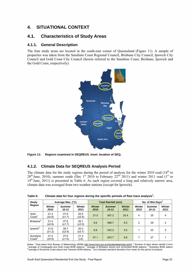
4. SITUATIONAL CONTEXT
4.1. Characteristics of Study Areas
4.1.1. General Description
The four study areas are located in the south-east corner of Queensland (Figure 11). A sample of properties was taken from the Sunshine Coast Regional Council, Brisbane City Council, Ipswich City Council and Gold Coast City Council (herein referred to the Sunshine Coast, Brisbane, Ipswich and the Gold Coast, respectively).
Figure 11: Regions examined in SEQREUS. Inset: location of SEQ.
4.1.2. Climate Data for SEQREUS Analysis Period
The climate data for the study regions during the period of analysis for the winter 2010 read (14th to 28th June, 2010), summer reads (Dec 1st 2010 to February 22nd 2011) and winter 2011 read (1st to 14th June, 2011) is presented in Table 6. As each region covered a long and relatively narrow area, climate data was averaged from two weather stations (except for Ipswich).
Table 6: Climate data for four regions during the specific periods of flow trace analysis1.
Average Max. (°C) Total Rainfall (mm) No. of Wet Days2 Study Region
Winter 2010
Summer 10-11
Winter 2011
Winter 2010
Summer 10-11
Winter 2011
Winter 2010
Summer 10-11
Winter 2011
Gold Coast3
21.3 (±0.8)
27.9 (±1.7)
20.5 (±2.9)
21.5 567.2 20.4 4 25 4
Brisbane4 21.4 (±0.9)
27.9 (±1.7)
20.1 (±3.5)
9.6 488.7 6.5 2 29 2
Ipswich5 21.8 (±1.2)
28.7 (±2.9)
20.3 (±3.7)
8.8 342.2 9.2 1 22 2
Sunshine Coast6
21.4 (±0.9)
27.6 (±1.6)
21.3 (±3)
47.1 543.7 8.6 7 27 1
Notes: 1 Data taken from Bureau of Meteorology (BOM) http://www.bom.gov.au/climate/data/index.shtml; 2 Number of days where rainfall ≥1mm; 3 average of Coolangatta and Gold Coast BOM stations; 4 average of Brisbane Airport and Archerfield BOM stations; 5 Amberley BOM station; 6 average of Sunshine Coast airport and Tewantin BOM stations, 7 (±x) indicates standard deviation from mean for the period of analysis.
South East Queensland Residential End Use Study: Final Report Page 23
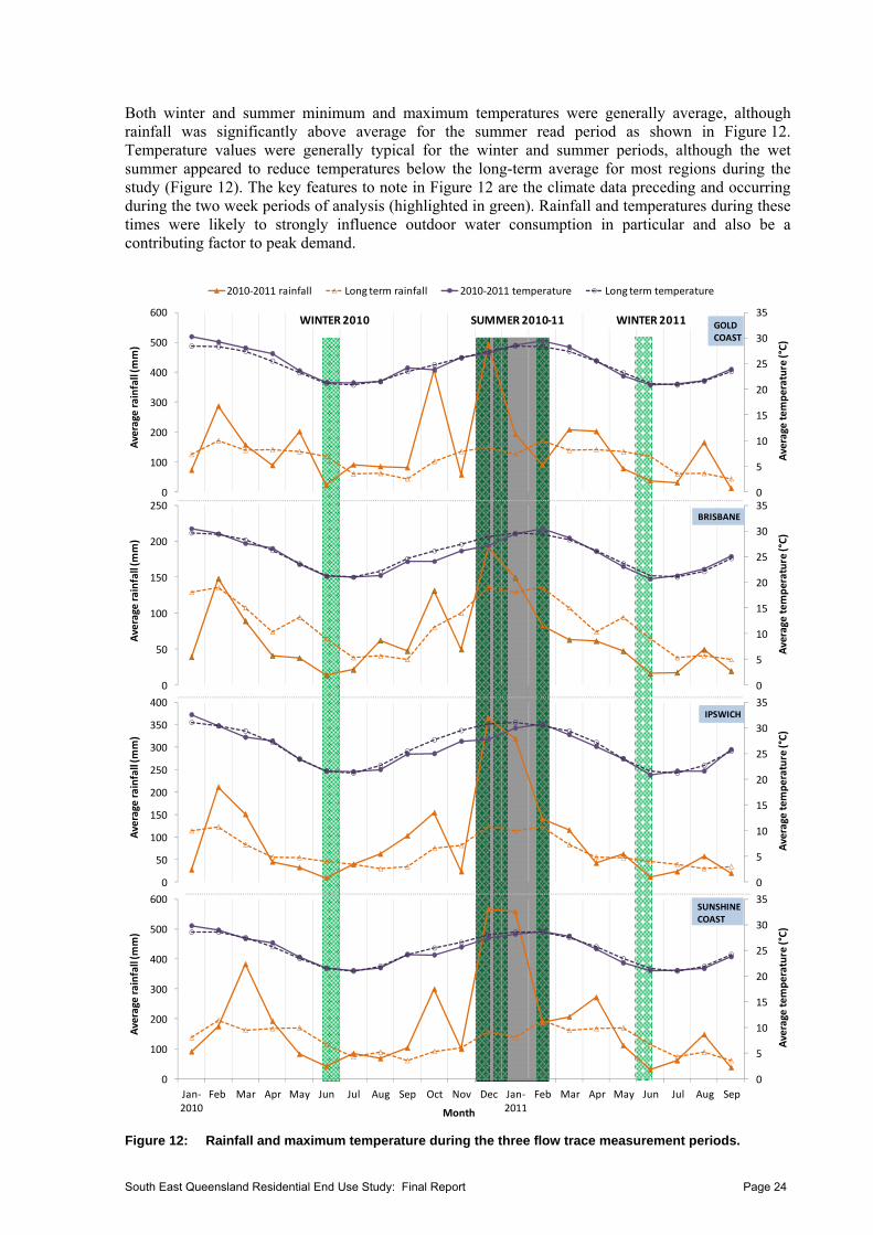
Both winter and summer minimum and maximum temperatures were generally average, although rainfall was significantly above average for the summer read period as shown in Figure 12. Temperature values were generally typical for the winter and summer periods, although the wet summer appeared to reduce temperatures below the long-term average for most regions during the study (Figure 12). The key features to note in Figure 12 are the climate data preceding and occurring during the two week periods of analysis (highlighted in green). Rainfall and temperatures during these times were likely to strongly influence outdoor water consumption in particular and also be a contributing factor to peak demand.
0
5
10
15
20
25
30
35
0
100
200
300
400
500
600
Average temperature (°C)
Average rainfall (m
m)
2010‐2011 rainfall Long term rainfall 2010‐2011 temperature Long term temperature
GOLDCOAST
0
5
10
15
20
25
30
35
0
50
100
150
200
250
Average temperature (°C)
Average rainfall (m
m)
BRISBANE
0
5
10
15
20
25
30
35
0
50
100
150
200
250
300
350
400
Average temperature (°C)
Average rainfall (m
m)
IPSWICH
0
5
10
15
20
25
30
35
0
100
200
300
400
500
600
Jan‐2010
Feb Mar Apr May Jun Jul Aug Sep Oct Nov Dec Jan‐2011
Feb Mar Apr May Jun Jul Aug Sep
Average temperature (°C)
Average rainfall (m
m)
Month
SUNSHINE COAST
WINTER 2010 SUMMER 2010‐11 WINTER 2011
Figure 12: Rainfall and maximum temperature during the three flow trace measurement periods.
South East Queensland Residential End Use Study: Final Report Page 24
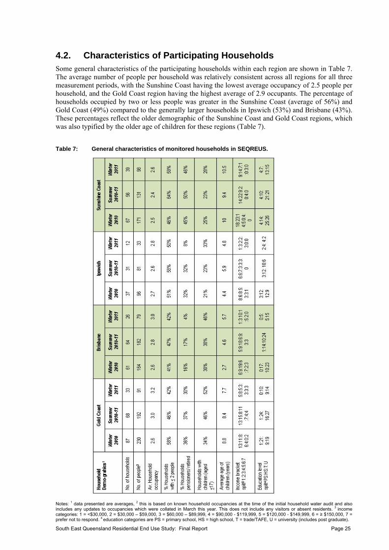
4.2. Characteristics of Participating Households Some general characteristics of the participating households within each region are shown in Table 7. The average number of people per household was relatively consistent across all regions for all three measurement periods, with the Sunshine Coast having the lowest average occupancy of 2.5 people per household, and the Gold Coast region having the highest average of 2.9 occupants. The percentage of households occupied by two or less people was greater in the Sunshine Coast (average of 56%) and Gold Coast (49%) compared to the generally larger households in Ipswich (53%) and Brisbane (43%). These percentages reflect the older demographic of the Sunshine Coast and Gold Coast regions, which was also typified by the older age of children for these regions (Table 7).
Table 7: General characteristics of monitored households in SEQREUS.
Notes: 1 data presented are averages, 2 this is based on known household occupancies at the time of the initial household water audit and also includes any updates to occupancies which were collated in March this year. This does not include any visitors or absent residents. 3 income categories: 1 = <$30,000, 2 = $30,000 – $59,000, 3 = $60,000 – $89,999, 4 = $90,000 - $119,999, 5 = $120,000 - $149,999, 6 = ≥ $150,000, 7 = prefer not to respond. 4 education categories are PS = primary school, HS = high school, T = trade/TAFE, U = university (includes post graduate).
South East Queensland Residential End Use Study: Final Report Page 25
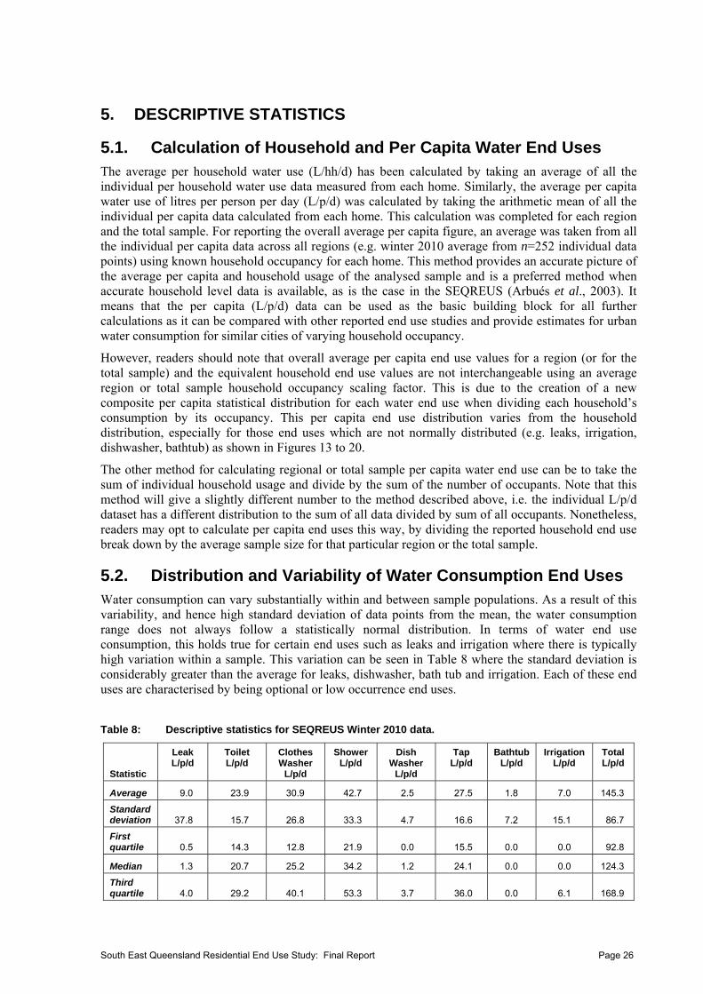
5. DESCRIPTIVE STATISTICS
5.1. Calculation of Household and Per Capita Water End Uses The average per household water use (L/hh/d) has been calculated by taking an average of all the individual per household water use data measured from each home. Similarly, the average per capita water use of litres per person per day (L/p/d) was calculated by taking the arithmetic mean of all the individual per capita data calculated from each home. This calculation was completed for each region and the total sample. For reporting the overall average per capita figure, an average was taken from all the individual per capita data across all regions (e.g. winter 2010 average from n=252 individual data points) using known household occupancy for each home. This method provides an accurate picture of the average per capita and household usage of the analysed sample and is a preferred method when accurate household level data is available, as is the case in the SEQREUS (Arbués et al., 2003). It means that the per capita (L/p/d) data can be used as the basic building block for all further calculations as it can be compared with other reported end use studies and provide estimates for urban water consumption for similar cities of varying household occupancy.
However, readers should note that overall average per capita end use values for a region (or for the total sample) and the equivalent household end use values are not interchangeable using an average region or total sample household occupancy scaling factor. This is due to the creation of a new composite per capita statistical distribution for each water end use when dividing each household’s consumption by its occupancy. This per capita end use distribution varies from the household distribution, especially for those end uses which are not normally distributed (e.g. leaks, irrigation, dishwasher, bathtub) as shown in Figures 13 to 20.
The other method for calculating regional or total sample per capita water end use can be to take the sum of individual household usage and divide by the sum of the number of occupants. Note that this method will give a slightly different number to the method described above, i.e. the individual L/p/d dataset has a different distribution to the sum of all data divided by sum of all occupants. Nonetheless, readers may opt to calculate per capita end uses this way, by dividing the reported household end use break down by the average sample size for that particular region or the total sample.
5.2. Distribution and Variability of Water Consumption End Uses Water consumption can vary substantially within and between sample populations. As a result of this variability, and hence high standard deviation of data points from the mean, the water consumption range does not always follow a statistically normal distribution. In terms of water end use consumption, this holds true for certain end uses such as leaks and irrigation where there is typically high variation within a sample. This variation can be seen in Table 8 where the standard deviation is considerably greater than the average for leaks, dishwasher, bath tub and irrigation. Each of these end uses are characterised by being optional or low occurrence end uses.
Table 8: Descriptive statistics for SEQREUS Winter 2010 data.
Statistic
Leak L/p/d
Toilet L/p/d
Clothes Washer
L/p/d
ShowerL/p/d
Dish Washer
L/p/d
Tap L/p/d
Bathtub L/p/d
IrrigationL/p/d
TotalL/p/d
Average 9.0 23.9 30.9 42.7 2.5 27.5 1.8 7.0 145.3
Standard deviation 37.8 15.7 26.8 33.3 4.7 16.6 7.2 15.1 86.7
First quartile 0.5 14.3 12.8 21.9 0.0 15.5 0.0 0.0 92.8
Median 1.3 20.7 25.2 34.2 1.2 24.1 0.0 0.0 124.3
Third quartile 4.0 29.2 40.1 53.3 3.7 36.0 0.0 6.1 168.9
South East Queensland Residential End Use Study: Final Report Page 26
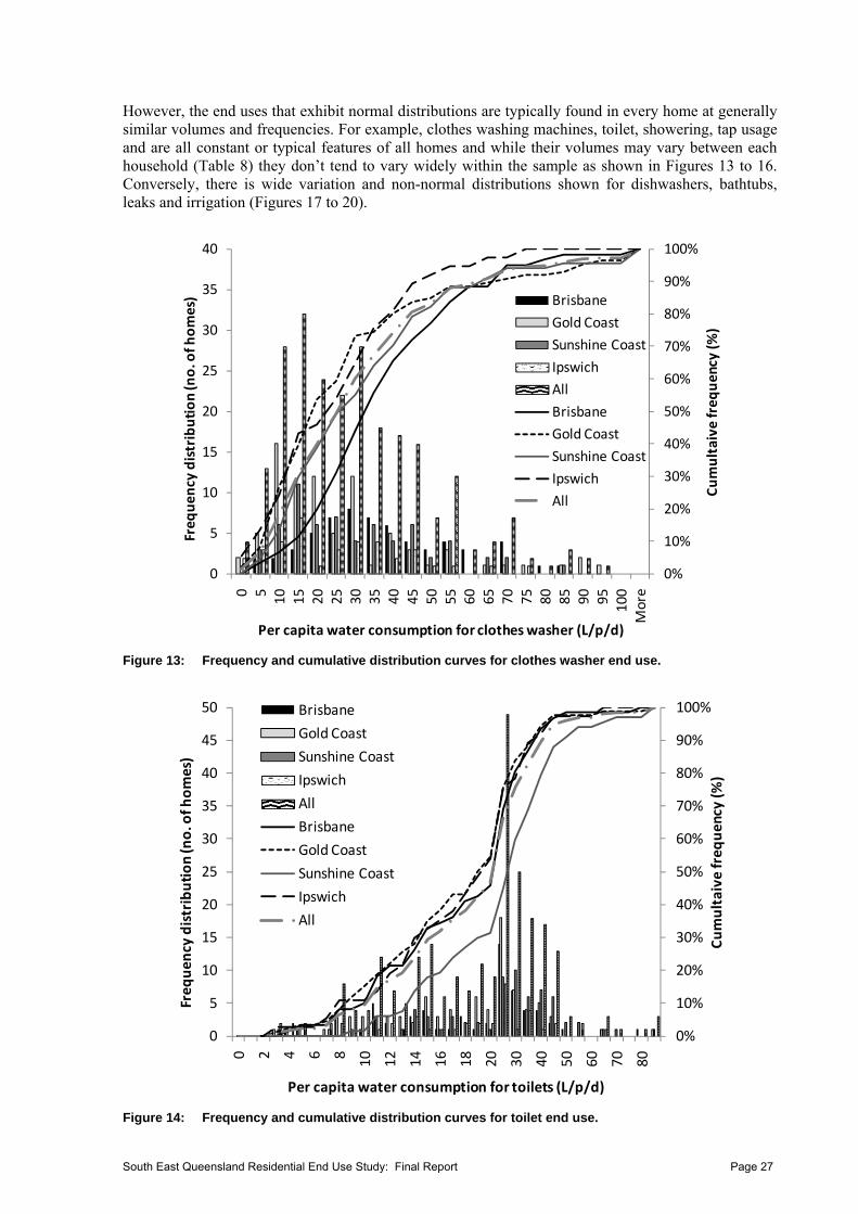
However, the end uses that exhibit normal distributions are typically found in every home at generally similar volumes and frequencies. For example, clothes washing machines, toilet, showering, tap usage and are all constant or typical features of all homes and while their volumes may vary between each household (Table 8) they don’t tend to vary widely within the sample as shown in Figures 13 to 16. Conversely, there is wide variation and non-normal distributions shown for dishwashers, bathtubs, leaks and irrigation (Figures 17 to 20).
0%
10%
20%
30%
40%
50%
60%
70%
80%
90%
100%
0
5
10
15
20
25
30
35
400 5101520253035404550556065707580859095
100
More
Cumultaive
frequency (%
)
Freq
uency distribution (n
o. of homes)
Per capita water consumption for clothes washer (L/p/d)
Brisbane
Gold Coast
Sunshine Coast
Ipswich
All
Brisbane
Gold Coast
Sunshine Coast
Ipswich
All
Figure 13: Frequency and cumulative distribution curves for clothes washer end use.
0%
10%
20%
30%
40%
50%
60%
70%
80%
90%
100%
0
5
10
15
20
25
30
35
40
45
50
0 2 4 6 8
10
12
14
16
18
20
30
40
50
60
70
80
Cumultaive freq
uency (%)
Frequency distribution (n
o. of h
omes)
Per capita water consumption for toilets (L/p/d)
Brisbane
Gold Coast
Sunshine Coast
Ipswich
All
Brisbane
Gold Coast
Sunshine Coast
Ipswich
All
Figure 14: Frequency and cumulative distribution curves for toilet end use.
South East Queensland Residential End Use Study: Final Report Page 27
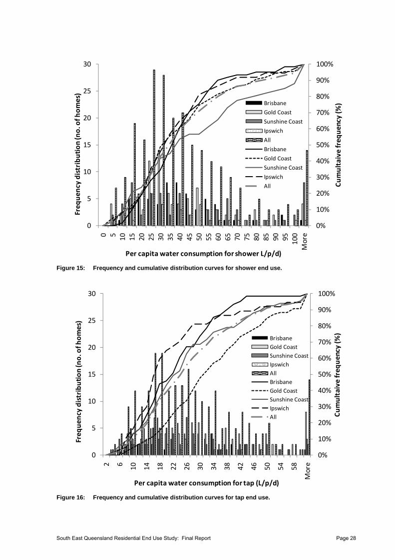
0%
10%
20%
30%
40%
50%
60%
70%
80%
90%
100%
0
5
10
15
20
25
30
0 510 15 20 25 30 35 40 45 50 55 60 65 70 75 80 85 90 95
100
More
Cumultaive freq
uency (%
)
Frequency distribution (no. of homes)
Per capita water consumption for shower L/p/d)
Brisbane
Gold Coast
Sunshine Coast
Ipswich
All
Brisbane
Gold Coast
Sunshine Coast
Ipswich
All
Figure 15: Frequency and cumulative distribution curves for shower end use.
0%
10%
20%
30%
40%
50%
60%
70%
80%
90%
100%
0
5
10
15
20
25
30
2 6
10
14
18
22
26
30
34
38
42
46
50
54
58
More
Cumultaive
freq
uency (%
)
Frequency distribution (n
o. of h
omes)
Per capita water consumption for tap (L/p/d)
Brisbane
Gold Coast
Sunshine Coast
Ipswich
All
Brisbane
Gold Coast
Sunshine Coast
Ipswich
All
Figure 16: Frequency and cumulative distribution curves for tap end use.
South East Queensland Residential End Use Study: Final Report Page 28
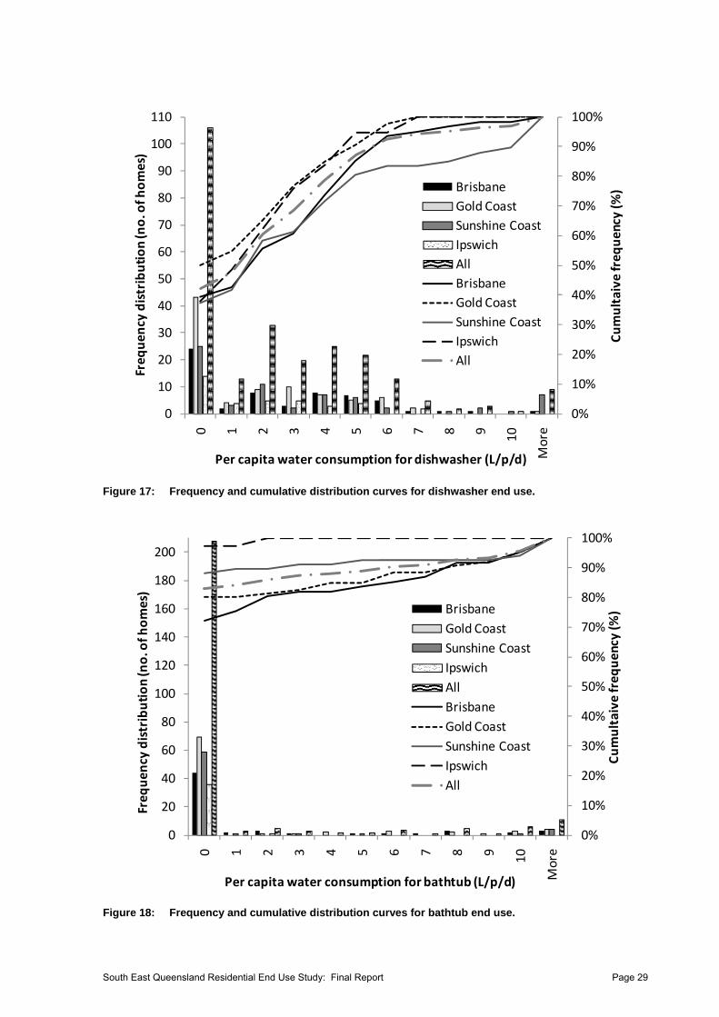
0%
10%
20%
30%
40%
50%
60%
70%
80%
90%
100%
0
10
20
30
40
50
60
70
80
90
100
110
0 1 2 3 4 5 6 7 8 9
10
More
Cumultaive frequency (%)
Frequency distribution (no. of homes)
Per capita water consumption for dishwasher (L/p/d)
Brisbane
Gold Coast
Sunshine Coast
Ipswich
All
Brisbane
Gold Coast
Sunshine Coast
Ipswich
All
Figure 17: Frequency and cumulative distribution curves for dishwasher end use.
0%
10%
20%
30%
40%
50%
60%
70%
80%
90%
100%
0
20
40
60
80
100
120
140
160
180
200
0 1 2 3 4 5 6 7 8 9
10
More
Cumultaive frequency (%
)
Frequency distribution (no. of homes)
Per capita water consumption for bathtub (L/p/d)
Brisbane
Gold Coast
Sunshine Coast
Ipswich
All
Brisbane
Gold Coast
Sunshine Coast
Ipswich
All
Figure 18: Frequency and cumulative distribution curves for bathtub end use.
South East Queensland Residential End Use Study: Final Report Page 29
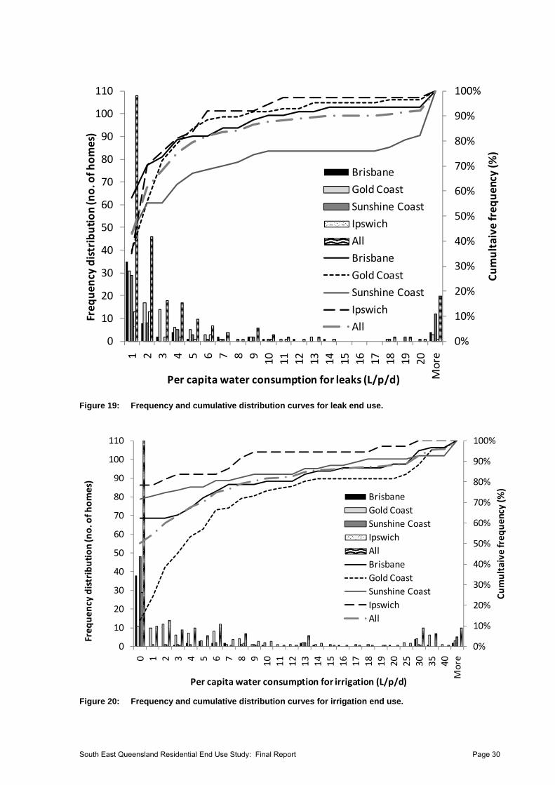
0%
10%
20%
30%
40%
50%
60%
70%
80%
90%
100%
0
10
20
30
40
50
60
70
80
90
100
110
1 2 3 4 5 6 7 8 9
10 11 12 13 14 15 16 17 18 19 20
More
Cumultaive
freq
uency (%)
Freq
uency distribution (no. of homes)
Per capita water consumption for leaks (L/p/d)
Brisbane
Gold Coast
Sunshine Coast
Ipswich
All
Brisbane
Gold Coast
Sunshine Coast
Ipswich
All
Figure 19: Frequency and cumulative distribution curves for leak end use.
0%
10%
20%
30%
40%
50%
60%
70%
80%
90%
100%
0
10
20
30
40
50
60
70
80
90
100
110
0 1 2 3 4 5 6 7 8 9101112131415161718192025303540
More
Cumultaive frequency (%)
Frequency distribution (no. of h
omes)
Per capita water consumption for irrigation (L/p/d)
Brisbane
Gold Coast
Sunshine Coast
Ipswich
All
Brisbane
Gold Coast
Sunshine Coast
Ipswich
All
Figure 20: Frequency and cumulative distribution curves for irrigation end use.
South East Queensland Residential End Use Study: Final Report Page 30

5.3. Winter 2010 End Use Event Statistics
5.3.1. Introduction
The following subsections present descriptive statistics on end use event frequencies, flow rates, mean volumes and durations. The data from winter 2010 has been used as it represents results from the largest sample size from the three reads throughout the SEQREUS. Therefore, it is considered the most robust in terms of representing the greatest variation in household characteristics, thus the strongest dataset in terms of statistical significance and cross regional variations. Additionally, the climate for the winter 2010 was reasonably representative of the long term averages (temperature and rainfall) for that sampling period. These justifications for primarily using the winter 2010 dataset is maintained throughout this document when reporting and discussing specific aspects of the SEQREUS results. Note that some parts of the tables are shaded grey. Due to the small sample size (dishwasher end use) or excessively high values (clothes washer end use), the numbers have been omitted.
5.3.2. End Use Event Frequencies
Tables 9, 10, 11 and 12 present end use event frequency statistics for winter 2010 for the Gold Coast, Brisbane, Ipswich and the Sunshine Coast, respectively.
Table 9: Gold Coast Winter End Use Event Frequency Statistics.
Frequency (events/day) Statistics
Half Flush Full Flush Tap Shower Bath Dishwasher Clothes Washer Irrigation
Mean 4.49 3.86 40.64 1.84 0.10 0.37 0.54 0.33
Std. 3.25 2.69 19.63 1.20 0.23 0.42 0.34 0.28
Skewness 0.83 1.25 0.77 1.55 2.48 1.28 0.30 0.94
Kurtosis 0.43 1.96 0.37 3.63 5.95 1.23 -0.84 0.43
1st Quartile 1.75 1.86 25.14 1.00 0.00 0.00 0.29 0.21
2nd Quartile 4.07 3.39 38.21 1.61 0.00 0.21 0.50 0.24
3rd Quartile 6.57 5.23 51.82 2.64 0.00 0.64 0.73 0.51
4th Quartile 14.07 12.93 93.29 6.37 1.00 1.57 1.21 1.14
Table 10: Brisbane Winter End Use Event Frequency Statistics.
Frequency (events/day) Statistics
Half Flush Full Flush Tap Shower Bath Dishwasher Clothes Washer Irrigation
Mean 4.87 4.21 58.70 2.13 0.13 0.55 0.71 0.12
Std. 3.97 2.68 33.42 1.99 0.28 0.68 0.56 0.19
Skewness 1.67 1.29 1.13 5.11 2.12 1.94 2.93 1.94
Kurtosis 3.99 1.67 1.90 33.79 3.36 5.15 14.28 3.68
1st Quartile 2.64 2.54 34.93 1.21 0.00 0.00 0.36 0.00
2nd Quartile 4.25 3.50 51.36 1.93 0.00 0.43 0.64 0.00
3rd Quartile 6.00 4.71 80.14 2.57 0.00 0.86 1.00 0.21
4th Quartile 21.21 13.36 175.14 15.46 1.14 3.21 3.79 0.79
South East Queensland Residential End Use Study: Final Report Page 31
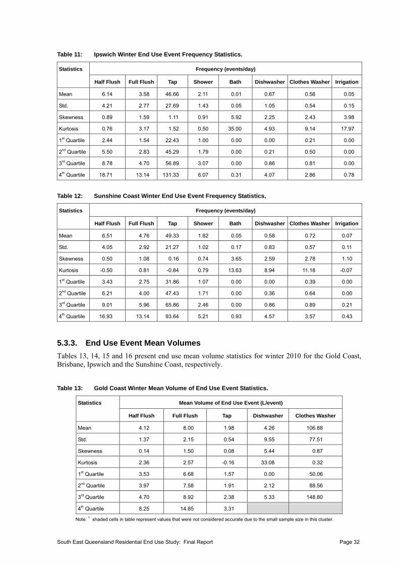
Table 11: Ipswich Winter End Use Event Frequency Statistics.
Frequency (events/day) Statistics
Half Flush Full Flush Tap Shower Bath Dishwasher Clothes Washer Irrigation
Mean 6.14 3.58 46.66 2.11 0.01 0.67 0.56 0.05
Std. 4.21 2.77 27.69 1.43 0.05 1.05 0.54 0.15
Skewness 0.89 1.59 1.11 0.91 5.92 2.25 2.43 3.98
Kurtosis 0.76 3.17 1.52 0.50 35.00 4.93 9.14 17.97
1st Quartile 2.44 1.54 22.43 1.00 0.00 0.00 0.21 0.00
2nd Quartile 5.50 2.83 45.29 1.79 0.00 0.21 0.50 0.00
3rd Quartile 8.78 4.70 56.89 3.07 0.00 0.86 0.81 0.00
4th Quartile 18.71 13.14 131.33 6.07 0.31 4.07 2.86 0.78
Table 12: Sunshine Coast Winter End Use Event Frequency Statistics.
Frequency (events/day) Statistics
Half Flush Full Flush Tap Shower Bath Dishwasher Clothes Washer Irrigation
Mean 6.51 4.76 49.33 1.82 0.05 0.58 0.72 0.07
Std. 4.05 2.92 21.27 1.02 0.17 0.83 0.57 0.11
Skewness 0.50 1.08 0.16 0.74 3.65 2.59 2.78 1.10
Kurtosis -0.50 0.81 -0.84 0.79 13.63 8.94 11.18 -0.07
1st Quartile 3.43 2.75 31.86 1.07 0.00 0.00 0.39 0.00
2nd Quartile 6.21 4.00 47.43 1.71 0.00 0.36 0.64 0.00
3rd Quartile 9.01 5.96 65.86 2.46 0.00 0.86 0.89 0.21
4th Quartile 16.93 13.14 93.64 5.21 0.93 4.57 3.57 0.43
5.3.3. End Use Event Mean Volumes
Tables 13, 14, 15 and 16 present end use mean volume statistics for winter 2010 for the Gold Coast, Brisbane, Ipswich and the Sunshine Coast, respectively.
Table 13: Gold Coast Winter Mean Volume of End Use Event Statistics.
Mean Volume of End Use Event (L/event) Statistics
Half Flush Full Flush Tap Dishwasher Clothes Washer
Mean 4.12 8.00 1.98 4.26 106.88
Std. 1.37 2.15 0.54 9.55 77.51
Skewness 0.14 1.50 0.08 5.44 0.87
Kurtosis 2.36 2.57 -0.16 33.08 0.32
1st Quartile 3.53 6.68 1.57 0.00 50.06
2nd Quartile 3.97 7.58 1.91 2.12 88.56
3rd Quartile 4.70 8.92 2.38 5.33 148.80
4th Quartile 8.25 14.85 3.31
Note: 1 shaded cells in table represent values that were not considered accurate due to the small sample size in this cluster.
South East Queensland Residential End Use Study: Final Report Page 32
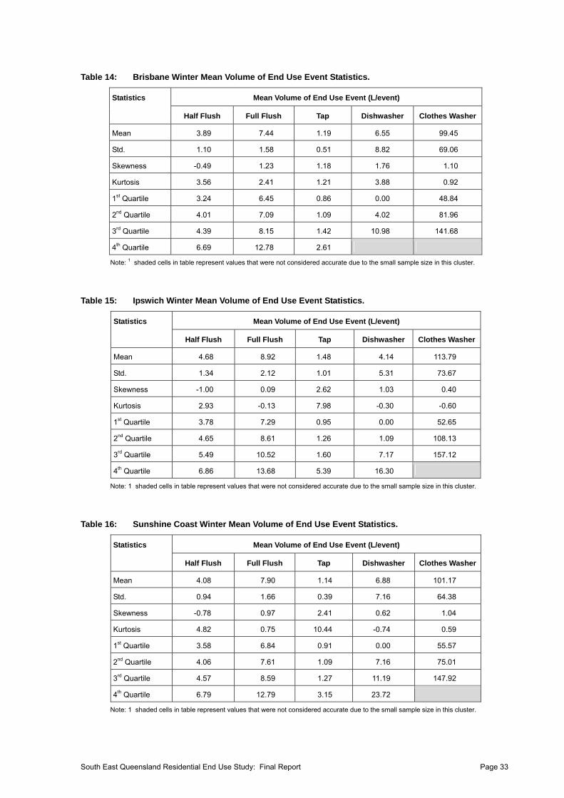
Table 14: Brisbane Winter Mean Volume of End Use Event Statistics.
Mean Volume of End Use Event (L/event) Statistics
Half Flush Full Flush Tap Dishwasher Clothes Washer
Mean 3.89 7.44 1.19 6.55 99.45
Std. 1.10 1.58 0.51 8.82 69.06
Skewness -0.49 1.23 1.18 1.76 1.10
Kurtosis 3.56 2.41 1.21 3.88 0.92
1st Quartile 3.24 6.45 0.86 0.00 48.84
2nd Quartile 4.01 7.09 1.09 4.02 81.96
3rd Quartile 4.39 8.15 1.42 10.98 141.68
4th Quartile 6.69 12.78 2.61
Note: 1 shaded cells in table represent values that were not considered accurate due to the small sample size in this cluster.
Table 15: Ipswich Winter Mean Volume of End Use Event Statistics.
Mean Volume of End Use Event (L/event) Statistics
Half Flush Full Flush Tap Dishwasher Clothes Washer
Mean 4.68 8.92 1.48 4.14 113.79
Std. 1.34 2.12 1.01 5.31 73.67
Skewness -1.00 0.09 2.62 1.03 0.40
Kurtosis 2.93 -0.13 7.98 -0.30 -0.60
1st Quartile 3.78 7.29 0.95 0.00 52.65
2nd Quartile 4.65 8.61 1.26 1.09 108.13
3rd Quartile 5.49 10.52 1.60 7.17 157.12
4th Quartile 6.86 13.68 5.39 16.30
Note: 1 shaded cells in table represent values that were not considered accurate due to the small sample size in this cluster.
Table 16: Sunshine Coast Winter Mean Volume of End Use Event Statistics.
Mean Volume of End Use Event (L/event) Statistics
Half Flush Full Flush Tap Dishwasher Clothes Washer
Mean 4.08 7.90 1.14 6.88 101.17
Std. 0.94 1.66 0.39 7.16 64.38
Skewness -0.78 0.97 2.41 0.62 1.04
Kurtosis 4.82 0.75 10.44 -0.74 0.59
1st Quartile 3.58 6.84 0.91 0.00 55.57
2nd Quartile 4.06 7.61 1.09 7.16 75.01
3rd Quartile 4.57 8.59 1.27 11.19 147.92
4th Quartile 6.79 12.79 3.15 23.72
Note: 1 shaded cells in table represent values that were not considered accurate due to the small sample size in this cluster.
South East Queensland Residential End Use Study: Final Report Page 33
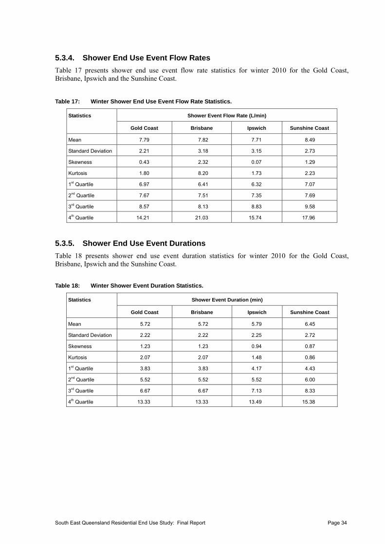
South East Queensland Residential End Use Study: Final Report Page 34
5.3.4. Shower End Use Event Flow Rates
Table 17 presents shower end use event flow rate statistics for winter 2010 for the Gold Coast, Brisbane, Ipswich and the Sunshine Coast.
Table 17: Winter Shower End Use Event Flow Rate Statistics.
Shower Event Flow Rate (L/min) Statistics
Gold Coast Brisbane Ipswich Sunshine Coast
Mean 7.79 7.82 7.71 8.49
Standard Deviation 2.21 3.18 3.15 2.73
Skewness 0.43 2.32 0.07 1.29
Kurtosis 1.80 8.20 1.73 2.23
1st Quartile 6.97 6.41 6.32 7.07
2nd Quartile 7.67 7.51 7.35 7.69
3rd Quartile 8.57 8.13 8.83 9.58
4th Quartile 14.21 21.03 15.74 17.96
5.3.5. Shower End Use Event Durations
Table 18 presents shower end use event duration statistics for winter 2010 for the Gold Coast, Brisbane, Ipswich and the Sunshine Coast.
Table 18: Winter Shower Event Duration Statistics.
Shower Event Duration (min) Statistics
Gold Coast Brisbane Ipswich Sunshine Coast
Mean 5.72 5.72 5.79 6.45
Standard Deviation 2.22 2.22 2.25 2.72
Skewness 1.23 1.23 0.94 0.87
Kurtosis 2.07 2.07 1.48 0.86
1st Quartile 3.83 3.83 4.17 4.43
2nd Quartile 5.52 5.52 5.52 6.00
3rd Quartile 6.67 6.67 7.13 8.33
4th Quartile 13.33 13.33 13.49 15.38
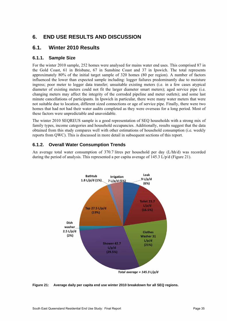
6. END USE RESULTS AND DISCUSSION
6.1. Winter 2010 Results
6.1.1. Sample Size
For the winter 2010 sample, 252 homes were analysed for mains water end uses. This comprised 87 in the Gold Coast, 61 in Brisbane, 67 in Sunshine Coast and 37 in Ipswich. The total represents approximately 80% of the initial target sample of 320 homes (80 per region). A number of factors influenced the lower than expected sample including: logger failures predominantly due to moisture ingress; poor meter to logger data transfer; unsuitable existing meters (i.e. in a few cases atypical diameter of existing meters could not fit the larger diameter smart meters); aged service pipe (i.e. changing meters may affect the integrity of the corroded pipeline and meter outlets); and some last minute cancellations of participants. In Ipswich in particular, there were many water meters that were not suitable due to location, different sized connections or age of service pipe. Finally, there were two homes that had not had their water audits completed as they were overseas for a long period. Most of these factors were unpredictable and unavoidable.
The winter 2010 SEQREUS sample is a good representation of SEQ households with a strong mix of family types, income categories and household occupancies. Additionally, results suggest that the data obtained from this study compares well with other estimations of household consumption (i.e. weekly reports from QWC). This is discussed in more detail in subsequent sections of this report.
6.1.2. Overall Water Consumption Trends
An average total water consumption of 370.7 litres per household per day (L/hh/d) was recorded during the period of analysis. This represented a per capita average of 145.3 L/p/d (Figure 21).
Figure 21: Average daily per capita end use winter 2010 breakdown for all SEQ regions.
South East Queensland Residential End Use Study: Final Report Page 35
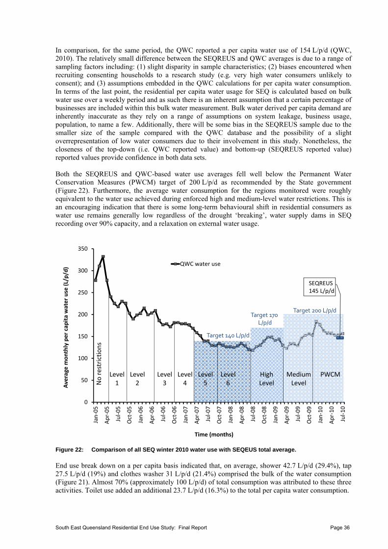
In comparison, for the same period, the QWC reported a per capita water use of 154 L/p/d (QWC, 2010). The relatively small difference between the SEQREUS and QWC averages is due to a range of sampling factors including: (1) slight disparity in sample characteristics; (2) biases encountered when recruiting consenting households to a research study (e.g. very high water consumers unlikely to consent); and (3) assumptions embedded in the QWC calculations for per capita water consumption. In terms of the last point, the residential per capita water usage for SEQ is calculated based on bulk water use over a weekly period and as such there is an inherent assumption that a certain percentage of businesses are included within this bulk water measurement. Bulk water derived per capita demand are inherently inaccurate as they rely on a range of assumptions on system leakage, business usage, population, to name a few. Additionally, there will be some bias in the SEQREUS sample due to the smaller size of the sample compared with the QWC database and the possibility of a slight overrepresentation of low water consumers due to their involvement in this study. Nonetheless, the closeness of the top-down (i.e. QWC reported value) and bottom-up (SEQREUS reported value) reported values provide confidence in both data sets. Both the SEQREUS and QWC-based water use averages fell well below the Permanent Water Conservation Measures (PWCM) target of 200 L/p/d as recommended by the State government (Figure 22). Furthermore, the average water consumption for the regions monitored were roughly equivalent to the water use achieved during enforced high and medium-level water restrictions. This is an encouraging indication that there is some long-term behavioural shift in residential consumers as water use remains generally low regardless of the drought ‘breaking’, water supply dams in SEQ recording over 90% capacity, and a relaxation on external water usage.
0
50
100
150
200
250
300
350
Jan‐05
Apr‐05
Jul‐05
Oct‐05
Jan‐06
Apr‐06
Jul‐06
Oct‐06
Jan‐07
Apr‐07
Jul‐07
Oct‐07
Jan‐08
Apr‐08
Jul‐08
Oct‐08
Jan‐09
Apr‐09
Jul‐09
Oct‐09
Jan‐10
Apr‐10
Jul‐10
Average m
onthly per capita water use (L/p/d)
Time (months)
QWC water use
SEQREUS145 L/p/d
No restrictions
Level1
Level2
Level3
Level4
Level5
Level6
HighLevel
MediumLevel
PWCM
Target 140 L/p/d
Target 170L/p/d
Target 200 L/p/d
Figure 22: Comparison of all SEQ winter 2010 water use with SEQEUS total average. End use break down on a per capita basis indicated that, on average, shower 42.7 L/p/d (29.4%), tap 27.5 L/p/d (19%) and clothes washer 31 L/p/d (21.4%) comprised the bulk of the water consumption (Figure 21). Almost 70% (approximately 100 L/p/d) of total consumption was attributed to these three activities. Toilet use added an additional 23.7 L/p/d (16.3%) to the total per capita water consumption.
South East Queensland Residential End Use Study: Final Report Page 36

Interestingly, water consumption for irrigation and general outdoor purposes was found to be low, at an average of only 7 L/p/d, which is less than 5% of total consumption (Figure 21). This low irrigation value indicates that the very high restrictions incurred in 2006 and 2007, may have had a lasting influence on the way people view their lawn and gardens.
The individual household per capita water consumption activity break down is shown in Figure 23. Water end use breakdowns varied substantially across (and within) the regions examined. This variation is a reflection of several factors, including family size and composition, socio-demographic factors and climate. In all homes measured, there was water use from toilet, clothes washer, taps and showers. The remaining end uses analysed, namely leaks, dishwasher, irrigation and bath tub, were reported in some but not all of the homes.
0
100
200
300
400
500
600
700
Household W
ater Consumption (L/p/d)
Household ID
Irrigation Bath Tap
Dish Washer Shower Clothes Washer
Toilet Leak
Figure 23: Household per capita winter 2010 consumption (L/p/d) activity break down. Typically, the homes that used the most water had a disproportionately high contribution from irrigation. This is shown by the strong correlation observed between total household water use and irrigation (Figure 24). The frequency distribution for irrigation (Figure 24) indicates that half the homes monitored did not register any irrigation use during the period of analysis. The lack of irrigation could be attributed to the winter season where outdoor watering is usually lower than in the hotter summer climate. Additionally, as discussed previously, there may be a tendency for lower external watering to occur due to the change in behaviours as a result of the water restrictions adhered to during the relatively recent drought period. However, 20% of the homes that did irrigate (or use water for external purposes) contributed to over 80% of total irrigation water use at an average of 30 L/p/d. This pareto effect has been observed in other residential water use studies (Willis et al., 2009b; Turner et al., 2009) and is a good example of why water restriction policy targets outdoor use to reduce residential demand (Barrett et al., 2009; Inman and Jeffrey, 2006; Kenney et al., 2008).
South East Queensland Residential End Use Study: Final Report Page 37
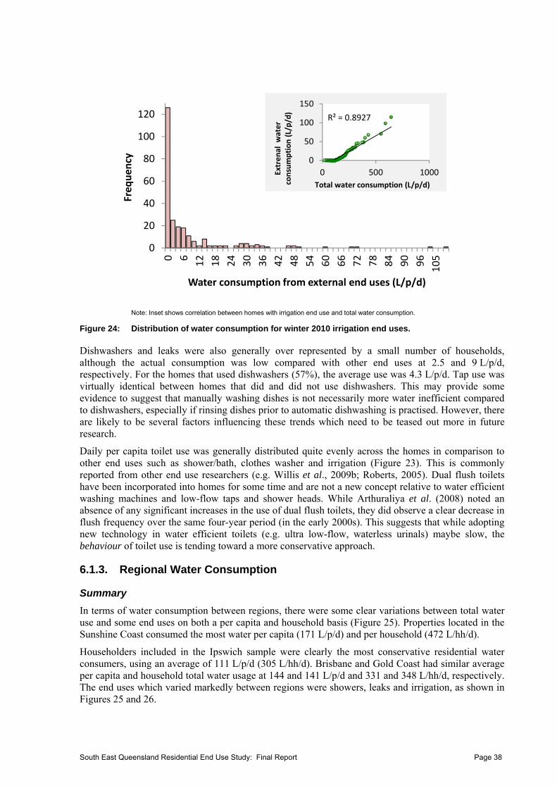
0
20
40
60
80
100
120
0 6
12
18
24
30
36
42
48
54
60
66
72
78
84
90
96
105
Freq
uen
cy
Water consumption from external end uses (L/p/d)
R² = 0.8927
0
50
100
150
0 500 1000Extrenal w
ater
consumption (L/p/d)
Total water consumption (L/p/d)
Note: Inset shows correlation between homes with irrigation end use and total water consumption.
Figure 24: Distribution of water consumption for winter 2010 irrigation end uses. Dishwashers and leaks were also generally over represented by a small number of households, although the actual consumption was low compared with other end uses at 2.5 and 9 L/p/d, respectively. For the homes that used dishwashers (57%), the average use was 4.3 L/p/d. Tap use was virtually identical between homes that did and did not use dishwashers. This may provide some evidence to suggest that manually washing dishes is not necessarily more water inefficient compared to dishwashers, especially if rinsing dishes prior to automatic dishwashing is practised. However, there are likely to be several factors influencing these trends which need to be teased out more in future research.
Daily per capita toilet use was generally distributed quite evenly across the homes in comparison to other end uses such as shower/bath, clothes washer and irrigation (Figure 23). This is commonly reported from other end use researchers (e.g. Willis et al., 2009b; Roberts, 2005). Dual flush toilets have been incorporated into homes for some time and are not a new concept relative to water efficient washing machines and low-flow taps and shower heads. While Arthuraliya et al. (2008) noted an absence of any significant increases in the use of dual flush toilets, they did observe a clear decrease in flush frequency over the same four-year period (in the early 2000s). This suggests that while adopting new technology in water efficient toilets (e.g. ultra low-flow, waterless urinals) maybe slow, the behaviour of toilet use is tending toward a more conservative approach.
6.1.3. Regional Water Consumption
Summary
In terms of water consumption between regions, there were some clear variations between total water use and some end uses on both a per capita and household basis (Figure 25). Properties located in the Sunshine Coast consumed the most water per capita (171 L/p/d) and per household (472 L/hh/d).
Householders included in the Ipswich sample were clearly the most conservative residential water consumers, using an average of 111 L/p/d (305 L/hh/d). Brisbane and Gold Coast had similar average per capita and household total water usage at 144 and 141 L/p/d and 331 and 348 L/hh/d, respectively. The end uses which varied markedly between regions were showers, leaks and irrigation, as shown in Figures 25 and 26.
South East Queensland Residential End Use Study: Final Report Page 38
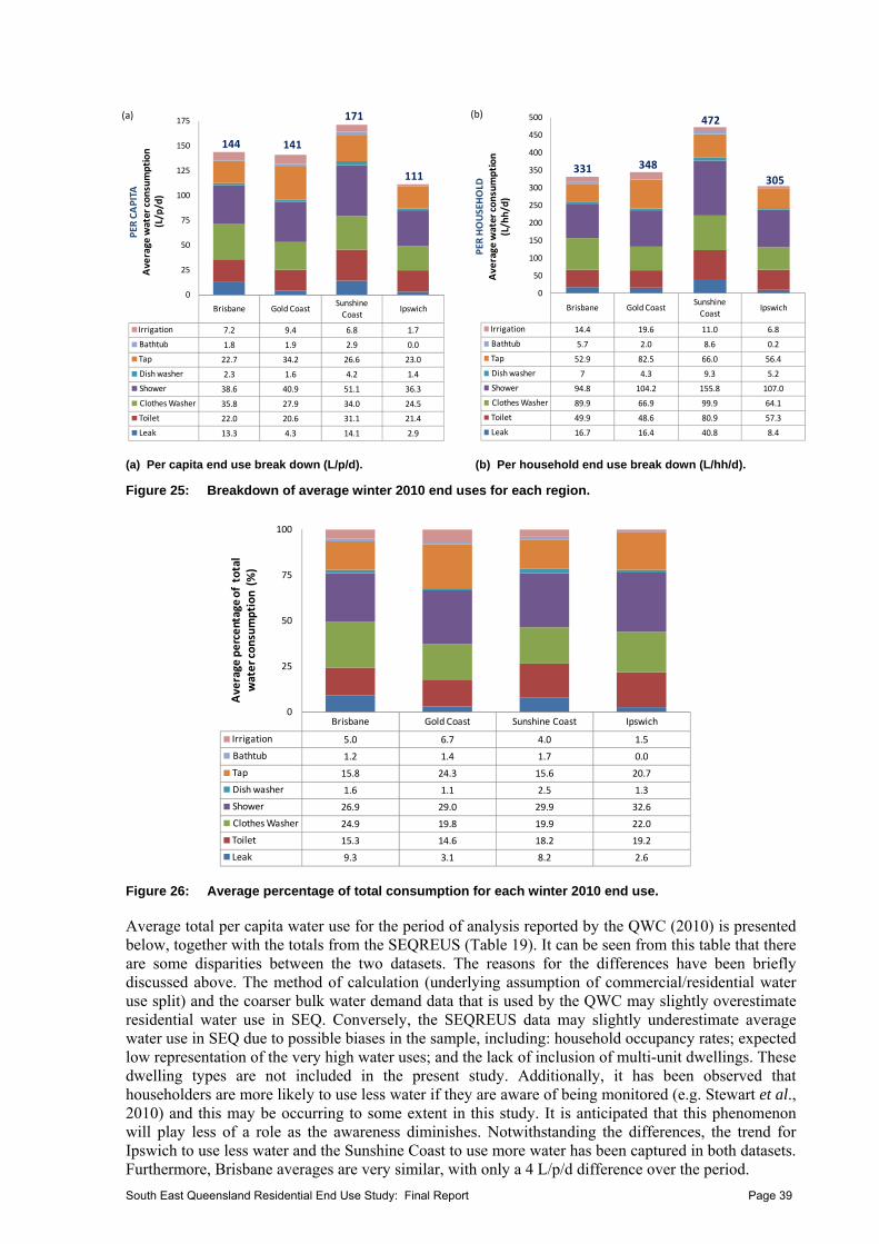
(a) Per capita end use break down (L/p/d). (b) Per household end use break down (L/hh/d).
Figure 25: Breakdown of average winter 2010 end uses for each region.
Figure 26: Average percentage of total consumption for each winter 2010 end use.
Average total per capita water use for the period of analysis reported by the QWC (2010) is presented below, together with the totals from the SEQREUS (Table 19). It can be seen from this table that there are some disparities between the two datasets. The reasons for the differences have been briefly discussed above. The method of calculation (underlying assumption of commercial/residential water use split) and the coarser bulk water demand data that is used by the QWC may slightly overestimate residential water use in SEQ. Conversely, the SEQREUS data may slightly underestimate average water use in SEQ due to possible biases in the sample, including: household occupancy rates; expected low representation of the very high water uses; and the lack of inclusion of multi-unit dwellings. These dwelling types are not included in the present study. Additionally, it has been observed that householders are more likely to use less water if they are aware of being monitored (e.g. Stewart et al., 2010) and this may be occurring to some extent in this study. It is anticipated that this phenomenon will play less of a role as the awareness diminishes. Notwithstanding the differences, the trend for Ipswich to use less water and the Sunshine Coast to use more water has been captured in both datasets. Furthermore, Brisbane averages are very similar, with only a 4 L/p/d difference over the period.
Brisbane Gold CoastSunshine Coast
Ipswich
Irrigation 7.2 9.4 6.8 1.7
Bathtub 1.8 1.9 2.9 0.0
Tap 22.7 34.2 26.6 23.0
Dish washer 2.3 1.6 4.2 1.4
Shower 38.6 40.9 51.1 36.3
Clothes Washer 35.8 27.9 34.0 24.5
Toilet 22.0 20.6 31.1 21.4
Leak 13.3 4.3 14.1 2.9
0
25
50
75
100
125
150
175
PER
CAPITA
Average water consumption
(L/p/d)
144
171
111
141
(a)
Brisbane Gold CoastSunshine
CoastIpswich
Irrigation 14.4 19.6 11.0 6.8
Bathtub 5.7 2.0 8.6 0.2
Tap 52.9 82.5 66.0 56.4
Dish washer 7 4.3 9.3 5.2
Shower 94.8 104.2 155.8 107.0
Clothes Washer 89.9 66.9 99.9 64.1
Toilet 49.9 48.6 80.9 57.3
Leak 16.7 16.4 40.8 8.4
0
50
100
150
200
250
300
350
400
450
500
PER
HOUSEHOLD
Average water consumption
(L/hh/d)
331
472
305
348
(b)
Brisbane Gold Coast Sunshine Coast Ipswich
Irrigation 5.0 6.7 4.0 1.5
Bathtub 1.2 1.4 1.7 0.0
Tap 15.8 24.3 15.6 20.7
Dish washer 1.6 1.1 2.5 1.3
Shower 26.9 29.0 29.9 32.6
Clothes Washer 24.9 19.8 19.9 22.0
Toilet 15.3 14.6 18.2 19.2
Leak 9.3 3.1 8.2 2.6
0
25
50
75
100
Average percentage of total
water consumption (%)
South East Queensland Residential End Use Study: Final Report Page 39
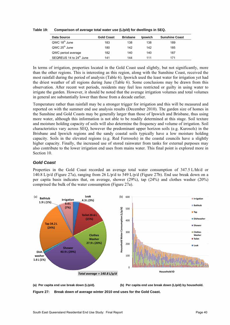
Table 19: Comparison of average total water use (L/p/d) for dwellings in SEQ.
Data Source Gold Coast Brisbane Ipswich Sunshine Coast
QWC 18th June 183 138 138 189
QWC 25th June 180 142 142 185
QWC period average 182 140 140 187
SEQREUS 14 to 24th June 141 144 111 171
In terms of irrigation, properties located in the Gold Coast used slightly, but not significantly, more than the other regions. This is interesting as this region, along with the Sunshine Coast, received the most rainfall during the period of analysis (Table 6). Ipswich used the least water for irrigation yet had the driest weather of all regions during June (Table 6). Some conclusions may be drawn from this observation. After recent wet periods, residents may feel less restricted or guilty in using water to irrigate the garden. However, it should be noted that the average irrigation volumes and total volumes in general are substantially lower than those from a decade earlier.
Temperature rather than rainfall may be a stronger trigger for irrigation and this will be measured and reported on with the summer end use analysis results (December 2010). The garden size of homes in the Sunshine and Gold Coasts may be generally larger than those of Ipswich and Brisbane, thus using more water, although this information is not able to be readily determined at this stage. Soil texture and moisture holding capacity of soils will also determine the frequency and volume of irrigation. Soil characteristics vary across SEQ, however the predominant upper horizon soils (e.g. Kurosols) in the Brisbane and Ipswich regions and the sandy coastal soils typically have a low moisture holding capacity. Soils in the elevated regions (e.g. Red Ferrosols) in the coastal councils have a slightly higher capacity. Finally, the increased use of stored rainwater from tanks for external purposes may also contribute to the lower irrigation end uses from mains water. This final point is explored more in Section 10.
Gold Coast
Properties in the Gold Coast recorded an average total water consumption of 347.5 L/hh/d or 140.8 L/p/d (Figure 27a), ranging from 26 L/p/d to 549 L/p/d (Figure 27b). End use break down on a per capita basis indicates that, on average, shower (29%), tap (24%) and clothes washer (20%) comprised the bulk of the water consumption (Figure 27a).
(a) Per capita end use break down (L/p/d) (b) Per capita end use break down (L/p/d) by household
0
100
200
300
400
500
600
Household W
ater Consumption (L/p/d)
Household ID
Irrigation
Bathtub
Tap
Dishwasher
Shower
Clothes Washer
Toilet
Leak
(b)Leak4.3 L (3%)
Toilet 20.6 L (15%)
Clothes Washer
27.9 L (20%)
Shower 40.9 L (29%)Dish
washer1.6 L (1%)
Tap 34.2 L(24%)
Bathtub1.9 L (1%)
Irrigation9.4 L (7%)
Total average = 140.8 L/p/d
(a)
(a) Per capita end use break down (L/p/d). (b) Per capita end use break down (L/p/d) by household.
Figure 27: Break down of average winter 2010 end uses for the Gold Coast.
South East Queensland Residential End Use Study: Final Report Page 40

Irrigation contributed an average of 9.4 L/p/d or 7% of total water use. The homes that used the most water had a disproportionately high contribution from irrigation (Figure 27b). This is consistent across all regions examined. Water used for clothes washing and showers was markedly varied across the sample and may reflect the mix of household types (single, family, pensioners) that were present in this region. Data from Table 7 suggests that both small and large families with young children were fairly evenly represented compared to the other regions.
Brisbane
Average household consumption in Brisbane was 331.4 L/hh/d, resulting in a per capita consumption average of 143.8 L/p/d (Figure 28). End use break down on a per capita basis indicates that, once again, shower (26.9%), clothes washer (24.9%) and tap (15.8%) comprised the bulk of the water consumption (Figure 28a), contributing over 65% (97 L/p/d) of daily usage. There was an association between the number of young children in the home and clothes washing and showering. The Brisbane sample had the youngest average age of children (2.7 years) and the highest consumption for water resulting from clothes washing (Figure 26).
The Brisbane total amount of daily per capita usage attributed to leaks was the second highest across the regions at 13.3 L/p/d representing 9.3% of total household water use (Figure 26 and Figure 28a). However, this result was skewed by extraordinarily high leak usage attributed to two homes, with one household showing average daily consumption from leaks at over 500 L/p/d (Figure 28b). For the average householder, the percentage attributed to leaks was much less at 4.4 L/p/d (3% of total water use). It is necessary to include these high leak homes as they are not outliers, rather they represent a small number of homes (usually 3-5% of dwelling stock) having very high leakage rates and this is typical of a ‘normal’ sample of households (Britton et al., 2009).
Irrigation in the Brisbane region was 5% of total daily usage, or 7.2 L/p/d. This figure was over-represented in some households (Figure 28b). It was noted during the analysis that people who reported that they irrigate their gardens usually did so using a constant and medium flow rate with the event lasting between 15 minutes to one hour on average.
Leak 13.3 L/p/d(9.3%)
Toilet 22 Lp/d (15.3%)
Clothes Washer 35.8 L/p/d (24.9%)
Shower 38.6 L/p d (26.9%)
Dish washer 2.3 L/p/d(1.6%)
Tap 22.7 L/p/d (15.8%)
Bathtub 1.8 L/p/d (1.2%)
Irrigation 7.2 L/p/d (5%)
Total average = 143.8 L/p/d
(a)
0
100
200
300
400
500
600
700
Household W
ater Consumption (L/p/d)
Household ID
Irrigation
Bathtub
Tap
Dishwasher
Shower
Clothes Washer
Toilet
Leak
(b)
(a) Per capita end use break down (L/p/d). (b) Per capita end use break down (L/p/d) by household.
Figure 28: Break down of average winter 2010 end uses for Brisbane.
Ipswich
The period of analysis in the Ipswich region showed an average household consumption of 305.4 L/hh/day. This resulted in a low per capita figure of 111.2 L/p/d (Figure 29a), nearly half of the QWC Permanent Water Conservation Measures target of 200 L/p/d. Per capita total water use ranged from 283 to 20 L/p/d (Figure 29b). The low per capita use (20 L/p/d) measured for one home was a result of frequent absences of the sole occupant of the property.
South East Queensland Residential End Use Study: Final Report Page 41
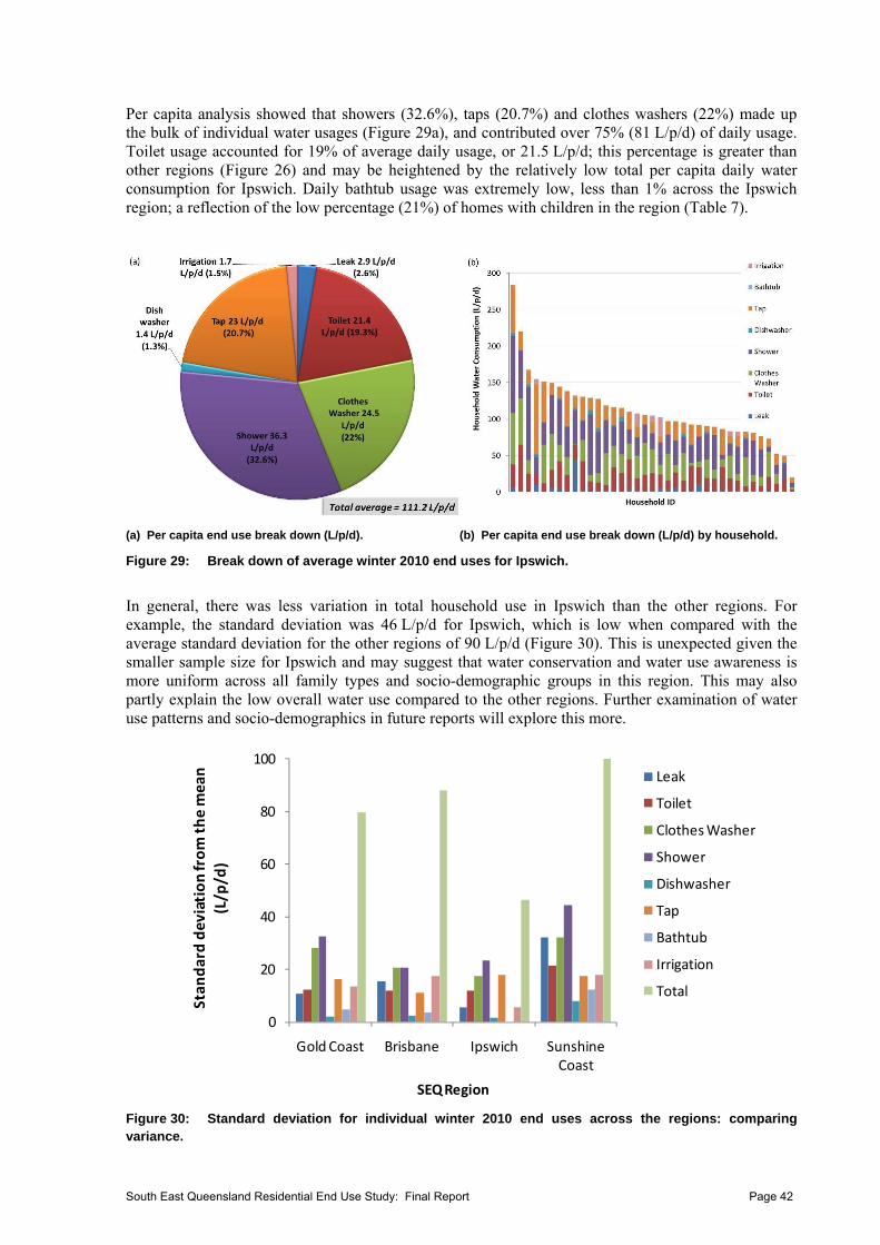
Per capita analysis showed that showers (32.6%), taps (20.7%) and clothes washers (22%) made up the bulk of individual water usages (Figure 29a), and contributed over 75% (81 L/p/d) of daily usage. Toilet usage accounted for 19% of average daily usage, or 21.5 L/p/d; this percentage is greater than other regions (Figure 26) and may be heightened by the relatively low total per capita daily water consumption for Ipswich. Daily bathtub usage was extremely low, less than 1% across the Ipswich region; a reflection of the low percentage (21%) of homes with children in the region (Table 7).
(a) Per capita end use break down (L/p/d). (b) Per capita end use break down (L/p/d) by household.
Figure 29: Break down of average winter 2010 end uses for Ipswich.
In general, there was less variation in total household use in Ipswich than the other regions. For example, the standard deviation was 46 L/p/d for Ipswich, which is low when compared with the average standard deviation for the other regions of 90 L/p/d (Figure 30). This is unexpected given the smaller sample size for Ipswich and may suggest that water conservation and water use awareness is more uniform across all family types and socio-demographic groups in this region. This may also partly explain the low overall water use compared to the other regions. Further examination of water use patterns and socio-demographics in future reports will explore this more.
0
20
40
60
80
100
Gold Coast Brisbane Ipswich Sunshine Coast
Standard deviation from the mean
(L/p/d)
SEQ Region
Leak
Toilet
Clothes Washer
Shower
Dishwasher
Tap
Bathtub
Irrigation
Total
Figure 30: Standard deviation for individual winter 2010 end uses across the regions: comparing variance.
South East Queensland Residential End Use Study: Final Report Page 42
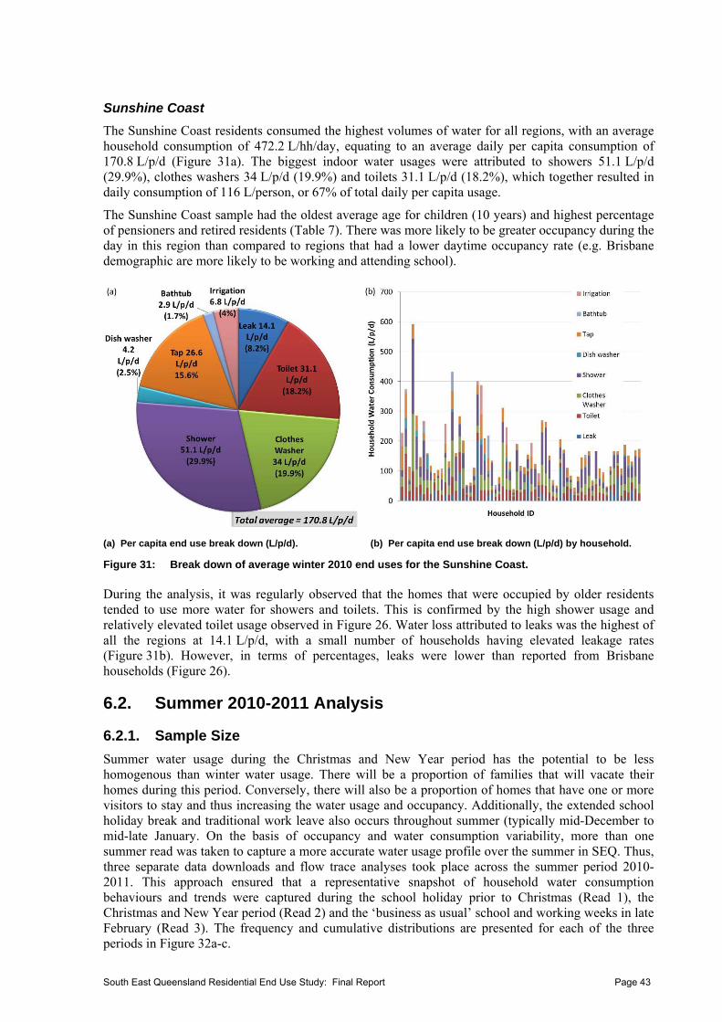
Sunshine Coast
The Sunshine Coast residents consumed the highest volumes of water for all regions, with an average household consumption of 472.2 L/hh/day, equating to an average daily per capita consumption of 170.8 L/p/d (Figure 31a). The biggest indoor water usages were attributed to showers 51.1 L/p/d (29.9%), clothes washers 34 L/p/d (19.9%) and toilets 31.1 L/p/d (18.2%), which together resulted in daily consumption of 116 L/person, or 67% of total daily per capita usage.
The Sunshine Coast sample had the oldest average age for children (10 years) and highest percentage of pensioners and retired residents (Table 7). There was more likely to be greater occupancy during the day in this region than compared to regions that had a lower daytime occupancy rate (e.g. Brisbane demographic are more likely to be working and attending school).
(a) Per capita end use break down (L/p/d). (b) Per capita end use break down (L/p/d) by household.
Figure 31: Break down of average winter 2010 end uses for the Sunshine Coast. During the analysis, it was regularly observed that the homes that were occupied by older residents tended to use more water for showers and toilets. This is confirmed by the high shower usage and relatively elevated toilet usage observed in Figure 26. Water loss attributed to leaks was the highest of all the regions at 14.1 L/p/d, with a small number of households having elevated leakage rates (Figure 31b). However, in terms of percentages, leaks were lower than reported from Brisbane households (Figure 26).
6.2. Summer 2010-2011 Analysis
6.2.1. Sample Size
Summer water usage during the Christmas and New Year period has the potential to be less homogenous than winter water usage. There will be a proportion of families that will vacate their homes during this period. Conversely, there will also be a proportion of homes that have one or more visitors to stay and thus increasing the water usage and occupancy. Additionally, the extended school holiday break and traditional work leave also occurs throughout summer (typically mid-December to mid-late January. On the basis of occupancy and water consumption variability, more than one summer read was taken to capture a more accurate water usage profile over the summer in SEQ. Thus, three separate data downloads and flow trace analyses took place across the summer period 2010-2011. This approach ensured that a representative snapshot of household water consumption behaviours and trends were captured during the school holiday prior to Christmas (Read 1), the Christmas and New Year period (Read 2) and the ‘business as usual’ school and working weeks in late February (Read 3). The frequency and cumulative distributions are presented for each of the three periods in Figure 32a-c.
South East Queensland Residential End Use Study: Final Report Page 43
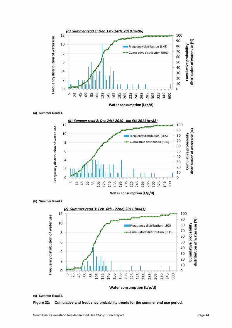
0
10
20
30
40
50
60
70
80
90
100
0
2
4
6
8
10
12
5
25
45
65
85
105
125
145
165
185
205
225
245
265
285
305
325
345
600
Cumulative
probability
distribution of w
ater use (%
)
Frequency distribution of w
ater use
Water consumption (L/p/d)
Frequency distribution (LHS)
Cumulative distribution (RHS)
(a) Summer read 1: Dec 1st ‐ 14th, 2010 (n=96)
(a) Summer Read 1.
0
10
20
30
40
50
60
70
80
90
100
0
2
4
6
8
10
12
5
25
45
65
85
105
125
145
165
185
205
225
245
265
285
305
325
345
600
Cumulative
probability
distribution of w
ater use (%
)
Frequency distribution of w
ater use
Water consumption (L/p/d)
Frequency distribution (LHS)
Cumulative distribution (RHS)
(b) Summer read 2: Dec 24th 2010 ‐ Jan 6th 2011 (n=82)
(b) Summer Read 2.
0
10
20
30
40
50
60
70
80
90
100
0
2
4
6
8
10
12
5
25
45
65
85
105
125
145
165
185
205
225
245
265
285
305
325
345
600
Cumulative probab
ility
distribution of water use (%)
Frequency distribution of water use
Water consumption (L/p/d)
Frequency distribution (LHS)
Cumulative distribution (RHS)
(c) Summer read 3: Feb 6th ‐ 22nd, 2011 (n=41)
(c) Summer Read 3.
Figure 32: Cumulative and frequency probability trends for the summer end use period.
South East Queensland Residential End Use Study: Final Report Page 44
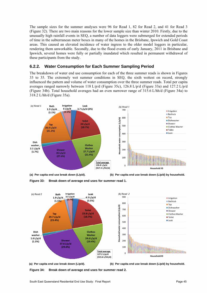
The sample sizes for the summer analyses were 96 for Read 1, 82 for Read 2, and 41 for Read 3 (Figure 32). There are two main reasons for the lower sample size than winter 2010. Firstly, due to the unusually high rainfall events in SEQ, a number of data loggers were submerged for extended periods of time in the subterranean meter boxes in many of the homes in the Brisbane, Ipswich and Gold Coast areas. This caused an elevated incidence of water ingress to the older model loggers in particular, rendering them unworkable. Secondly, due to the flood events of early January, 2011 in Brisbane and Ipswich, several homes were fully or partially inundated which resulted in permanent withdrawal of these participants from the study.
6.2.2. Water Consumption for Each Summer Sampling Period
The breakdown of water end use consumption for each of the three summer reads is shown in Figures 33 to 35. The extremely wet summer conditions in SEQ, the sixth wettest on record, strongly influenced the pattern and volume of water consumption over the three summer reads. Total per capita averages ranged narrowly between 118 L/p/d (Figure 35c), 126.8 L/p/d (Figure 33a) and 127.2 L/p/d (Figure 34b). Total household averages had an even narrower range of 315.6 L/hh/d (Figure 34a) to 318.2 L/hh/d (Figure 35a).
(a) Per capita end use break down (L/p/d). (b) Per capita end use break down (L/p/d) by household.
Figure 33: Break down of average end uses for summer read 1.
Leak4.5 L/p/d (3.5%)
Toilet23.8 L/p/d (18.7%)
Clothes Washer
24.6 L/p/d (19.4%)Shower
37.6 L/p/d (29.6%)
Dish washer1.6 L/p/d(1.3%)
Tap29.7 L/p/d (23.4%)
Bath1.9 L/p/d (1.5%)
Irrigation3.5 L/p/d (2.7%)
Total average 127.2 L/p/d(315.6 L/hh/d)
(a) Read 2
0
100
200
300
400
500
600
700
800
900
Household water consumption (L/p/d)
Household ID
Irrigation
Bathtub
Tap
Dishwasher
Shower
Clothes Washer
Toilet
Leak
(b) Read 2
(a) Per capita end use break down (L/p/d). (b) Per capita end use break down (L/p/d) by household.
Figure 34: Break down of average end uses for summer read 2.
South East Queensland Residential End Use Study: Final Report Page 45
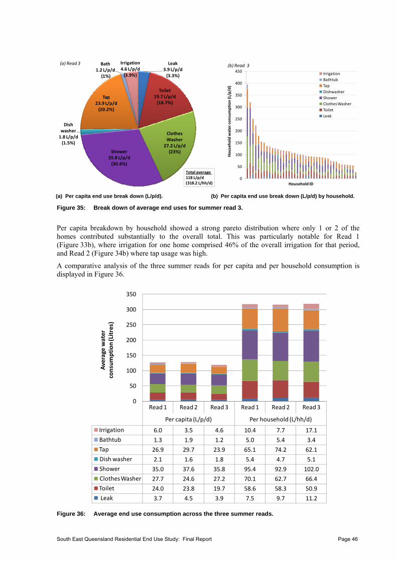
Leak3.9 L/p/d (3.3%)
Toilet19.7 L/p/d (16.7%)
Clothes Washer
27.2 L/p/d (23%)Shower
35.8 L/p/d (30.4%)
Dish washer1.8 L/p/d(1.5%)
Tap23.9 L/p/d (20.2%)
Bath1.2 L/p/d
(1%)
Irrigation4.6 L/p/d (3.9%)
Total average 118 L/p/d(318.2 L/hh/d)
(a) Read 3
0
50
100
150
200
250
300
350
400
450
Household water consumption (L/p/d)
Household ID
Irrigation
Bathtub
Tap
Dishwasher
Shower
Clothes Washer
Toilet
Leak
(b) Read 3
(a) Per capita end use break down (L/p/d). (b) Per capita end use break down (L/p/d) by household.
Figure 35: Break down of average end uses for summer read 3.
Per capita breakdown by household showed a strong pareto distribution where only 1 or 2 of the homes contributed substantially to the overall total. This was particularly notable for Read 1 (Figure 33b), where irrigation for one home comprised 46% of the overall irrigation for that period, and Read 2 (Figure 34b) where tap usage was high.
A comparative analysis of the three summer reads for per capita and per household consumption is displayed in Figure 36.
Read 1 Read 2 Read 3 Read 1 Read 2 Read 3
Per capita (L/p/d) Per household (L/hh/d)
Irrigation 6.0 3.5 4.6 10.4 7.7 17.1
Bathtub 1.3 1.9 1.2 5.0 5.4 3.4
Tap 26.9 29.7 23.9 65.1 74.2 62.1
Dish washer 2.1 1.6 1.8 5.4 4.7 5.1
Shower 35.0 37.6 35.8 95.4 92.9 102.0
Clothes Washer 27.7 24.6 27.2 70.1 62.7 66.4
Toilet 24.0 23.8 19.7 58.6 58.3 50.9
Leak 3.7 4.5 3.9 7.5 9.7 11.2
0
50
100
150
200
250
300
350
Average water
consumption (Litres)
Figure 36: Average end use consumption across the three summer reads.
South East Queensland Residential End Use Study: Final Report Page 46
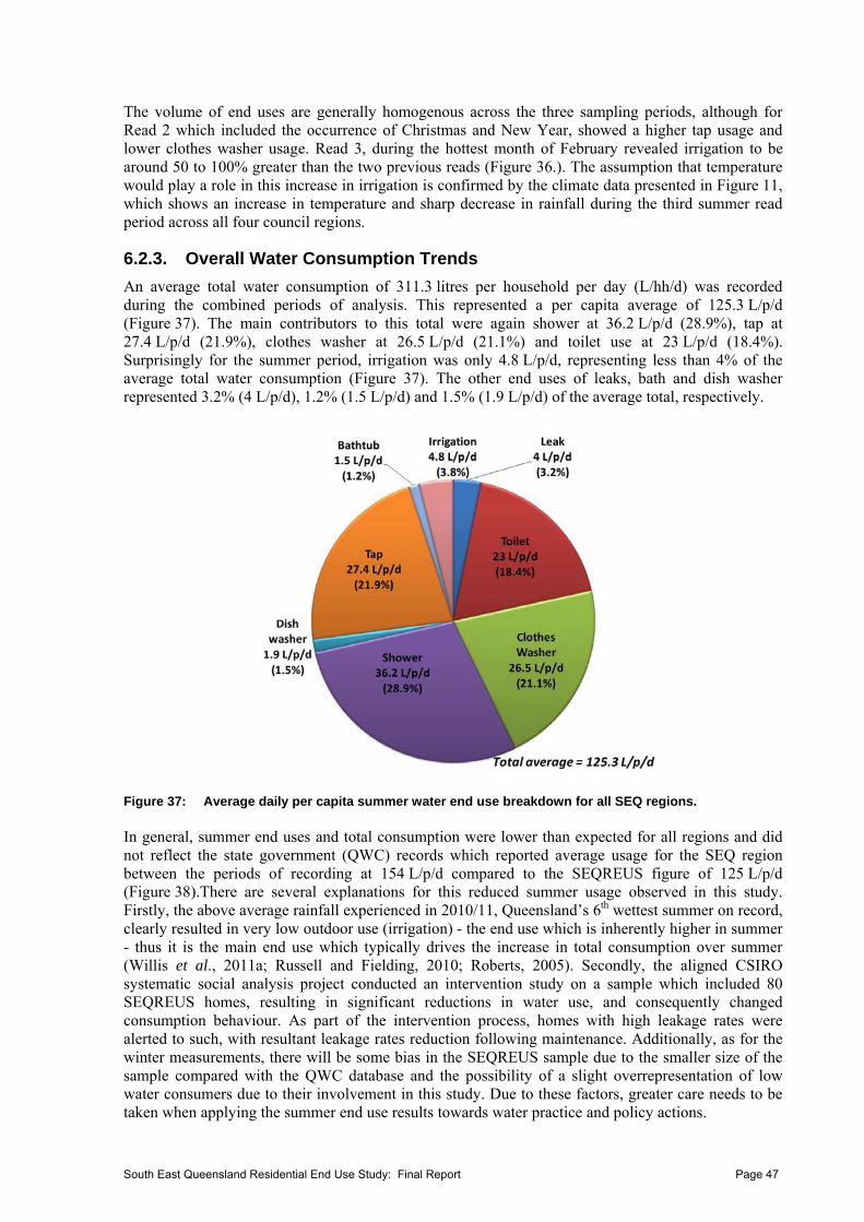
The volume of end uses are generally homogenous across the three sampling periods, although for Read 2 which included the occurrence of Christmas and New Year, showed a higher tap usage and lower clothes washer usage. Read 3, during the hottest month of February revealed irrigation to be around 50 to 100% greater than the two previous reads (Figure 36.). The assumption that temperature would play a role in this increase in irrigation is confirmed by the climate data presented in Figure 11, which shows an increase in temperature and sharp decrease in rainfall during the third summer read period across all four council regions.
6.2.3. Overall Water Consumption Trends
An average total water consumption of 311.3 litres per household per day (L/hh/d) was recorded during the combined periods of analysis. This represented a per capita average of 125.3 L/p/d (Figure 37). The main contributors to this total were again shower at 36.2 L/p/d (28.9%), tap at 27.4 L/p/d (21.9%), clothes washer at 26.5 L/p/d (21.1%) and toilet use at 23 L/p/d (18.4%). Surprisingly for the summer period, irrigation was only 4.8 L/p/d, representing less than 4% of the average total water consumption (Figure 37). The other end uses of leaks, bath and dish washer represented 3.2% (4 L/p/d), 1.2% (1.5 L/p/d) and 1.5% (1.9 L/p/d) of the average total, respectively. Figure 37: Average daily per capita summer water end use breakdown for all SEQ regions. In general, summer end uses and total consumption were lower than expected for all regions and did not reflect the state government (QWC) records which reported average usage for the SEQ region between the periods of recording at 154 L/p/d compared to the SEQREUS figure of 125 L/p/d (Figure 38).There are several explanations for this reduced summer usage observed in this study. Firstly, the above average rainfall experienced in 2010/11, Queensland’s 6th wettest summer on record, clearly resulted in very low outdoor use (irrigation) - the end use which is inherently higher in summer - thus it is the main end use which typically drives the increase in total consumption over summer (Willis et al., 2011a; Russell and Fielding, 2010; Roberts, 2005). Secondly, the aligned CSIRO systematic social analysis project conducted an intervention study on a sample which included 80 SEQREUS homes, resulting in significant reductions in water use, and consequently changed consumption behaviour. As part of the intervention process, homes with high leakage rates were alerted to such, with resultant leakage rates reduction following maintenance. Additionally, as for the winter measurements, there will be some bias in the SEQREUS sample due to the smaller size of the sample compared with the QWC database and the possibility of a slight overrepresentation of low water consumers due to their involvement in this study. Due to these factors, greater care needs to be taken when applying the summer end use results towards water practice and policy actions.
South East Queensland Residential End Use Study: Final Report Page 47

Figure 38: Comparison of all SEQ summer 2010-11 water use with SEQREUS total average. The household per capita water consumption activity break down is shown in Figure 39. As for winter 2010, in all homes measured there was water use from toilet, clothes washer, taps and showers. The remaining end uses analysed: leaks, dishwasher, irrigation and bath tub, were reported in some but not all of the homes. Similarly to winter 2010 results, a pareto-type distribution was observed where less than 3% of the homes contributed to over 10% of the total water usage (Figure 39). Extreme water usage for two homes (e.g. 785 and 655 L/p/d) which represented between five and six times the average, were driven not only by irrigation end use, but also by tap and shower.
0
100
200
300
400
500
600
700
800
Household water consumption (L/p/d)
Household ID
Irrigation Bath Tap Dishwasher
Shower Clothes Washer Toilet Leak
Figure 39: Household per capita summer consumption (L/p/d) activity break down.
South East Queensland Residential End Use Study: Final Report Page 48
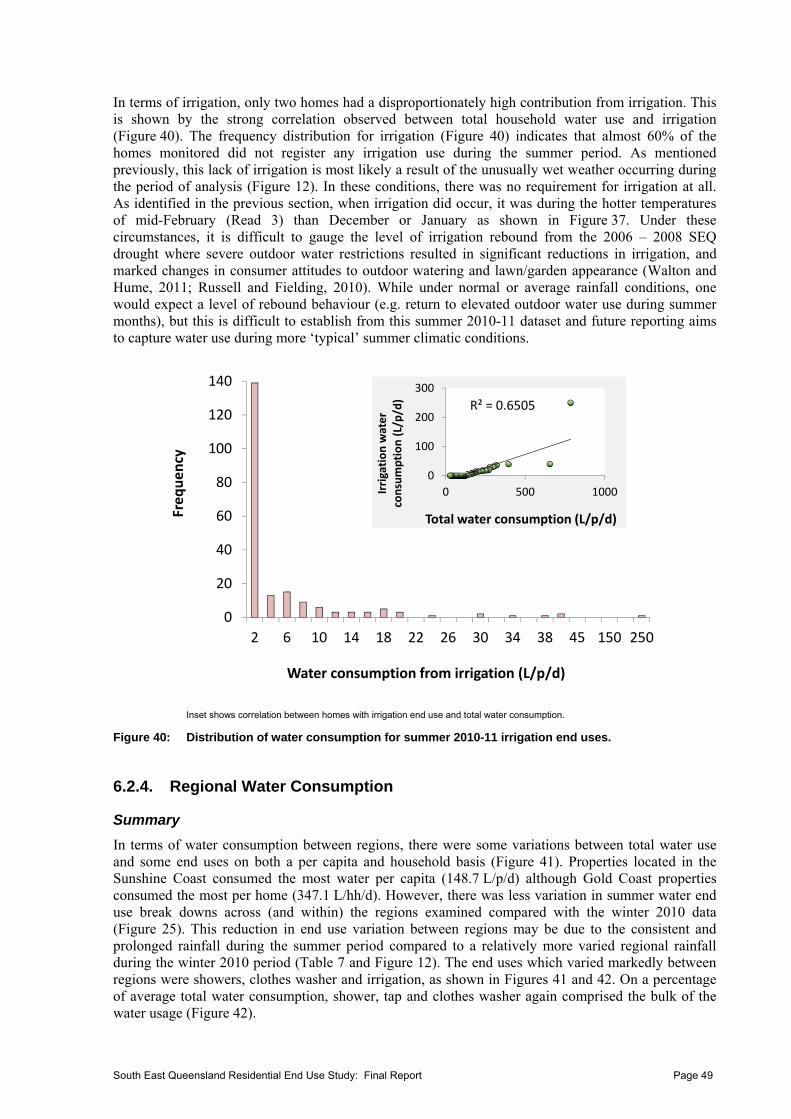
In terms of irrigation, only two homes had a disproportionately high contribution from irrigation. This is shown by the strong correlation observed between total household water use and irrigation (Figure 40). The frequency distribution for irrigation (Figure 40) indicates that almost 60% of the homes monitored did not register any irrigation use during the summer period. As mentioned previously, this lack of irrigation is most likely a result of the unusually wet weather occurring during the period of analysis (Figure 12). In these conditions, there was no requirement for irrigation at all. As identified in the previous section, when irrigation did occur, it was during the hotter temperatures of mid-February (Read 3) than December or January as shown in Figure 37. Under these circumstances, it is difficult to gauge the level of irrigation rebound from the 2006 – 2008 SEQ drought where severe outdoor water restrictions resulted in significant reductions in irrigation, and marked changes in consumer attitudes to outdoor watering and lawn/garden appearance (Walton and Hume, 2011; Russell and Fielding, 2010). While under normal or average rainfall conditions, one would expect a level of rebound behaviour (e.g. return to elevated outdoor water use during summer months), but this is difficult to establish from this summer 2010-11 dataset and future reporting aims to capture water use during more ‘typical’ summer climatic conditions.
0
20
40
60
80
100
120
140
2 6 10 14 18 22 26 30 34 38 45 150 250
Frequency
Water consumption from irrigation (L/p/d)
R² = 0.6505
0
100
200
300
0 500 1000Irrigation water
consumption (L/p/d)
Total water consumption (L/p/d)
Inset shows correlation between homes with irrigation end use and total water consumption.
Figure 40: Distribution of water consumption for summer 2010-11 irrigation end uses.
6.2.4. Regional Water Consumption
Summary
In terms of water consumption between regions, there were some variations between total water use and some end uses on both a per capita and household basis (Figure 41). Properties located in the Sunshine Coast consumed the most water per capita (148.7 L/p/d) although Gold Coast properties consumed the most per home (347.1 L/hh/d). However, there was less variation in summer water end use break downs across (and within) the regions examined compared with the winter 2010 data (Figure 25). This reduction in end use variation between regions may be due to the consistent and prolonged rainfall during the summer period compared to a relatively more varied regional rainfall during the winter 2010 period (Table 7 and Figure 12). The end uses which varied markedly between regions were showers, clothes washer and irrigation, as shown in Figures 41 and 42. On a percentage of average total water consumption, shower, tap and clothes washer again comprised the bulk of the water usage (Figure 42).
South East Queensland Residential End Use Study: Final Report Page 49
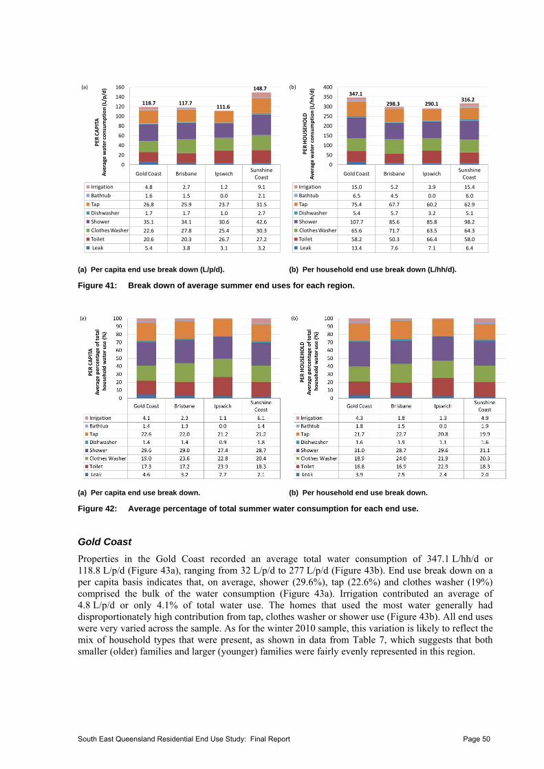
Gold Coast Brisbane IpswichSunshine Coast
Irrigation 4.8 2.7 1.2 9.1
Bathtub 1.6 1.5 0.0 2.1
Tap 26.8 25.9 23.7 31.5
Dishwasher 1.7 1.7 1.0 2.7
Shower 35.1 34.1 30.6 42.6
Clothes Washer 22.6 27.8 25.4 30.3
Toilet 20.6 20.3 26.7 27.2
Leak 5.4 3.8 3.1 3.2
0
20
40
60
80
100
120
140
160
PER
CAPITA
Average water consumption (L/p/d)
118.7
148.7
111.6117.7
(a)
Gold Coast Brisbane IpswichSunshine Coast
Irrigation 15.0 5.2 3.9 15.4
Bathtub 6.5 4.5 0.0 6.0
Tap 75.4 67.7 60.2 62.9
Dishwasher 5.4 5.7 3.2 5.1
Shower 107.7 85.6 85.8 98.2
Clothes Washer 65.6 71.7 63.5 64.3
Toilet 58.2 50.3 66.4 58.0
Leak 13.4 7.6 7.1 6.4
0
50
100
150
200
250
300
350
400
PER HOUSEHOLD
Average water consumption (L/hh/d)
347.1316.2
290.1298.3
(b)
(a) Per capita end use break down (L/p/d). (b) Per household end use break down (L/hh/d).
Figure 41: Break down of average summer end uses for each region.
(a) Per capita end use break down. (b) Per household end use break down.
Figure 42: Average percentage of total summer water consumption for each end use.
Gold Coast
Properties in the Gold Coast recorded an average total water consumption of 347.1 L/hh/d or 118.8 L/p/d (Figure 43a), ranging from 32 L/p/d to 277 L/p/d (Figure 43b). End use break down on a per capita basis indicates that, on average, shower (29.6%), tap (22.6%) and clothes washer (19%) comprised the bulk of the water consumption (Figure 43a). Irrigation contributed an average of 4.8 L/p/d or only 4.1% of total water use. The homes that used the most water generally had disproportionately high contribution from tap, clothes washer or shower use (Figure 43b). All end uses were very varied across the sample. As for the winter 2010 sample, this variation is likely to reflect the mix of household types that were present, as shown in data from Table 7, which suggests that both smaller (older) families and larger (younger) families were fairly evenly represented in this region.
South East Queensland Residential End Use Study: Final Report Page 50
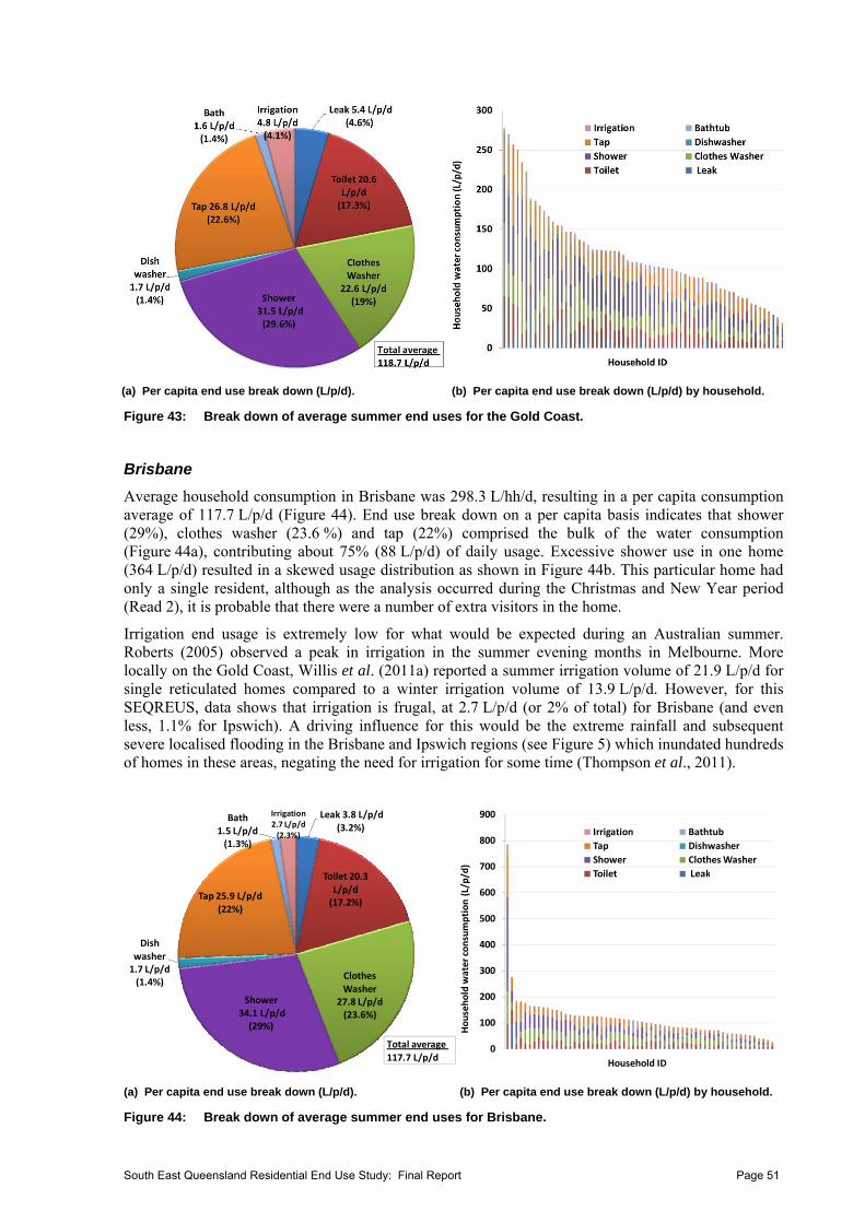
(a) Per capita end use break down (L/p/d). (b) Per capita end use break down (L/p/d) by household.
Figure 43: Break down of average summer end uses for the Gold Coast.
Brisbane
Average household consumption in Brisbane was 298.3 L/hh/d, resulting in a per capita consumption average of 117.7 L/p/d (Figure 44). End use break down on a per capita basis indicates that shower (29%), clothes washer (23.6 %) and tap (22%) comprised the bulk of the water consumption (Figure 44a), contributing about 75% (88 L/p/d) of daily usage. Excessive shower use in one home (364 L/p/d) resulted in a skewed usage distribution as shown in Figure 44b. This particular home had only a single resident, although as the analysis occurred during the Christmas and New Year period (Read 2), it is probable that there were a number of extra visitors in the home.
Irrigation end usage is extremely low for what would be expected during an Australian summer. Roberts (2005) observed a peak in irrigation in the summer evening months in Melbourne. More locally on the Gold Coast, Willis et al. (2011a) reported a summer irrigation volume of 21.9 L/p/d for single reticulated homes compared to a winter irrigation volume of 13.9 L/p/d. However, for this SEQREUS, data shows that irrigation is frugal, at 2.7 L/p/d (or 2% of total) for Brisbane (and even less, 1.1% for Ipswich). A driving influence for this would be the extreme rainfall and subsequent severe localised flooding in the Brisbane and Ipswich regions (see Figure 5) which inundated hundreds of homes in these areas, negating the need for irrigation for some time (Thompson et al., 2011).
Leak 3.8 L/p/d(3.2%)
Toilet 20.3
L/p/d(17.2%)
Clothes Washer
27.8 L/p/d(23.6%)
Shower 34.1 L/p/d(29%)
Dish
washer 1.7 L/p/d(1.4%)
Tap 25.9 L/p/d
(22%)
Bath 1.5 L/p/d(1.3%)
Irrigation 2.7 L/p/d(2.3%)
Total average
117.7 L/p/d0
100
200
300
400
500
600
700
800
900
Household water consumption (L/p/d)
Household ID
Irrigation Bathtub
Tap Dishwasher
Shower Clothes Washer
Toilet Leak
(a) Per capita end use break down (L/p/d). (b) Per capita end use break down (L/p/d) by household.
Figure 44: Break down of average summer end uses for Brisbane.
South East Queensland Residential End Use Study: Final Report Page 51
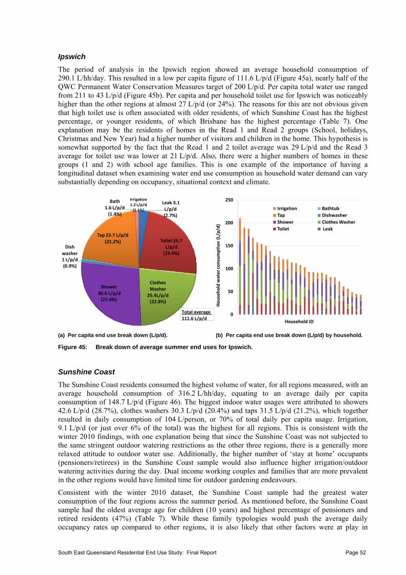
Ipswich
The period of analysis in the Ipswich region showed an average household consumption of 290.1 L/hh/day. This resulted in a low per capita figure of 111.6 L/p/d (Figure 45a), nearly half of the QWC Permanent Water Conservation Measures target of 200 L/p/d. Per capita total water use ranged from 211 to 43 L/p/d (Figure 45b). Per capita and per household toilet use for Ipswich was noticeably higher than the other regions at almost 27 L/p/d (or 24%). The reasons for this are not obvious given that high toilet use is often associated with older residents, of which Sunshine Coast has the highest percentage, or younger residents, of which Brisbane has the highest percentage (Table 7). One explanation may be the residents of homes in the Read 1 and Read 2 groups (School, holidays, Christmas and New Year) had a higher number of visitors and children in the home. This hypothesis is somewhat supported by the fact that the Read 1 and 2 toilet average was 29 L/p/d and the Read 3 average for toilet use was lower at 21 L/p/d. Also, there were a higher numbers of homes in these groups (1 and 2) with school age families. This is one example of the importance of having a longitudinal dataset when examining water end use consumption as household water demand can vary substantially depending on occupancy, situational context and climate.
Leak 3.1
L/p/d(2.7%)
Toilet 26.7 L/p/d(23.9%)
Clothes Washer25.4L/p/d(22.8%)
Shower
30.6 L/p/d(27.4%)
Dish
washer 1 L/p/d(0.9%)
Tap 23.7 L/p/d
(21.2%)
Bath 1.6 L/p/d(1.4%)
Irrigation 1.2 L/p/d(1.1%)
Total average 111.6 L/p/d
0
50
100
150
200
250
Household water consumption (L/p/d)
Household ID
Irrigation Bathtub
Tap Dishwasher
Shower Clothes Washer
Toilet Leak
(a) Per capita end use break down (L/p/d). (b) Per capita end use break down (L/p/d) by household.
Figure 45: Break down of average summer end uses for Ipswich.
Sunshine Coast
The Sunshine Coast residents consumed the highest volume of water, for all regions measured, with an average household consumption of 316.2 L/hh/day, equating to an average daily per capita consumption of 148.7 L/p/d (Figure 46). The biggest indoor water usages were attributed to showers 42.6 L/p/d (28.7%), clothes washers 30.3 L/p/d (20.4%) and taps 31.5 L/p/d (21.2%), which together resulted in daily consumption of 104 L/person, or 70% of total daily per capita usage. Irrigation, 9.1 L/p/d (or just over 6% of the total) was the highest for all regions. This is consistent with the winter 2010 findings, with one explanation being that since the Sunshine Coast was not subjected to the same stringent outdoor watering restrictions as the other three regions, there is a generally more relaxed attitude to outdoor water use. Additionally, the higher number of ‘stay at home’ occupants (pensioners/retirees) in the Sunshine Coast sample would also influence higher irrigation/outdoor watering activities during the day. Dual income working couples and families that are more prevalent in the other regions would have limited time for outdoor gardening endeavours.
Consistent with the winter 2010 dataset, the Sunshine Coast sample had the greatest water consumption of the four regions across the summer period. As mentioned before, the Sunshine Coast sample had the oldest average age for children (10 years) and highest percentage of pensioners and retired residents (47%) (Table 7). While these family typologies would push the average daily occupancy rates up compared to other regions, it is also likely that other factors were at play in
South East Queensland Residential End Use Study: Final Report Page 52
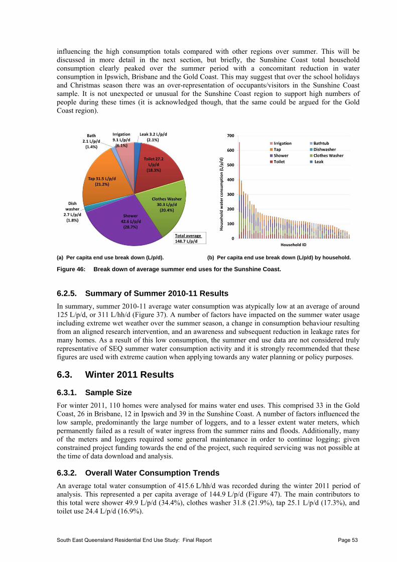
influencing the high consumption totals compared with other regions over summer. This will be discussed in more detail in the next section, but briefly, the Sunshine Coast total household consumption clearly peaked over the summer period with a concomitant reduction in water consumption in Ipswich, Brisbane and the Gold Coast. This may suggest that over the school holidays and Christmas season there was an over-representation of occupants/visitors in the Sunshine Coast sample. It is not unexpected or unusual for the Sunshine Coast region to support high numbers of people during these times (it is acknowledged though, that the same could be argued for the Gold Coast region).
(a) Per capita end use break down (L/p/d). (b) Per capita end use break down (L/p/d) by household.
Figure 46: Break down of average summer end uses for the Sunshine Coast.
6.2.5. Summary of Summer 2010-11 Results
In summary, summer 2010-11 average water consumption was atypically low at an average of around 125 L/p/d, or 311 L/hh/d (Figure 37). A number of factors have impacted on the summer water usage including extreme wet weather over the summer season, a change in consumption behaviour resulting from an aligned research intervention, and an awareness and subsequent reduction in leakage rates for many homes. As a result of this low consumption, the summer end use data are not considered truly representative of SEQ summer water consumption activity and it is strongly recommended that these figures are used with extreme caution when applying towards any water planning or policy purposes.
6.3. Winter 2011 Results
6.3.1. Sample Size
For winter 2011, 110 homes were analysed for mains water end uses. This comprised 33 in the Gold Coast, 26 in Brisbane, 12 in Ipswich and 39 in the Sunshine Coast. A number of factors influenced the low sample, predominantly the large number of loggers, and to a lesser extent water meters, which permanently failed as a result of water ingress from the summer rains and floods. Additionally, many of the meters and loggers required some general maintenance in order to continue logging; given constrained project funding towards the end of the project, such required servicing was not possible at the time of data download and analysis.
6.3.2. Overall Water Consumption Trends
An average total water consumption of 415.6 L/hh/d was recorded during the winter 2011 period of analysis. This represented a per capita average of 144.9 L/p/d (Figure 47). The main contributors to this total were shower 49.9 L/p/d (34.4%), clothes washer 31.8 (21.9%), tap 25.1 L/p/d (17.3%), and toilet use 24.4 L/p/d (16.9%).
South East Queensland Residential End Use Study: Final Report Page 53
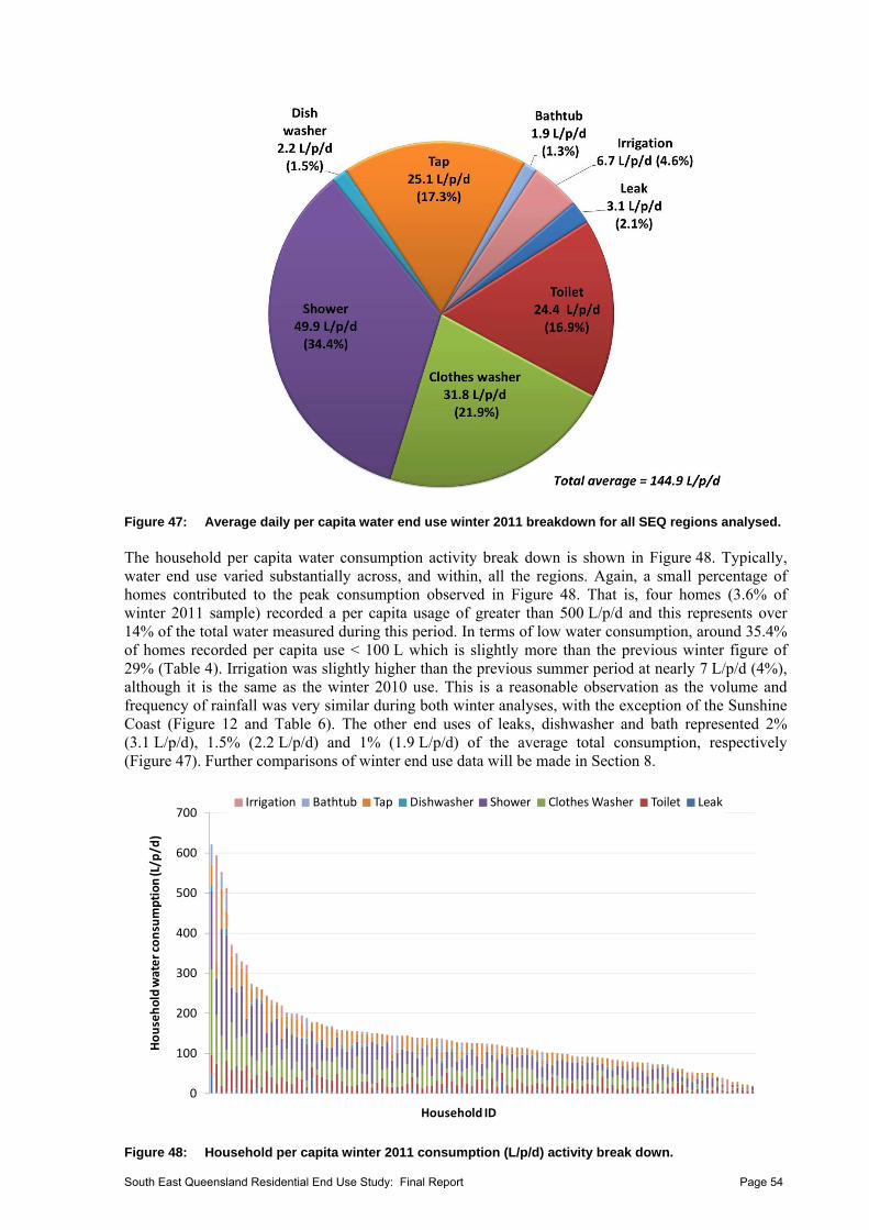
Figure 47: Average daily per capita water end use winter 2011 breakdown for all SEQ regions analysed. The household per capita water consumption activity break down is shown in Figure 48. Typically, water end use varied substantially across, and within, all the regions. Again, a small percentage of homes contributed to the peak consumption observed in Figure 48. That is, four homes (3.6% of winter 2011 sample) recorded a per capita usage of greater than 500 L/p/d and this represents over 14% of the total water measured during this period. In terms of low water consumption, around 35.4% of homes recorded per capita use < 100 L which is slightly more than the previous winter figure of 29% (Table 4). Irrigation was slightly higher than the previous summer period at nearly 7 L/p/d (4%), although it is the same as the winter 2010 use. This is a reasonable observation as the volume and frequency of rainfall was very similar during both winter analyses, with the exception of the Sunshine Coast (Figure 12 and Table 6). The other end uses of leaks, dishwasher and bath represented 2% (3.1 L/p/d), 1.5% (2.2 L/p/d) and 1% (1.9 L/p/d) of the average total consumption, respectively (Figure 47). Further comparisons of winter end use data will be made in Section 8.
0
100
200
300
400
500
600
700
Household water consumption (L/p/d)
Household ID
Irrigation Bathtub Tap Dishwasher Shower Clothes Washer Toilet Leak
Figure 48: Household per capita winter 2011 consumption (L/p/d) activity break down.
South East Queensland Residential End Use Study: Final Report Page 54
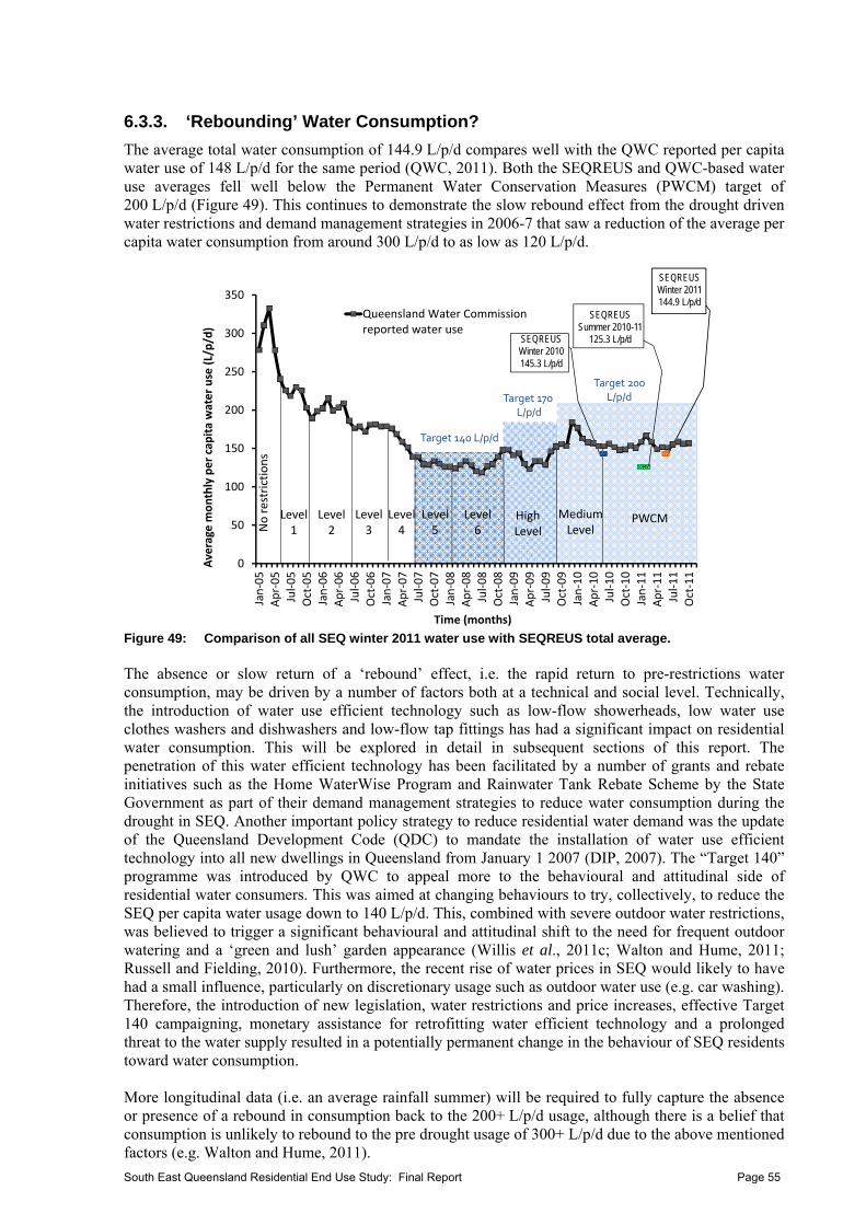
6.3.3. ‘Rebounding’ Water Consumption?
The average total water consumption of 144.9 L/p/d compares well with the QWC reported per capita water use of 148 L/p/d for the same period (QWC, 2011). Both the SEQREUS and QWC-based water use averages fell well below the Permanent Water Conservation Measures (PWCM) target of 200 L/p/d (Figure 49). This continues to demonstrate the slow rebound effect from the drought driven water restrictions and demand management strategies in 2006-7 that saw a reduction of the average per capita water consumption from around 300 L/p/d to as low as 120 L/p/d.
No restrictions
Level1
Level2
Level3
Level4
Level5
Level6
HighLevel
MediumLevel
PWCM
Target 140 L/p/d
Target 170L/p/d
Target 200 L/p/d
SEQREUS Winter 2010145.3 L/p/d
SEQREUS Summer 2010-11
125.3 L/p/d
SEQREUS Winter 2011144.9 L/p/d
0
50
100
150
200
250
300
350
Jan‐05
Apr‐05
Jul‐05
Oct‐05
Jan‐06
Apr‐06
Jul‐06
Oct‐06
Jan‐07
Apr‐07
Jul‐07
Oct‐07
Jan‐08
Apr‐08
Jul‐08
Oct‐08
Jan‐09
Apr‐09
Jul‐09
Oct‐09
Jan‐10
Apr‐10
Jul‐10
Oct‐10
Jan‐11
Apr‐11
Jul‐11
Oct‐11
Average m
onthly per cap
ita water use (L/p/d)
Time (months)
Queensland Water Commissionreported water use
Figure 49: Comparison of all SEQ winter 2011 water use with SEQREUS total average. The absence or slow return of a ‘rebound’ effect, i.e. the rapid return to pre-restrictions water consumption, may be driven by a number of factors both at a technical and social level. Technically, the introduction of water use efficient technology such as low-flow showerheads, low water use clothes washers and dishwashers and low-flow tap fittings has had a significant impact on residential water consumption. This will be explored in detail in subsequent sections of this report. The penetration of this water efficient technology has been facilitated by a number of grants and rebate initiatives such as the Home WaterWise Program and Rainwater Tank Rebate Scheme by the State Government as part of their demand management strategies to reduce water consumption during the drought in SEQ. Another important policy strategy to reduce residential water demand was the update of the Queensland Development Code (QDC) to mandate the installation of water use efficient technology into all new dwellings in Queensland from January 1 2007 (DIP, 2007). The “Target 140” programme was introduced by QWC to appeal more to the behavioural and attitudinal side of residential water consumers. This was aimed at changing behaviours to try, collectively, to reduce the SEQ per capita water usage down to 140 L/p/d. This, combined with severe outdoor water restrictions, was believed to trigger a significant behavioural and attitudinal shift to the need for frequent outdoor watering and a ‘green and lush’ garden appearance (Willis et al., 2011c; Walton and Hume, 2011; Russell and Fielding, 2010). Furthermore, the recent rise of water prices in SEQ would likely to have had a small influence, particularly on discretionary usage such as outdoor water use (e.g. car washing). Therefore, the introduction of new legislation, water restrictions and price increases, effective Target 140 campaigning, monetary assistance for retrofitting water efficient technology and a prolonged threat to the water supply resulted in a potentially permanent change in the behaviour of SEQ residents toward water consumption. More longitudinal data (i.e. an average rainfall summer) will be required to fully capture the absence or presence of a rebound in consumption back to the 200+ L/p/d usage, although there is a belief that consumption is unlikely to rebound to the pre drought usage of 300+ L/p/d due to the above mentioned factors (e.g. Walton and Hume, 2011).
South East Queensland Residential End Use Study: Final Report Page 55
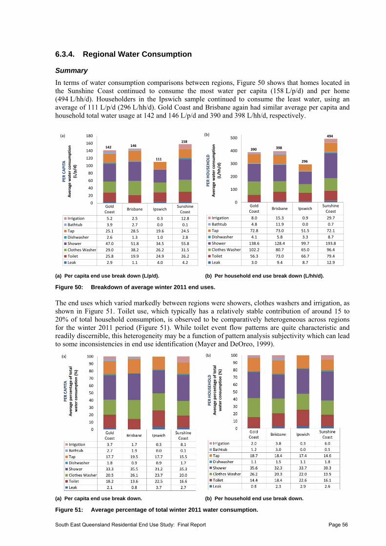
6.3.4. Regional Water Consumption
Summary
In terms of water consumption comparisons between regions, Figure 50 shows that homes located in the Sunshine Coast continued to consume the most water per capita (158 L/p/d) and per home (494 L/hh/d). Householders in the Ipswich sample continued to consume the least water, using an average of 111 L/p/d (296 L/hh/d). Gold Coast and Brisbane again had similar average per capita and household total water usage at 142 and 146 L/p/d and 390 and 398 L/hh/d, respectively.
GoldCoast
Brisbane IpswichSunshineCoast
Irrigation 5.2 2.5 0.3 12.8
Bathtub 3.9 2.7 0.0 0.1
Tap 25.1 28.5 19.6 24.5
Dishwasher 2.6 1.3 1.0 2.8
Shower 47.0 51.8 34.5 55.8
Clothes Washer 29.0 38.2 26.2 31.5
Toilet 25.8 19.9 24.9 26.2
Leak 2.9 1.1 4.0 4.2
0
20
40
60
80
100
120
140
160
180
PER
CAPITA
Average water consumption
(L/p/d)
(a)
142
158
111
146
GoldCoast
Brisbane IpswichSunshineCoast
Irrigation 8.0 15.3 0.9 29.7
Bathtub 4.8 11.9 0.0 0.7
Tap 72.8 73.0 51.5 72.1
Dishwasher 4.1 5.8 3.3 8.7
Shower 138.6 128.4 99.7 193.8
Clothes Washer 102.2 80.7 65.0 96.4
Toilet 56.3 73.0 66.7 79.4
Leak 3.0 9.4 8.7 12.9
0
100
200
300
400
500
PER
HOUSEHOLD
Average water consumption
(L/hh/d)
(b)
390
494
296
398
(a) Per capita end use break down (L/p/d). (b) Per household end use break down (L/hh/d).
Figure 50: Breakdown of average winter 2011 end uses. The end uses which varied markedly between regions were showers, clothes washers and irrigation, as shown in Figure 51. Toilet use, which typically has a relatively stable contribution of around 15 to 20% of total household consumption, is observed to be comparatively heterogeneous across regions for the winter 2011 period (Figure 51). While toilet event flow patterns are quite characteristic and readily discernible, this heterogeneity may be a function of pattern analysis subjectivity which can lead to some inconsistencies in end use identification (Mayer and DeOreo, 1999).
(a) Per capita end use break down. (b) Per household end use break down.
Figure 51: Average percentage of total winter 2011 water consumption.
South East Queensland Residential End Use Study: Final Report Page 56
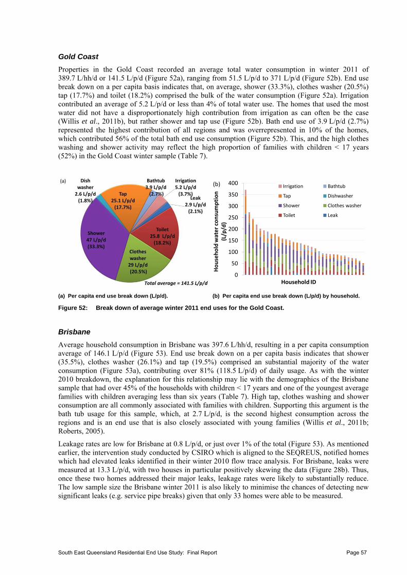
Gold Coast
Properties in the Gold Coast recorded an average total water consumption in winter 2011 of 389.7 L/hh/d or 141.5 L/p/d (Figure 52a), ranging from 51.5 L/p/d to 371 L/p/d (Figure 52b). End use break down on a per capita basis indicates that, on average, shower (33.3%), clothes washer (20.5%) tap (17.7%) and toilet (18.2%) comprised the bulk of the water consumption (Figure 52a). Irrigation contributed an average of 5.2 L/p/d or less than 4% of total water use. The homes that used the most water did not have a disproportionately high contribution from irrigation as can often be the case (Willis et al., 2011b), but rather shower and tap use (Figure 52b). Bath end use of 3.9 L/p/d (2.7%) represented the highest contribution of all regions and was overrepresented in 10% of the homes, which contributed 56% of the total bath end use consumption (Figure 52b). This, and the high clothes washing and shower activity may reflect the high proportion of families with children < 17 years (52%) in the Gold Coast winter sample (Table 7).
0
50
100
150
200
250
300
350
400
Household water consumption
(L/p/d)
Household ID
Irrigation Bathtub
Tap Dishwasher
Shower Clothes washer
Toilet Leak
(b)
(a) Per capita end use break down (L/p/d). (b) Per capita end use break down (L/p/d) by household.
Figure 52: Break down of average winter 2011 end uses for the Gold Coast.
Brisbane
Average household consumption in Brisbane was 397.6 L/hh/d, resulting in a per capita consumption average of 146.1 L/p/d (Figure 53). End use break down on a per capita basis indicates that shower (35.5%), clothes washer (26.1%) and tap (19.5%) comprised an substantial majority of the water consumption (Figure 53a), contributing over 81% (118.5 L/p/d) of daily usage. As with the winter 2010 breakdown, the explanation for this relationship may lie with the demographics of the Brisbane sample that had over 45% of the households with children < 17 years and one of the youngest average families with children averaging less than six years (Table 7). High tap, clothes washing and shower consumption are all commonly associated with families with children. Supporting this argument is the bath tub usage for this sample, which, at 2.7 L/p/d, is the second highest consumption across the regions and is an end use that is also closely associated with young families (Willis et al., 2011b; Roberts, 2005).
Leakage rates are low for Brisbane at 0.8 L/p/d, or just over 1% of the total (Figure 53). As mentioned earlier, the intervention study conducted by CSIRO which is aligned to the SEQREUS, notified homes which had elevated leaks identified in their winter 2010 flow trace analysis. For Brisbane, leaks were measured at 13.3 L/p/d, with two houses in particular positively skewing the data (Figure 28b). Thus, once these two homes addressed their major leaks, leakage rates were likely to substantially reduce. The low sample size the Brisbane winter 2011 is also likely to minimise the chances of detecting new significant leaks (e.g. service pipe breaks) given that only 33 homes were able to be measured.
South East Queensland Residential End Use Study: Final Report Page 57
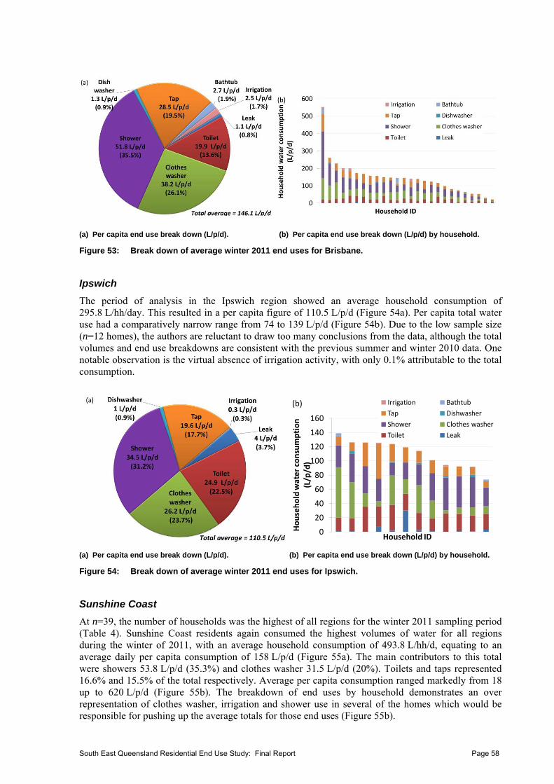
(a) Per capita end use break down (L/p/d). (b) Per capita end use break down (L/p/d) by household.
Figure 53: Break down of average winter 2011 end uses for Brisbane.
Ipswich
The period of analysis in the Ipswich region showed an average household consumption of 295.8 L/hh/day. This resulted in a per capita figure of 110.5 L/p/d (Figure 54a). Per capita total water use had a comparatively narrow range from 74 to 139 L/p/d (Figure 54b). Due to the low sample size (n=12 homes), the authors are reluctant to draw too many conclusions from the data, although the total volumes and end use breakdowns are consistent with the previous summer and winter 2010 data. One notable observation is the virtual absence of irrigation activity, with only 0.1% attributable to the total consumption.
0
20
40
60
80
100
120
140
160
Household water consumption
(L/p/d)
Household ID
Irrigation Bathtub
Tap Dishwasher
Shower Clothes washer
Toilet Leak
(b)
(a) Per capita end use break down (L/p/d). (b) Per capita end use break down (L/p/d) by household.
Figure 54: Break down of average winter 2011 end uses for Ipswich.
Sunshine Coast
At n=39, the number of households was the highest of all regions for the winter 2011 sampling period (Table 4). Sunshine Coast residents again consumed the highest volumes of water for all regions during the winter of 2011, with an average household consumption of 493.8 L/hh/d, equating to an average daily per capita consumption of 158 L/p/d (Figure 55a). The main contributors to this total were showers 53.8 L/p/d (35.3%) and clothes washer 31.5 L/p/d (20%). Toilets and taps represented 16.6% and 15.5% of the total respectively. Average per capita consumption ranged markedly from 18 up to 620 L/p/d (Figure 55b). The breakdown of end uses by household demonstrates an over representation of clothes washer, irrigation and shower use in several of the homes which would be responsible for pushing up the average totals for those end uses (Figure 55b).
South East Queensland Residential End Use Study: Final Report Page 58
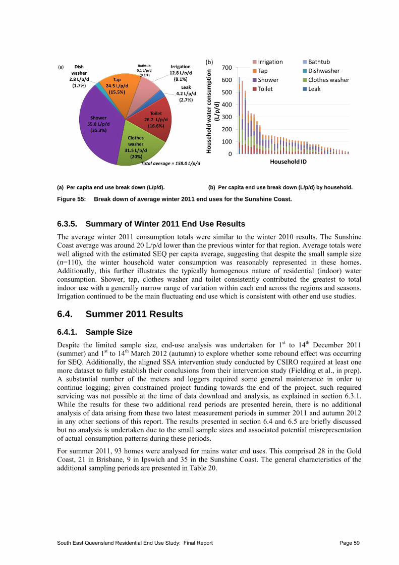
0
100
200
300
400
500
600
700
Household water consumption
(L/p/d)
Household ID
Irrigation Bathtub
Tap Dishwasher
Shower Clothes washer
Toilet Leak
(b)
(a) Per capita end use break down (L/p/d). (b) Per capita end use break down (L/p/d) by household.
Figure 55: Break down of average winter 2011 end uses for the Sunshine Coast.
6.3.5. Summary of Winter 2011 End Use Results
The average winter 2011 consumption totals were similar to the winter 2010 results. The Sunshine Coast average was around 20 L/p/d lower than the previous winter for that region. Average totals were well aligned with the estimated SEQ per capita average, suggesting that despite the small sample size (n=110), the winter household water consumption was reasonably represented in these homes. Additionally, this further illustrates the typically homogenous nature of residential (indoor) water consumption. Shower, tap, clothes washer and toilet consistently contributed the greatest to total indoor use with a generally narrow range of variation within each end across the regions and seasons. Irrigation continued to be the main fluctuating end use which is consistent with other end use studies.
6.4. Summer 2011 Results
6.4.1. Sample Size
Despite the limited sample size, end-use analysis was undertaken for 1st to 14th December 2011 (summer) and 1st to 14th March 2012 (autumn) to explore whether some rebound effect was occurring for SEQ. Additionally, the aligned SSA intervention study conducted by CSIRO required at least one more dataset to fully establish their conclusions from their intervention study (Fielding et al., in prep). A substantial number of the meters and loggers required some general maintenance in order to continue logging; given constrained project funding towards the end of the project, such required servicing was not possible at the time of data download and analysis, as explained in section 6.3.1. While the results for these two additional read periods are presented herein, there is no additional analysis of data arising from these two latest measurement periods in summer 2011 and autumn 2012 in any other sections of this report. The results presented in section 6.4 and 6.5 are briefly discussed but no analysis is undertaken due to the small sample sizes and associated potential misrepresentation of actual consumption patterns during these periods.
For summer 2011, 93 homes were analysed for mains water end uses. This comprised 28 in the Gold Coast, 21 in Brisbane, 9 in Ipswich and 35 in the Sunshine Coast. The general characteristics of the additional sampling periods are presented in Table 20.
South East Queensland Residential End Use Study: Final Report Page 59
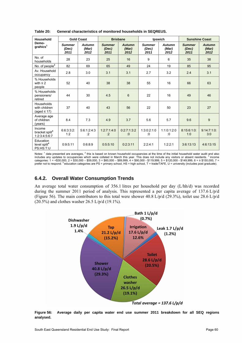
Table 20: General characteristics of monitored households in SEQREUS.
Gold Coast Brisbane Ipswich Sunshine Coast Household Demo-grahics1 Summer
(Dec) 2011
Autumn (Mar) 2012
Summer (Dec) 2011
Autumn (Mar) 2012
Summer (Dec) 2011
Autumn (Mar) 2012
Summer (Dec) 2011
Autumn (Mar) 2012
No. of households
28 23 25 16 9 6 35 38
No. of people2 82 69 65 49 24 19 85 95
Av. Household occupancy
2.8 3.0 3.1 3.1 2.7 3.2 2.4 3.1
% Households with ≤ 2 people
52 40 38 38 55 16 66 63
% Households pensioners/ retired
44 30 4.5 6 22 16 49 46
Households with children (aged ≤ 17)
37 40 43 56 22 50 23 27
Average age of children (years)
8.4 7.3 4.9 3.7 5.6 5.7 9.6 9
Income bracket split3
1:2:3:4:5:6:7
6:6:3:3:2:1:2
5:6:1:2:4:3:2
1:2:7:1:4:0:2
0:2:7:1:3:2:0
1:3:0:2:1:0:0
1:1:0:1:2:0:0
8:15:6:1:0:1:0
9:14:7:1:0:3:0
Education level split4
PS:HS:T:U 0:9:5:11 0:6:8:9 0:5:5:10 0:2:3:11 2:2:4:1 1:2:2:1 3:6:13:13 4:6:13:15
Notes: 1 data presented are averages, 2 this is based on known household occupancies at the time of the initial household water audit and also includes any updates to occupancies which were collated in March this year. This does not include any visitors or absent residents. 3 income categories: 1 = <$30,000, 2 = $30,000 – $59,000, 3 = $60,000 – $89,999, 4 = $90,000 - $119,999, 5 = $120,000 - $149,999, 6 = ≥ $150,000, 7 = prefer not to respond. 4 education categories are PS = primary school, HS = high school, T = trade/TAFE, U = university (includes post graduate).
6.4.2. Overall Water Consumption Trends
An average total water consumption of 356.1 litres per household per day (L/hh/d) was recorded during the summer 2011 period of analysis. This represented a per capita average of 137.6 L/p/d (Figure 56). The main contributors to this total were shower 40.8 L/p/d (29.3%), toilet use 28.6 L/p/d (20.5%) and clothes washer 26.5 L/p/d (19.1%).
Figure 56: Average daily per capita water end use summer 2011 breakdown for all SEQ regions analysed.
South East Queensland Residential End Use Study: Final Report Page 60
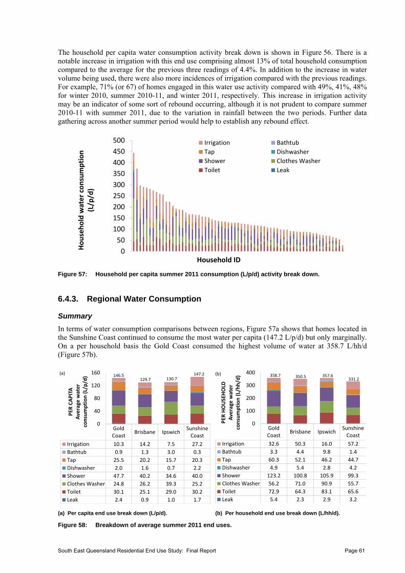
The household per capita water consumption activity break down is shown in Figure 56. There is a notable increase in irrigation with this end use comprising almost 13% of total household consumption compared to the average for the previous three readings of 4.4%. In addition to the increase in water volume being used, there were also more incidences of irrigation compared with the previous readings. For example, 71% (or 67) of homes engaged in this water use activity compared with 49%, 41%, 48% for winter 2010, summer 2010-11, and winter 2011, respectively. This increase in irrigation activity may be an indicator of some sort of rebound occurring, although it is not prudent to compare summer 2010-11 with summer 2011, due to the variation in rainfall between the two periods. Further data gathering across another summer period would help to establish any rebound effect.
0
50
100
150
200
250
300
350
400
450
500
Household water consumption
(L/p/d)
Household ID
Irrigation Bathtub
Tap Dishwasher
Shower Clothes Washer
Toilet Leak
Figure 57: Household per capita summer 2011 consumption (L/p/d) activity break down.
6.4.3. Regional Water Consumption
Summary
In terms of water consumption comparisons between regions, Figure 57a shows that homes located in the Sunshine Coast continued to consume the most water per capita (147.2 L/p/d) but only marginally. On a per household basis the Gold Coast consumed the highest volume of water at 358.7 L/hh/d (Figure 57b).
GoldCoast
Brisbane IpswichSunshineCoast
Irrigation 10.3 14.2 7.5 27.2
Bathtub 0.9 1.3 3.0 0.3
Tap 25.5 20.2 15.7 20.3
Dishwasher 2.0 1.6 0.7 2.2
Shower 47.7 40.2 34.6 40.0
Clothes Washer 24.8 26.2 39.3 25.2
Toilet 30.1 25.1 29.0 30.2
Leak 2.4 0.9 1.0 1.7
0
40
80
120
160
PER
CAPITA
Average water
consumption (L/p/d) 146.5 147.2
130.7129.7
(a)
GoldCoast
Brisbane IpswichSunshineCoast
Irrigation 32.6 50.3 16.0 57.2
Bathtub 3.3 4.4 9.8 1.4
Tap 60.3 52.1 46.2 44.7
Dishwasher 4.9 5.4 2.8 4.2
Shower 123.2 100.8 105.9 99.3
Clothes Washer 56.2 71.0 90.9 55.7
Toilet 72.9 64.3 83.1 65.6
Leak 5.4 2.3 2.9 3.2
0
100
200
300
400
PER
HOUSEHOLD
Average water
consumption (L/hh/d) 358.7
331.2357.6350.5
(b)
(a) Per capita end use break down (L/p/d). (b) Per household end use break down (L/hh/d).
Figure 58: Breakdown of average summer 2011 end uses.
South East Queensland Residential End Use Study: Final Report Page 61
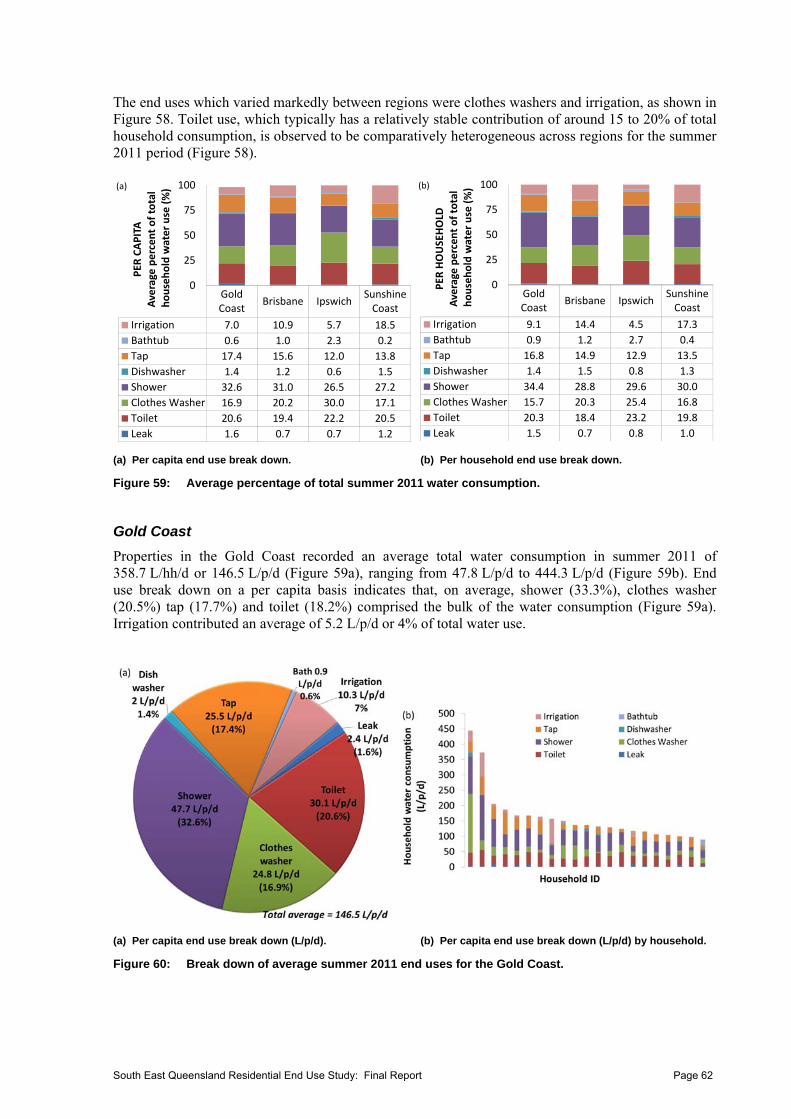
The end uses which varied markedly between regions were clothes washers and irrigation, as shown in Figure 58. Toilet use, which typically has a relatively stable contribution of around 15 to 20% of total household consumption, is observed to be comparatively heterogeneous across regions for the summer 2011 period (Figure 58).
GoldCoast
Brisbane IpswichSunshineCoast
Irrigation 7.0 10.9 5.7 18.5
Bathtub 0.6 1.0 2.3 0.2
Tap 17.4 15.6 12.0 13.8
Dishwasher 1.4 1.2 0.6 1.5
Shower 32.6 31.0 26.5 27.2
Clothes Washer 16.9 20.2 30.0 17.1
Toilet 20.6 19.4 22.2 20.5
Leak 1.6 0.7 0.7 1.2
0
25
50
75
100
PER
CAPITA
Average percent of total
household water use (%) (a)
GoldCoast
Brisbane IpswichSunshineCoast
Irrigation 9.1 14.4 4.5 17.3
Bathtub 0.9 1.2 2.7 0.4
Tap 16.8 14.9 12.9 13.5
Dishwasher 1.4 1.5 0.8 1.3
Shower 34.4 28.8 29.6 30.0
Clothes Washer 15.7 20.3 25.4 16.8
Toilet 20.3 18.4 23.2 19.8
Leak 1.5 0.7 0.8 1.0
0
25
50
75
100
PER
HOUSEHOLD
Average percen
t of total
household water use (%) (b)
(a) Per capita end use break down. (b) Per household end use break down.
Figure 59: Average percentage of total summer 2011 water consumption.
Gold Coast
Properties in the Gold Coast recorded an average total water consumption in summer 2011 of 358.7 L/hh/d or 146.5 L/p/d (Figure 59a), ranging from 47.8 L/p/d to 444.3 L/p/d (Figure 59b). End use break down on a per capita basis indicates that, on average, shower (33.3%), clothes washer (20.5%) tap (17.7%) and toilet (18.2%) comprised the bulk of the water consumption (Figure 59a). Irrigation contributed an average of 5.2 L/p/d or 4% of total water use.
(a) Per capita end use break down (L/p/d). (b) Per capita end use break down (L/p/d) by household.
Figure 60: Break down of average summer 2011 end uses for the Gold Coast.
South East Queensland Residential End Use Study: Final Report Page 62
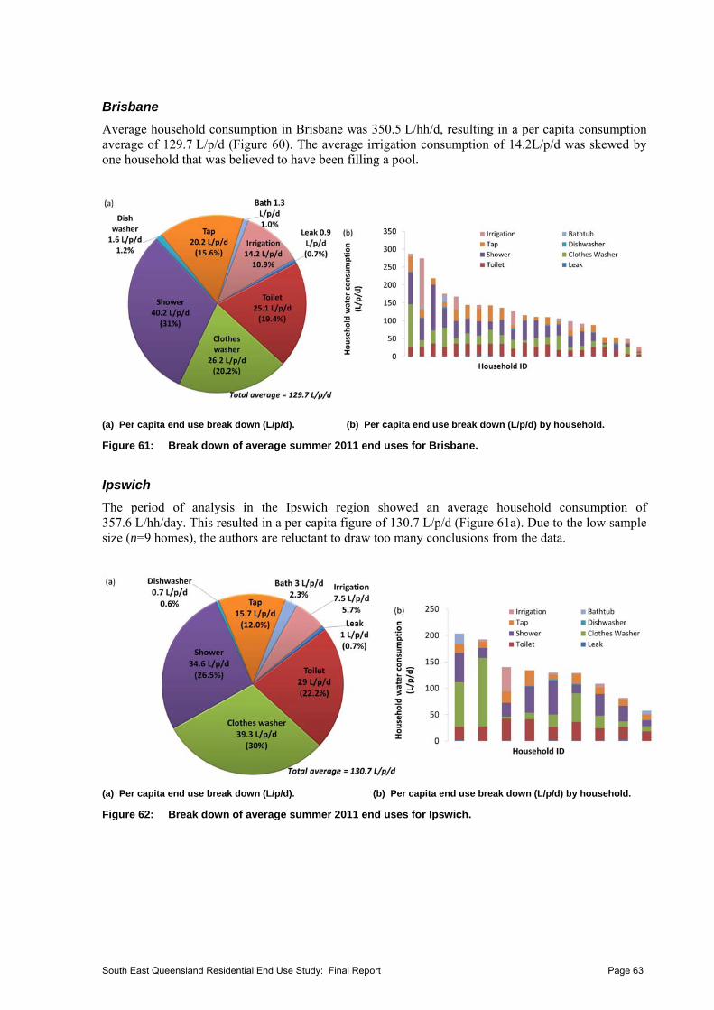
Brisbane
Average household consumption in Brisbane was 350.5 L/hh/d, resulting in a per capita consumption average of 129.7 L/p/d (Figure 60). The average irrigation consumption of 14.2L/p/d was skewed by one household that was believed to have been filling a pool.
(a) Per capita end use break down (L/p/d). (b) Per capita end use break down (L/p/d) by household.
Figure 61: Break down of average summer 2011 end uses for Brisbane.
Ipswich
The period of analysis in the Ipswich region showed an average household consumption of 357.6 L/hh/day. This resulted in a per capita figure of 130.7 L/p/d (Figure 61a). Due to the low sample size (n=9 homes), the authors are reluctant to draw too many conclusions from the data.
(a) Per capita end use break down (L/p/d). (b) Per capita end use break down (L/p/d) by household.
Figure 62: Break down of average summer 2011 end uses for Ipswich.
South East Queensland Residential End Use Study: Final Report Page 63
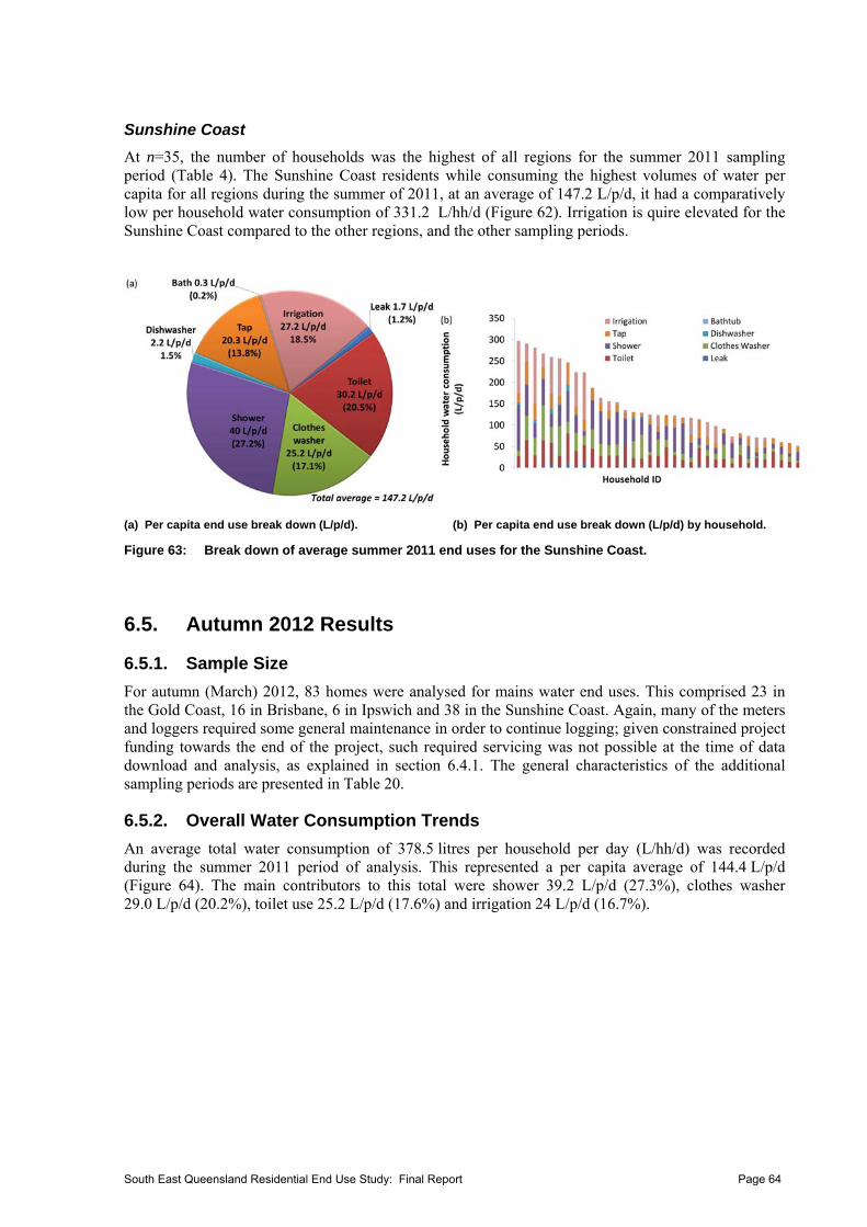
Sunshine Coast
At n=35, the number of households was the highest of all regions for the summer 2011 sampling period (Table 4). The Sunshine Coast residents while consuming the highest volumes of water per capita for all regions during the summer of 2011, at an average of 147.2 L/p/d, it had a comparatively low per household water consumption of 331.2 L/hh/d (Figure 62). Irrigation is quire elevated for the Sunshine Coast compared to the other regions, and the other sampling periods.
(a) Per capita end use break down (L/p/d). (b) Per capita end use break down (L/p/d) by household.
Figure 63: Break down of average summer 2011 end uses for the Sunshine Coast.
6.5. Autumn 2012 Results
6.5.1. Sample Size
For autumn (March) 2012, 83 homes were analysed for mains water end uses. This comprised 23 in the Gold Coast, 16 in Brisbane, 6 in Ipswich and 38 in the Sunshine Coast. Again, many of the meters and loggers required some general maintenance in order to continue logging; given constrained project funding towards the end of the project, such required servicing was not possible at the time of data download and analysis, as explained in section 6.4.1. The general characteristics of the additional sampling periods are presented in Table 20.
6.5.2. Overall Water Consumption Trends
An average total water consumption of 378.5 litres per household per day (L/hh/d) was recorded during the summer 2011 period of analysis. This represented a per capita average of 144.4 L/p/d (Figure 64). The main contributors to this total were shower 39.2 L/p/d (27.3%), clothes washer 29.0 L/p/d (20.2%), toilet use 25.2 L/p/d (17.6%) and irrigation 24 L/p/d (16.7%).
South East Queensland Residential End Use Study: Final Report Page 64
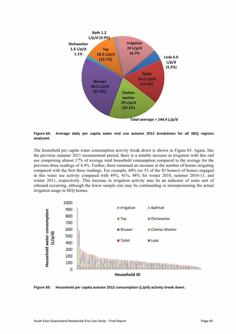
Figure 64: Average daily per capita water end use autumn 2012 breakdown for all SEQ regions analysed.
The household per capita water consumption activity break down is shown in Figure 65. Again, like the previous summer 2011 measurement period, there is a notable increase in irrigation with this end use comprising almost 17% of average total household consumption compared to the average for the previous three readings of 4.4%. Further, there remained an increase in the number of homes irrigating compared with the first three readings. For example, 60% (or 55 of the 83 homes) of homes engaged in this water use activity compared with 49%, 41%, 48% for winter 2010, summer 2010-11, and winter 2011, respectively. This increase in irrigation activity may be an indicator of some sort of rebound occurring, although the lower sample size may be confounding or misrepresenting the actual irrigation usage in SEQ homes.
Figure 65: Household per capita autumn 2012 consumption (L/p/d) activity break down.
South East Queensland Residential End Use Study: Final Report Page 65
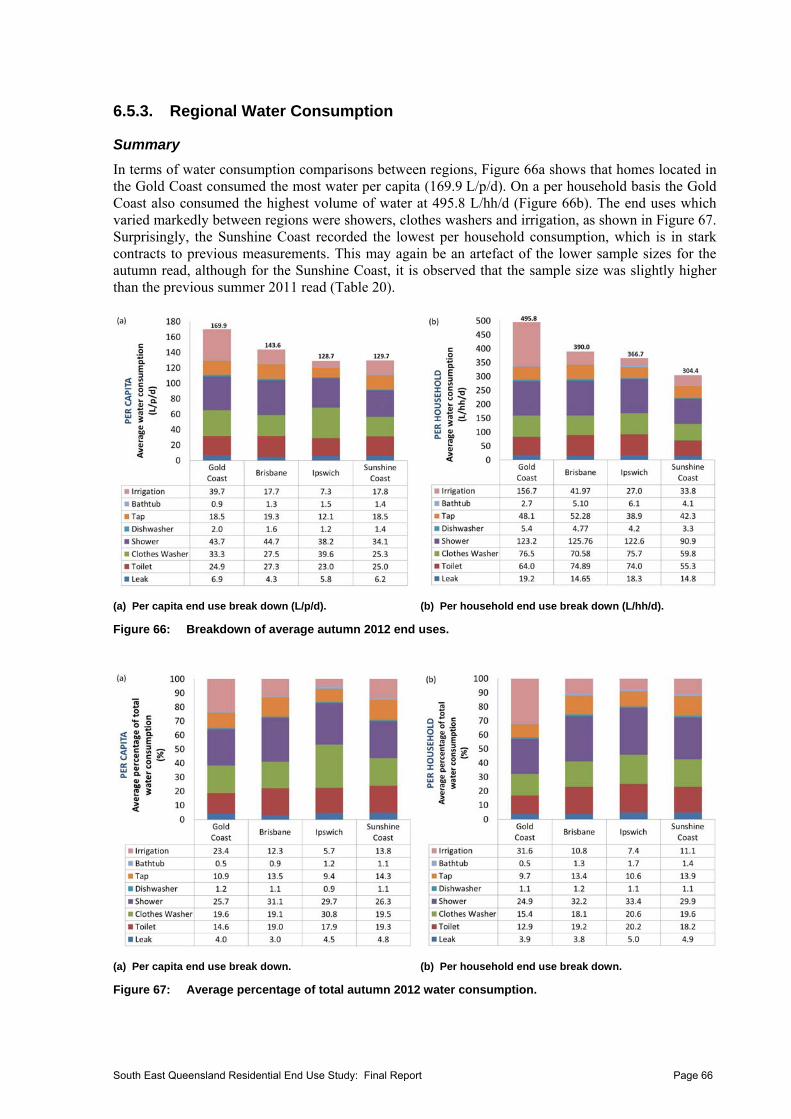
6.5.3. Regional Water Consumption
Summary
In terms of water consumption comparisons between regions, Figure 66a shows that homes located in the Gold Coast consumed the most water per capita (169.9 L/p/d). On a per household basis the Gold Coast also consumed the highest volume of water at 495.8 L/hh/d (Figure 66b). The end uses which varied markedly between regions were showers, clothes washers and irrigation, as shown in Figure 67. Surprisingly, the Sunshine Coast recorded the lowest per household consumption, which is in stark contracts to previous measurements. This may again be an artefact of the lower sample sizes for the autumn read, although for the Sunshine Coast, it is observed that the sample size was slightly higher than the previous summer 2011 read (Table 20).
(a) Per capita end use break down (L/p/d). (b) Per household end use break down (L/hh/d).
Figure 66: Breakdown of average autumn 2012 end uses.
(a) Per capita end use break down. (b) Per household end use break down.
Figure 67: Average percentage of total autumn 2012 water consumption.
South East Queensland Residential End Use Study: Final Report Page 66
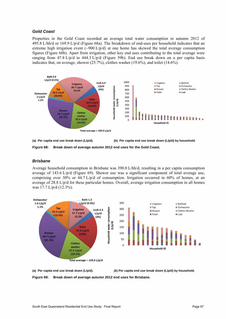
Gold Coast
Properties in the Gold Coast recorded an average total water consumption in autumn 2012 of 495.8 L/hh/d or 169.9 L/p/d (Figure 68a). The breakdown of end-uses per household indicates that an extreme high irrigation event (~900 L/p/d) at one home has skewed the total average consumption figures (Figure 68b). Apart from irrigation, other key end uses contributing to the total average were ranging from 47.8 L/p/d to 444.3 L/p/d (Figure 59b). End use break down on a per capita basis indicates that, on average, shower (25.7%), clothes washer (19.6%), and toilet (14.6%).
(a) Per capita end use break down (L/p/d). (b) Per capita end use break down (L/p/d) by household.
Figure 68: Break down of average autumn 2012 end uses for the Gold Coast.
Brisbane
Average household consumption in Brisbane was 390.0 L/hh/d, resulting in a per capita consumption average of 143.6 L/p/d (Figure 69). Shower use was a significant component of total average use, comprising over 30% or 44.7 L/p/d of consumption. Irrigation occurred in 60% of homes, at an average of 28.8 L/p/d for these particular homes. Overall, average irrigation consumption in all homes was 17.7 L/p/d (12.3%).
(a) Per capita end use break down (L/p/d). (b) Per capita end use break down (L/p/d) by household.
Figure 69: Break down of average autumn 2012 end uses for Brisbane.
South East Queensland Residential End Use Study: Final Report Page 67
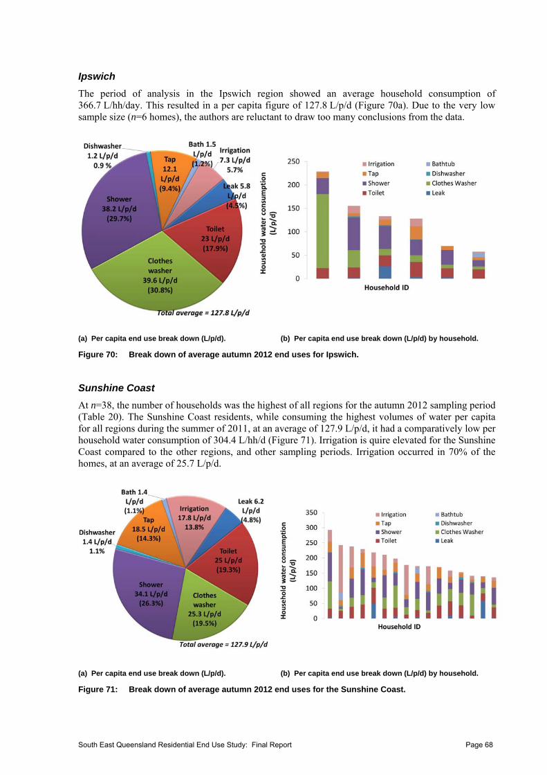
Ipswich
The period of analysis in the Ipswich region showed an average household consumption of 366.7 L/hh/day. This resulted in a per capita figure of 127.8 L/p/d (Figure 70a). Due to the very low sample size (n=6 homes), the authors are reluctant to draw too many conclusions from the data.
(a) Per capita end use break down (L/p/d). (b) Per capita end use break down (L/p/d) by household.
Figure 70: Break down of average autumn 2012 end uses for Ipswich.
Sunshine Coast
At n=38, the number of households was the highest of all regions for the autumn 2012 sampling period (Table 20). The Sunshine Coast residents, while consuming the highest volumes of water per capita for all regions during the summer of 2011, at an average of 127.9 L/p/d, it had a comparatively low per household water consumption of 304.4 L/hh/d (Figure 71). Irrigation is quire elevated for the Sunshine Coast compared to the other regions, and other sampling periods. Irrigation occurred in 70% of the homes, at an average of 25.7 L/p/d.
(a) Per capita end use break down (L/p/d). (b) Per capita end use break down (L/p/d) by household.
Figure 71: Break down of average autumn 2012 end uses for the Sunshine Coast.
South East Queensland Residential End Use Study: Final Report Page 68
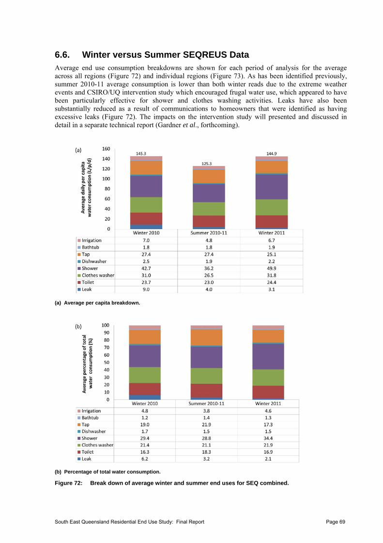
6.6. Winter versus Summer SEQREUS Data Average end use consumption breakdowns are shown for each period of analysis for the average across all regions (Figure 72) and individual regions (Figure 73). As has been identified previously, summer 2010-11 average consumption is lower than both winter reads due to the extreme weather events and CSIRO/UQ intervention study which encouraged frugal water use, which appeared to have been particularly effective for shower and clothes washing activities. Leaks have also been substantially reduced as a result of communications to homeowners that were identified as having excessive leaks (Figure 72). The impacts on the intervention study will presented and discussed in detail in a separate technical report (Gardner et al., forthcoming).
(a) Average per capita breakdown.
(b) Percentage of total water consumption.
Figure 72: Break down of average winter and summer end uses for SEQ combined.
South East Queensland Residential End Use Study: Final Report Page 69
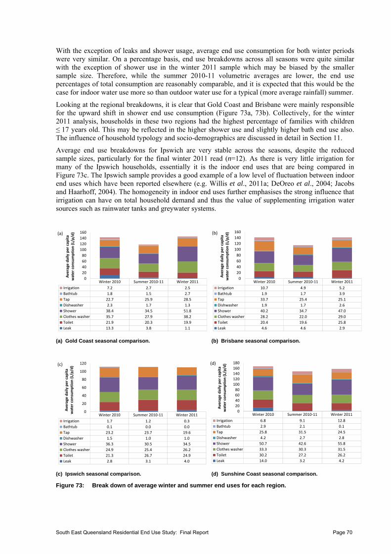
With the exception of leaks and shower usage, average end use consumption for both winter periods were very similar. On a percentage basis, end use breakdowns across all seasons were quite similar with the exception of shower use in the winter 2011 sample which may be biased by the smaller sample size. Therefore, while the summer 2010-11 volumetric averages are lower, the end use percentages of total consumption are reasonably comparable, and it is expected that this would be the case for indoor water use more so than outdoor water use for a typical (more average rainfall) summer.
Looking at the regional breakdowns, it is clear that Gold Coast and Brisbane were mainly responsible for the upward shift in shower end use consumption (Figure 73a, 73b). Collectively, for the winter 2011 analysis, households in these two regions had the highest percentage of families with children ≤ 17 years old. This may be reflected in the higher shower use and slightly higher bath end use also. The influence of household typology and socio-demographics are discussed in detail in Section 11.
Average end use breakdowns for Ipswich are very stable across the seasons, despite the reduced sample sizes, particularly for the final winter 2011 read (n=12). As there is very little irrigation for many of the Ipswich households, essentially it is the indoor end uses that are being compared in Figure 73c. The Ipswich sample provides a good example of a low level of fluctuation between indoor end uses which have been reported elsewhere (e.g. Willis et al., 2011a; DeOreo et al., 2004; Jacobs and Haarhoff, 2004). The homogeneity in indoor end uses further emphasises the strong influence that irrigation can have on total household demand and thus the value of supplementing irrigation water sources such as rainwater tanks and greywater systems.
Winter 2010 Summer 2010‐11 Winter 2011
Irrigation 7.2 2.7 2.5
Bathtub 1.8 1.5 2.7
Tap 22.7 25.9 28.5
Dishwasher 2.3 1.7 1.3
Shower 38.4 34.5 51.8
Clothes washer 35.7 27.9 38.2
Toilet 21.9 20.3 19.9
Leak 13.3 3.8 1.1
0
20
40
60
80
100
120
140
160
Average daily per cap
ita
water consumption (L/p/d)(a)
Winter 2010 Summer 2010‐11 Winter 2011
Irrigation 10.7 4.9 5.2
Bathtub 1.9 1.7 3.9
Tap 33.7 25.4 25.1
Dishwasher 1.9 1.7 2.6
Shower 40.2 34.7 47.0
Clothes washer 28.2 22.0 29.0
Toilet 20.4 19.6 25.8
Leak 4.6 4.6 2.9
0
20
40
60
80
100
120
140
160
Average daily per capita
water consumption (L/p/d)(b)
(a) Gold Coast seasonal comparison. (b) Brisbane seasonal comparison.
Winter 2010 Summer 2010‐11 Winter 2011
Irrigation 1.7 1.2 0.3
Bathtub 0.1 0.0 0.0
Tap 23.2 23.7 19.6
Dishwasher 1.5 1.0 1.0
Shower 36.3 30.5 34.5
Clothes washer 24.9 25.4 26.2
Toilet 21.3 26.7 24.9
Leak 2.8 3.1 4.0
0
20
40
60
80
100
120
Average daily per capita
water consumption (L/p/d)(c)
Winter 2010 Summer 2010‐11 Winter 2011
Irrigation 6.8 9.1 12.8
Bathtub 2.9 2.1 0.1
Tap 25.8 31.5 24.5
Dishwasher 4.2 2.7 2.8
Shower 50.7 42.6 55.8
Clothes washer 33.3 30.3 31.5
Toilet 30.2 27.2 26.2
Leak 14.0 3.2 4.2
0
20
40
6080
100
120
140
160
180
Average daily per capita
water consumption (L/p/d)(d)
(c) Ipswich seasonal comparison. (d) Sunshine Coast seasonal comparison.
Figure 73: Break down of average winter and summer end uses for each region.
South East Queensland Residential End Use Study: Final Report Page 70
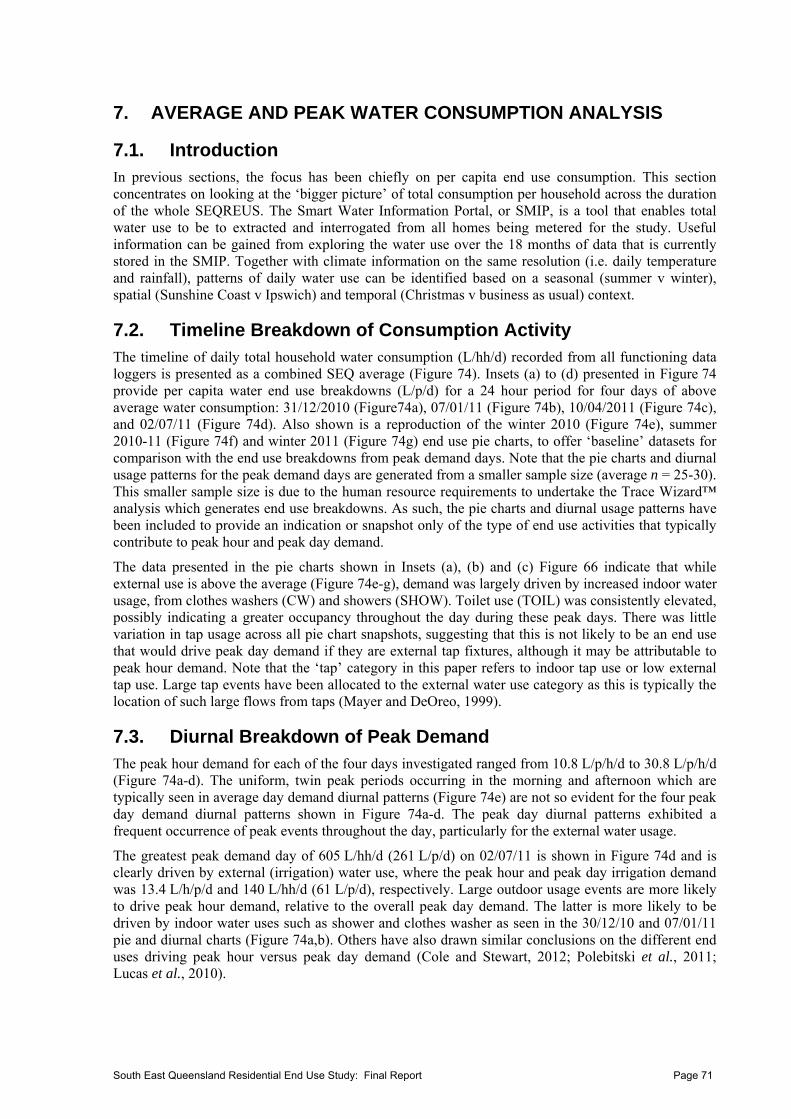
7. AVERAGE AND PEAK WATER CONSUMPTION ANALYSIS
7.1. Introduction In previous sections, the focus has been chiefly on per capita end use consumption. This section concentrates on looking at the ‘bigger picture’ of total consumption per household across the duration of the whole SEQREUS. The Smart Water Information Portal, or SMIP, is a tool that enables total water use to be to extracted and interrogated from all homes being metered for the study. Useful information can be gained from exploring the water use over the 18 months of data that is currently stored in the SMIP. Together with climate information on the same resolution (i.e. daily temperature and rainfall), patterns of daily water use can be identified based on a seasonal (summer v winter), spatial (Sunshine Coast v Ipswich) and temporal (Christmas v business as usual) context.
7.2. Timeline Breakdown of Consumption Activity The timeline of daily total household water consumption (L/hh/d) recorded from all functioning data loggers is presented as a combined SEQ average (Figure 74). Insets (a) to (d) presented in Figure 74 provide per capita water end use breakdowns (L/p/d) for a 24 hour period for four days of above average water consumption: 31/12/2010 (Figure74a), 07/01/11 (Figure 74b), 10/04/2011 (Figure 74c), and 02/07/11 (Figure 74d). Also shown is a reproduction of the winter 2010 (Figure 74e), summer 2010-11 (Figure 74f) and winter 2011 (Figure 74g) end use pie charts, to offer ‘baseline’ datasets for comparison with the end use breakdowns from peak demand days. Note that the pie charts and diurnal usage patterns for the peak demand days are generated from a smaller sample size (average n = 25-30). This smaller sample size is due to the human resource requirements to undertake the Trace Wizard™ analysis which generates end use breakdowns. As such, the pie charts and diurnal usage patterns have been included to provide an indication or snapshot only of the type of end use activities that typically contribute to peak hour and peak day demand.
The data presented in the pie charts shown in Insets (a), (b) and (c) Figure 66 indicate that while external use is above the average (Figure 74e-g), demand was largely driven by increased indoor water usage, from clothes washers (CW) and showers (SHOW). Toilet use (TOIL) was consistently elevated, possibly indicating a greater occupancy throughout the day during these peak days. There was little variation in tap usage across all pie chart snapshots, suggesting that this is not likely to be an end use that would drive peak day demand if they are external tap fixtures, although it may be attributable to peak hour demand. Note that the ‘tap’ category in this paper refers to indoor tap use or low external tap use. Large tap events have been allocated to the external water use category as this is typically the location of such large flows from taps (Mayer and DeOreo, 1999).
7.3. Diurnal Breakdown of Peak Demand The peak hour demand for each of the four days investigated ranged from 10.8 L/p/h/d to 30.8 L/p/h/d (Figure 74a-d). The uniform, twin peak periods occurring in the morning and afternoon which are typically seen in average day demand diurnal patterns (Figure 74e) are not so evident for the four peak day demand diurnal patterns shown in Figure 74a-d. The peak day diurnal patterns exhibited a frequent occurrence of peak events throughout the day, particularly for the external water usage.
The greatest peak demand day of 605 L/hh/d (261 L/p/d) on 02/07/11 is shown in Figure 74d and is clearly driven by external (irrigation) water use, where the peak hour and peak day irrigation demand was 13.4 L/h/p/d and 140 L/hh/d (61 L/p/d), respectively. Large outdoor usage events are more likely to drive peak hour demand, relative to the overall peak day demand. The latter is more likely to be driven by indoor water uses such as shower and clothes washer as seen in the 30/12/10 and 07/01/11 pie and diurnal charts (Figure 74a,b). Others have also drawn similar conclusions on the different end uses driving peak hour versus peak day demand (Cole and Stewart, 2012; Polebitski et al., 2011; Lucas et al., 2010).
South East Queensland Residential End Use Study: Final Report Page 71
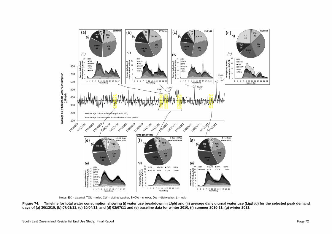
100
200
300
400
500
600
700
800
Average daily household water consumption
(L/hh/d)
Time (months)
Average daily total consumption in SEQ
Average consumption across the measured period
PD/AD 1.5PD/AD
1.2
PD/AD1.7
(a) 30/12/10 10/04/11 02/07/11(c) (d)(i)
(ii)
(i)
(ii)
(i)
(ii)
PD/AD1.3
07/01/11(b)
(i)
(ii)
(e)(i)
(ii)
14 – 28 June Winter, 2010
TOIL 34
CW42
SHOW58
TAP 27
EX13
0
4
8
12
16
1 3 5 7 9 11 13 15 17 19 21 23
Average daily diurnal
consumption (L/p/h/d)
Hour of day
EX
BATH
TAP
SHOW
CW
TOIL
0
5
10
15
20
25
1 3 5 7 9 11 13 15 17 19 21 23
Average daily diurnal
consumption (L/p/h/d)
Hour of day
EX
BATH
TAP
SHOW
CW
TOIL
0
4
8
12
16
20
1 3 5 7 9 11 13 15 17 19 21 23Average daily diurnal
consumption (L/p/h/d)
Hour of day
EXTAPSHOWCWTOILLEAK
TOIL 34
CW57
SHOW41
TAP 23
EX12
TOIL 24
CW31SHOW
43
TAP 28
0
2
4
6
8
10
12
14
1 3 5 7 9 11 13 15 17 19 21 23
Average daily diurnal
consumption (L/p/h/d)
Hour of day
EX
BATH
TAP
DW
SHOW
CW
TOIL
LEAK
TOIL37
CW56
SHOW61
TAP24
(f)(i)
1 Dec – 22 FebSummer 2010‐11 (g)
(i)
(ii)
1– 14 June Winter 2011
0
10
20
30
40
1 3 5 7 9 11 13 15 17 19 21 23
Average daily diurnal
consumption (L/p/h/d)
Hour of day
EX
BATH
TAP
SHOW
CW
TOIL
0
2
4
6
8
10
12
14
1 3 5 7 9 11 13 15 17 19 21 23Average daily diurnal
consumption (L/p/h/d)
Hour of day
EX BATH TAP DW
SHOW CW TOIL Leak
0
2
4
6
8
10
12
14
1 3 5 7 9 11 13 15 17 19 21 23
Averagedaily diurnal
consumption (L/p/h/d)
Hour of day
EX BATH TAP DW
SHOW CW TOIL Leak
(ii)
TOIL24
CW32
SHOW50
TAP25
L 4
TOIL23
CW27
SHOW 36
TAP 27
EX 5
TOIL31
CW80
SHOW52
TAP30
EX62
Notes: EX = external, TOIL = toilet, CW = clothes washer, SHOW = shower, DW = dishwasher, L = leak.
Figure 74: Timeline for total water consumption showing (i) water use breakdown in L/p/d and (ii) average daily diurnal water use (L/p/h/d) for the selected peak demand days of (a) 30/12/10, (b) 07/01/11, (c) 10/04/11, and (d) 02/07/11 and (e) baseline data for winter 2010, (f) summer 2010-11, (g) winter 2011.
South East Queensland Residential End Use Study: Final Report Page 72
One other important characteristic of the peak day diurnal patterns is the timing of the external water use activities. In SEQ, where the data was sourced from, there is a current restriction on irrigation between 10 am and 4 pm. The results demonstrate a degree of non-compliance during this timeframe and further, this practice appeared to have increased rather than decreased over the 18-month monitoring period, judging by the consumption timeline shown in Figure 74.
7.3.1. Peaking Factors and End Use Analysis
The peaking factor (PF) is the ratio of the maximum flow to the average daily flow in a water system. Peaking factors for peak day (e.g. PD/AD) and peak hour (e.g. PHPD/PHAD) are the basis for designing mains water supply infrastructure. A peaking factor over one indicates high water volumes, with potential capacity constraints if the supply pipes are not of sufficient diameter.
Peak Day Factors
A breakdown of average daily total water consumption showing the peaking factor trend for combined SEQ sample is shown in Figure 75. Less than a third of the data had peaking factors over one, thus extreme usage from a small number of days, primarily driven by irrigation/external use, is likely to dictate the average peaking factor of any given region. The relative frequency distribution of PD/AD of each month is shown in Figure 75b (inset) where it can be observed that PD/AD factors between 0.8 and 1.4 occurred with the greatest frequency. The four peak demand days selected had increasing peak day factors of 1.3, 1.5, 1.6 and 1.7 (Figure 74). These values lie within the lower end of the range reported for local guidelines, of 1.5 to 2.3 (DERM, 2010); and well within the ranges reported elsewhere in the literature (Van Zyl et al., 2011, Surendran et al., 2005).
0
0.5
1
1.5
2
2.5
0
100
200
300
400
500
600
700
800
1 50 99 148 197 246 295 344 393 442 491 540
Peaking factor (PD / study AD)
Total daily household consumption (L/hh/d)
Number of days of data
Average consumption (left)
Median average consumption (left)
Peaking factor (right)
(a)
0.6‐0.7 0.7‐0.8 0.8‐0.9 0.9‐1.0 1.0‐1.2 1.2‐1.4 1.4‐1.6 1.6‐1.8
RF 0 0.007 0.136 0.358 0.397 0.081 0.011 0.005
CF 0 0.007 0.143 0.501 0.898 0.979 0.989 0.995
0
0.2
0.4
0.6
0.8
1
0
0.1
0.2
0.3
0.4
Cumulative frequency CF)
Relative frequen
cy (RF)
(b)
Figure 75: Breakdown of (a) average daily total water consumption (LHS) and PD:AD ratio (RHS) and (b) frequency distributions for combined SEQ sample peaking factors.
Peak Hour Factors
The peak hour in average day (PHAD) values (i.e. morning and evening peak hour in average day) were derived from an average of the three periods of analysis: winter 2010, summer 2010-11 and winter 2011. The peak hour in peak day (PHPD) values were taken from each of the four peak day end use diurnal demand patterns. As expected, the hourly peaking factors are higher than the daily factors. Hourly peaking factors ranged from 1.7 to 3.0 in the morning and 1.3 to 2.8 in the afternoon (Figure 76). Notably, they are lower than the range of Queensland government reported values (i.e. 3.6 to 5.0), although other researchers have reported similar ranges to those observed in this study (e.g. Shvarster et al., 1993; WSAA, 2002).
South East Queensland Residential End Use Study: Final Report Page 73
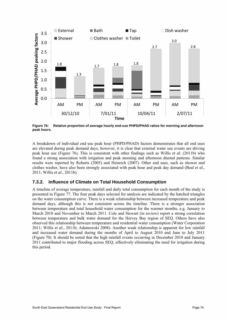
0.0
0.5
1.0
1.5
2.0
2.5
3.0
3.5
AM PM AM PM AM PM AM PM
30/12/10 7/01/11 10/04/11 2/07/11
Average PHPD/PHAD peaking factors
Time
External Bath Tap Dish washer
Shower Clothes washer Toilet
1.8
2.8
3.0
2.7
1.81.81.7
1.3
Figure 76: Relative proportion of average hourly end-use PHPD/PHAD ratios for morning and afternoon peak hours.
A breakdown of individual end use peak hour (PHPD/PHAD) factors demonstrates that all end uses are elevated during peak demand days, however, it is clear that external water use events are driving peak hour use (Figure 76). This is consistent with other findings such as Willis et al. (2011b) who found a strong association with irrigation and peak morning and afternoon diurnal patterns. Similar results were reported by Roberts (2005) and Heinrich (2007). Other end uses, such as shower and clothes washer, have also been strongly associated with peak hour and peak day demand (Beal et al., 2011; Willis et al., 2011b).
7.3.2. Influence of Climate on Total Household Consumption
A timeline of average temperature, rainfall and daily total consumption for each month of the study is presented in Figure 77. The four peak days selected for analysis are indicated by the hatched triangles on the water consumption curve. There is a weak relationship between increased temperature and peak demand days, although this is not consistent across the timeline. There is a stronger association between temperature and total household water consumption for the warmer months, e.g. January to March 2010 and November to March 2011. Cole and Stewart (in review) report a strong correlation between temperature and bulk water demand for the Hervey Bay region of SEQ. Others have also observed this relationship between temperature and residential water consumption (Water Corporation 2011; Willis et al., 2011b; Adamowski 2008). Another weak relationship is apparent for low rainfall and increased water demand during the months of April to August 2010 and June to July 2011 (Figure 70). It should be noted that the high rainfall events occurring in December 2010 and January 2011 contributed to major flooding across SEQ, effectively eliminating the need for irrigation during this period.
South East Queensland Residential End Use Study: Final Report Page 74
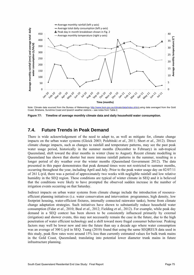
0
5
10
15
20
25
30
35
40
0
50
100
150
200
250
300
350
400
450
Average m
onthly temperature (C°)
Average m
onthly rainfall (m
m) an
d average total daily
water consumption (L/hh/d)
Time (months)
Average monthly rainfall (left y‐axis)
Average total daily consumption (left y‐axis)
Peak day in month breakdown shown in Fig. 2
Average monthly temperature (right y‐axis)
Note: Climate data sourced from the Bureau of Meteorology http://www.bom.gov.au/climate/data/index.shtml.using data averaged from the Gold Coast, Brisbane, Sunshine Coast and Ipswich weather stations – see notes from Table 2.
Figure 77: Timeline of average monthly climate data and daily household water consumption.
7.4. Future Trends in Peak Demand There is wide acknowledgement of the need to adapt to, as well as mitigate for, climate change impacts on the urban water systems (Gleick 2003; Polebitski et al., 2011; Short et al., 2012). Direct climate change impacts, such as changes to rainfall and temperature patterns, may see the past peak water usage period, historically in the summer months (December to February) in sub-tropical Queensland, shift toward the drier months in winter (June to August). Recent climate modelling in Queensland has shown that shorter but more intense rainfall patterns in the summer, resulting in a longer period of dry weather over the winter months (Queensland Government 2012). The data presented in this paper demonstrates that peak demand times were not restricted to summer months, occurring throughout the year, including April and July. Prior to the peak water usage day on 02/07/11 of 261 L/p/d, there was a period of approximately two weeks with negligible rainfall and low relative humidity in the SEQ region. These conditions are typical of winter climate in SEQ and it is believed that the conditions were likely to have prompted the observed sudden increase in the number of irrigation events occurring on that Saturday.
Indirect impacts on urban water systems from climate change include the introduction of resource-efficient planning initiatives (i.e. water conservation and intervention programmes, high density, low footprint housing, water-efficient fixtures, internally connected rainwater tanks), borne from climate change adaptation strategies. Such initiatives have shown to substantially reduce household water consumption (Fidar et al., 2010; Beal et al., 2012; Fielding et al., 2012). For example, while peak day demand in a SEQ context has been shown to be consistently influenced primarily by external (irrigation) and shower events, this may not necessarily remain the case in the future, due to the high penetration of water efficient technology and a shift toward more frugal consumer behaviour. Peaking factors may well be lower now and into the future than say a decade ago where water consumption was an average of 300 L/p/d in SEQ. Tsang (2010) found that using the same SEQREUS data used in this study, peak flow rates were around 15% less than currently estimated values for bulk trunk mains in the Gold Coast, Queensland; translating into potential lower diameter trunk mains in future infrastructure planning.
South East Queensland Residential End Use Study: Final Report Page 75
South East Queensland Residential End Use Study: Final Report Page 76
The effect of water efficient technology on daily diurnal patterns and peak flow is discussed by Carragher et al. (2012). They concluded strongly that the likely reductions in AD peak hour water demand is essentially inevitable given the mandate for all new dwellings to incorporate water efficiency stock (e.g. low-flow showers, water-efficient clothes washers and tap fixtures). Reduced peak day and peak hour demand due to residential water stock efficiency measures has implications for optimising pipe network modelling and capital infrastructure, e.g. deferral or reduction in water distribution infrastructure (Basupi et al., 2011; Carragher et al., 2012).
Irrigation has been shown to be dramatically reduced in the post-drought and post-water restriction environment in SEQ (Walton and Hume, 2010; Willis et al., 2011b; Beal et al., 2011). Further, three years post-drought, the expected rebound back to higher (e.g. >200 L/p/d) consumption is still not yet evident, despite the many months of above average rainfall which one would expect to encourage less frugal water use. Together with this water conservation behaviour, the residential landscape in SEQ has changed markedly over the years, with new developments being built on smaller allotment sizes, with reduced garden or lawn areas. Planning guidelines also strongly promote native species to be planted that require a lower frequency and volume of water. Due to recent local and global economic pressures; high density, smaller homes are often the affordable and thus the preferred dwelling type.
For various the reasons described above, household water consumption in SEQ is not likely to return to the daily capita usage of 300 L/p/d that was typical a decade ago. Consequently, the variation and volume of peak demand is also likely to change (decline). It is postulated that peak demand days will not only occur to a lesser degree, with lower incidences of high peaking factors in the future, but will also see a seasonal shift of high demand days from the warmer, wetter months to the cooler drier months. Some evidence of this has been presented herein, with lower daily and hourly peaking factors than historically reported, however, further analysis of the correlation between climate pattern and peak end usage based on an additional year of end use data is an important next step of this research.
7.5. Conclusions Information on hourly and daily peak demand at the end use level can facilitate the optimisation of infrastructure design and sizing and inform the subsequent deferral of such assets. The aim of this study was to determine peak hourly and daily demand for a range of water end uses in households located in SEQ. Peak day and peak hour demand was examined for four peak days identified from 18 months of empirical household water consumption data. Peak day demand that yielded peaking factors between 1 and 1.5 were observed to be primarily driven by clothes washer and shower use. However, as the peak day and peak hour demand rose above a PD/AD of 1.5, demand was strongly driven by external water usage.
Overall, peaking factors were lower than those being used in local planning guidelines for residential water supply. A reduction in the degree and frequency of peak demand days is likely due to the high penetration of residential water stock efficient measures, water consumer behavioural changes and anticipated changes to future climate patterns. Thus, caution should be exercised if using historic peak day and peak hour demand data for infrastructure design and modelling. This is especially pertinent in jurisdictions where factors influencing future water demand are evident, such as the wide incorporation of water efficient stock and permanent shifts in water conservation behaviours. Additionally, a shift to a winter peak demand for irrigation due the changes to seasonal rainfall patterns resulting from climate change is possible.
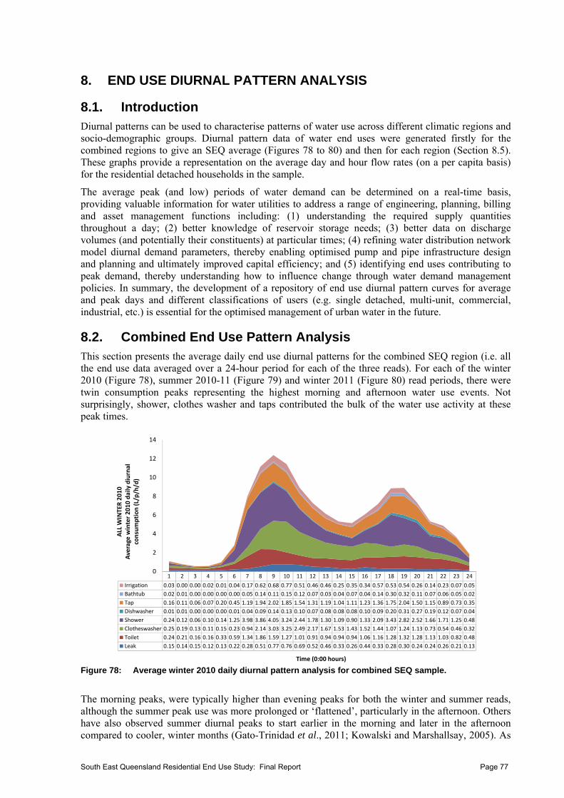
8. END USE DIURNAL PATTERN ANALYSIS
8.1. Introduction Diurnal patterns can be used to characterise patterns of water use across different climatic regions and socio-demographic groups. Diurnal pattern data of water end uses were generated firstly for the combined regions to give an SEQ average (Figures 78 to 80) and then for each region (Section 8.5). These graphs provide a representation on the average day and hour flow rates (on a per capita basis) for the residential detached households in the sample.
The average peak (and low) periods of water demand can be determined on a real-time basis, providing valuable information for water utilities to address a range of engineering, planning, billing and asset management functions including: (1) understanding the required supply quantities throughout a day; (2) better knowledge of reservoir storage needs; (3) better data on discharge volumes (and potentially their constituents) at particular times; (4) refining water distribution network model diurnal demand parameters, thereby enabling optimised pump and pipe infrastructure design and planning and ultimately improved capital efficiency; and (5) identifying end uses contributing to peak demand, thereby understanding how to influence change through water demand management policies. In summary, the development of a repository of end use diurnal pattern curves for average and peak days and different classifications of users (e.g. single detached, multi-unit, commercial, industrial, etc.) is essential for the optimised management of urban water in the future.
8.2. Combined End Use Pattern Analysis This section presents the average daily end use diurnal patterns for the combined SEQ region (i.e. all the end use data averaged over a 24-hour period for each of the three reads). For each of the winter 2010 (Figure 78), summer 2010-11 (Figure 79) and winter 2011 (Figure 80) read periods, there were twin consumption peaks representing the highest morning and afternoon water use events. Not surprisingly, shower, clothes washer and taps contributed the bulk of the water use activity at these peak times.
1 2 3 4 5 6 7 8 9 10 11 12 13 14 15 16 17 18 19 20 21 22 23 24
Irrigation 0.03 0.00 0.00 0.02 0.01 0.04 0.17 0.62 0.68 0.77 0.51 0.46 0.46 0.25 0.35 0.34 0.57 0.53 0.54 0.26 0.14 0.23 0.07 0.05
Bathtub 0.02 0.01 0.00 0.00 0.00 0.00 0.05 0.14 0.11 0.15 0.12 0.07 0.03 0.04 0.07 0.04 0.14 0.30 0.32 0.11 0.07 0.06 0.05 0.02
Tap 0.16 0.11 0.06 0.07 0.20 0.45 1.19 1.94 2.02 1.85 1.54 1.31 1.19 1.04 1.11 1.23 1.36 1.75 2.04 1.50 1.15 0.89 0.73 0.35
Dishwasher 0.01 0.01 0.00 0.00 0.00 0.01 0.04 0.09 0.14 0.13 0.10 0.07 0.08 0.08 0.08 0.10 0.09 0.20 0.31 0.27 0.19 0.12 0.07 0.04
Shower 0.24 0.12 0.06 0.10 0.14 1.25 3.98 3.86 4.05 3.24 2.44 1.78 1.30 1.09 0.90 1.33 2.09 3.43 2.82 2.52 1.66 1.71 1.25 0.48
Clotheswasher 0.25 0.19 0.13 0.11 0.15 0.23 0.94 2.14 3.03 3.25 2.49 2.17 1.67 1.53 1.43 1.52 1.44 1.07 1.24 1.13 0.73 0.54 0.46 0.32
Toilet 0.24 0.21 0.16 0.16 0.33 0.59 1.34 1.86 1.59 1.27 1.01 0.91 0.94 0.94 0.94 1.06 1.16 1.28 1.32 1.28 1.13 1.03 0.82 0.48
Leak 0.15 0.14 0.15 0.12 0.13 0.22 0.28 0.51 0.77 0.76 0.69 0.52 0.46 0.33 0.26 0.44 0.33 0.28 0.30 0.24 0.24 0.26 0.21 0.13
0
2
4
6
8
10
12
14
ALL W
INTER 2010
Average winter 2010 daily diurnal
consumption (L/p/h/d)
Time (0:00 hours) Figure 78: Average winter 2010 daily diurnal pattern analysis for combined SEQ sample.
The morning peaks, were typically higher than evening peaks for both the winter and summer reads, although the summer peak use was more prolonged or ‘flattened’, particularly in the afternoon. Others have also observed summer diurnal peaks to start earlier in the morning and later in the afternoon compared to cooler, winter months (Gato-Trinidad et al., 2011; Kowalski and Marshallsay, 2005). As
South East Queensland Residential End Use Study: Final Report Page 77
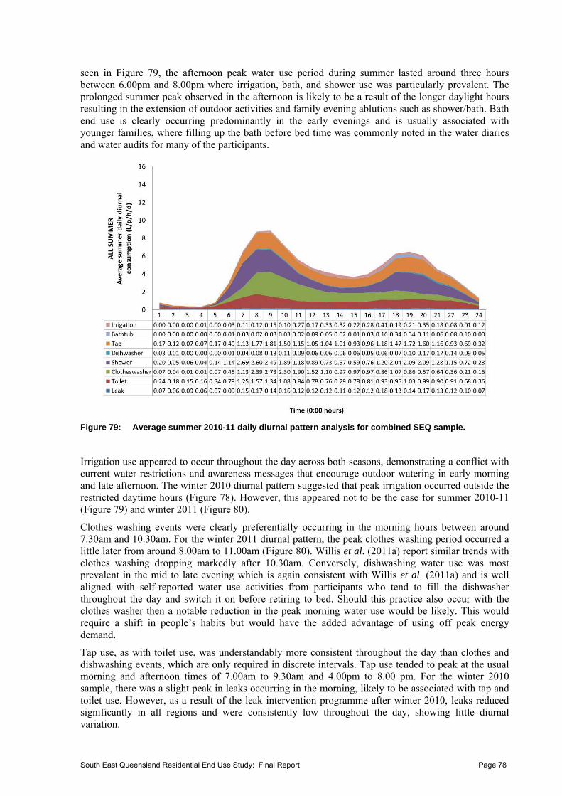
seen in Figure 79, the afternoon peak water use period during summer lasted around three hours between 6.00pm and 8.00pm where irrigation, bath, and shower use was particularly prevalent. The prolonged summer peak observed in the afternoon is likely to be a result of the longer daylight hours resulting in the extension of outdoor activities and family evening ablutions such as shower/bath. Bath end use is clearly occurring predominantly in the early evenings and is usually associated with younger families, where filling up the bath before bed time was commonly noted in the water diaries and water audits for many of the participants.
Figure 79: Average summer 2010-11 daily diurnal pattern analysis for combined SEQ sample.
Irrigation use appeared to occur throughout the day across both seasons, demonstrating a conflict with current water restrictions and awareness messages that encourage outdoor watering in early morning and late afternoon. The winter 2010 diurnal pattern suggested that peak irrigation occurred outside the restricted daytime hours (Figure 78). However, this appeared not to be the case for summer 2010-11 (Figure 79) and winter 2011 (Figure 80).
Clothes washing events were clearly preferentially occurring in the morning hours between around 7.30am and 10.30am. For the winter 2011 diurnal pattern, the peak clothes washing period occurred a little later from around 8.00am to 11.00am (Figure 80). Willis et al. (2011a) report similar trends with clothes washing dropping markedly after 10.30am. Conversely, dishwashing water use was most prevalent in the mid to late evening which is again consistent with Willis et al. (2011a) and is well aligned with self-reported water use activities from participants who tend to fill the dishwasher throughout the day and switch it on before retiring to bed. Should this practice also occur with the clothes washer then a notable reduction in the peak morning water use would be likely. This would require a shift in people’s habits but would have the added advantage of using off peak energy demand.
Tap use, as with toilet use, was understandably more consistent throughout the day than clothes and dishwashing events, which are only required in discrete intervals. Tap use tended to peak at the usual morning and afternoon times of 7.00am to 9.30am and 4.00pm to 8.00 pm. For the winter 2010 sample, there was a slight peak in leaks occurring in the morning, likely to be associated with tap and toilet use. However, as a result of the leak intervention programme after winter 2010, leaks reduced significantly in all regions and were consistently low throughout the day, showing little diurnal variation.
South East Queensland Residential End Use Study: Final Report Page 78
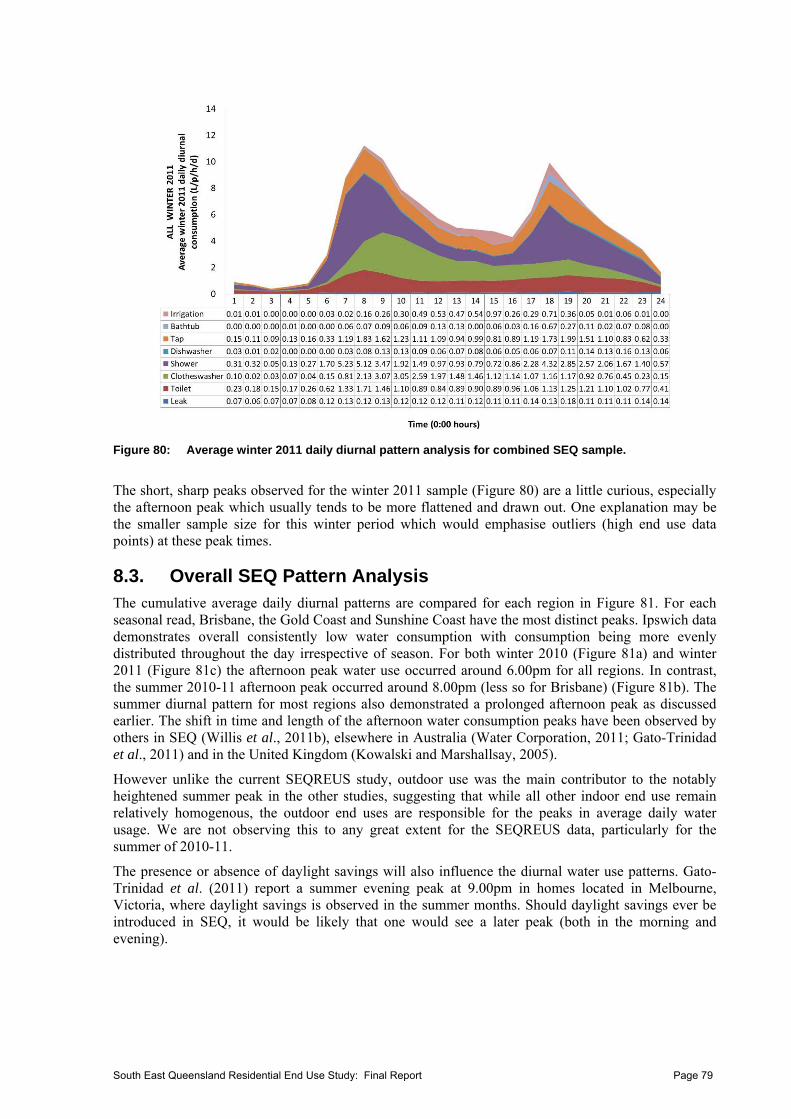
Figure 80: Average winter 2011 daily diurnal pattern analysis for combined SEQ sample.
The short, sharp peaks observed for the winter 2011 sample (Figure 80) are a little curious, especially the afternoon peak which usually tends to be more flattened and drawn out. One explanation may be the smaller sample size for this winter period which would emphasise outliers (high end use data points) at these peak times.
8.3. Overall SEQ Pattern Analysis The cumulative average daily diurnal patterns are compared for each region in Figure 81. For each seasonal read, Brisbane, the Gold Coast and Sunshine Coast have the most distinct peaks. Ipswich data demonstrates overall consistently low water consumption with consumption being more evenly distributed throughout the day irrespective of season. For both winter 2010 (Figure 81a) and winter 2011 (Figure 81c) the afternoon peak water use occurred around 6.00pm for all regions. In contrast, the summer 2010-11 afternoon peak occurred around 8.00pm (less so for Brisbane) (Figure 81b). The summer diurnal pattern for most regions also demonstrated a prolonged afternoon peak as discussed earlier. The shift in time and length of the afternoon water consumption peaks have been observed by others in SEQ (Willis et al., 2011b), elsewhere in Australia (Water Corporation, 2011; Gato-Trinidad et al., 2011) and in the United Kingdom (Kowalski and Marshallsay, 2005).
However unlike the current SEQREUS study, outdoor use was the main contributor to the notably heightened summer peak in the other studies, suggesting that while all other indoor end use remain relatively homogenous, the outdoor end uses are responsible for the peaks in average daily water usage. We are not observing this to any great extent for the SEQREUS data, particularly for the summer of 2010-11.
The presence or absence of daylight savings will also influence the diurnal water use patterns. Gato-Trinidad et al. (2011) report a summer evening peak at 9.00pm in homes located in Melbourne, Victoria, where daylight savings is observed in the summer months. Should daylight savings ever be introduced in SEQ, it would be likely that one would see a later peak (both in the morning and evening).
South East Queensland Residential End Use Study: Final Report Page 79
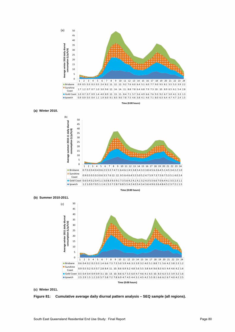
1 2 3 4 5 6 7 8 9 10 11 12 13 14 15 16 17 18 19 20 21 22 23 24
Brisbane 0.9 0.5 0.3 0.3 0.5 2.4 8.2 11. 12. 12. 9.2 7.6 6.0 6.4 5.1 6.0 7.7 9.0 9.5 8.1 5.5 5.3 3.9 2.2
SunshineCoast
1.7 1.2 0.7 0.7 1.0 3.0 9.6 12. 14. 14. 11. 8.8 7.8 6.4 6.8 7.9 7.3 10. 10. 8.9 6.5 6.1 5.4 2.8
Gold Coast 1.0 0.7 0.7 0.9 1.4 4.0 8.9 12. 13. 11. 8.4 7.1 5.7 5.6 4.9 6.6 7.6 9.3 9.2 6.7 5.0 4.1 3.3 1.3
Ipswich 0.9 0.9 0.5 0.4 1.1 1.9 6.0 9.1 8.5 9.0 7.8 7.5 4.6 3.8 4.1 4.6 7.1 8.0 6.3 6.4 4.7 4.7 2.4 1.5
0
5
10
15
20
25
30
35
40
45
50
Average
winter 2010 daily diurnal
consumption (L/p/h/d)
Time (0:00 hours)
(a)
(a) Winter 2010.
1 2 3 4 5 6 7 8 9 10 11 12 13 14 15 16 17 18 19 20 21 22 23 24
Brisbane 0.7 0.3 0.4 0.4 0.6 2.5 5.5 7.4 7.1 6.4 6.1 4.5 3.8 3.4 3.3 3.8 4.5 6.3 6.4 5.1 4.5 3.4 2.2 1.0
SunshineCoast
0.9 0.5 0.5 0.3 0.6 3.5 7.6 12. 12. 9.5 6.4 6.4 5.5 5.0 5.2 4.7 5.9 7.3 7.5 6.7 5.3 5.1 4.0 2.4
Gold Coast 0.6 0.4 0.2 0.4 1.1 3.0 8.3 9.3 9.1 7.3 5.6 4.2 4.1 4.1 3.2 4.3 5.5 6.6 7.0 6.4 4.1 3.5 2.3 1.1
Ipswich 1.2 1.0 0.7 0.5 1.1 4.1 5.5 7.2 8.7 6.8 5.5 4.2 4.0 3.4 3.4 3.6 4.9 6.3 6.4 8.4 5.2 3.7 2.1 1.5
0
5
10
15
20
25
30
35
40
45
50
Average summer 2010‐11 daily diurnal
consumption (L/p/h/d)
Time (0:00 hours)
(b)
(b) Summer 2010-2011.
1 2 3 4 5 6 7 8 9 10 11 12 13 14 15 16 17 18 19 20 21 22 23 24
Brisbane 0.6 0.4 0.2 0.2 0.3 1.4 6.6 7.3 7.3 5.0 5.9 4.6 3.3 3.9 3.2 4.0 5.1 8.8 7.1 5.6 4.2 3.8 2.3 1.2
SunshineCoast
0.9 0.5 0.2 0.3 0.7 2.8 8.4 11. 10. 8.6 6.9 6.2 4.8 5.6 5.5 3.8 6.4 9.6 8.3 6.5 4.4 4.6 4.2 1.6
Gold Coast 0.5 0.4 0.4 0.9 0.9 3.1 10. 13. 10. 8.6 6.7 5.5 6.0 4.7 4.6 4.1 6.5 10. 8.3 6.3 5.5 3.9 3.2 1.6
Ipswich 2.5 2.9 1.5 1.2 2.0 5.7 5.8 7.2 7.8 6.9 4.7 4.5 4.4 3.1 4.5 4.2 5.5 8.1 6.6 6.2 6.7 4.0 4.2 2.5
0
5
10
15
20
25
30
35
40
45
50
Average winter 2011 daily diurnal
consumption (L/p/h/d)
Time (0:00 hours)
(c)
(c) Winter 2011.
Figure 81: Cumulative average daily diurnal pattern analysis – SEQ sample (all regions).
South East Queensland Residential End Use Study: Final Report Page 80
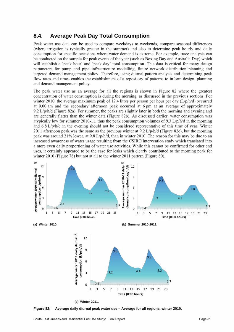
8.4. Average Peak Day Total Consumption Peak water use data can be used to compare weekdays to weekends, compare seasonal differences (where irrigation is typically greater in the summer) and also to determine peak hourly and daily consumption for specific occasions where water demand is extreme. For example, trace analysis can be conducted on the sample for peak events of the year (such as Boxing Day and Australia Day) which will establish a ‘peak hour’ and ‘peak day’ total consumption. This data is critical for many design parameters for pump and pipe infrastructure modelling, future network distribution planning and targeted demand management policy. Therefore, using diurnal pattern analysis and determining peak flow rates and times enables the establishment of a repository of patterns to inform design, planning and demand management policy.
The peak water use as an average for all the regions is shown in Figure 82 where the greatest concentration of water consumption is during the morning, as discussed in the previous sections. For winter 2010, the average maximum peak of 12.4 litres per person per hour per day (L/p/h/d) occurred at 9.00 am and the secondary afternoon peak occurred at 6 pm at an average of approximately 9.2 L/p/h/d (Figure 82a). For summer, the peaks are slightly later in both the morning and evening and are generally flatter than the winter data (Figure 82b). As discussed earlier, water consumption was atypically low for summer 2010-11, thus the peak consumption volumes of 9.3 L/p/h/d in the morning and 6.8 L/p/h/d in the evening should not be considered representative of this time of year. Winter 2011 afternoon peak was the same as the previous winter at 9.2 L/p/h/d (Figure 82c), but the morning peak was around 21% lower, at 9.8 L/p/h/d, than in winter 2010. The reason for this may be due to an increased awareness of water usage resulting from the CSIRO intervention study which translated into a more even daily proportioning of water use activities. While this cannot be confirmed for other end uses, it certainly appeared to be the case for leaks which clearly contributed to the morning peak for winter 2010 (Figure 78) but not at all to the winter 2011 pattern (Figure 80).
(a) Winter 2010. (b) Summer 2010-2011.
(c) Winter 2011.
Figure 82: Average daily diurnal peak water use – Average for all regions, winter 2010.
South East Queensland Residential End Use Study: Final Report Page 81
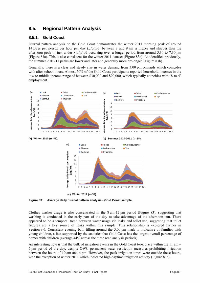
8.5. Regional Pattern Analysis
8.5.1. Gold Coast
Diurnal pattern analysis on the Gold Coast demonstrates the winter 2011 morning peak of around 14 litres per person per hour per day (L/p/h/d) between 8 and 9 am is higher and sharper than the afternoon peak of just under 8 L/p/h/d occurring over a longer period from around 5.30 to 7.30 pm (Figure 83a). This is also consistent for the winter 2011 dataset (Figure 83c). As identified previously, the summer 2010-11 peaks are lower and later and generally more prolonged (Figure 83b).
Generally, there is a clear and steady rise in water demand from 3.00 pm onwards which coincides with after school hours. Almost 50% of the Gold Coast participants reported household incomes in the low to middle income range of between $30,000 and $90,000, which typically coincides with ‘8-to-5’ employment.
0
2
4
6
8
10
12
14
1 2 3 4 5 6 7 8 9 10 11 12 13 14 15 16 17 18 19 20 21 22 23 24
Average
daily diurnal consumption
(L/p/h/d)
Leak Toilet Clotheswasher
Shower Dishwasher Tap
Bathtub Irrigation
(a)
0
2
4
6
8
10
12
14
1 2 3 4 5 6 7 8 9 10 11 12 13 14 15 16 17 18 19 20 21 22 23 24Average
daily diurnal consumption
(L/p/h/d)
Leak Toilet Clotheswasher
Shower Dishwasher Tap
Bathtub Irrigation
(b)
(a) Winter 2010 (n=87). (b) Summer 2010-2011 (n=68).
0
2
4
6
8
10
12
14
1 2 3 4 5 6 7 8 9 10 11 12 13 14 15 16 17 18 19 20 21 22 23 24Average
daily diurnal consumption
(L/p/h/d)
Leak Toilet Clotheswasher
Shower Dishwasher Tap
Bathtub Irrigation
(c)
(c) Winter 2011 (n=33).
Figure 83: Average daily diurnal pattern analysis - Gold Coast sample.
Clothes washer usage is also concentrated in the 8 am-12 pm period (Figure 83), suggesting that washing is conducted in the early part of the day to take advantage of the afternoon sun. There appeared to be a temporal trend between water usage via leaks and toilet use, suggesting that toilet fixtures are a key source of leaks within this sample. This relationship is explored further in Section 9.6. Consistent evening bath filling around the 5.00 pm mark is indicative of families with young children, a fact supported by the statistics that Gold Coast has the largest overall percentage of homes with children (average 44% across the three read analysis periods).
An interesting note is that the bulk of irrigation events in the Gold Coast took place within the 11 am – 5 pm period of the day, despite QWC permanent water restriction measures prohibiting irrigation between the hours of 10 am and 4 pm. However, the peak irrigation times were outside these hours, with the exception of winter 2011 which indicated high daytime irrigation activity (Figure 83c).
South East Queensland Residential End Use Study: Final Report Page 82
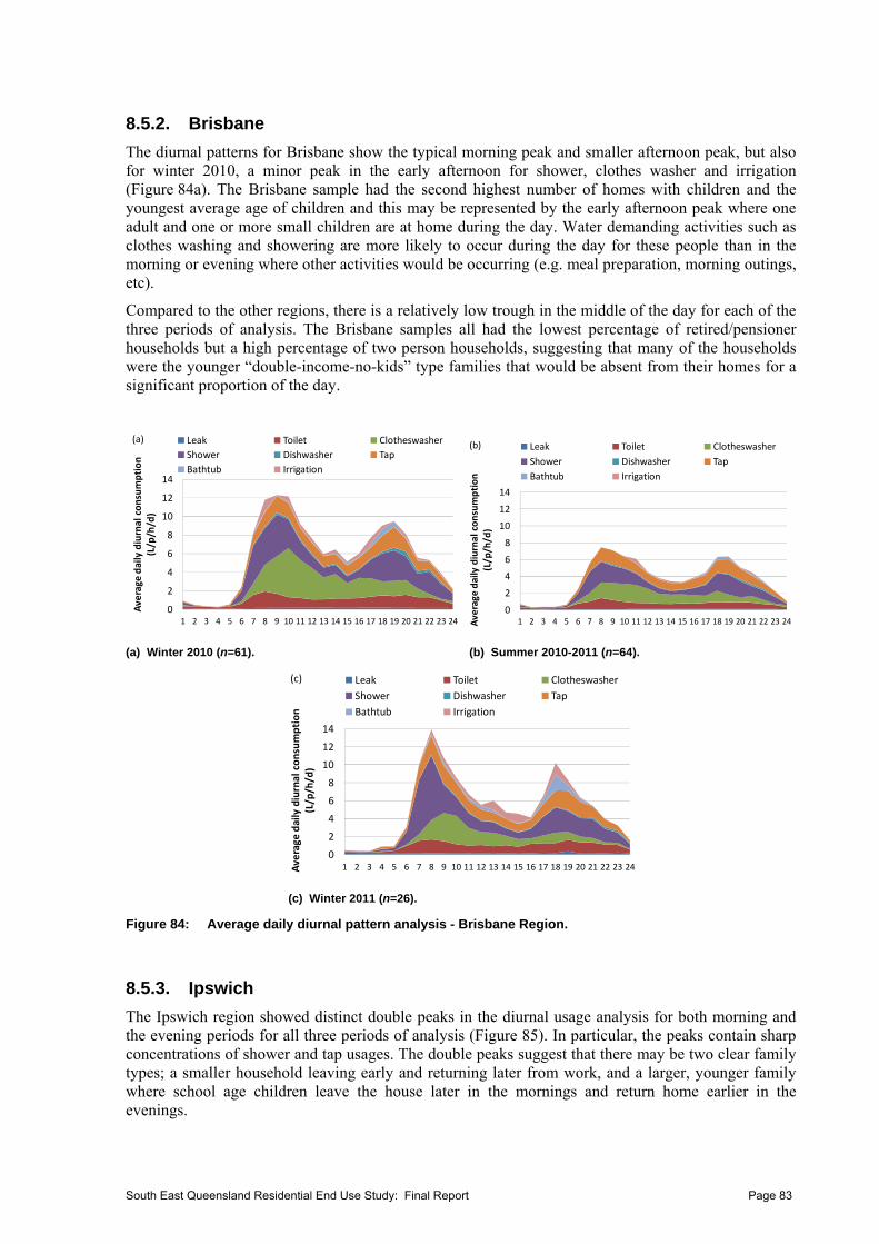
8.5.2. Brisbane
The diurnal patterns for Brisbane show the typical morning peak and smaller afternoon peak, but also for winter 2010, a minor peak in the early afternoon for shower, clothes washer and irrigation (Figure 84a). The Brisbane sample had the second highest number of homes with children and the youngest average age of children and this may be represented by the early afternoon peak where one adult and one or more small children are at home during the day. Water demanding activities such as clothes washing and showering are more likely to occur during the day for these people than in the morning or evening where other activities would be occurring (e.g. meal preparation, morning outings, etc).
Compared to the other regions, there is a relatively low trough in the middle of the day for each of the three periods of analysis. The Brisbane samples all had the lowest percentage of retired/pensioner households but a high percentage of two person households, suggesting that many of the households were the younger “double-income-no-kids” type families that would be absent from their homes for a significant proportion of the day.
0
2
4
6
8
10
12
14
1 2 3 4 5 6 7 8 9 10 11 12 13 14 15 16 17 18 19 20 21 22 23 24
Average
daily diurnal consumption
(L/p/h/d)
Leak Toilet Clotheswasher
Shower Dishwasher Tap
Bathtub Irrigation
(a)
0
2
4
6
8
10
12
14
1 2 3 4 5 6 7 8 9 10 11 12 13 14 15 16 17 18 19 20 21 22 23 24Average
daily diurnal consumption
(L/p/h/d)
Leak Toilet Clotheswasher
Shower Dishwasher Tap
Bathtub Irrigation
(b)
(a) Winter 2010 (n=61). (b) Summer 2010-2011 (n=64).
0
2
4
6
8
10
12
14
1 2 3 4 5 6 7 8 9 10 11 12 13 14 15 16 17 18 19 20 21 22 23 24Average
daily diurnal consumption
(L/p/h/d)
Leak Toilet Clotheswasher
Shower Dishwasher Tap
Bathtub Irrigation
(c)
(c) Winter 2011 (n=26).
Figure 84: Average daily diurnal pattern analysis - Brisbane Region.
8.5.3. Ipswich
The Ipswich region showed distinct double peaks in the diurnal usage analysis for both morning and the evening periods for all three periods of analysis (Figure 85). In particular, the peaks contain sharp concentrations of shower and tap usages. The double peaks suggest that there may be two clear family types; a smaller household leaving early and returning later from work, and a larger, younger family where school age children leave the house later in the mornings and return home earlier in the evenings.
South East Queensland Residential End Use Study: Final Report Page 83
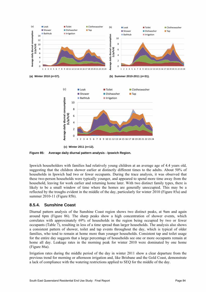
0
2
4
6
8
10
12
14
1 2 3 4 5 6 7 8 9 10 11 12 13 14 15 16 17 18 19 20 21 22 23 24
Average
daily diurnal consumption
(L/p/h/d)
Leak Toilet Clotheswasher
Shower Dishwasher Tap
Bathtub Irrigation
(a)
0
2
4
6
8
10
1 2 3 4 5 6 7 8 9 10 11 12 13 14 15 16 17 18 19 20 21 22 23 24Average
daily diurnal consumption
(L/p/h/d)
Leak Toilet Clotheswasher
Shower Dishwasher Tap
Bathtub Irrigation
(b)
(a) Winter 2010 (n=37). (b) Summer 2010-2011 (n=31).
0
2
4
6
8
10
1 2 3 4 5 6 7 8 9 10 11 12 13 14 15 16 17 18 19 20 21 22 23 24Average
daily diurnal consumption
(L/p/h/d)
Leak Toilet Clotheswasher
Shower Dishwasher Tap
Bathtub Irrigation
(c)
(c) Winter 2011 (n=12).
Figure 85: Average daily diurnal pattern analysis - Ipswich Region.
Ipswich householders with families had relatively young children at an average age of 4.4 years old, suggesting that the children shower earlier at distinctly different times to the adults. About 50% of households in Ipswich had two or fewer occupants. During the trace analysis, it was observed that these two-person households were typically younger, and appeared to spend more time away from the household, leaving for work earlier and returning home later. With two distinct family types, there is likely to be a small window of time where the homes are generally unoccupied. This may be a reflected by the troughs evident in the middle of the day, particularly for winter 2010 (Figure 85a) and summer 2010-11 (Figure 85b).
8.5.4. Sunshine Coast
Diurnal pattern analysis of the Sunshine Coast region shows two distinct peaks, at 9am and again around 6pm (Figure 86). The sharp peaks show a high concentration of shower events, which correlates with approximately 69% of households in the region being occupied by two or fewer occupants (Table 7), resulting in less of a time spread than larger households. The analysis also shows a consistent pattern of shower, toilet and tap events throughout the day, which is typical of older families, who tend to remain at home more than younger households. Consistent tap and toilet usage for the entire day suggests that a large percentage of households see one or more occupants remain at home all day. Leakage rates in the morning peak for winter 2010 were dominated by one home (Figure 86a).
Irrigation rates during the middle period of the day in winter 2011 show a clear departure from the previous trend for morning or afternoon irrigation and, like Brisbane and the Gold Coast, demonstrate a lack of compliance with the watering restrictions applied to SEQ for the middle of the day.
South East Queensland Residential End Use Study: Final Report Page 84
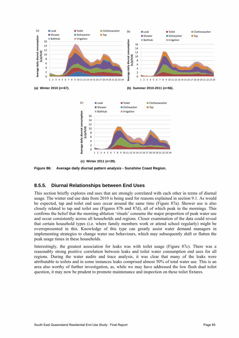
0
2
4
6
8
10
12
14
16
1 2 3 4 5 6 7 8 9 10 11 12 13 14 15 16 17 18 19 20 21 22 23 24
Average
daily diurnal consumption
(L/p/h/d)
Leak Toilet Clotheswasher
Shower Dishwasher Tap
Bathtub Irrigation
(a)
0
2
4
6
8
10
12
14
16
1 2 3 4 5 6 7 8 9 10 11 12 13 14 15 16 17 18 19 20 21 22 23 24Average
daily diurnal consumption
(L/p/h/d)
Leak Toilet Clotheswasher
Shower Dishwasher Tap
Bathtub Irrigation
(b)
(a) Winter 2010 (n=67). (b) Summer 2010-2011 (n=56).
0
2
4
6
8
10
12
14
16
1 2 3 4 5 6 7 8 9 10 11 12 13 14 15 16 17 18 19 20 21 22 23 24Average
daily diurnal consumption
(L/p/h/d)
Leak Toilet Clotheswasher
Shower Dishwasher Tap
Bathtub Irrigation
(c)
(c) Winter 2011 (n=39).
Figure 86: Average daily diurnal pattern analysis - Sunshine Coast Region.
8.5.5. Diurnal Relationships between End Uses
This section briefly explores end uses that are strongly correlated with each other in terms of diurnal usage. The winter end use data from 2010 is being used for reasons explained in section 9.1. As would be expected, tap and toilet end uses occur around the same time (Figure 87a). Shower use is also closely related to tap and toilet use (Figures 87b and 87d), all of which peak in the mornings. This confirms the belief that the morning ablution ‘rituals’ consume the major proportion of peak water use and occur consistently across all households and regions. Closer examination of the data could reveal that certain household types (i.e. where family members work or attend school regularly) might be overrepresented in this. Knowledge of this type can greatly assist water demand managers in implementing strategies to change water use behaviours, which may subsequently shift or flatten the peak usage times in these households.
Interestingly, the greatest association for leaks was with toilet usage (Figure 87c). There was a reasonably strong positive correlation between leaks and toilet water consumption end uses for all regions. During the water audits and trace analysis, it was clear that many of the leaks were attributable to toilets and in some instances leaks comprised almost 50% of total water use. This is an area also worthy of further investigation, as, while we may have addressed the low flush dual toilet question, it may now be prudent to promote maintenance and inspection on these toilet fixtures.
South East Queensland Residential End Use Study: Final Report Page 85
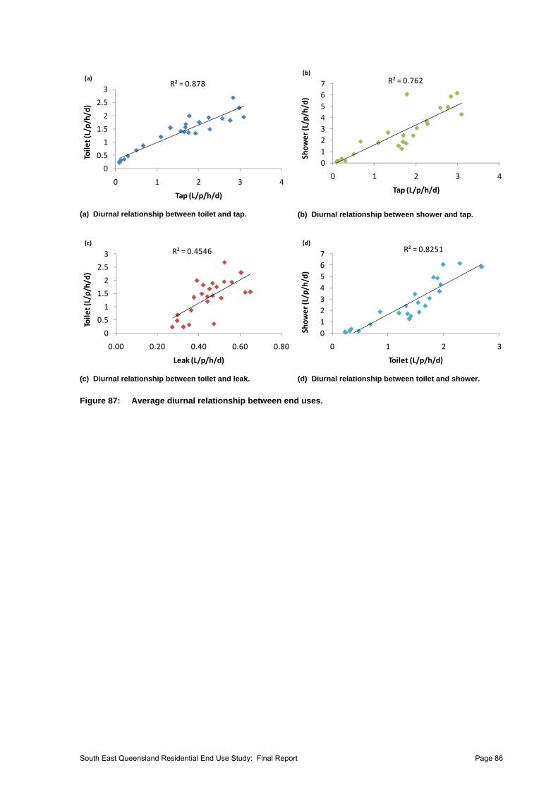
R² = 0.878
0
0.5
1
1.5
2
2.5
3
0 1 2 3 4
Toilet (L/p/h/d)
Tap (L/p/h/d)
(a)
(a) Diurnal relationship between toilet and tap.
R² = 0.762
0
1
2
3
4
5
6
7
0 1 2 3 4
Shower (L/p/h/d)
Tap (L/p/h/d)
(b)
(b) Diurnal relationship between shower and tap.
R² = 0.4546
0
0.5
1
1.5
2
2.5
3
0.00 0.20 0.40 0.60 0.80
Toilet (L/p/h/d)
Leak (L/p/h/d)
(c)
(c) Diurnal relationship between toilet and leak.
R² = 0.8251
0
1
2
3
4
5
6
7
0 1 2 3
Shower (L/p/h/d)
Toilet (L/p/h/d)
(d)
(d) Diurnal relationship between toilet and shower.
Figure 87: Average diurnal relationship between end uses.
South East Queensland Residential End Use Study: Final Report Page 86
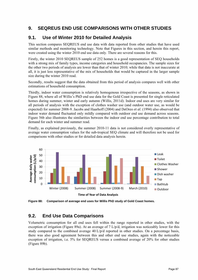
9. SEQREUS END USE COMPARISONS WITH OTHER STUDIES
9.1. Use of Winter 2010 for Detailed Analysis This section compares SEQREUS end use data with data reported from other studies that have used similar methods and monitoring technology. Note that Figures in this section, and herein this report, were created using the winter 2010 end use data only. There are several reasons for this.
Firstly, the winter 2010 SEQREUS sample of 252 homes is a good representation of SEQ households with a strong mix of family types, income categories and household occupancies. The sample sizes for the other two periods of analysis are lower than that of winter 2010; while that data is not inaccurate at all, it is just less representative of the mix of households that would be captured in the larger sample size during the winter 2010 read.
Secondly, results suggest that the data obtained from this period of analysis compares well with other estimations of household consumption.
Thirdly, indoor water consumption is relatively homogenous irrespective of the seasons, as shown in Figure 88, where all of Willis’s PhD end use data for the Gold Coast is presented for single reticulated homes during summer, winter and early autumn (Willis, 2011d). Indoor end uses are very similar for all periods of analysis with the exception of clothes washer use (and outdoor water use, as would be expected) for summer 2008-9. Jacobs and Haarhoff (2004) and DeOreo et al. (1994) also observed that indoor water demand fluctuated only mildly compared with outdoor end use demand across seasons. Figure 56b also illustrates the similarities between the indoor end use percentage contribution to total demand for each winter and summer read.
Finally, as explained previously, the summer 2010-11 data is not considered overly representative of average water consumption values for the sub-tropical SEQ climate and will therefore not be used for comparisons with other studies or for detailed data analysis herein.
0
10
20
30
40
50
60
Winter (2008) Summer (2008) Summer (2008‐9) March (2010)
Average daily water
consumption (L/p/d)
Time of Year of Data Analysis
Leak
Toilet
Clothes Washer
Shower
Dish washer
Tap
Bathtub
Outdoor
Figure 88: Comparison of average end uses for Willis PhD study of Gold Coast homes.
9.2. End Use Data Comparisons Volumetric consumption for all end uses fell within the range reported in other studies, with the exception of irrigation (Figure 89a). At an average of 7 L/p/d, irrigation was noticeably lower for this study compared to the combined average 40 L/p/d reported in other studies. On a percentage basis, there was also good agreement between this and other end use studies, again with the noticeable exception of irrigation, i.e. 5% for SEQREUS versus a combined average of 20% for other studies (Figure 89b).
South East Queensland Residential End Use Study: Final Report Page 87
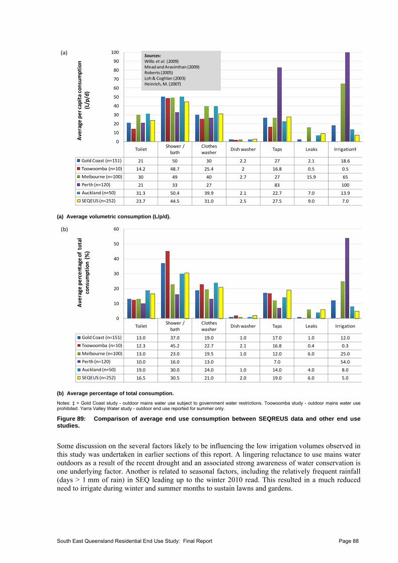
ToiletShower /
bath
Clothes
washerDish washer Taps Leaks Irrigation‡
Gold Coast (n=151) 21 50 30 2.2 27 2.1 18.6
Toowoomba (n=10) 14.2 48.7 25.4 2 16.8 0.5 0.5
Melbourne (n=100) 30 49 40 2.7 27 15.9 65
Perth (n=120) 21 33 27 83 100
Auckland (n=50) 31.3 50.4 39.9 2.1 22.7 7.0 13.9
SEQEUS (n=252) 23.7 44.5 31.0 2.5 27.5 9.0 7.0
0
10
20
30
40
50
60
70
80
90
100
Average per capita consumption
(L/p/d)
Sources: Willis et al. (2009)Mead and Aravinthan (2009)Roberts (2005)Loh & Coghlan (2003)Heinrich, M. (2007)
(a)
(a) Average volumetric consumption (L/p/d).
ToiletShower / bath
Clothes washer
Dish washer Taps Leaks Irrigation
Gold Coast (n=151) 13.0 37.0 19.0 1.0 17.0 1.0 12.0
Toowoomba (n=10) 12.3 45.2 22.7 2.1 16.8 0.4 0.3
Melbourne (n=100) 13.0 23.0 19.5 1.0 12.0 6.0 25.0
Perth (n=120) 10.0 16.0 13.0 7.0 54.0
Auckland (n=50) 19.0 30.0 24.0 1.0 14.0 4.0 8.0
SEQEUS (n=252) 16.5 30.5 21.0 2.0 19.0 6.0 5.0
0
10
20
30
40
50
60
Average percentage of total
consumption (%)
(b)
(b) Average percentage of total consumption.
Notes: ‡ = Gold Coast study - outdoor mains water use subject to government water restrictions. Toowoomba study - outdoor mains water use prohibited. Yarra Valley Water study - outdoor end use reported for summer only.
Figure 89: Comparison of average end use consumption between SEQREUS data and other end use studies.
Some discussion on the several factors likely to be influencing the low irrigation volumes observed in this study was undertaken in earlier sections of this report. A lingering reluctance to use mains water outdoors as a result of the recent drought and an associated strong awareness of water conservation is one underlying factor. Another is related to seasonal factors, including the relatively frequent rainfall (days > 1 mm of rain) in SEQ leading up to the winter 2010 read. This resulted in a much reduced need to irrigate during winter and summer months to sustain lawns and gardens.
South East Queensland Residential End Use Study: Final Report Page 88
South East Queensland Residential End Use Study: Final Report Page 89
As for previous studies, shower usage comprised the bulk of household water use for all regions. Across all regions, a minimum of one quarter of all household water demand was associated with this practice. This is not unusual and has been reported in other end use studies (Willis et al., 2010b, 2011a; Gato-Trinidad et al., 2011; Water Corporation, 2011; Mead and Aravinthan, 2009).
Leakage rates for the SEQREUS are consistent with other studies both on a volumetric and percentage basis (Figure 89). Leaks are a common occurrence in all households, with a trend typically shown for less leakage to occur from new (< five years old) dwellings (Willis et al., 2009a). For the SEQREUS winter 2010 sample, leaks ranged from 0.2 to 513 L/p/d. The latter value is an extreme case and subsequent investigation has revealed that this household has had ongoing issues with leaks on its property. Very large leaks are usually due to service breaks and can cause the average per capita leakage volumes in an end use sample to fluctuate significantly. Leakage rates for the subsequent summer 2010-11 and winter 2011 were substantially reduced as a result of the aligned CSIRO intervention study as discussed previously.
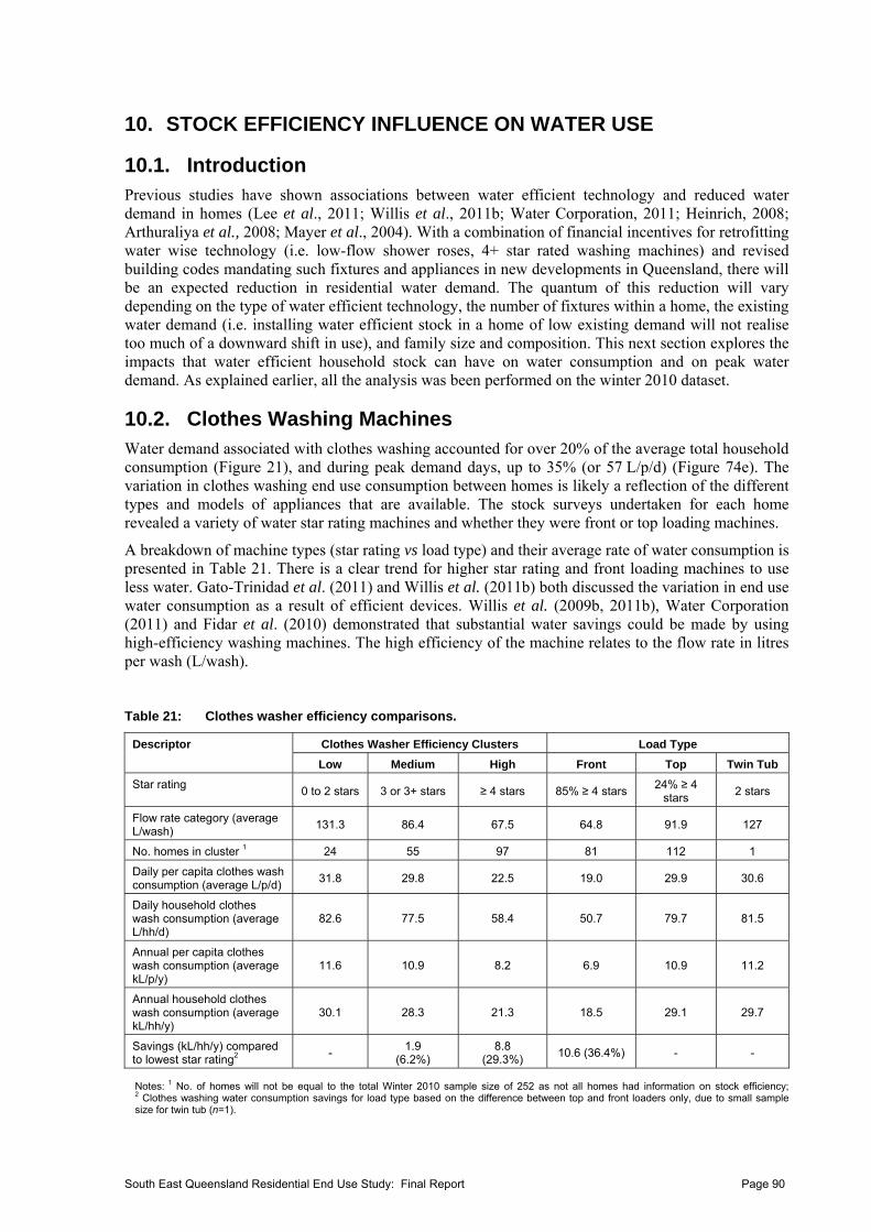
10. STOCK EFFICIENCY INFLUENCE ON WATER USE
10.1. Introduction Previous studies have shown associations between water efficient technology and reduced water demand in homes (Lee et al., 2011; Willis et al., 2011b; Water Corporation, 2011; Heinrich, 2008; Arthuraliya et al., 2008; Mayer et al., 2004). With a combination of financial incentives for retrofitting water wise technology (i.e. low-flow shower roses, 4+ star rated washing machines) and revised building codes mandating such fixtures and appliances in new developments in Queensland, there will be an expected reduction in residential water demand. The quantum of this reduction will vary depending on the type of water efficient technology, the number of fixtures within a home, the existing water demand (i.e. installing water efficient stock in a home of low existing demand will not realise too much of a downward shift in use), and family size and composition. This next section explores the impacts that water efficient household stock can have on water consumption and on peak water demand. As explained earlier, all the analysis was been performed on the winter 2010 dataset.
10.2. Clothes Washing Machines Water demand associated with clothes washing accounted for over 20% of the average total household consumption (Figure 21), and during peak demand days, up to 35% (or 57 L/p/d) (Figure 74e). The variation in clothes washing end use consumption between homes is likely a reflection of the different types and models of appliances that are available. The stock surveys undertaken for each home revealed a variety of water star rating machines and whether they were front or top loading machines.
A breakdown of machine types (star rating vs load type) and their average rate of water consumption is presented in Table 21. There is a clear trend for higher star rating and front loading machines to use less water. Gato-Trinidad et al. (2011) and Willis et al. (2011b) both discussed the variation in end use water consumption as a result of efficient devices. Willis et al. (2009b, 2011b), Water Corporation (2011) and Fidar et al. (2010) demonstrated that substantial water savings could be made by using high-efficiency washing machines. The high efficiency of the machine relates to the flow rate in litres per wash (L/wash).
Table 21: Clothes washer efficiency comparisons.
Clothes Washer Efficiency Clusters Load Type Descriptor
Low Medium High Front Top Twin Tub
Star rating 0 to 2 stars 3 or 3+ stars ≥ 4 stars 85% ≥ 4 stars
24% ≥ 4 stars
2 stars
Flow rate category (average L/wash)
131.3 86.4 67.5 64.8 91.9 127
No. homes in cluster 1 24 55 97 81 112 1
Daily per capita clothes wash consumption (average L/p/d)
31.8 29.8 22.5 19.0 29.9 30.6
Daily household clothes wash consumption (average L/hh/d)
82.6 77.5 58.4 50.7 79.7 81.5
Annual per capita clothes wash consumption (average kL/p/y)
11.6 10.9 8.2 6.9 10.9 11.2
Annual household clothes wash consumption (average kL/hh/y)
30.1 28.3 21.3 18.5 29.1 29.7
Savings (kL/hh/y) compared to lowest star rating2
- 1.9
(6.2%) 8.8
(29.3%) 10.6 (36.4%) - -
Notes: 1 No. of homes will not be equal to the total Winter 2010 sample size of 252 as not all homes had information on stock efficiency; 2 Clothes washing water consumption savings for load type based on the difference between top and front loaders only, due to small sample size for twin tub (n=1).
South East Queensland Residential End Use Study: Final Report Page 90
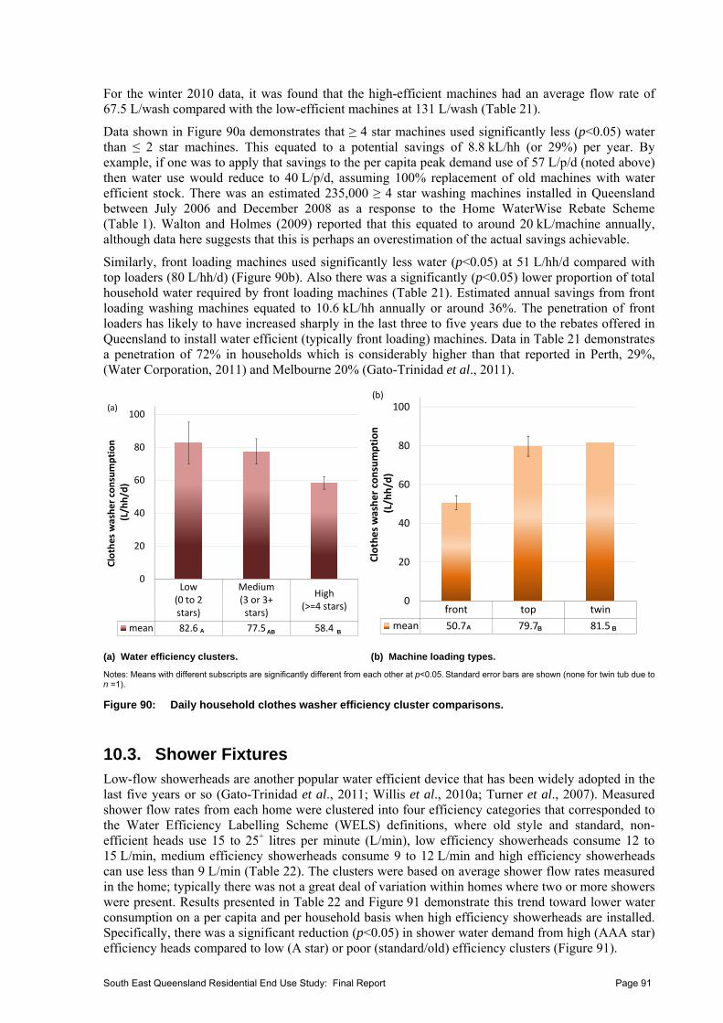
For the winter 2010 data, it was found that the high-efficient machines had an average flow rate of 67.5 L/wash compared with the low-efficient machines at 131 L/wash (Table 21).
Data shown in Figure 90a demonstrates that ≥ 4 star machines used significantly less (p<0.05) water than ≤ 2 star machines. This equated to a potential savings of 8.8 kL/hh (or 29%) per year. By example, if one was to apply that savings to the per capita peak demand use of 57 L/p/d (noted above) then water use would reduce to 40 L/p/d, assuming 100% replacement of old machines with water efficient stock. There was an estimated 235,000 ≥ 4 star washing machines installed in Queensland between July 2006 and December 2008 as a response to the Home WaterWise Rebate Scheme (Table 1). Walton and Holmes (2009) reported that this equated to around 20 kL/machine annually, although data here suggests that this is perhaps an overestimation of the actual savings achievable.
Similarly, front loading machines used significantly less water (p<0.05) at 51 L/hh/d compared with top loaders (80 L/hh/d) (Figure 90b). Also there was a significantly (p<0.05) lower proportion of total household water required by front loading machines (Table 21). Estimated annual savings from front loading washing machines equated to 10.6 kL/hh annually or around 36%. The penetration of front loaders has likely to have increased sharply in the last three to five years due to the rebates offered in Queensland to install water efficient (typically front loading) machines. Data in Table 21 demonstrates a penetration of 72% in households which is considerably higher than that reported in Perth, 29%, (Water Corporation, 2011) and Melbourne 20% (Gato-Trinidad et al., 2011).
Low(0 to 2stars)
Medium(3 or 3+stars)
High(>=4 stars)
mean 82.6 77.5 58.4
0
20
40
60
80
100
Clothes washer consumption
(L/hh/d)
A AB B
(a)
front top twin
mean 50.7 79.7 81.5
0
20
40
60
80
100
Clothes washer consumption
(L/hh/d)
A B B
(b)
(a) Water efficiency clusters. (b) Machine loading types.
Notes: Means with different subscripts are significantly different from each other at p<0.05. Standard error bars are shown (none for twin tub due to n =1).
Figure 90: Daily household clothes washer efficiency cluster comparisons.
10.3. Shower Fixtures Low-flow showerheads are another popular water efficient device that has been widely adopted in the last five years or so (Gato-Trinidad et al., 2011; Willis et al., 2010a; Turner et al., 2007). Measured shower flow rates from each home were clustered into four efficiency categories that corresponded to the Water Efficiency Labelling Scheme (WELS) definitions, where old style and standard, non-efficient heads use 15 to 25+ litres per minute (L/min), low efficiency showerheads consume 12 to 15 L/min, medium efficiency showerheads consume 9 to 12 L/min and high efficiency showerheads can use less than 9 L/min (Table 22). The clusters were based on average shower flow rates measured in the home; typically there was not a great deal of variation within homes where two or more showers were present. Results presented in Table 22 and Figure 91 demonstrate this trend toward lower water consumption on a per capita and per household basis when high efficiency showerheads are installed. Specifically, there was a significant reduction (p<0.05) in shower water demand from high (AAA star) efficiency heads compared to low (A star) or poor (standard/old) efficiency clusters (Figure 91).
South East Queensland Residential End Use Study: Final Report Page 91
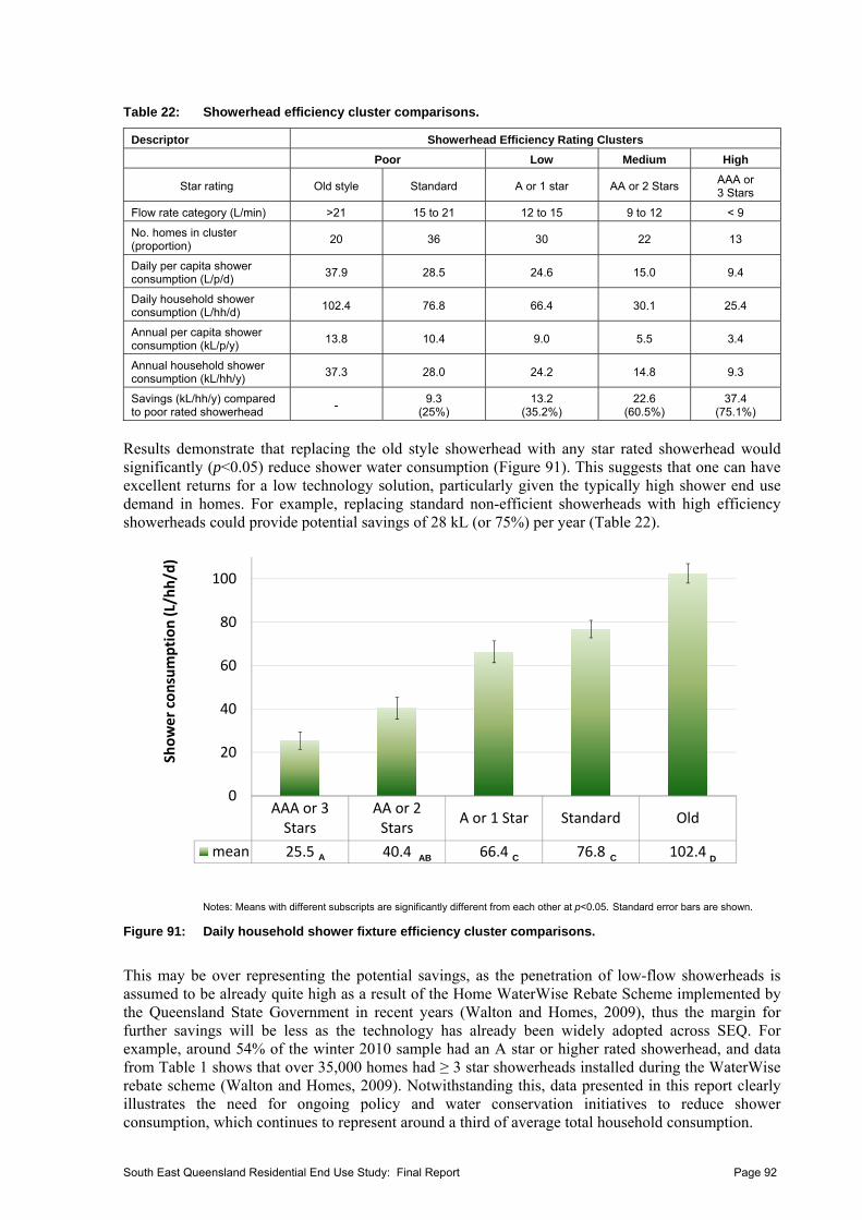
Table 22: Showerhead efficiency cluster comparisons.
Descriptor Showerhead Efficiency Rating Clusters
Poor Low Medium High
Star rating Old style Standard A or 1 star AA or 2 Stars AAA or 3 Stars
Flow rate category (L/min) >21 15 to 21 12 to 15 9 to 12 < 9
No. homes in cluster (proportion)
20 36 30 22 13
Daily per capita shower consumption (L/p/d)
37.9 28.5 24.6 15.0 9.4
Daily household shower consumption (L/hh/d)
102.4 76.8 66.4 30.1 25.4
Annual per capita shower consumption (kL/p/y)
13.8 10.4 9.0 5.5 3.4
Annual household shower consumption (kL/hh/y)
37.3 28.0 24.2 14.8 9.3
Savings (kL/hh/y) compared to poor rated showerhead
- 9.3
(25%) 13.2
(35.2%) 22.6
(60.5%) 37.4
(75.1%)
Results demonstrate that replacing the old style showerhead with any star rated showerhead would significantly (p<0.05) reduce shower water consumption (Figure 91). This suggests that one can have excellent returns for a low technology solution, particularly given the typically high shower end use demand in homes. For example, replacing standard non-efficient showerheads with high efficiency showerheads could provide potential savings of 28 kL (or 75%) per year (Table 22).
AAA or 3Stars
AA or 2Stars
A or 1 Star Standard Old
mean 25.5 40.4 66.4 76.8 102.4
0
20
40
60
80
100
Shower consumption (L/hh/d)
A AB C DC
Notes: Means with different subscripts are significantly different from each other at p<0.05. Standard error bars are shown.
Figure 91: Daily household shower fixture efficiency cluster comparisons.
This may be over representing the potential savings, as the penetration of low-flow showerheads is assumed to be already quite high as a result of the Home WaterWise Rebate Scheme implemented by the Queensland State Government in recent years (Walton and Homes, 2009), thus the margin for further savings will be less as the technology has already been widely adopted across SEQ. For example, around 54% of the winter 2010 sample had an A star or higher rated showerhead, and data from Table 1 shows that over 35,000 homes had ≥ 3 star showerheads installed during the WaterWise rebate scheme (Walton and Homes, 2009). Notwithstanding this, data presented in this report clearly illustrates the need for ongoing policy and water conservation initiatives to reduce shower consumption, which continues to represent around a third of average total household consumption.
South East Queensland Residential End Use Study: Final Report Page 92
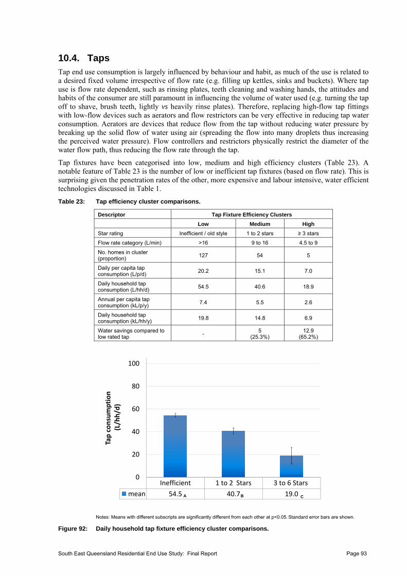
10.4. Taps Tap end use consumption is largely influenced by behaviour and habit, as much of the use is related to a desired fixed volume irrespective of flow rate (e.g. filling up kettles, sinks and buckets). Where tap use is flow rate dependent, such as rinsing plates, teeth cleaning and washing hands, the attitudes and habits of the consumer are still paramount in influencing the volume of water used (e.g. turning the tap off to shave, brush teeth, lightly vs heavily rinse plates). Therefore, replacing high-flow tap fittings with low-flow devices such as aerators and flow restrictors can be very effective in reducing tap water consumption. Aerators are devices that reduce flow from the tap without reducing water pressure by breaking up the solid flow of water using air (spreading the flow into many droplets thus increasing the perceived water pressure). Flow controllers and restrictors physically restrict the diameter of the water flow path, thus reducing the flow rate through the tap.
Tap fixtures have been categorised into low, medium and high efficiency clusters (Table 23). A notable feature of Table 23 is the number of low or inefficient tap fixtures (based on flow rate). This is surprising given the penetration rates of the other, more expensive and labour intensive, water efficient technologies discussed in Table 1.
Table 23: Tap efficiency cluster comparisons.
Descriptor Tap Fixture Efficiency Clusters
Low Medium High
Star rating Inefficient / old style 1 to 2 stars ≥ 3 stars
Flow rate category (L/min) >16 9 to 16 4.5 to 9
No. homes in cluster (proportion)
127 54 5
Daily per capita tap consumption (L/p/d)
20.2 15.1 7.0
Daily household tap consumption (L/hh/d)
54.5 40.6 18.9
Annual per capita tap consumption (kL/p/y)
7.4 5.5 2.6
Daily household tap consumption (kL/hh/y)
19.8 14.8 6.9
Water savings compared to low rated tap
- 5
(25.3%) 12.9
(65.2%)
Inefficient 1 to 2 Stars 3 to 6 Stars
mean 54.5 40.7 19.0
0
20
40
60
80
100
Tap consumption
(L/hh/d)
A B C
Notes: Means with different subscripts are significantly different from each other at p<0.05. Standard error bars are shown.
Figure 92: Daily household tap fixture efficiency cluster comparisons.
South East Queensland Residential End Use Study: Final Report Page 93
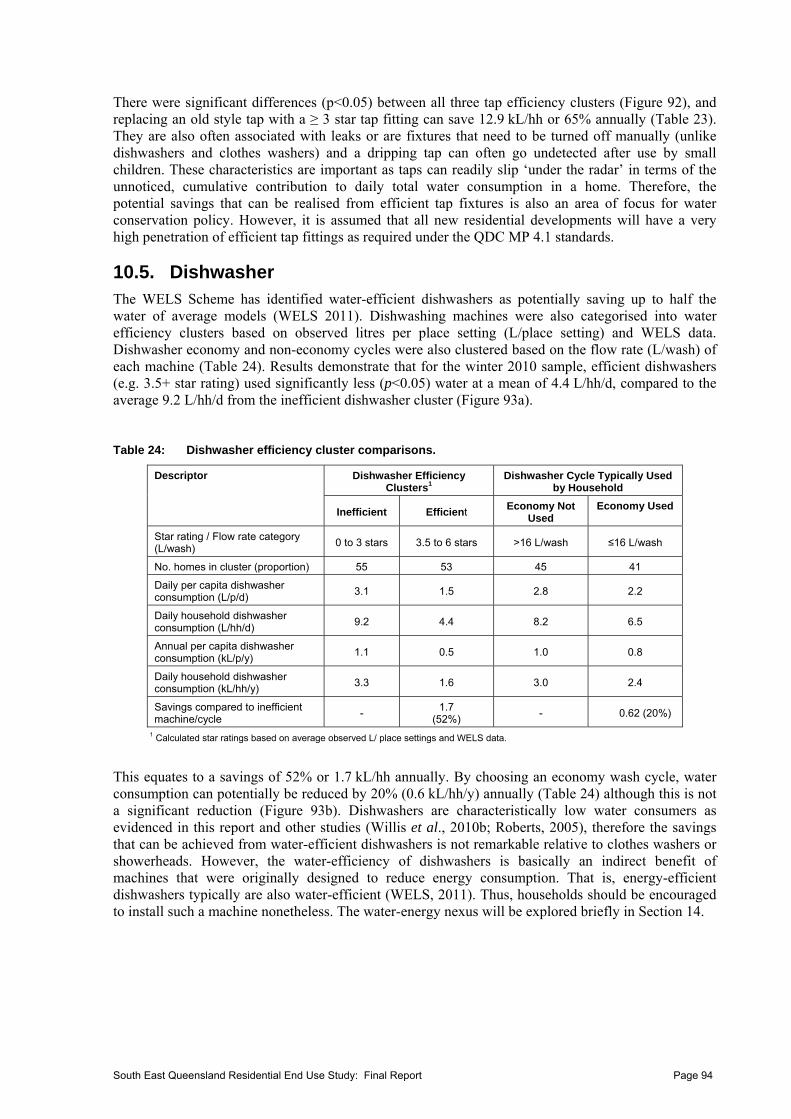
There were significant differences (p<0.05) between all three tap efficiency clusters (Figure 92), and replacing an old style tap with a ≥ 3 star tap fitting can save 12.9 kL/hh or 65% annually (Table 23). They are also often associated with leaks or are fixtures that need to be turned off manually (unlike dishwashers and clothes washers) and a dripping tap can often go undetected after use by small children. These characteristics are important as taps can readily slip ‘under the radar’ in terms of the unnoticed, cumulative contribution to daily total water consumption in a home. Therefore, the potential savings that can be realised from efficient tap fixtures is also an area of focus for water conservation policy. However, it is assumed that all new residential developments will have a very high penetration of efficient tap fittings as required under the QDC MP 4.1 standards.
10.5. Dishwasher The WELS Scheme has identified water-efficient dishwashers as potentially saving up to half the water of average models (WELS 2011). Dishwashing machines were also categorised into water efficiency clusters based on observed litres per place setting (L/place setting) and WELS data. Dishwasher economy and non-economy cycles were also clustered based on the flow rate (L/wash) of each machine (Table 24). Results demonstrate that for the winter 2010 sample, efficient dishwashers (e.g. 3.5+ star rating) used significantly less (p<0.05) water at a mean of 4.4 L/hh/d, compared to the average 9.2 L/hh/d from the inefficient dishwasher cluster (Figure 93a).
Table 24: Dishwasher efficiency cluster comparisons.
Dishwasher Efficiency Clusters1
Dishwasher Cycle Typically Used by Household
Descriptor
Inefficient Efficient Economy Not
Used Economy Used
Star rating / Flow rate category (L/wash)
0 to 3 stars 3.5 to 6 stars >16 L/wash ≤16 L/wash
No. homes in cluster (proportion) 55 53 45 41
Daily per capita dishwasher consumption (L/p/d)
3.1 1.5 2.8 2.2
Daily household dishwasher consumption (L/hh/d)
9.2 4.4 8.2 6.5
Annual per capita dishwasher consumption (kL/p/y)
1.1 0.5 1.0 0.8
Daily household dishwasher consumption (kL/hh/y)
3.3 1.6 3.0 2.4
Savings compared to inefficient machine/cycle
- 1.7
(52%) - 0.62 (20%)
1 Calculated star ratings based on average observed L/ place settings and WELS data.
This equates to a savings of 52% or 1.7 kL/hh annually. By choosing an economy wash cycle, water consumption can potentially be reduced by 20% (0.6 kL/hh/y) annually (Table 24) although this is not a significant reduction (Figure 93b). Dishwashers are characteristically low water consumers as evidenced in this report and other studies (Willis et al., 2010b; Roberts, 2005), therefore the savings that can be achieved from water-efficient dishwashers is not remarkable relative to clothes washers or showerheads. However, the water-efficiency of dishwashers is basically an indirect benefit of machines that were originally designed to reduce energy consumption. That is, energy-efficient dishwashers typically are also water-efficient (WELS, 2011). Thus, households should be encouraged to install such a machine nonetheless. The water-energy nexus will be explored briefly in Section 14.
South East Queensland Residential End Use Study: Final Report Page 94
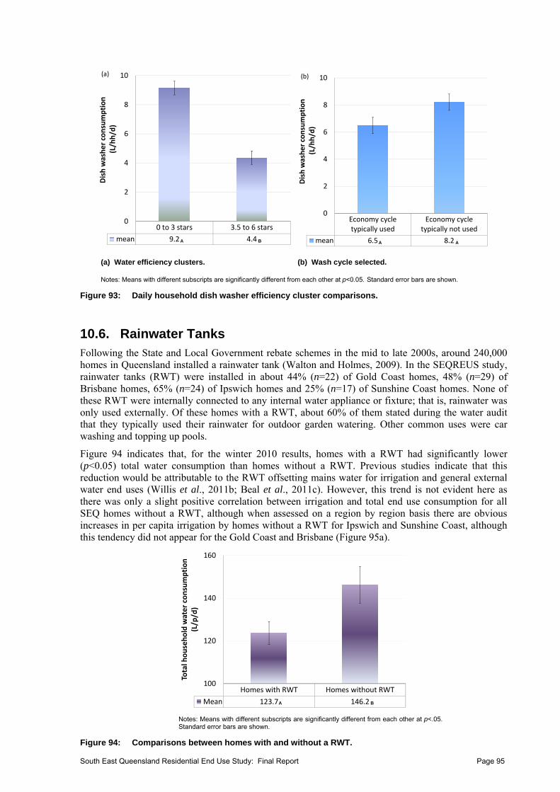
0 to 3 stars 3.5 to 6 stars
mean 9.2 4.4
0
2
4
6
8
10
Dish washer consumption
(L/hh/d)
A B
(a)
Economy cycletypically used
Economy cycletypically not used
mean 6.5 8.2
0
2
4
6
8
10
Dish washer consumption
(L/hh/d)
A A
(b)
(a) Water efficiency clusters. (b) Wash cycle selected.
Notes: Means with different subscripts are significantly different from each other at p<0.05. Standard error bars are shown.
Figure 93: Daily household dish washer efficiency cluster comparisons.
10.6. Rainwater Tanks Following the State and Local Government rebate schemes in the mid to late 2000s, around 240,000 homes in Queensland installed a rainwater tank (Walton and Holmes, 2009). In the SEQREUS study, rainwater tanks (RWT) were installed in about 44% (n=22) of Gold Coast homes, 48% (n=29) of Brisbane homes, 65% (n=24) of Ipswich homes and 25% (n=17) of Sunshine Coast homes. None of these RWT were internally connected to any internal water appliance or fixture; that is, rainwater was only used externally. Of these homes with a RWT, about 60% of them stated during the water audit that they typically used their rainwater for outdoor garden watering. Other common uses were car washing and topping up pools.
Figure 94 indicates that, for the winter 2010 results, homes with a RWT had significantly lower (p<0.05) total water consumption than homes without a RWT. Previous studies indicate that this reduction would be attributable to the RWT offsetting mains water for irrigation and general external water end uses (Willis et al., 2011b; Beal et al., 2011c). However, this trend is not evident here as there was only a slight positive correlation between irrigation and total end use consumption for all SEQ homes without a RWT, although when assessed on a region by region basis there are obvious increases in per capita irrigation by homes without a RWT for Ipswich and Sunshine Coast, although this tendency did not appear for the Gold Coast and Brisbane (Figure 95a).
Homes with RWT Homes without RWT
Mean 123.7 146.2
100
120
140
160
Total household water consumption
(L/p/d)
A B Notes: Means with different subscripts are significantly different from each other at p<.05.
Standard error bars are shown.
Figure 94: Comparisons between homes with and without a RWT.
South East Queensland Residential End Use Study: Final Report Page 95
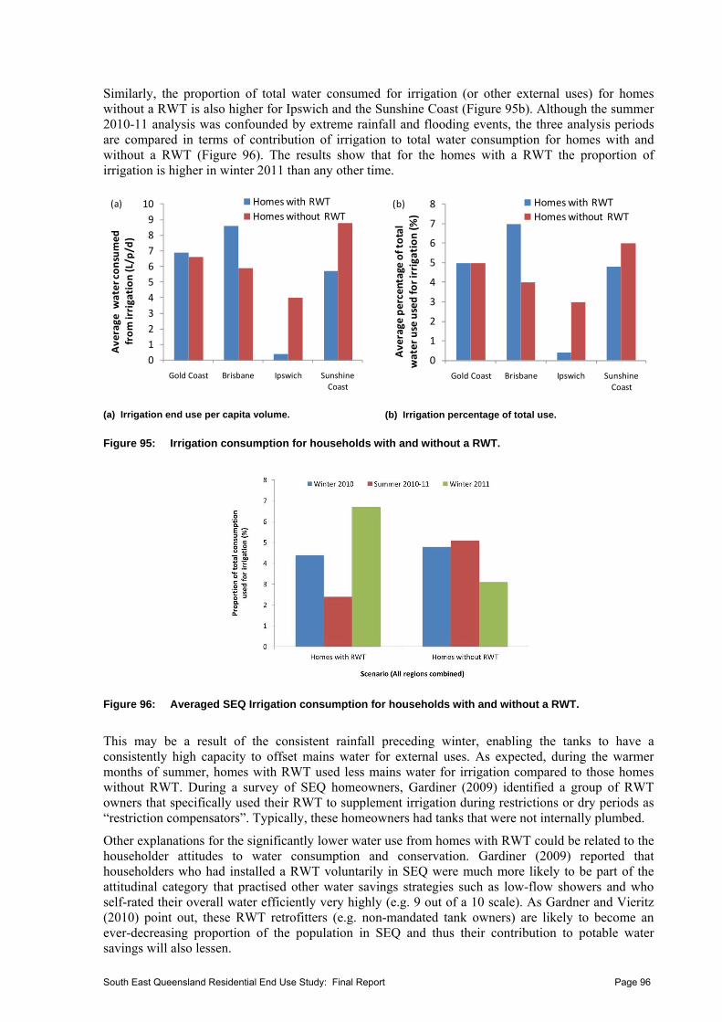
Similarly, the proportion of total water consumed for irrigation (or other external uses) for homes without a RWT is also higher for Ipswich and the Sunshine Coast (Figure 95b). Although the summer 2010-11 analysis was confounded by extreme rainfall and flooding events, the three analysis periods are compared in terms of contribution of irrigation to total water consumption for homes with and without a RWT (Figure 96). The results show that for the homes with a RWT the proportion of irrigation is higher in winter 2011 than any other time.
0
1
2
3
4
5
6
7
8
9
10
Gold Coast Brisbane Ipswich Sunshine Coast
Average w
ater consumed
from irrigation (L/p/d)
Homes with RWT
Homes without RWT(a)
(a) Irrigation end use per capita volume.
0
1
2
3
4
5
6
7
8
Gold Coast Brisbane Ipswich Sunshine Coast
Average
percentage of total
water use used for irrigation (%)
Homes with RWT
Homes without RWT(b)
(b) Irrigation percentage of total use.
Figure 95: Irrigation consumption for households with and without a RWT.
Figure 96: Averaged SEQ Irrigation consumption for households with and without a RWT.
This may be a result of the consistent rainfall preceding winter, enabling the tanks to have a consistently high capacity to offset mains water for external uses. As expected, during the warmer months of summer, homes with RWT used less mains water for irrigation compared to those homes without RWT. During a survey of SEQ homeowners, Gardiner (2009) identified a group of RWT owners that specifically used their RWT to supplement irrigation during restrictions or dry periods as “restriction compensators”. Typically, these homeowners had tanks that were not internally plumbed.
Other explanations for the significantly lower water use from homes with RWT could be related to the householder attitudes to water consumption and conservation. Gardiner (2009) reported that householders who had installed a RWT voluntarily in SEQ were much more likely to be part of the attitudinal category that practised other water savings strategies such as low-flow showers and who self-rated their overall water efficiently very highly (e.g. 9 out of a 10 scale). As Gardner and Vieritz (2010) point out, these RWT retrofitters (e.g. non-mandated tank owners) are likely to become an ever-decreasing proportion of the population in SEQ and thus their contribution to potable water savings will also lessen.
South East Queensland Residential End Use Study: Final Report Page 96
11. STOCK EFFICIENCY INFLUENCE ON PEAK DEMAND
11.1. Introduction The above sections have clearly shown how water-efficient stock can significantly reduce total household water consumption. This section will now briefly explore how water-efficient stock can reduce the average day peak hour demand by examining diurnal patterns from homes with and without water-efficient technology. The end uses which drive these reductions in peak demand will be identified. The relevance of this research relates to future infrastructure and network distribution modelling which use peaking factors for designing the diameters of the distribution pipes. Optimisation and deferral of water supply infrastructure by using current and representative peak demand data is likely to be of significant interest to water utilities. Moreover, also considering reductions in peak demand that will result from demand management interventions, when conducting least-cost water planning assessments, will further enhance the attractiveness of such options.
11.2. Overview of Methods Household stock efficiency information was obtained from household water audits with efficiency ratings recorded as per the WELS star rating system. The efficiency information included flow rates of showerheads, average flow rates of indoor taps, and the volume of toilet cisterns, in order to establish water used per flush, star rating and water used per cycle of washing machines and dishwashers. In an attempt to develop a representative composite star rating, reflecting the combined efficiency of the entire household water appliance/fixture stock composition, a weighted classification system was designed and implemented. The overall household efficiency weighting system takes account of both the contribution of each end use to total consumption and the star rating of the various indoor fixtures/appliances within each household. Although a dishwasher could be allocated a WELS rating, it is such a small component (i.e. < 2%) of overall household water use it is unlikely to discernibly affect peak flows and was therefore not included in the composite household star rating. The four primary end uses accounted for over 87.5% of the total water use within the sample and therefore would be the significant contributors to average day (AD) peak hour diurnal flows. After each home’s overall efficiency was calculated, a frequency distribution was created in order to classify the range of household composite star rating categories and identify potential efficiency clusters (Figure 97).
0
1
2
3
4
5
Overall Star Rating
Household ID
Toilet Shower Tap Clothes Washer
(a)
0
0.25
0.5
0.75
1
0
0.02
0.04
0.06
0.08
0.1
0.12
1.1 1.4 1.7 2 2.3 2.6 2.9 3.2 3.5 3.8 4.1 4.4
Cumulative frequency distribution
Relative frequency distribution
Total weighted efficiency rating
Relative Frequency
Cumulative Frequency
(b)
(a) Weighted star rating distribution. (b) Total frequency and cumulative distribution.
Figure 97: Household efficiency frequency and cumulative distributions.
South East Queensland Residential End Use Study: Final Report Page 97
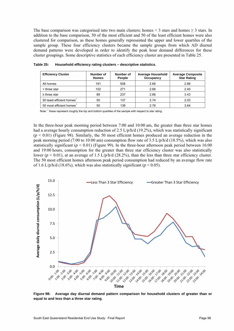
The base comparison was categorised into two main clusters; homes < 3 stars and homes ≥ 3 stars. In addition to the base comparison, 50 of the most efficient and 50 of the least efficient homes were also clustered for comparison, as these homes generally represented the upper and lower quartiles of the sample group. These four efficiency clusters became the sample groups from which AD diurnal demand patterns were developed in order to identify the peak hour demand differences for these cluster groupings. Some descriptive statistics of each efficiency cluster are presented in Table 25. Table 25: Household efficiency rating clusters – descriptive statistics.
Efficiency Cluster Number of Homes
Number of People
Average Household Occupancy
Average Composite Star Rating
All homes 191 508 2.66 2.88
< three star 102 271 2.66 2.40
≥ three star 89 237 2.66 3.43
50 least efficient homes1 50 137 2.74 2.03
50 most efficient homes1 50 138 2.76 3.64
Note: 1 these represent roughly the top and bottom quartiles of the sample with respect to star rating.
In the three-hour peak morning period between 7:00 and 10:00 am, the greater than three star homes had a average hourly consumption reduction of 2.5 L/p/h/d (19.2%), which was statistically significant (p < 0.01) (Figure 98). Similarly, the 50 most efficient homes produced an average reduction in the peak morning period (7:00 to 10:00 am) consumption flow rate of 3.5 L/p/h/d (18.5%), which was also statistically significant (p < 0.01) (Figure 99). In the three-hour afternoon peak period between 16:00 and 19:00 hours, consumption for the greater than three star efficiency cluster was also statistically lower (p < 0.01), at an average of 1.5 L/p/h/d (28.2%), than the less than three star efficiency cluster. The 50 most efficient homes afternoon peak period consumption had reduced by an average flow rate of 1.6 L/p/h/d (18.6%), which was also statistically significant (p < 0.05).
0.0
2.5
5.0
7.5
10.0
12.5
15.0
Average daily diurnal consumption (L/p/h/d)
Time
Less Than 3 Star Efficiency Greater Than 3 Star Efficiency
Figure 98: Average day diurnal demand pattern comparison for household clusters of greater than or equal to and less than a three star rating.
South East Queensland Residential End Use Study: Final Report Page 98
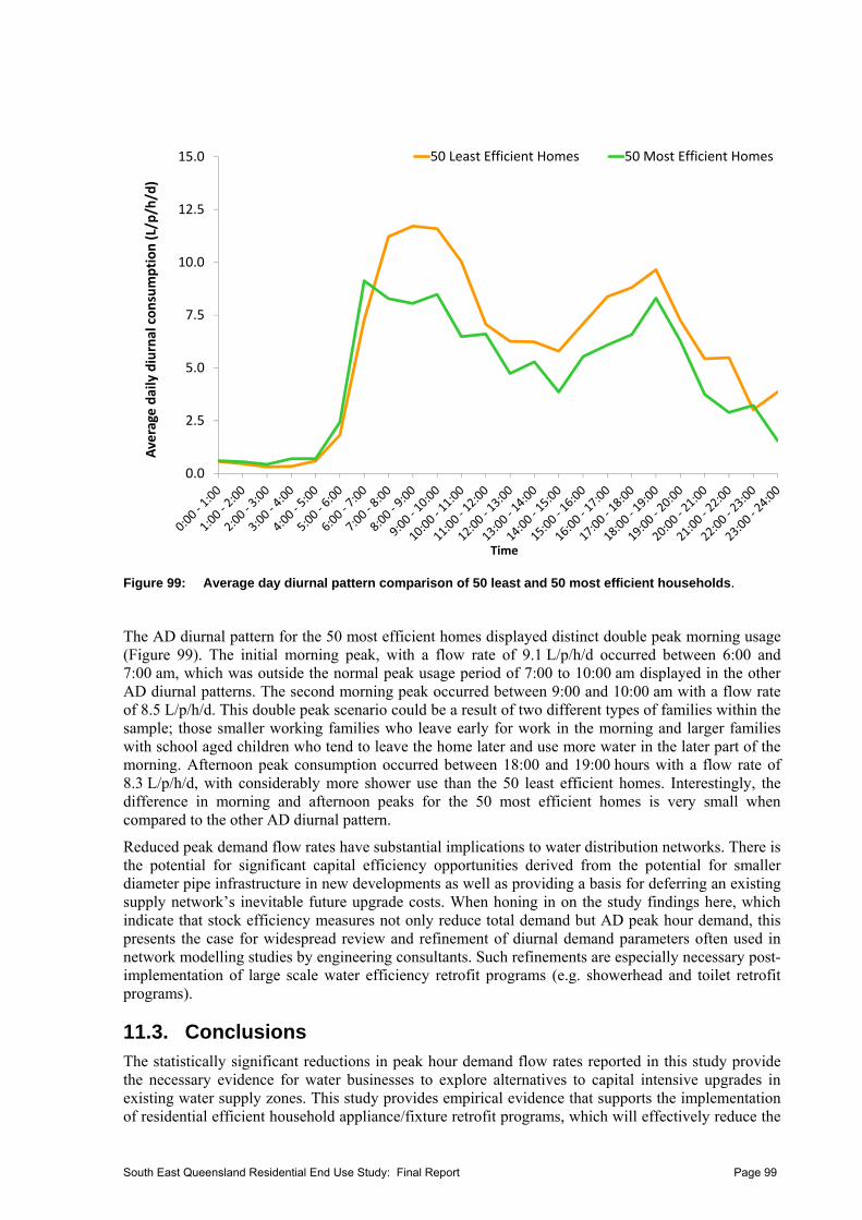
0.0
2.5
5.0
7.5
10.0
12.5
15.0Average daily diurnal consumption (L/p/h/d)
Time
50 Least Efficient Homes 50 Most Efficient Homes
Figure 99: Average day diurnal pattern comparison of 50 least and 50 most efficient households.
The AD diurnal pattern for the 50 most efficient homes displayed distinct double peak morning usage (Figure 99). The initial morning peak, with a flow rate of 9.1 L/p/h/d occurred between 6:00 and 7:00 am, which was outside the normal peak usage period of 7:00 to 10:00 am displayed in the other AD diurnal patterns. The second morning peak occurred between 9:00 and 10:00 am with a flow rate of 8.5 L/p/h/d. This double peak scenario could be a result of two different types of families within the sample; those smaller working families who leave early for work in the morning and larger families with school aged children who tend to leave the home later and use more water in the later part of the morning. Afternoon peak consumption occurred between 18:00 and 19:00 hours with a flow rate of 8.3 L/p/h/d, with considerably more shower use than the 50 least efficient homes. Interestingly, the difference in morning and afternoon peaks for the 50 most efficient homes is very small when compared to the other AD diurnal pattern.
Reduced peak demand flow rates have substantial implications to water distribution networks. There is the potential for significant capital efficiency opportunities derived from the potential for smaller diameter pipe infrastructure in new developments as well as providing a basis for deferring an existing supply network’s inevitable future upgrade costs. When honing in on the study findings here, which indicate that stock efficiency measures not only reduce total demand but AD peak hour demand, this presents the case for widespread review and refinement of diurnal demand parameters often used in network modelling studies by engineering consultants. Such refinements are especially necessary post-implementation of large scale water efficiency retrofit programs (e.g. showerhead and toilet retrofit programs).
11.3. Conclusions The statistically significant reductions in peak hour demand flow rates reported in this study provide the necessary evidence for water businesses to explore alternatives to capital intensive upgrades in existing water supply zones. This study provides empirical evidence that supports the implementation of residential efficient household appliance/fixture retrofit programs, which will effectively reduce the
South East Queensland Residential End Use Study: Final Report Page 99
South East Queensland Residential End Use Study: Final Report Page 100
critical peak demand values used in network modelling design, and defer urgent water service infrastructure upgrade requirements. This suggests excellent capital efficiency opportunities for water supply infrastructure, specifically through the deferral of future upgrade costs in existing areas, and the potential decrease in sizing for new network distribution elements in growing population areas. As a result of the likelihood of considerably lower peak flows in future developments, particularly where development codes mandate the installation of water efficient technology, it is recommended that future network modelling tasks completed by engineers incorporate real reductions in future demand flow rates as well as reduced network peaking factors as a result of water efficient technology.
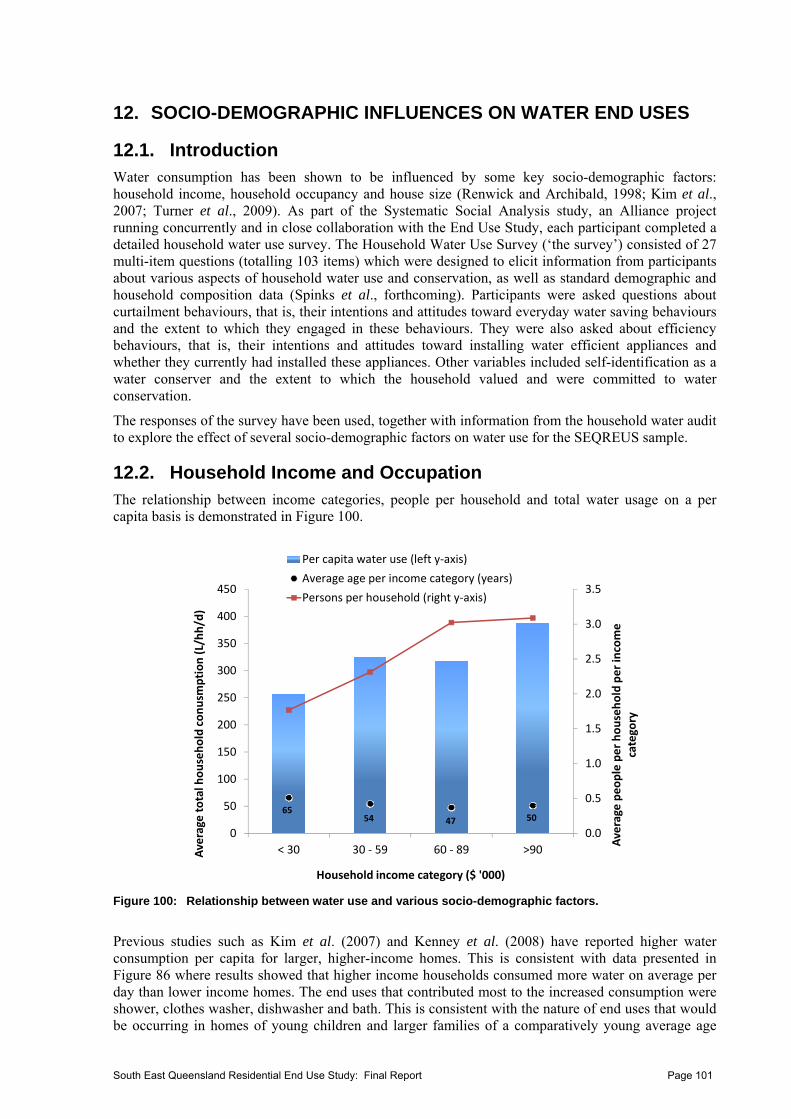
12. SOCIO-DEMOGRAPHIC INFLUENCES ON WATER END USES
12.1. Introduction Water consumption has been shown to be influenced by some key socio-demographic factors: household income, household occupancy and house size (Renwick and Archibald, 1998; Kim et al., 2007; Turner et al., 2009). As part of the Systematic Social Analysis study, an Alliance project running concurrently and in close collaboration with the End Use Study, each participant completed a detailed household water use survey. The Household Water Use Survey (‘the survey’) consisted of 27 multi-item questions (totalling 103 items) which were designed to elicit information from participants about various aspects of household water use and conservation, as well as standard demographic and household composition data (Spinks et al., forthcoming). Participants were asked questions about curtailment behaviours, that is, their intentions and attitudes toward everyday water saving behaviours and the extent to which they engaged in these behaviours. They were also asked about efficiency behaviours, that is, their intentions and attitudes toward installing water efficient appliances and whether they currently had installed these appliances. Other variables included self-identification as a water conserver and the extent to which the household valued and were committed to water conservation.
The responses of the survey have been used, together with information from the household water audit to explore the effect of several socio-demographic factors on water use for the SEQREUS sample.
12.2. Household Income and Occupation The relationship between income categories, people per household and total water usage on a per capita basis is demonstrated in Figure 100.
0.0
0.5
1.0
1.5
2.0
2.5
3.0
3.5
0
50
100
150
200
250
300
350
400
450
< 30 30 ‐ 59 60 ‐ 89 >90
Average people per household per income
category
Average total household conusm
ption (L/hh/d)
Household income category ($ '000)
Per capita water use (left y‐axis)
Average age per income category (years)
Persons per household (right y‐axis)
65504754
Figure 100: Relationship between water use and various socio-demographic factors.
Previous studies such as Kim et al. (2007) and Kenney et al. (2008) have reported higher water consumption per capita for larger, higher-income homes. This is consistent with data presented in Figure 86 where results showed that higher income households consumed more water on average per day than lower income homes. The end uses that contributed most to the increased consumption were shower, clothes washer, dishwasher and bath. This is consistent with the nature of end uses that would be occurring in homes of young children and larger families of a comparatively young average age
South East Queensland Residential End Use Study: Final Report Page 101
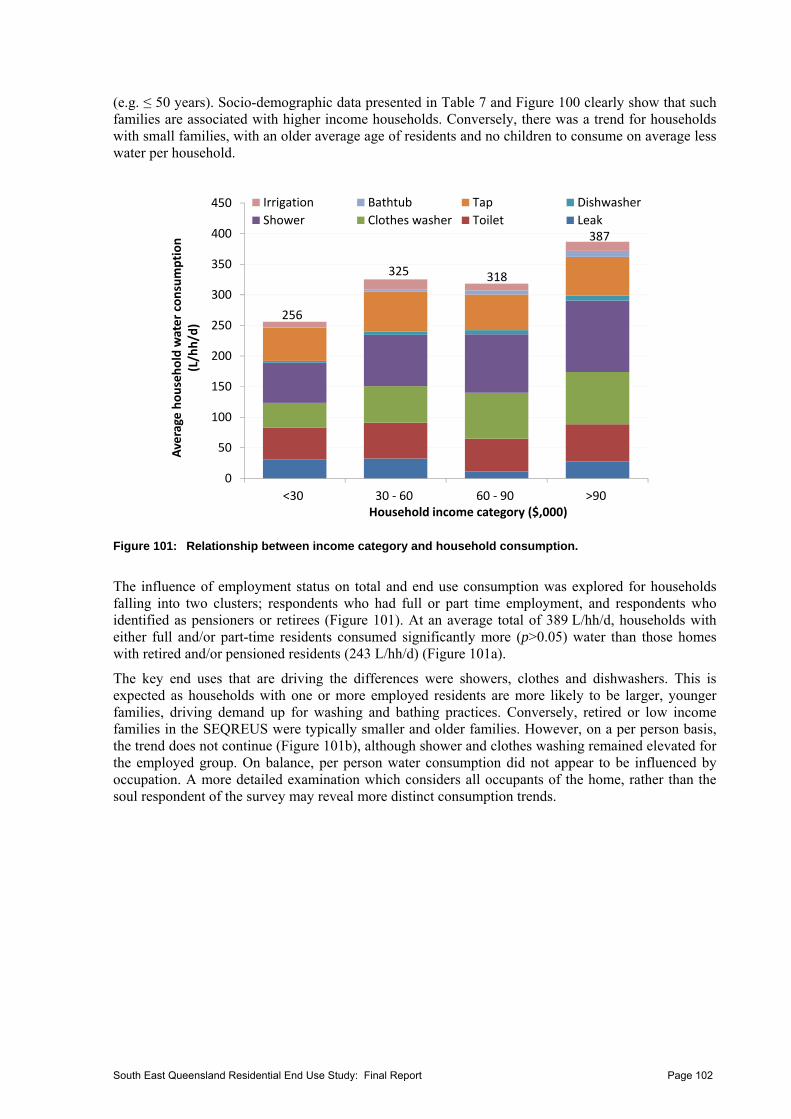
(e.g. ≤ 50 years). Socio-demographic data presented in Table 7 and Figure 100 clearly show that such families are associated with higher income households. Conversely, there was a trend for households with small families, with an older average age of residents and no children to consume on average less water per household.
0
50
100
150
200
250
300
350
400
450
<30 30 ‐ 60 60 ‐ 90 >90
Average household water consumption
(L/hh/d)
Household income category ($,000)
Irrigation Bathtub Tap Dishwasher
Shower Clothes washer Toilet Leak
325 318
387
256
Figure 101: Relationship between income category and household consumption.
The influence of employment status on total and end use consumption was explored for households falling into two clusters; respondents who had full or part time employment, and respondents who identified as pensioners or retirees (Figure 101). At an average total of 389 L/hh/d, households with either full and/or part-time residents consumed significantly more (p>0.05) water than those homes with retired and/or pensioned residents (243 L/hh/d) (Figure 101a).
The key end uses that are driving the differences were showers, clothes and dishwashers. This is expected as households with one or more employed residents are more likely to be larger, younger families, driving demand up for washing and bathing practices. Conversely, retired or low income families in the SEQREUS were typically smaller and older families. However, on a per person basis, the trend does not continue (Figure 101b), although shower and clothes washing remained elevated for the employed group. On balance, per person water consumption did not appear to be influenced by occupation. A more detailed examination which considers all occupants of the home, rather than the soul respondent of the survey may reveal more distinct consumption trends.
South East Queensland Residential End Use Study: Final Report Page 102
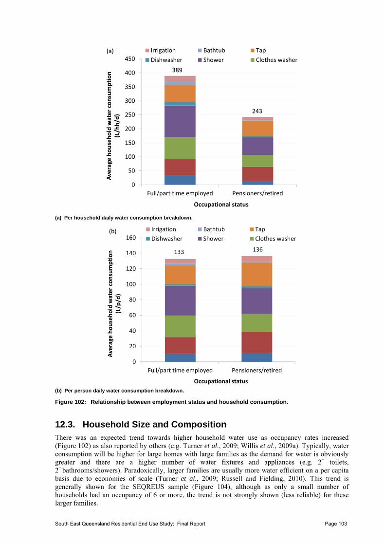
0
50
100
150
200
250
300
350
400
450
Full/part time employed Pensioners/retired
Average household water consumption
(L/hh/d)
Occupational status
Irrigation Bathtub Tap
Dishwasher Shower Clothes washer
243
389
(a)
(a) Per household daily water consumption breakdown.
0
20
40
60
80
100
120
140
160
Full/part time employed Pensioners/retired
Average household water consumption
(L/p/d)
Occupational status
Irrigation Bathtub Tap
Dishwasher Shower Clothes washer
136133
(b)
(b) Per person daily water consumption breakdown.
Figure 102: Relationship between employment status and household consumption.
12.3. Household Size and Composition There was an expected trend towards higher household water use as occupancy rates increased (Figure 102) as also reported by others (e.g. Turner et al., 2009; Willis et al., 2009a). Typically, water consumption will be higher for large homes with large families as the demand for water is obviously greater and there are a higher number of water fixtures and appliances (e.g. 2+ toilets, 2+ bathrooms/showers). Paradoxically, larger families are usually more water efficient on a per capita basis due to economies of scale (Turner et al., 2009; Russell and Fielding, 2010). This trend is generally shown for the SEQREUS sample (Figure 104), although as only a small number of households had an occupancy of 6 or more, the trend is not strongly shown (less reliable) for these larger families.
South East Queensland Residential End Use Study: Final Report Page 103
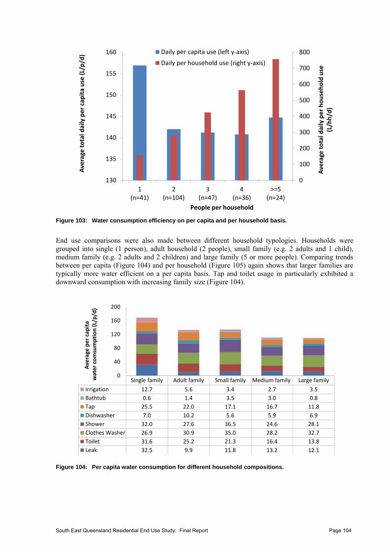
0
100
200
300
400
500
600
700
800
130
135
140
145
150
155
160
1(n=41)
2(n=104)
3(n=47)
4(n=36)
>=5(n=24)
Average total daily per household use
(L/hh/d)
Average total daily per capita use (L/p/d)
People per household
Daily per capita use (left y‐axis)
Daily per household use (right y‐axis)
Figure 103: Water consumption efficiency on per capita and per household basis.
End use comparisons were also made between different household typologies. Households were grouped into single (1 person), adult household (2 people), small family (e.g. 2 adults and 1 child), medium family (e.g. 2 adults and 2 children) and large family (5 or more people). Comparing trends between per capita (Figure 104) and per household (Figure 105) again shows that larger families are typically more water efficient on a per capita basis. Tap and toilet usage in particularly exhibited a downward consumption with increasing family size (Figure 104).
Single family Adult family Small family Medium family Large family
Irrigation 12.7 5.6 3.4 2.7 3.5
Bathtub 0.6 1.4 3.5 3.0 0.8
Tap 25.5 22.0 17.1 16.7 11.8
Dishwasher 7.0 10.2 5.6 5.9 6.9
Shower 32.0 27.6 36.5 24.6 28.1
Clothes Washer 26.9 30.9 35.0 28.2 32.7
Toilet 31.6 25.2 21.3 16.4 13.8
Leak 32.5 9.9 11.8 13.2 12.1
0
40
80
120
160
200
Average per capita
water comsumption (L/p/d)
Figure 104: Per capita water consumption for different household compositions.
South East Queensland Residential End Use Study: Final Report Page 104
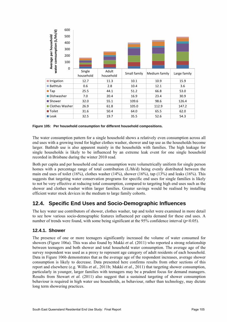
Singlehousehold
Adulthousehold
Small family Medium family Large family
Irrigation 12.7 11.3 10.1 10.9 15.9
Bathtub 0.6 2.8 10.4 12.1 3.6
Tap 25.5 44.1 51.2 66.8 53.0
Dishwasher 7.0 20.4 16.9 23.4 30.9
Shower 32.0 55.1 109.6 98.6 126.4
Clothes Washer 26.9 61.8 105.0 112.9 147.2
Toilet 31.6 50.4 64.0 65.5 62.0
Leak 32.5 19.7 35.5 52.6 54.3
0
100
200
300
400
500
600
Average per household
water comsumption (L/hh/d)
Figure 105: Per household consumption for different household compositions.
The water consumption pattern for a single household shows a relatively even consumption across all end uses with a growing trend for higher clothes washer, shower and tap use as the households become larger. Bathtub use is also apparent mainly in the households with families. The high leakage for single households is likely to be influenced by an extreme leak event for one single household recorded in Brisbane during the winter 2010 read.
Both per capita and per household end use consumption were volumetrically uniform for single person homes with a percentage range of total contribution (L/hh/d) being evenly distributed between the main end uses of toilet (16%), clothes washer (14%), shower (16%), tap (13%) and leaks (16%). This suggests that targeting water conservation programs for specific end uses for single families is likely to not be very effective at reducing total consumption, compared to targeting high end uses such as the shower and clothes washer within larger families. Greater savings would be realised by installing efficient water stock devices in the medium to large family cohorts.
12.4. Specific End Uses and Socio-Demographic Influences The key water use contributors of shower, clothes washer, tap and toilet were examined in more detail to see how various socio-demographic features influenced per capita demand for these end uses. A number of trends were found, with some being significant at the 95% confidence interval (p<0.05).
12.4.1. Shower
The presence of one or more teenagers significantly increased the volume of water consumed for showers (Figure 106a). This was also found by Makki et al. (2011) who reported a strong relationship between teenagers and both shower and total household water consumption. The average age of the survey respondent was used as a proxy to represent age category of adult residents of each household. Data in Figure 106b demonstrates that as the average age of the respondent increases, average shower consumption is likely to decrease. Data presented here confirms results from other sections of this report and elsewhere (e.g. Willis et al., 2011b; Makki et al., 2011) that targeting shower consumption, particularly in younger, larger families with teenagers may be a prudent focus for demand managers. Results from Stewart et al. (2011) also suggest that a sustained targeting of shower consumption behaviour is required in high water use households, as behaviour, rather than technology, may dictate long term showering practices.
South East Queensland Residential End Use Study: Final Report Page 105
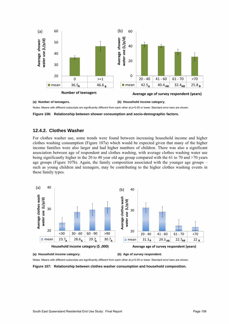
0 >=1
mean 36.5 46.6
20
30
40
50
60
Average shower
water use (L/p/d)
Number of teenagers
A B
(a)
20 ‐ 40 41 ‐ 60 61 ‐ 70 >70
mean 42.5 40.4 32.4 25.8
0
20
40
60
Average shower
water use (L/p/d)
Average age of survey respondent (years)
A AB
(b)
AB B
(a) Number of teenagers. (b) Household income category.
Notes: Means with different subscripts are significantly different from each other at p<0.05 or lower. Standard error bars are shown.
Figure 106: Relationship between shower consumption and socio-demographic factors.
12.4.2. Clothes Washer
For clothes washer use, some trends were found between increasing household income and higher clothes washing consumption (Figure 107a) which would be expected given that many of the higher income families were also larger and had higher numbers of children. There was also a significant association between age of respondent and clothes washing, with average clothes washing water use being significantly higher in the 20 to 40 year old age group compared with the 61 to 70 and >70 years age groups (Figure 107b). Again, the family composition associated with the younger age groups – such as young children and teenagers, may be contributing to the higher clothes washing events in these family types.
<30 30 ‐ 60 60 ‐ 90 >90
mean 23.7 28.6 29.7 30.7
20
30
40
Average
clothes wash
water use (L/p/d)
Household income category ($ ,000)
A A
(a)
A A
20 ‐ 40 41 ‐ 60 61 ‐ 70 >70
mean 31.3 29.3 22.7 22
20
30
40
Average clothes wash
water use (L/p/d)
Average age of survey respondent (years)
A AB
(b)
AB B
(a) Household income category. (b) Age of survey respondent.
Notes: Means with different subscripts are significantly different from each other at p<0.05 or lower. Standard error bars are shown.
Figure 107: Relationship between clothes washer consumption and household composition.
South East Queensland Residential End Use Study: Final Report Page 106
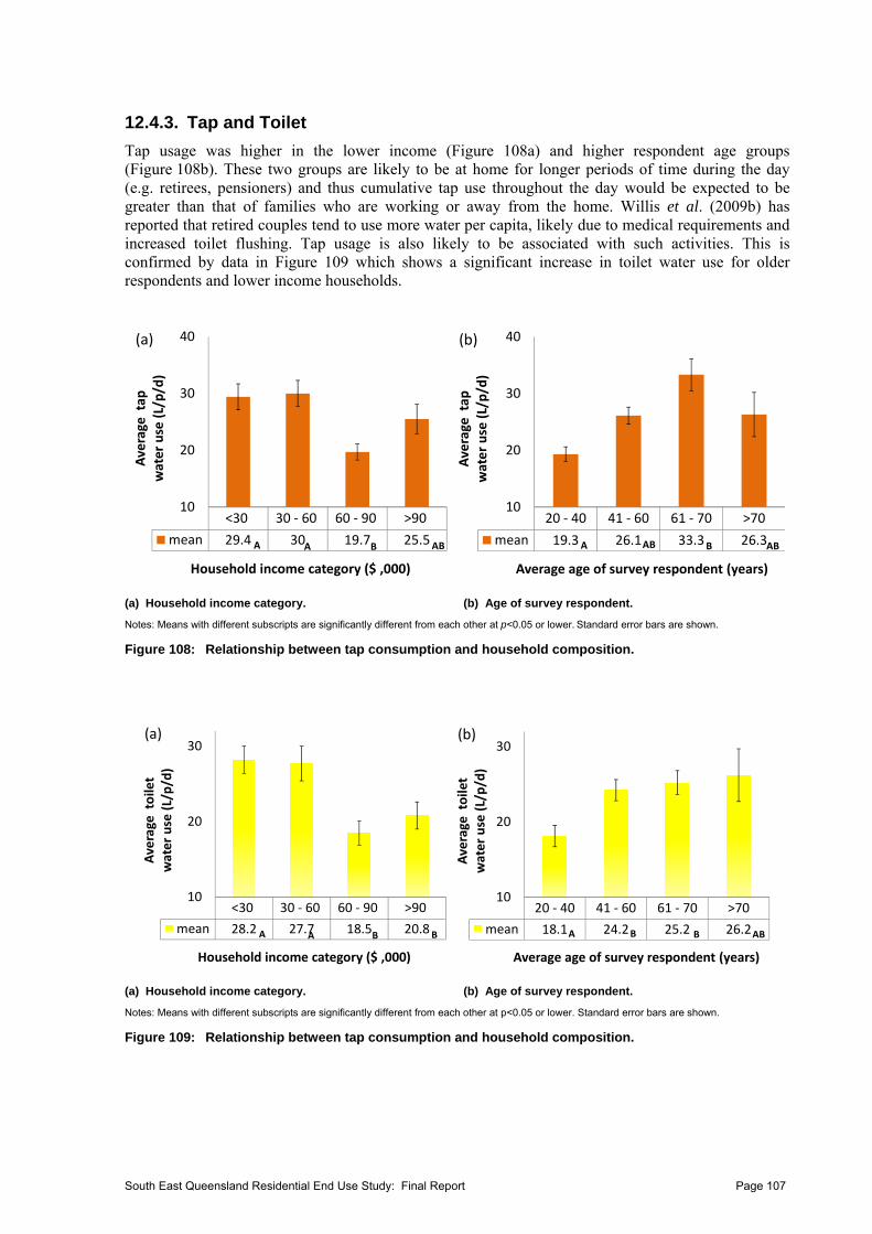
12.4.3. Tap and Toilet
Tap usage was higher in the lower income (Figure 108a) and higher respondent age groups (Figure 108b). These two groups are likely to be at home for longer periods of time during the day (e.g. retirees, pensioners) and thus cumulative tap use throughout the day would be expected to be greater than that of families who are working or away from the home. Willis et al. (2009b) has reported that retired couples tend to use more water per capita, likely due to medical requirements and increased toilet flushing. Tap usage is also likely to be associated with such activities. This is confirmed by data in Figure 109 which shows a significant increase in toilet water use for older respondents and lower income households.
<30 30 ‐ 60 60 ‐ 90 >90
mean 29.4 30 19.7 25.5
10
20
30
40
Average tap
water use (L/p/d)
Household income category ($ ,000)
A B
(a)
ABA
20 ‐ 40 41 ‐ 60 61 ‐ 70 >70
mean 19.3 26.1 33.3 26.3
10
20
30
40
Average tap
water use (L/p/d)
Average age of survey respondent (years)
A B
(b)
ABAB
(a) Household income category. (b) Age of survey respondent.
Notes: Means with different subscripts are significantly different from each other at p<0.05 or lower. Standard error bars are shown.
Figure 108: Relationship between tap consumption and household composition.
<30 30 ‐ 60 60 ‐ 90 >90
mean 28.2 27.7 18.5 20.8
10
20
30
Average toilet
water use (L/p/d)
Household income category ($ ,000)
A B
(a)
BA
20 ‐ 40 41 ‐ 60 61 ‐ 70 >70
mean 18.1 24.2 25.2 26.2
10
20
30
Average toilet
water use (L/p/d)
Average age of survey respondent (years)
A B
(b)
ABB
(a) Household income category. (b) Age of survey respondent.
Notes: Means with different subscripts are significantly different from each other at p<0.05 or lower. Standard error bars are shown.
Figure 109: Relationship between tap consumption and household composition.
South East Queensland Residential End Use Study: Final Report Page 107
13. PERCEIVED VERSUS ACTUAL HOUSEHOLD WATER USAGE
13.1. Introduction As part of the Systematic Social Analysis study, respondents were asked directly about their household water consumption. Firstly, respondents were asked to write down their average daily water use (litres per household) provided in their latest household rates notice. Immediately following this the respondents were asked “Do you think that your household is a high, medium or low water user?”, with an option for “Don’t know”. The question related to overall water use of the household. The responses to this question of perceived water use have been matched with the actual water use recorded.
13.2. Overview of Methods A series of one-way analyses of variances (ANOVA) were also conducted to compare the high, medium and low water use groups on a range of psycho-social variables. Levene’s test for equal variances were checked and showed that the variances of the populations from each sample were equal. The means from each self-report group were tested using the t-statistic at *p<0.05, **p<0.01 and ***p<0.001. This three star criteria allows the identification of the relationships that are strongly significant (i.e. p>0.01) and thus are less likely to be affected by an inflated Type 1 error, of which can occur with multiple univariate analyses (Keselman et al., 1998).
Analysis of covariance (ANCOVA) were performed to control for any treatment effects of household income and education on the outcome. Where a significant difference in means was reported, post hoc analysis was carried out using the Tukey HSD test. This identified which means differed significantly from each other. The analysis is based on both per person and per household water consumption data. A full description of the methods and results is provided in (Beal et al., 2011a).
13.3. Results and Discussion
13.3.1. Actual versus Perceived Household Water Consumption
In terms of perceived water use clusters, a clear pattern emerged from the results which showed that self-reported high water users typically consumed less (130 L/p/d) than both the self-reported medium (156 L/p/d) and low (143 L/p/d) water users on a per capita basis (Figure 110a). The remaining respondents who answered ‘don’t know’ (n=17) had an average water use of 132 L/p/d.
The difference between self-reported water use groups emerges even more clearly when analysing on a per household basis (Figure 110b). The mean of perceived high water users (301 L/hh/d) was significantly lower than the mean consumption for perceived medium water users (452 L/hh/d) (F[2,203]=6.19, p<0.01). The end uses that were associated with the increased water use for self-reported medium and low water users were predominantly taps, shower and clothes washer. These end uses commonly comprise the bulk of total household water use as has been discussed earlier in this report and elsewhere (Willis et al., 2010b; Roberts, 2005).
South East Queensland Residential End Use Study: Final Report Page 108
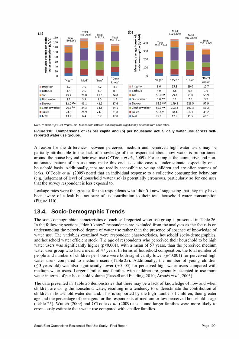
"High" "Med" "Low""Don't know"
Irrigation 4.2 7.5 8.2 4.5
Bathtub 1.5 2.6 1.7 0.8
Tap 25.7 28.8 25.3 24.8
Dishwasher 2.1 3.3 2.5 1.4
Shower 33.0 49.1 42.9 37.6
Clotheswasher 26.6 34.3 34.8 24.1
Toilet 23.8 24.9 24.0 21.8
Leak 13.2 6.4 3.2 17.8
0
20
40
60
80
100
120
140
160
Measured average per cap
ita
water consumption (L/p/d) Total
130 L/p/d
Total 156 L/p/d
Total 132 L/p/d
Total 143 L/p/d
(a)
*****
"High" "Med" "Low""Don't
know"
Irrigation 8.6 15.3 19.0 10.7
Bathtub 4.0 8.8 6.4 1.6
Tap 58.0 79.4 71.0 55.9
Dishwasher 5.0 9.1 7.3 3.9
Shower 82.5 149.8 126.5 97.9
Clotheswasher 62.3 103.8 101.3 53.2
Toilet 53.4 68.1 64.1 49.2
Leak 29.9 17.9 11.5 60.1
0
100
200
300
400
Measured average household
water consumption (L/hh/d)
Total 301 L/hh/d
Total 452 L/hh/d
Total 333 L/hh/d
Total 407 L/hh/d
(b)
*****
****
*
Note. *p<0.05,**p<0.01 ***p<0.001; Means with different subscripts are significantly different from each other.
Figure 110: Comparisons of (a) per capita and (b) per household actual daily water use across self-reported water use groups.
A reason for the differences between perceived medium and perceived high water users may be partially attributable to the lack of knowledge of the respondent about how water is proportioned around the house beyond their own use (O’Toole et al., 2009). For example, the cumulative and non-automated nature of tap use may make this end use quite easy to underestimate, especially on a household basis. Additionally, taps are readily accessible to young children and are often sources of leaks. O’Toole et al. (2009) noted that an individual response to a collective consumption behaviour (e.g. judgement of level of household water use) is potentially erroneous, particularly so for end uses that the survey respondent is less exposed to.
Leakage rates were the greatest for the respondents who ‘didn’t know’ suggesting that they may have been aware of a leak but not sure of its contribution to their total household water consumption (Figure 110).
13.4. Socio-Demographic Trends The socio-demographic characteristics of each self-reported water use group is presented in Table 26. In the following sections, “don’t know” respondents are excluded from the analyses as the focus is on understanding the perceived degree of water use rather than the presence of absence of knowledge of water use. The variables examined were respondent characteristics, household socio-demographics, and household water efficient stock. The age of respondents who perceived their household to be high water users was significantly higher (p<0.001), with a mean of 57 years, than the perceived medium water user group who had a mean of 47 years. In terms of household composition, the total number of people and number of children per house were both significantly lower (p<0.001) for perceived high water users compared to medium users (Table 25). Additionally, the number of young children (≤ 3 years old) was also significantly lower (p<0.05) for perceived high water users compared with medium water users. Larger families and families with children are generally accepted to use more water in terms of per household volume (Russell and Fielding, 2010; Arbués et al., 2003).
The data presented in Table 26 demonstrates that there may be a lack of knowledge of how and when children are using the household water, resulting in a tendency to underestimate the contribution of children in household water demand. This is supported by the high number of children, their greater age and the percentage of teenagers for the respondents of medium or low perceived household usage (Table 25). Wutich (2009) and O’Toole et al. (2009) also found larger families were more likely to erroneously estimate their water use compared with smaller families.
South East Queensland Residential End Use Study: Final Report Page 109
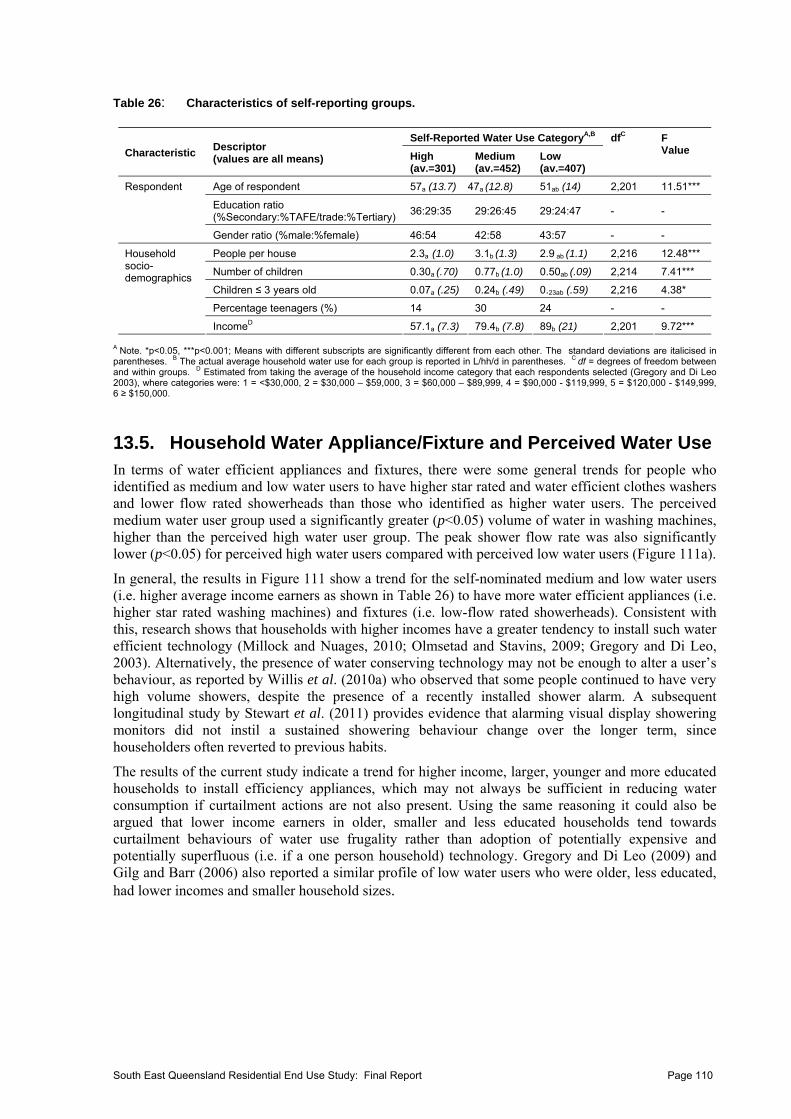
Table 26: Characteristics of self-reporting groups.
Self-Reported Water Use CategoryA,B
Characteristic Descriptor (values are all means) High
(av.=301) Medium (av.=452)
Low (av.=407)
dfC F Value
Age of respondent 57a (13.7) 47a (12.8) 51ab (14) 2,201 11.51***
Education ratio (%Secondary:%TAFE/trade:%Tertiary)
36:29:35 29:26:45 29:24:47 - -
Respondent
Gender ratio (%male:%female) 46:54 42:58 43:57 - -
People per house 2.3a (1.0) 3.1b
(1.3) 2.9 ab (1.1) 2,216 12.48***
Number of children 0.30a (.70) 0.77b
(1.0) 0.50ab (.09) 2,214 7.41***
Children ≤ 3 years old 0.07a (.25) 0.24b (.49) 0.23ab (.59) 2,216 4.38*
Percentage teenagers (%) 14 30 24 - -
Household socio-demographics
IncomeD 57.1a (7.3) 79.4b (7.8) 89b (21) 2,201 9.72***
A Note. *p<0.05, ***p<0.001; Means with different subscripts are significantly different from each other. The standard deviations are italicised in parentheses. B The actual average household water use for each group is reported in L/hh/d in parentheses. C df = degrees of freedom between and within groups. D Estimated from taking the average of the household income category that each respondents selected (Gregory and Di Leo 2003), where categories were: 1 = <$30,000, 2 = $30,000 – $59,000, 3 = $60,000 – $89,999, 4 = $90,000 - $119,999, 5 = $120,000 - $149,999, 6 ≥ $150,000.
13.5. Household Water Appliance/Fixture and Perceived Water Use In terms of water efficient appliances and fixtures, there were some general trends for people who identified as medium and low water users to have higher star rated and water efficient clothes washers and lower flow rated showerheads than those who identified as higher water users. The perceived medium water user group used a significantly greater (p<0.05) volume of water in washing machines, higher than the perceived high water user group. The peak shower flow rate was also significantly lower (p<0.05) for perceived high water users compared with perceived low water users (Figure 111a).
In general, the results in Figure 111 show a trend for the self-nominated medium and low water users (i.e. higher average income earners as shown in Table 26) to have more water efficient appliances (i.e. higher star rated washing machines) and fixtures (i.e. low-flow rated showerheads). Consistent with this, research shows that households with higher incomes have a greater tendency to install such water efficient technology (Millock and Nuages, 2010; Olmsetad and Stavins, 2009; Gregory and Di Leo, 2003). Alternatively, the presence of water conserving technology may not be enough to alter a user’s behaviour, as reported by Willis et al. (2010a) who observed that some people continued to have very high volume showers, despite the presence of a recently installed shower alarm. A subsequent longitudinal study by Stewart et al. (2011) provides evidence that alarming visual display showering monitors did not instil a sustained showering behaviour change over the longer term, since householders often reverted to previous habits.
The results of the current study indicate a trend for higher income, larger, younger and more educated households to install efficiency appliances, which may not always be sufficient in reducing water consumption if curtailment actions are not also present. Using the same reasoning it could also be argued that lower income earners in older, smaller and less educated households tend towards curtailment behaviours of water use frugality rather than adoption of potentially expensive and potentially superfluous (i.e. if a one person household) technology. Gregory and Di Leo (2009) and Gilg and Barr (2006) also reported a similar profile of low water users who were older, less educated, had lower incomes and smaller household sizes.
South East Queensland Residential End Use Study: Final Report Page 110
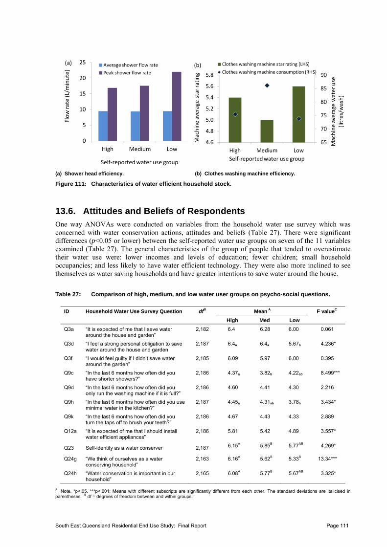
0
5
10
15
20
25
High Medium Low
Flow rate (L/minute)
Self‐reported water use group
Average shower flow rate
Peak shower flow rate
(a)
65
70
75
80
85
90
4.6
4.8
5.0
5.2
5.4
5.6
5.8
High Medium Low
Machine average water use
(litres/wash)
Machine average star rating
Self‐reported water use group
Clothes washing machine star rating (LHS)
Clothes washing machine consumption (RHS)(b)
(a) Shower head efficiency. (b) Clothes washing machine efficiency.
Figure 111: Characteristics of water efficient household stock.
13.6. Attitudes and Beliefs of Respondents One way ANOVAs were conducted on variables from the household water use survey which was concerned with water conservation actions, attitudes and beliefs (Table 27). There were significant differences (p<0.05 or lower) between the self-reported water use groups on seven of the 11 variables examined (Table 27). The general characteristics of the group of people that tended to overestimate their water use were: lower incomes and levels of education; fewer children; small household occupancies; and less likely to have water efficient technology. They were also more inclined to see themselves as water saving households and have greater intentions to save water around the house.
Table 27: Comparison of high, medium, and low water user groups on psycho-social questions.
ID Household Water Use Survey Question dfB Mean A F valueC
High Med Low
Q3a “It is expected of me that I save water around the house and garden”
2,182 6.4 6.28 6.00 0.061
Q3d “I feel a strong personal obligation to save water around the house and garden
2,187 6.4a 6.4a 5.67b 4.236*
Q3f “I would feel guilty if I didn’t save water around the garden”
2,185 6.09 5.97 6.00 0.395
Q9c “In the last 6 months how often did you have shorter showers?”
2,186 4.37a 3.82b 4.22ab 8.499***
Q9d “In the last 6 months how often did you only run the washing machine if it is full?”
2,186 4.60 4.41 4.30 2.216
Q9h “In the last 6 months how often did you use minimal water in the kitchen?”
2,187 4.45a 4.31ab 3.78b 3.434*
Q9k “In the last 6 months how often did you turn the taps off to brush your teeth?”
2,186 4.67 4.43 4.33 2.889
Q12a “It is expected of me that I should install water efficient appliances”
2,186 5.81 5.42 4.89 3.557*
Q23 Self-identity as a water conserver 2,187 6.15A 5.85B 5.77AB 4.269*
Q24g “We think of ourselves as a water conserving household”
2,163 6.16A 5.62B 5.33B 13.34***
Q24h “Water conservation is important in our household”
2,165 6.08A 5.77B 5.67AB 3.325*
A Note. *p<.05, ***p<.001; Means with different subscripts are significantly different from each other. The standard deviations are italicised in parentheses. B df = degrees of freedom between and within groups.
South East Queensland Residential End Use Study: Final Report Page 111
Conversely, the characteristics of the group who underestimated their water use were: higher incomes; larger families with young children; and more likely to have more water efficient technology including low-flow shower roses and higher star rated washing machines. This group tended to have lower self-identity as water conservers and demonstrated lower intentions to save water around the home. The ways in which this knowledge can inform future water demand management approaches can be grouped into soft or voluntary approaches where citizens are given the choice through education, awareness, incentives, etc., to change their consumption behaviours, or hard polices where mandatory tools such as restrictions are used to reduce demand (Jones et al., 2009).
13.7. Summary and Relevance of Findings Frequent and high volume water end uses such as clothes washing, showering and tap use were associated with the incorrect estimations of household consumption. Households that overestimate or underestimate their water use also differ in their socio-demographic and psycho-social profile, providing further clues for why the disparity between perceived and actual behaviour arises. This type of profiling can be used to formulate targeted water policy approaches such as educating citizens on their water use through feedback information and community-based social marketing. Heightened feedback to consumers on their households’ water consumption will improve their awareness and understanding of water use and help to encourage future water conservation behaviours.
The over- or under-estimation of water use by householders demonstrates that there cannot be exclusive reliance on individual household attitudes and beliefs to reduce water consumption. In some cases water demand management policy cannot rely solely on individual household attitudes and beliefs to reduce water consumption. Mandatory or hard measures such as water restrictions or tariff restructure are possibly more reliable in reducing residential demand, although a combination of regulation, efficiency appliances and behaviour change is likely to result in the best outcomes. A full discussion of results and policy implications relating to perceived versus actual (measured) household water use can be found in Beal et al. (2011a).
South East Queensland Residential End Use Study: Final Report Page 112
14. CLUSTERING WATER CONSUMPTION FLOW RATES
14.1. Introduction A challenge facing the water industry in optimising water resources available for use by the community is in the area of water leakage at the household level. Most Australian utilities are required to have water meter replacement programs, but there is still limited understanding of meter accuracy performance with in-situ age, particularly when considering its starting or minimum registration level (Qs or Qstart). Moreover, low flow residential water leakages are often not registered (i.e. Qevent<Qstart), and subsequently go undetected, by a typical water businesses aged fleet of conventional water meters. Currently, the entire community pays for this unaccounted water in the fixed and/or variable component of their water charges. This next section summarises the work performed using the SEQREUS data to determine the Qs and to subsequently allow a better understanding of post-meter residential water leakage, adequate meter sizing and the non-registration of meters.
14.2. Overview of Methods used to Determining Qs In order to categorise flow events, a software application was developed to assimilate data files containing household high resolution water consumption into various flow rate (L/hr) categories. The software was designed to read water usage from the data files (.txt file for each individual household covering a two-week period) and collate the water usage within the flow rate category range. A volume of water (litre per household per day, L/hh/d) for each flow rate category (e.g. < 5 L/hr, 5 ≤ 10 L/hr, up to 1,800+ L/hr; see Table 28) was then created. If the flow rate of a particular event was within the flow rate category, then the volume of that event was summed with others that belong to that category and total data was averaged for number of homes and total number of days of data. Results were then exported to an excel file where tables and charts were produced (i.e. volume in each flow rate category, per cent of water use in each flow rate category, cumulative volume and cumulative proportion of total consumption). As a note to readers, the smart meter used (i.e. modified Actaris CT-5) had a starting flow rate of 2 L/hr, so the recorded flows in the < 5 L/hr category do not accurately capture those very slow drips (< 2 L/hr) that may be occurring in the household.
14.3. Results and Discussion The average water usage and cumulative proportions of consumption are shown in Table 28. Data from this table are also presented graphically for the average and cumulative water consumption (Figure 112) and average and cumulative water use proportions (Figure 113). It is clear that there are three main ‘clusters’ of flow rate range categories (Table 28): - Flow rate range category Cluster 1 – this cluster denotes the first 11 categories (0 to ≤
100 L/hr) and contributes 10% of the total consumption. The lowest four categories (i.e. flow rates ≤ 30 L/hr) comprise 60% (or 19.5 L/hh/d) of the cluster, or 6% of the overall total consumption. The end uses associated with such low flows were mainly leaks, internal tap use, dishwasher, and some low-flow toilet, shower and clothes washing events.
- Flow rate range category Cluster 2 – this cluster represents the middle nine categories (100 ≤ 1,000 L/hr) and contributes to 80% of the total consumption. In particular, the categories between 300 ≤ 700 L/hr comprise 57% (or 148.8 L/hh/d) of the cluster, or 45% of the overall total consumption. The end uses associated with these flow rates were typically shower, clothes washing, full flush toilet use, external tap use, and irrigation.
- Flow rate range category Cluster 3 – this cluster denotes the last nine categories (1,000 < 1,800 L/hr) and contributes to 10% of the total consumption. The end uses associated with high flow rates included shower, clothes washing, external tap use, irrigation and uncommon water usage (e.g. service break leaks).
South East Queensland Residential End Use Study: Final Report Page 113
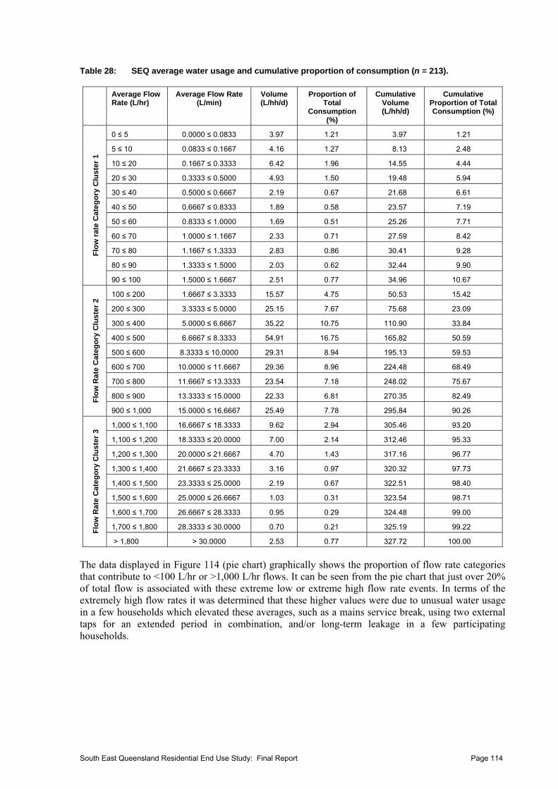
Table 28: SEQ average water usage and cumulative proportion of consumption (n = 213).
Average Flow Rate (L/hr)
Average Flow Rate (L/min)
Volume (L/hh/d)
Proportion of Total
Consumption (%)
Cumulative Volume (L/hh/d)
Cumulative Proportion of Total Consumption (%)
0 ≤ 5 0.0000 ≤ 0.0833 3.97 1.21 3.97 1.21
5 ≤ 10 0.0833 ≤ 0.1667 4.16 1.27 8.13 2.48
10 ≤ 20 0.1667 ≤ 0.3333 6.42 1.96 14.55 4.44
20 ≤ 30 0.3333 ≤ 0.5000 4.93 1.50 19.48 5.94
30 ≤ 40 0.5000 ≤ 0.6667 2.19 0.67 21.68 6.61
40 ≤ 50 0.6667 ≤ 0.8333 1.89 0.58 23.57 7.19
50 ≤ 60 0.8333 ≤ 1.0000 1.69 0.51 25.26 7.71
60 ≤ 70 1.0000 ≤ 1.1667 2.33 0.71 27.59 8.42
70 ≤ 80 1.1667 ≤ 1.3333 2.83 0.86 30.41 9.28
80 ≤ 90 1.3333 ≤ 1.5000 2.03 0.62 32.44 9.90
Flo
w r
ate
Cat
eg
ory
Clu
ste
r 1
90 ≤ 100 1.5000 ≤ 1.6667 2.51 0.77 34.96 10.67
100 ≤ 200 1.6667 ≤ 3.3333 15.57 4.75 50.53 15.42
200 ≤ 300 3.3333 ≤ 5.0000 25.15 7.67 75.68 23.09
300 ≤ 400 5.0000 ≤ 6.6667 35.22 10.75 110.90 33.84
400 ≤ 500 6.6667 ≤ 8.3333 54.91 16.75 165.82 50.59
500 ≤ 600 8.3333 ≤ 10.0000 29.31 8.94 195.13 59.53
600 ≤ 700 10.0000 ≤ 11.6667 29.36 8.96 224.48 68.49
700 ≤ 800 11.6667 ≤ 13.3333 23.54 7.18 248.02 75.67
800 ≤ 900 13.3333 ≤ 15.0000 22.33 6.81 270.35 82.49 Flo
w R
ate
Ca
teg
ory
Clu
ster
2
900 ≤ 1,000 15.0000 ≤ 16.6667 25.49 7.78 295.84 90.26
1,000 ≤ 1,100 16.6667 ≤ 18.3333 9.62 2.94 305.46 93.20
1,100 ≤ 1,200 18.3333 ≤ 20.0000 7.00 2.14 312.46 95.33
1,200 ≤ 1,300 20.0000 ≤ 21.6667 4.70 1.43 317.16 96.77
1,300 ≤ 1,400 21.6667 ≤ 23.3333 3.16 0.97 320.32 97.73
1,400 ≤ 1,500 23.3333 ≤ 25.0000 2.19 0.67 322.51 98.40
1,500 ≤ 1,600 25.0000 ≤ 26.6667 1.03 0.31 323.54 98.71
1,600 ≤ 1,700 26.6667 ≤ 28.3333 0.95 0.29 324.48 99.00
1,700 ≤ 1,800 28.3333 ≤ 30.0000 0.70 0.21 325.19 99.22 Flo
w R
ate
Ca
teg
ory
Clu
ster
3
> 1,800 > 30.0000 2.53 0.77 327.72 100.00
The data displayed in Figure 114 (pie chart) graphically shows the proportion of flow rate categories that contribute to <100 L/hr or >1,000 L/hr flows. It can be seen from the pie chart that just over 20% of total flow is associated with these extreme low or extreme high flow rate events. In terms of the extremely high flow rates it was determined that these higher values were due to unusual water usage in a few households which elevated these averages, such as a mains service break, using two external taps for an extended period in combination, and/or long-term leakage in a few participating households.
South East Queensland Residential End Use Study: Final Report Page 114
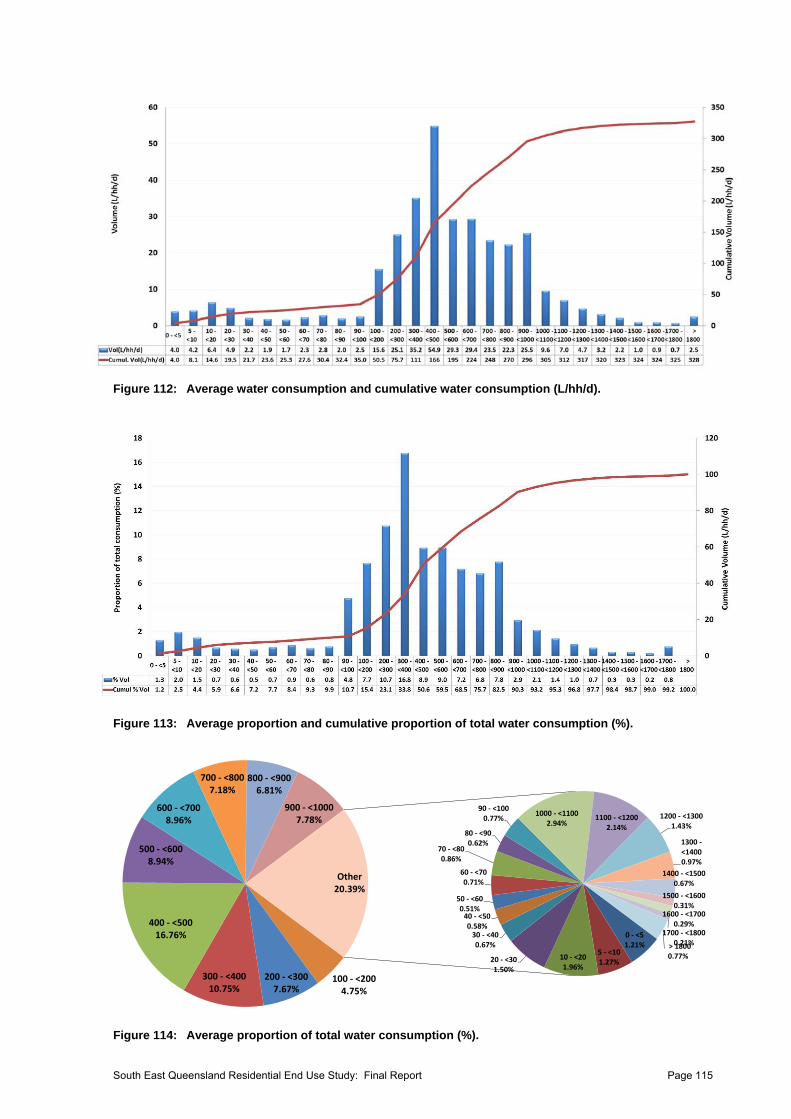
Figure 112: Average water consumption and cumulative water consumption (L/hh/d).
Figure 113: Average proportion and cumulative proportion of total water consumption (%).
0 ‐ <5 1.21%
5 ‐ <10 1.27%
10 ‐ <20 1.96%
20 ‐ <30 1.50%
30 ‐ <40 0.67%
40 ‐ <50 0.58%
50 ‐ <60 0.51%
60 ‐ <700.71%
70 ‐ <80 0.86%
80 ‐ <90 0.62%
90 ‐ <100 0.77%
100 ‐ <200 4.75%
200 ‐ <3007.67%
300 ‐ <40010.75%
400 ‐ <500 16.76%
500 ‐ <600 8.94%
600 ‐ <700 8.96%
700 ‐ <800 7.18%
800 ‐ <900 6.81%
900 ‐ <1000 7.78%
1000 ‐ <1100 2.94%
1100 ‐ <1200 2.14%
1200 ‐ <1300 1.43%
1300 ‐<1400 0.97%
1400 ‐ <15000.67%
1500 ‐ <16000.31%
1600 ‐ <17000.29%
1700 ‐ <18000.21%> 1800
0.77%
Other20.39%
Figure 114: Average proportion of total water consumption (%).
South East Queensland Residential End Use Study: Final Report Page 115
15. ENERGY DEMAND FROM WATER END USES
15.1. Introduction The conflict between water use and associated energy consumption is often referred to as the water-energy nexus. This is particularly relevant in an urban context as studies continue to demonstrate the significant role that the urban resident plays in consuming water and energy resources (Kenway et al., 2008; Lenzen and Peters, 2010; Kenway et al., 2011). Managing such interconnected resources has significant implications on the savings (or production) of greenhouse gas emissions (Kenway et al., 2011; Golden et al., 2010). As Fidar et al. (2010) and Maas (2009) observe, managing water demand through water efficient technology and behavioural changes has strong implications for reducing greenhouse gas emissions as well as conserving potable water supplies. This argument becomes stronger when one considers the acceleration of economic development and subsequent rise in living standards in some developing countries (Pakula and Stamminger, 2010).
The following section presents an overview of the methodology and some preliminary results obtained from analysing the energy requirements and resultant greenhouse gas emissions from residential water use appliances and fixtures (e.g. shower, tap, clothes washer and dishwasher).
15.2. Overview of Methods There were two major components to the methods: (1) determining water, energy and carbon emissions from measured water end uses; and (2) calculating the optimal combination of intervention solutions (e.g. cost effective energy-efficient options) to reduce carbon emissions from water end uses. A sub-sample of homes that had energy information captured during the household stock audit from the SEQREUS was used to determine the water (and energy) demand, thus, the water consumption values presented in section 15.5 will be slightly different than those reported for the full SEQREUS sample in earlier sections of this report. The sub-sample size was 211 homes; however, the sample was lower (n=189) for clothes washers and dishwashers due to some missing stock appliance data (e.g. information on clothes washer cycle temperatures and dishwasher models).
15.3. Calculating Energy Demand and Carbon Emissions
15.3.1. Determining Energy Consumption from End Use Data
Calculations shown in Table 29 were applied to the measured and published water and energy data described above to predict energy consumption for each end use in each household in the study. The mean, median, standard deviation and 95% confidence intervals are reported for each end use to characterise the variation and uncertainties of energy demand data across households and end uses. Units are reported in kilowatt hours per person per year (kWh/p/y). Note that the source of data for calculations were taken from Australian Government (2011, 2010a, 2010b) and Kenway et al. (2008) when not provided directly from household water stock audit.
Clothes washers (CW) are one of the most ubiquitous household appliances in the western world and are in use in an estimated 97% of Australian homes (Paluka and Stamminger, 2010). In calculating the energy demand from clothes washers, a number of issues need to be considered. Many of the later model machines have a horizontal axis (or are front loading machines) and only have a single, cold water tap connection to the machine, and thus heat water internally. In contrast, the older models tend to have vertical axis (or are top loading machines); they have a larger capacity and dual water connections (i.e. hot and cold tap connections to the machine). In this configuration, hot water is sourced from the external hot water service. As also observed by others, (Willis et al., 2011; Paluka and Stamminger, 2010; Flower, 2009; Kenway et al., 2008), the wide variety of heating, water connection, and loading configurations of clothes washers mean that the water and energy demands can vary markedly between the machines. The proportion of hot and cold water needs to be considered, along with a comparison between the energy demand from the internal heating and the energy demand from the HWS heating.
South East Queensland Residential End Use Study: Final Report Page 116
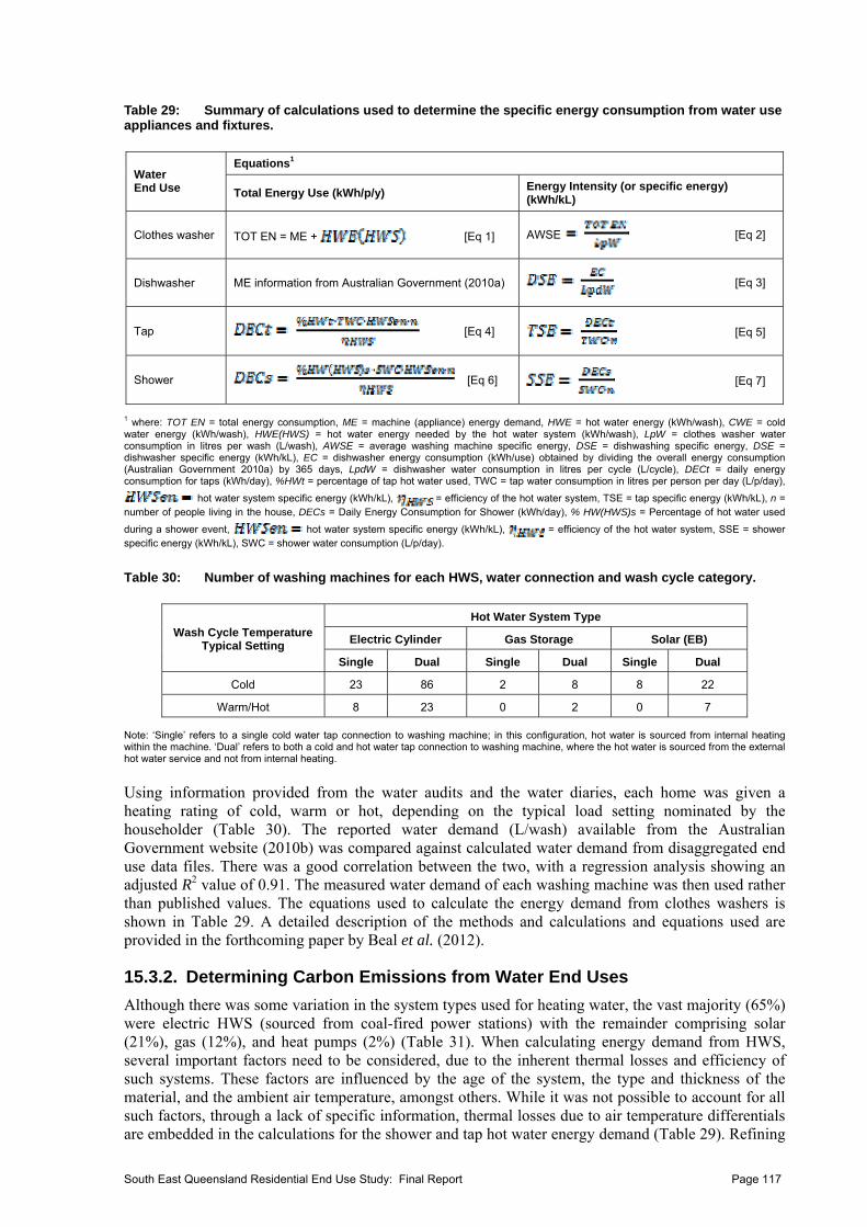
Table 29: Summary of calculations used to determine the specific energy consumption from water use appliances and fixtures.
Equations1 Water End Use Total Energy Use (kWh/p/y)
Energy Intensity (or specific energy) (kWh/kL)
Clothes washer TOT EN = ME + [Eq 1] AWSE [Eq 2]
Dishwasher ME information from Australian Government (2010a) [Eq 3]
Tap [Eq 4] [Eq 5]
Shower [Eq 6] [Eq 7]
1 where: TOT EN = total energy consumption, ME = machine (appliance) energy demand, HWE = hot water energy (kWh/wash), CWE = cold water energy (kWh/wash), HWE(HWS) = hot water energy needed by the hot water system (kWh/wash), LpW = clothes washer water consumption in litres per wash (L/wash), AWSE = average washing machine specific energy, DSE = dishwashing specific energy, DSE = dishwasher specific energy (kWh/kL), EC = dishwasher energy consumption (kWh/use) obtained by dividing the overall energy consumption (Australian Government 2010a) by 365 days, LpdW = dishwasher water consumption in litres per cycle (L/cycle), DECt = daily energy consumption for taps (kWh/day), %HWt = percentage of tap hot water used, TWC = tap water consumption in litres per person per day (L/p/day),
hot water system specific energy (kWh/kL), = efficiency of the hot water system, TSE = tap specific energy (kWh/kL), n = number of people living in the house, DECs = Daily Energy Consumption for Shower (kWh/day), % HW(HWS)s = Percentage of hot water used
during a shower event, hot water system specific energy (kWh/kL), = efficiency of the hot water system, SSE = shower specific energy (kWh/kL), SWC = shower water consumption (L/p/day).
Table 30: Number of washing machines for each HWS, water connection and wash cycle category.
Hot Water System Type
Electric Cylinder Gas Storage Solar (EB) Wash Cycle Temperature
Typical Setting
Single Dual Single Dual Single Dual
Cold 23 86 2 8 8 22
Warm/Hot 8 23 0 2 0 7 Note: ‘Single’ refers to a single cold water tap connection to washing machine; in this configuration, hot water is sourced from internal heating within the machine. ‘Dual’ refers to both a cold and hot water tap connection to washing machine, where the hot water is sourced from the external hot water service and not from internal heating.
Using information provided from the water audits and the water diaries, each home was given a heating rating of cold, warm or hot, depending on the typical load setting nominated by the householder (Table 30). The reported water demand (L/wash) available from the Australian Government website (2010b) was compared against calculated water demand from disaggregated end use data files. There was a good correlation between the two, with a regression analysis showing an adjusted R2 value of 0.91. The measured water demand of each washing machine was then used rather than published values. The equations used to calculate the energy demand from clothes washers is shown in Table 29. A detailed description of the methods and calculations and equations used are provided in the forthcoming paper by Beal et al. (2012).
15.3.2. Determining Carbon Emissions from Water End Uses
Although there was some variation in the system types used for heating water, the vast majority (65%) were electric HWS (sourced from coal-fired power stations) with the remainder comprising solar (21%), gas (12%), and heat pumps (2%) (Table 31). When calculating energy demand from HWS, several important factors need to be considered, due to the inherent thermal losses and efficiency of such systems. These factors are influenced by the age of the system, the type and thickness of the material, and the ambient air temperature, amongst others. While it was not possible to account for all such factors, through a lack of specific information, thermal losses due to air temperature differentials are embedded in the calculations for the shower and tap hot water energy demand (Table 29). Refining
South East Queensland Residential End Use Study: Final Report Page 117
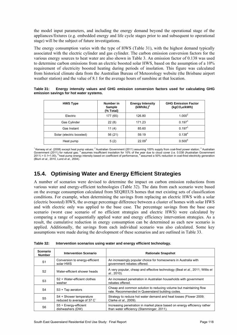
South East Queensland Residential End Use Study: Final Report Page 118
the model input parameters, and including the energy demand beyond the operational stage of the appliances/fixtures (e.g. embedded energy and life cycle stages prior to and subsequent to operational stage) will be the subject of future investigations.
The energy consumption varies with the type of HWS (Table 31), with the highest demand typically associated with the electric cylinder and gas cylinder. The carbon emission conversion factors for the various energy sources to heat water are also shown in Table 3. An emission factor of 0.138 was used to determine carbon emissions from an electric boosted solar HWS, based on the assumption of a 10% requirement of electricity boosted heating during periods of insolation. This figure was calculated from historical climate data from the Australian Bureau of Meteorology website (the Brisbane airport weather station) and the value of 8.1 for the average hours of sunshine at that location.
Table 31: Energy intensity values and GHG emission conversion factors used for calculating GHG emission savings for hot water systems.
HWS Type Number in Sample
(% Total)
Energy Intensity (kWh/kL)1
GHG Emission Factor (kgCO2e/kWh)
Electric 177 (65) 126.80 1.0002
Gas Cylinder 22 (8) 171.23 0.1973
Gas Instant 11 (4) 85.60 0.1973
Solar (electric boosted) 56 (21) 59.19 0.1384
Heat pump 5 (2) 22.095 0.5006
1 Kenway et al. (2008) except heat pump values; 2 Australian Government (2011) assuming 100% supply from coal-fired power station; 3 Australian Government (2011) for natural gas; 4 assumes insufficient insolation for 10% of the year due to cloud cover (i.e. 0.038 (Australian Government 2011) + 0.1×1.00), 5 heat pump energy intensity based on coefficient of performance, 6 assumed a 50% reduction in coal-fired electricity generation (Blum et al., 2010, Lund et al., 2004).
15.4. Optimising Water and Energy Efficient Strategies A number of scenarios were devised to determine the impact on carbon emission reductions from various water and energy-efficient technologies (Table 32). The data from each scenario were based on the average consumption calculated from SEQREUS homes that met existing sets of classification conditions. For example, when determining the savings from replacing an electric HWS with a solar (electric boosted) HWS, the average percentage difference between a cluster of homes with solar HWS and with electric only was applied to the base case. The percentage savings from the base case scenario (worst case scenario of no efficient strategies and electric HWS) were calculated by comparing a range of sequentially applied water and energy efficiency intervention strategies. As a result, the cumulative reduction in energy consumption can be determined as each new scenario is applied. Additionally, the savings from each individual scenario was also calculated. Some key assumptions were made during the development of these scenarios and are outlined in Table 33.
Table 32: Intervention scenarios using water and energy efficient technology.
Scenario Number
Intervention Scenario Rationale Snapshot
S1 Conversion to energy-efficient solar HWS
An increasingly popular choice for homeowners in Australia with government rebates offered.
S2 Water-efficient shower heads A very popular, cheap and effective technology (Beal et al., 2011; Willis et al., 2010).
S3 S2 + Water-efficient clothes washer
An increased penetration in Australian households with government rebates offered.
S4 S3 + Tap aerators Cheap and common solution to reducing volume but maintaining flow rate. Recommended in Queensland building codes.
S5 S4 + Shower temperature reduced to average of 37 C˚
Strategy to reduce hot water demand and heat losses (Flower 2009; Clarke et al., 2009).
S6 S5 + Energy-efficient dishwashers (DW)
Increasing penetration in market place based on energy efficiency rather than water efficiency (Stamminger, 2011).
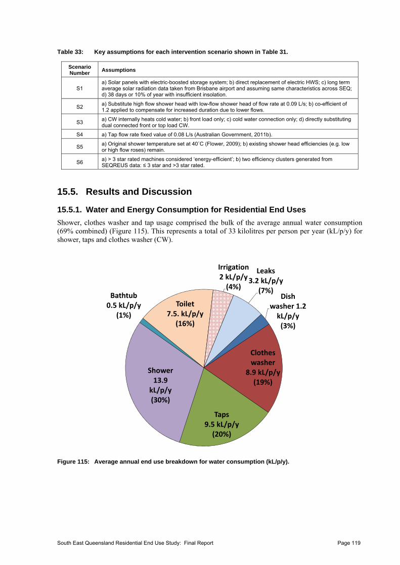
Table 33: Key assumptions for each intervention scenario shown in Table 31.
Scenario Number
Assumptions
S1 a) Solar panels with electric-boosted storage system; b) direct replacement of electric HWS; c) long term average solar radiation data taken from Brisbane airport and assuming same characteristics across SEQ; d) 38 days or 10% of year with insufficient insolation.
S2 a) Substitute high flow shower head with low-flow shower head of flow rate at 0.09 L/s; b) co-efficient of 1.2 applied to compensate for increased duration due to lower flows.
S3 a) CW internally heats cold water; b) front load only; c) cold water connection only; d) directly substituting dual connected front or top load CW.
S4 a) Tap flow rate fixed value of 0.08 L/s (Australian Government, 2011b).
S5 a) Original shower temperature set at 40˚C (Flower, 2009); b) existing shower head efficiencies (e.g. low or high flow roses) remain.
S6 a) > 3 star rated machines considered ‘energy-efficient’; b) two efficiency clusters generated from SEQREUS data: ≤ 3 star and >3 star rated.
15.5. Results and Discussion
15.5.1. Water and Energy Consumption for Residential End Uses
Shower, clothes washer and tap usage comprised the bulk of the average annual water consumption (69% combined) (Figure 115). This represents a total of 33 kilolitres per person per year (kL/p/y) for shower, taps and clothes washer (CW).
Dish washer 1.2 kL/p/y(3%)
Clothes washer
8.9 kL/p/y (19%)
Taps 9.5 kL/p/y(20%)
Shower13.9 kL/p/y(30%)
Bathtub0.5 kL/p/y
(1%)
Toilet7.5. kL/p/y
(16%)
Irrigation2 kL/p/y(4%)
Leaks3.2 kL/p/y
(7%)
Figure 115: Average annual end use breakdown for water consumption (kL/p/y).
South East Queensland Residential End Use Study: Final Report Page 119
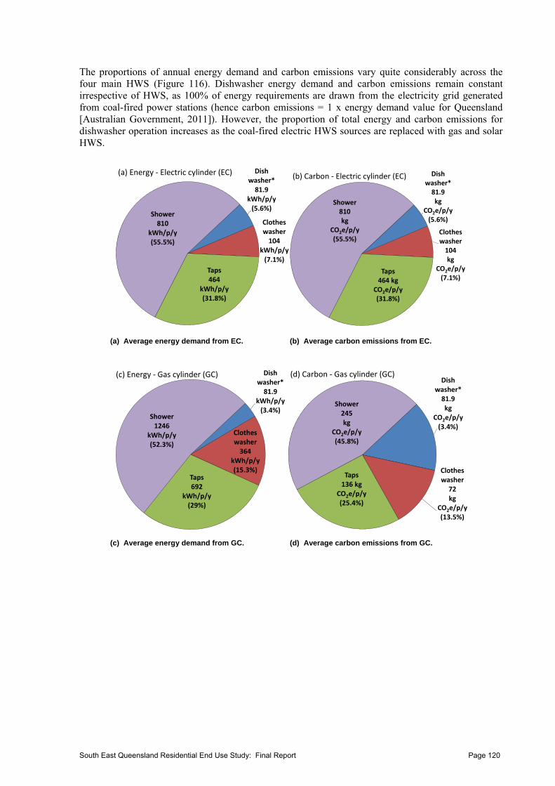
The proportions of annual energy demand and carbon emissions vary quite considerably across the four main HWS (Figure 116). Dishwasher energy demand and carbon emissions remain constant irrespective of HWS, as 100% of energy requirements are drawn from the electricity grid generated from coal-fired power stations (hence carbon emissions = 1 x energy demand value for Queensland [Australian Government, 2011]). However, the proportion of total energy and carbon emissions for dishwasher operation increases as the coal-fired electric HWS sources are replaced with gas and solar HWS.
Dish
washer* 81.9
kWh/p/y(5.6%)
Clothes washer 104
kWh/p/y (7.1%)
Taps 464
kWh/p/y(31.8%)
Shower810
kWh/p/y(55.5%)
(a) Energy ‐ Electric cylinder (EC) Dish washer* 81.9 kg
CO2e/p/y(5.6%)
Clothes washer 104 kg
CO2e/p/y (7.1%)
Taps 464 kg
CO2e/p/y(31.8%)
Shower 810 kg
CO2e/p/y (55.5%)
(b) Carbon ‐ Electric cylinder (EC)
(a) Average energy demand from EC. (b) Average carbon emissions from EC.
Dish washer* 81.9
kWh/p/y(3.4%)
Clothes washer 364
kWh/p/y (15.3%)
Taps 692
kWh/p/y(29%)
Shower1246
kWh/p/y(52.3%)
(c) Energy ‐ Gas cylinder (GC)Dish
washer* 81.9 kg
CO2e/p/y(3.4%)
Clothes washer 72 kg
CO2e/p/y (13.5%)
Taps 136 kg
CO2e/p/y(25.4%)
Shower 245 kg
CO2e/p/y (45.8%)
(d) Carbon ‐ Gas cylinder (GC)
(c) Average energy demand from GC. (d) Average carbon emissions from GC.
South East Queensland Residential End Use Study: Final Report Page 120
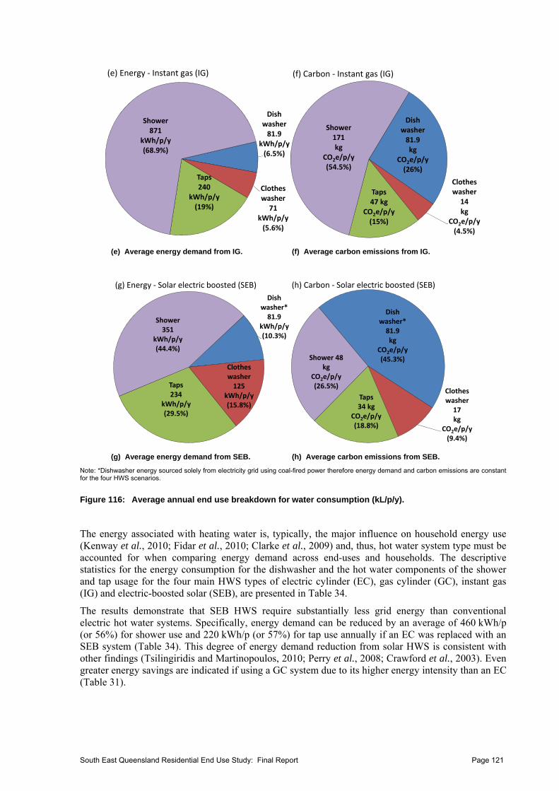
Dish washer 81.9
kWh/p/y(6.5%)
Clothes washer 71
kWh/p/y (5.6%)
Taps 240
kWh/p/y(19%)
Shower871
kWh/p/y(68.9%)
(e) Energy ‐ Instant gas (IG)
Dish washer 81.9 kg
CO2e/p/y(26%)
Clothes washer 14 kg
CO2e/p/y (4.5%)
Taps 47 kg
CO2e/p/y(15%)
Shower 171 kg
CO2e/p/y (54.5%)
(f) Carbon ‐ Instant gas (IG)
(e) Average energy demand from IG. (f) Average carbon emissions from IG.
Dish washer* 81.9
kWh/p/y(10.3%)
Clothes washer 125
kWh/p/y (15.8%)
Taps 234
kWh/p/y(29.5%)
Shower351
kWh/p/y(44.4%)
(g) Energy ‐ Solar electric boosted (SEB)
Dish washer* 81.9 kg
CO2e/p/y(45.3%)
Clothes washer 17kg
CO2e/p/y (9.4%)
Taps 34 kg
CO2e/p/y(18.8%)
Shower 48 kg
CO2e/p/y (26.5%)
(h) Carbon ‐ Solar electric boosted (SEB)
(g) Average energy demand from SEB. (h) Average carbon emissions from SEB.
Note: *Dishwasher energy sourced solely from electricity grid using coal-fired power therefore energy demand and carbon emissions are constant for the four HWS scenarios.
Figure 116: Average annual end use breakdown for water consumption (kL/p/y).
The energy associated with heating water is, typically, the major influence on household energy use (Kenway et al., 2010; Fidar et al., 2010; Clarke et al., 2009) and, thus, hot water system type must be accounted for when comparing energy demand across end-uses and households. The descriptive statistics for the energy consumption for the dishwasher and the hot water components of the shower and tap usage for the four main HWS types of electric cylinder (EC), gas cylinder (GC), instant gas (IG) and electric-boosted solar (SEB), are presented in Table 34.
The results demonstrate that SEB HWS require substantially less grid energy than conventional electric hot water systems. Specifically, energy demand can be reduced by an average of 460 kWh/p (or 56%) for shower use and 220 kWh/p (or 57%) for tap use annually if an EC was replaced with an SEB system (Table 34). This degree of energy demand reduction from solar HWS is consistent with other findings (Tsilingiridis and Martinopoulos, 2010; Perry et al., 2008; Crawford et al., 2003). Even greater energy savings are indicated if using a GC system due to its higher energy intensity than an EC (Table 31).
South East Queensland Residential End Use Study: Final Report Page 121
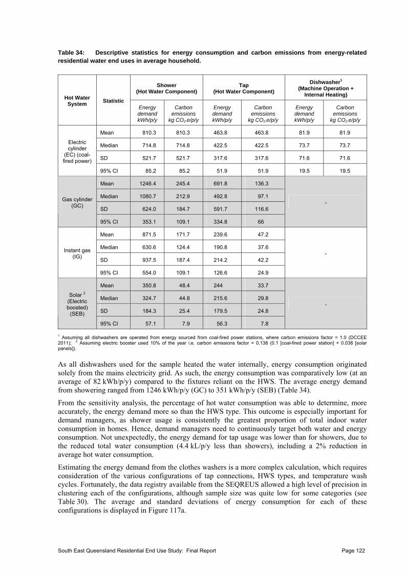
Table 34: Descriptive statistics for energy consumption and carbon emissions from energy-related residential water end uses in average household.
Shower (Hot Water Component)
Tap (Hot Water Component)
Dishwasher1
(Machine Operation + Internal Heating) Hot Water
System Statistic
Energy demand kWh/p/y
Carbon emissions
kg CO2-e/p/y
Energy demand kWh/p/y
Carbon emissions
kg CO2-e/p/y
Energy demand kWh/p/y
Carbon emissions
kg CO2-e/p/y
Mean 810.3 810.3 463.8 463.8 81.9 81.9
Median 714.8 714.8 422.5 422.5 73.7 73.7
SD 521.7 521.7 317.6 317.6 71.6 71.6
Electric cylinder
(EC) (coal-fired power)
95% CI 85.2 85.2 51.9 51.9 19.5 19.5
Mean 1246.4 245.4 691.8 136.3
Median 1080.7 212.9 492.8 97.1
SD 624.0 184.7 591.7 116.6
Gas cylinder (GC)
95% CI 353.1 109.1 334.8 66
-
Mean 871.5 171.7 239.6 47.2
Median 630.6 124.4 190.8 37.6
SD 937.5 187.4 214.2 42.2
Instant gas (IG)
95% CI 554.0 109.1 126.6 24.9
-
Mean 350.8 48.4 244 33.7
Median 324.7 44.8 215.6 29.8
SD 184.3 25.4 179.5 24.8
Solar 2 (Electric boosted)
(SEB)
95% CI 57.1 7.9 56.3 7.8
-
1 Assuming all dishwashers are operated from energy sourced from coal-fired power stations, where carbon emissions factor = 1.0 (DCCEE 2011); 2 Assuming electric booster used 10% of the year i.e. carbon emissions factor = 0.138 (0.1 [coal-fired power station] + 0.038 [solar panels]).
As all dishwashers used for the sample heated the water internally, energy consumption originated solely from the mains electricity grid. As such, the energy consumption was comparatively low (at an average of 82 kWh/p/y) compared to the fixtures reliant on the HWS. The average energy demand from showering ranged from 1246 kWh/p/y (GC) to 351 kWh/p/y (SEB) (Table 34).
From the sensitivity analysis, the percentage of hot water consumption was able to determine, more accurately, the energy demand more so than the HWS type. This outcome is especially important for demand managers, as shower usage is consistently the greatest proportion of total indoor water consumption in homes. Hence, demand managers need to continuously target both water and energy consumption. Not unexpectedly, the energy demand for tap usage was lower than for showers, due to the reduced total water consumption (4.4 kL/p/y less than showers), including a 2% reduction in average hot water consumption.
Estimating the energy demand from the clothes washers is a more complex calculation, which requires consideration of the various configurations of tap connections, HWS types, and temperature wash cycles. Fortunately, the data registry available from the SEQREUS allowed a high level of precision in clustering each of the configurations, although sample size was quite low for some categories (see Table 30). The average and standard deviations of energy consumption for each of these configurations is displayed in Figure 117a.
South East Queensland Residential End Use Study: Final Report Page 122
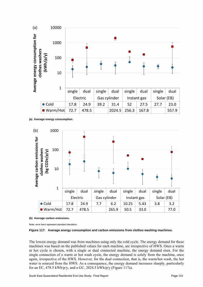
single dual single dual single dual single dual
Electric Gas cylinder Instant gas Solar (EB)
Cold 17.8 24.9 39.2 31.4 52 27.5 27.7 23.0
Warm/Hot 72.7 478.5 2024.5 256.3 167.8 557.9
1
10
100
1000
10000
Average energy consumption for
clothes washers
(kWh/p/y)
(a)
(a) Average energy consumption.
single dual single dual single dual single dual
Electric Gas cylinder Instant gas Solar (EB)
Cold 17.8 24.9 7.7 6.2 10.25 5.43 3.8 3.2
Warm/Hot 72.7 478.5 265.9 50.5 33.0 77.0
1
10
100
1000
Average carbon emissions for
clothes washers
(kg CO2e/p/y)
(b)
(b) Average carbon emissions.
Note: error bars represent standard deviation.
Figure 117: Average energy consumption and carbon emissions from clothes washing machines.
The lowest energy demand was from machines using only the cold cycle. The energy demand for these machines was based on the published values for each machine, are irrespective of HWS. Once a warm or hot cycle is chosen, with a single or dual connected machine, the energy demand rises. For the single connection of a warm or hot wash cycle, the energy demand is solely from the machine, once again, irrespective of the HWS. However, for the dual connection, that is, the warm/hot wash, the hot water is sourced from the HWS. As a consequence, the energy demand increases sharply, particularly for an EC, 478.5 kWh/p/y, and a GC, 2024.5 kWh/p/y (Figure 117a).
South East Queensland Residential End Use Study: Final Report Page 123
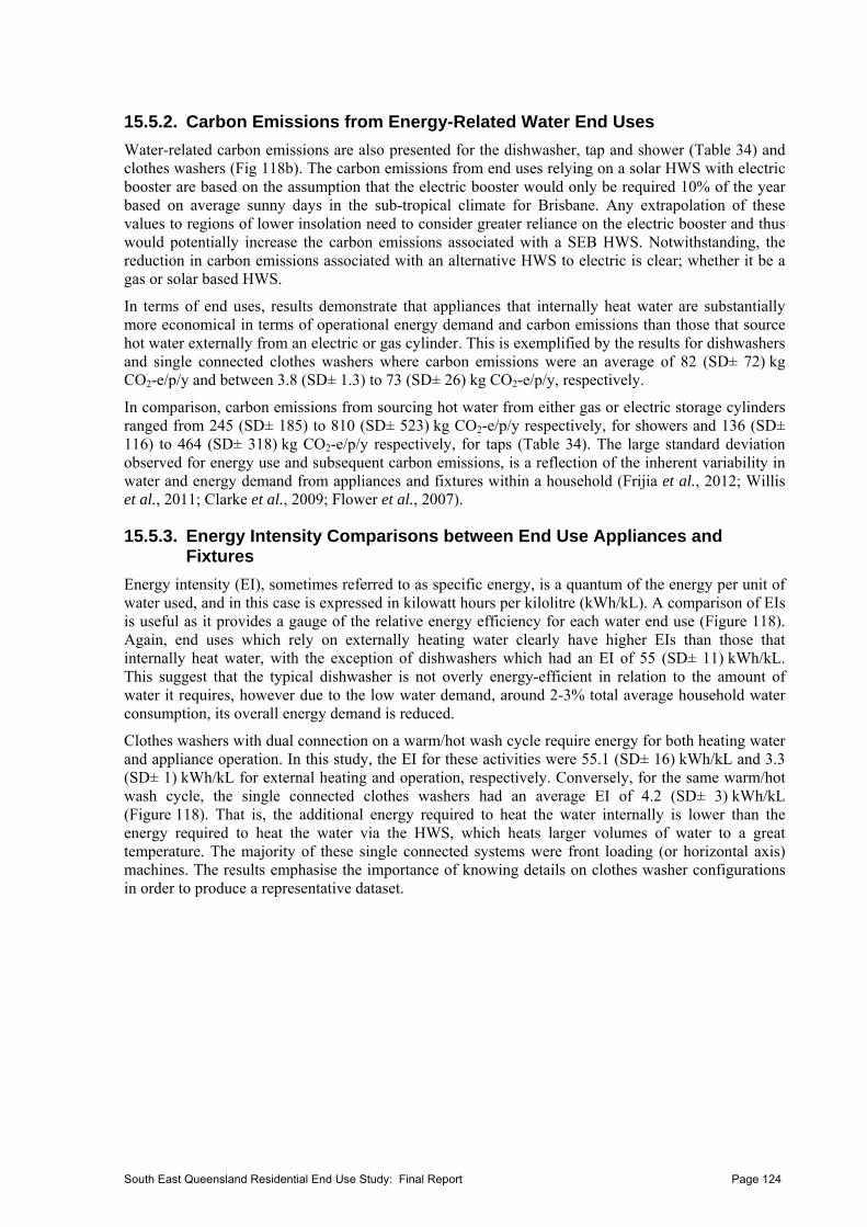
15.5.2. Carbon Emissions from Energy-Related Water End Uses
Water-related carbon emissions are also presented for the dishwasher, tap and shower (Table 34) and clothes washers (Fig 118b). The carbon emissions from end uses relying on a solar HWS with electric booster are based on the assumption that the electric booster would only be required 10% of the year based on average sunny days in the sub-tropical climate for Brisbane. Any extrapolation of these values to regions of lower insolation need to consider greater reliance on the electric booster and thus would potentially increase the carbon emissions associated with a SEB HWS. Notwithstanding, the reduction in carbon emissions associated with an alternative HWS to electric is clear; whether it be a gas or solar based HWS.
In terms of end uses, results demonstrate that appliances that internally heat water are substantially more economical in terms of operational energy demand and carbon emissions than those that source hot water externally from an electric or gas cylinder. This is exemplified by the results for dishwashers and single connected clothes washers where carbon emissions were an average of 82 (SD± 72) kg CO2-e/p/y and between 3.8 (SD± 1.3) to 73 (SD± 26) kg CO2-e/p/y, respectively.
In comparison, carbon emissions from sourcing hot water from either gas or electric storage cylinders ranged from 245 (SD± 185) to 810 (SD± 523) kg CO2-e/p/y respectively, for showers and 136 (SD± 116) to 464 (SD± 318) kg CO2-e/p/y respectively, for taps (Table 34). The large standard deviation observed for energy use and subsequent carbon emissions, is a reflection of the inherent variability in water and energy demand from appliances and fixtures within a household (Frijia et al., 2012; Willis et al., 2011; Clarke et al., 2009; Flower et al., 2007).
15.5.3. Energy Intensity Comparisons between End Use Appliances and Fixtures
Energy intensity (EI), sometimes referred to as specific energy, is a quantum of the energy per unit of water used, and in this case is expressed in kilowatt hours per kilolitre (kWh/kL). A comparison of EIs is useful as it provides a gauge of the relative energy efficiency for each water end use (Figure 118). Again, end uses which rely on externally heating water clearly have higher EIs than those that internally heat water, with the exception of dishwashers which had an EI of 55 (SD± 11) kWh/kL. This suggest that the typical dishwasher is not overly energy-efficient in relation to the amount of water it requires, however due to the low water demand, around 2-3% total average household water consumption, its overall energy demand is reduced.
Clothes washers with dual connection on a warm/hot wash cycle require energy for both heating water and appliance operation. In this study, the EI for these activities were 55.1 (SD± 16) kWh/kL and 3.3 (SD± 1) kWh/kL for external heating and operation, respectively. Conversely, for the same warm/hot wash cycle, the single connected clothes washers had an average EI of 4.2 (SD± 3) kWh/kL (Figure 118). That is, the additional energy required to heat the water internally is lower than the energy required to heat the water via the HWS, which heats larger volumes of water to a great temperature. The majority of these single connected systems were front loading (or horizontal axis) machines. The results emphasise the importance of knowing details on clothes washer configurations in order to produce a representative dataset.
South East Queensland Residential End Use Study: Final Report Page 124
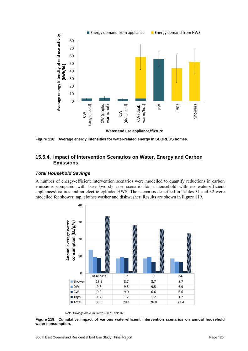
0
10
20
30
40
50
60
70
80
CW
(single, cold)
CW (single,
warm/hot)
CW
(dual, cold)
CW (dual,
warm/hot)
DW
Taps
Showers
Average energy intensity of end use activity
(kWh/kL)
Water end use appliance/fixture
Energy demand from appliance Energy demand from HWS
Figure 118: Average energy intensities for water-related energy in SEQREUS homes.
15.5.4. Impact of Intervention Scenarios on Water, Energy and Carbon Emissions
Total Household Savings
A number of energy-efficient intervention scenarios were modelled to quantify reductions in carbon emissions compared with base (worst) case scenario for a household with no water-efficient appliances/fixtures and an electric cylinder HWS. The scenarios described in Tables 31 and 32 were modelled for shower, tap, clothes washer and dishwasher. Results are shown in Figure 119.
Base case S2 S3 S4
Shower 13.9 8.7 8.7 8.7
DW 9.5 9.5 9.5 6.9
CW 9.0 9.0 6.6 6.6
Taps 1.2 1.2 1.2 1.2
Total 33.6 28.4 26.0 23.4
0
10
20
30
40
Annual average
water
consumption (kL/p/y)
Note: Savings are cumulative – see Table 32.
Figure 119: Cumulative impact of various water-efficient intervention scenarios on annual household water consumption.
South East Queensland Residential End Use Study: Final Report Page 125

Figure 119 shows the annual average water consumption starting with the base case using SEQREUS data from homes without any of the water-efficient technologies. Cumulative reductions are then shown as each scenario is applied (i.e. the final row in Figure 119 assumes all the previous scenarios are applied as well as installing a 4 star shower head). Results show that a savings of 10.2 kL/p/y can be achieved by installing a combination of water-efficient shower, tap and clothes washer stock. The water savings from efficient clothes washers are a little lower than reported elsewhere (e.g. Willis et al., 2011), and may be a function of elevated water usage for a small number of homes with high star-rated machines. Beal et al. (2011b) discuss the phenomenon where people with a high level of water-efficient stock do not necessarily exhibit water conserving behaviours (such as reducing the number of small loads) and this may also have been a factor in the observed lower water savings from homes with water-efficient clothes washers.
The annual household energy consumption and carbon emission savings was also predicted for various resource-efficient stock for two groups: (i) no change to an existing electric HWS (Figure 120a); and (ii) replacement of an electric HWs with a solar HWS (SEB) (Figure 120b and Figure 121). Both these scenarios have been presented to represent older/existing homes with retrofitted resource-efficient indoor stock but an existing EC HWS, and newer homes built under current building code sustainability requirements which would include both resource-efficient stock and an efficient HWS (in this case a SEB). Knowledge of the savings from both scenarios can assist in the decision making for developing future building development codes.
Base case S2 S3 S4 S5 S6
Shower 821 305 305 305 259 259
Taps 464 464 464 291 291 291
CW 252 252 45 45 45 45
DW 82 82 82 82 82 59
Total 1619 1103 896 723 677 654
1
10
100
1000
10000
Annual average energy consumption
EC H
WS (kW
h/p/y)
(a)
(a) Energy savings from an existing EC HWS + efficient stock.
South East Queensland Residential End Use Study: Final Report Page 126
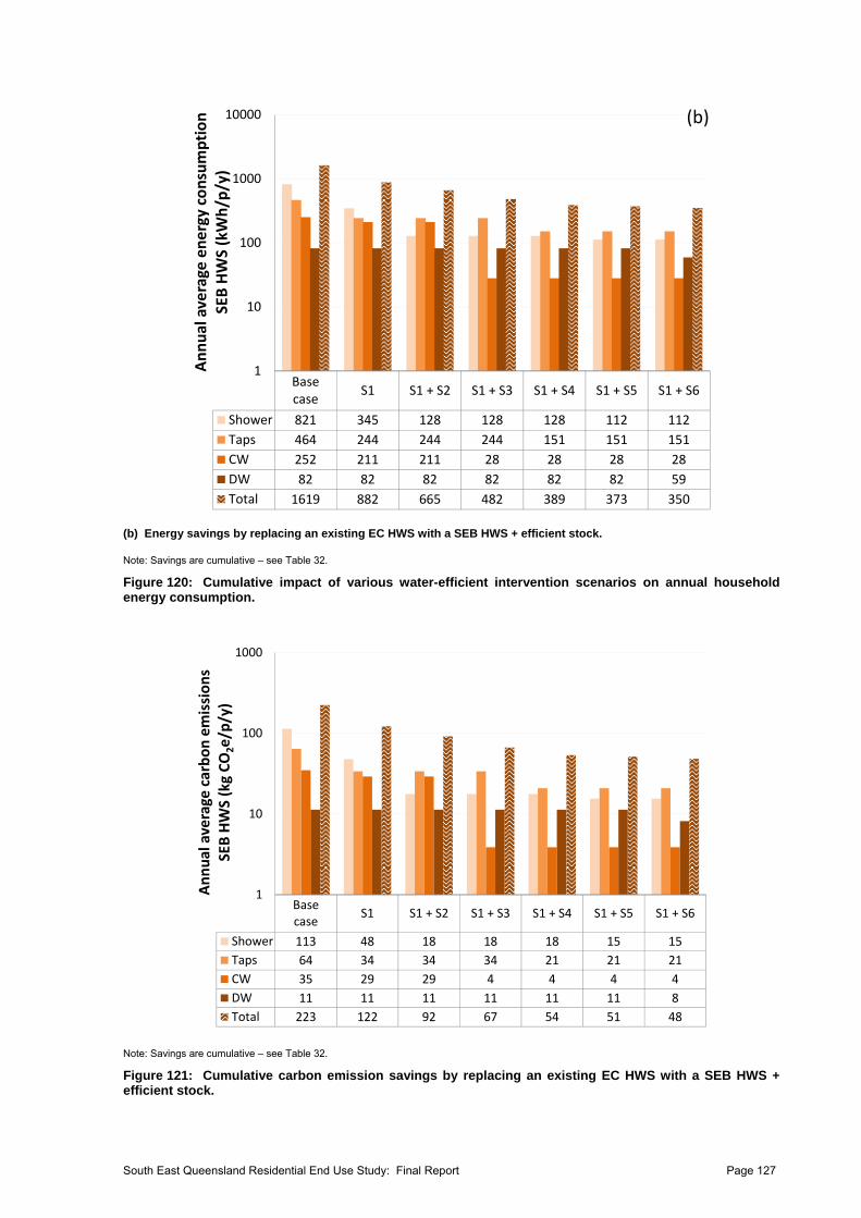
Basecase
S1 S1 + S2 S1 + S3 S1 + S4 S1 + S5 S1 + S6
Shower 821 345 128 128 128 112 112
Taps 464 244 244 244 151 151 151
CW 252 211 211 28 28 28 28
DW 82 82 82 82 82 82 59
Total 1619 882 665 482 389 373 350
1
10
100
1000
10000
Annual average energy consumption
SEB HWS (kWh/p/y)
(b)
(b) Energy savings by replacing an existing EC HWS with a SEB HWS + efficient stock.
Note: Savings are cumulative – see Table 32.
Figure 120: Cumulative impact of various water-efficient intervention scenarios on annual household energy consumption.
Basecase
S1 S1 + S2 S1 + S3 S1 + S4 S1 + S5 S1 + S6
Shower 113 48 18 18 18 15 15
Taps 64 34 34 34 21 21 21
CW 35 29 29 4 4 4 4
DW 11 11 11 11 11 11 8
Total 223 122 92 67 54 51 48
1
10
100
1000
Annual average carbon emissions
SEB HWS (kg CO2e/p/y)
Note: Savings are cumulative – see Table 32.
Figure 121: Cumulative carbon emission savings by replacing an existing EC HWS with a SEB HWS + efficient stock.
South East Queensland Residential End Use Study: Final Report Page 127
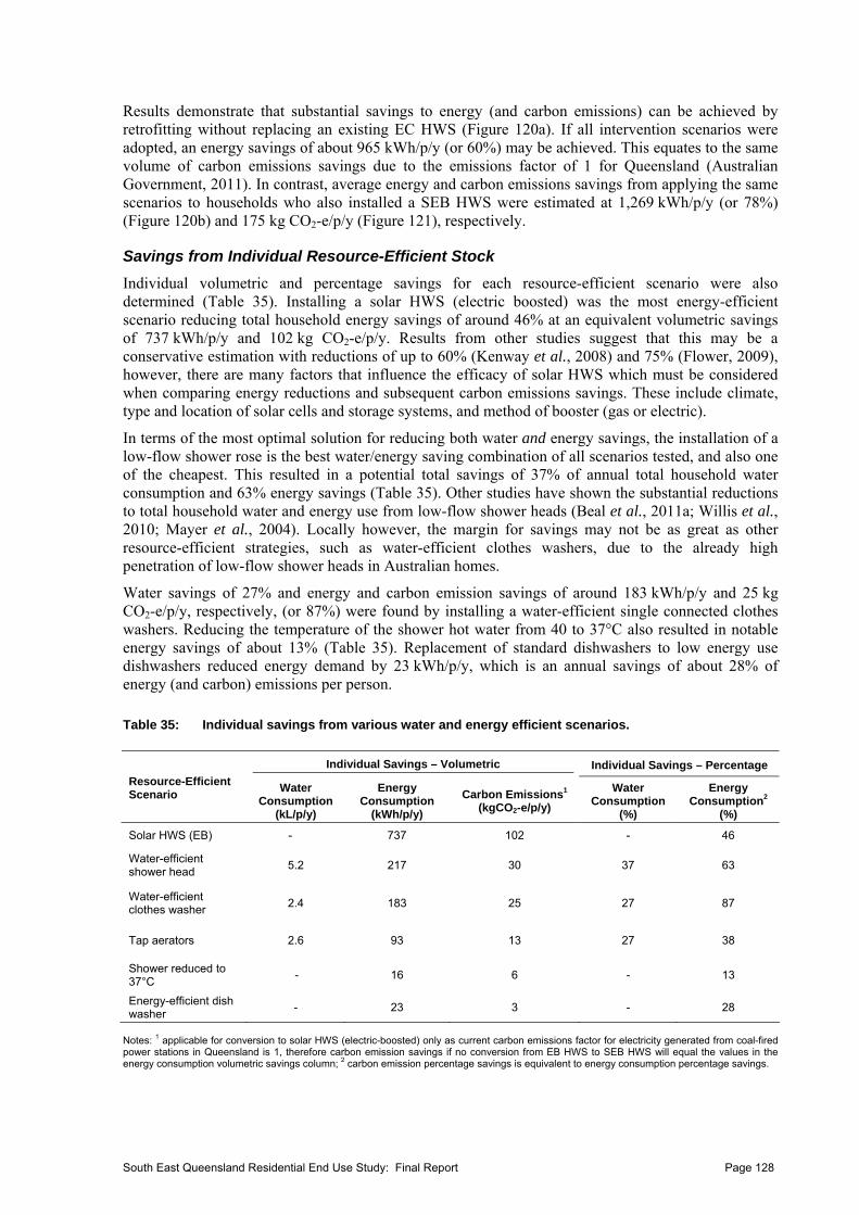
Results demonstrate that substantial savings to energy (and carbon emissions) can be achieved by retrofitting without replacing an existing EC HWS (Figure 120a). If all intervention scenarios were adopted, an energy savings of about 965 kWh/p/y (or 60%) may be achieved. This equates to the same volume of carbon emissions savings due to the emissions factor of 1 for Queensland (Australian Government, 2011). In contrast, average energy and carbon emissions savings from applying the same scenarios to households who also installed a SEB HWS were estimated at 1,269 kWh/p/y (or 78%) (Figure 120b) and 175 kg CO2-e/p/y (Figure 121), respectively.
Savings from Individual Resource-Efficient Stock
Individual volumetric and percentage savings for each resource-efficient scenario were also determined (Table 35). Installing a solar HWS (electric boosted) was the most energy-efficient scenario reducing total household energy savings of around 46% at an equivalent volumetric savings of 737 kWh/p/y and 102 kg CO2-e/p/y. Results from other studies suggest that this may be a conservative estimation with reductions of up to 60% (Kenway et al., 2008) and 75% (Flower, 2009), however, there are many factors that influence the efficacy of solar HWS which must be considered when comparing energy reductions and subsequent carbon emissions savings. These include climate, type and location of solar cells and storage systems, and method of booster (gas or electric).
In terms of the most optimal solution for reducing both water and energy savings, the installation of a low-flow shower rose is the best water/energy saving combination of all scenarios tested, and also one of the cheapest. This resulted in a potential total savings of 37% of annual total household water consumption and 63% energy savings (Table 35). Other studies have shown the substantial reductions to total household water and energy use from low-flow shower heads (Beal et al., 2011a; Willis et al., 2010; Mayer et al., 2004). Locally however, the margin for savings may not be as great as other resource-efficient strategies, such as water-efficient clothes washers, due to the already high penetration of low-flow shower heads in Australian homes.
Water savings of 27% and energy and carbon emission savings of around 183 kWh/p/y and 25 kg CO2-e/p/y, respectively, (or 87%) were found by installing a water-efficient single connected clothes washers. Reducing the temperature of the shower hot water from 40 to 37°C also resulted in notable energy savings of about 13% (Table 35). Replacement of standard dishwashers to low energy use dishwashers reduced energy demand by 23 kWh/p/y, which is an annual savings of about 28% of energy (and carbon) emissions per person.
Table 35: Individual savings from various water and energy efficient scenarios.
Individual Savings – Volumetric Individual Savings – Percentage
Resource-Efficient Scenario
Water Consumption
(kL/p/y)
Energy Consumption
(kWh/p/y)
Carbon Emissions1
(kgCO2-e/p/y)
Water Consumption
(%)
Energy Consumption2
(%)
Solar HWS (EB) - 737 102 - 46
Water-efficient shower head
5.2 217 30 37 63
Water-efficient clothes washer
2.4 183 25 27 87
Tap aerators 2.6 93 13 27 38
Shower reduced to 37°C
- 16 6 - 13
Energy-efficient dish washer
- 23 3 - 28
Notes: 1 applicable for conversion to solar HWS (electric-boosted) only as current carbon emissions factor for electricity generated from coal-fired power stations in Queensland is 1, therefore carbon emission savings if no conversion from EB HWS to SEB HWS will equal the values in the energy consumption volumetric savings column; 2 carbon emission percentage savings is equivalent to energy consumption percentage savings.
South East Queensland Residential End Use Study: Final Report Page 128
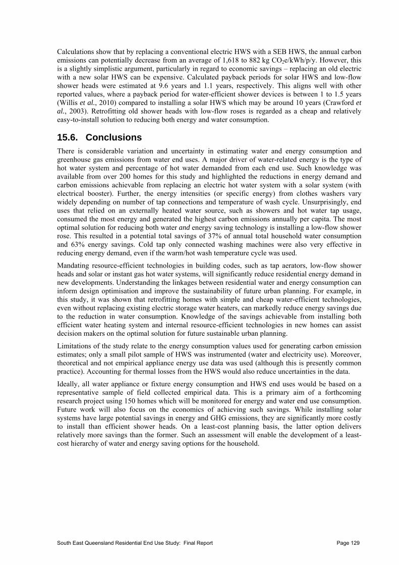
Calculations show that by replacing a conventional electric HWS with a SEB HWS, the annual carbon emissions can potentially decrease from an average of 1,618 to 882 kg CO2e/kWh/p/y. However, this is a slightly simplistic argument, particularly in regard to economic savings – replacing an old electric with a new solar HWS can be expensive. Calculated payback periods for solar HWS and low-flow shower heads were estimated at 9.6 years and 1.1 years, respectively. This aligns well with other reported values, where a payback period for water-efficient shower devices is between 1 to 1.5 years (Willis et al., 2010) compared to installing a solar HWS which may be around 10 years (Crawford et al., 2003). Retrofitting old shower heads with low-flow roses is regarded as a cheap and relatively easy-to-install solution to reducing both energy and water consumption.
15.6. Conclusions There is considerable variation and uncertainty in estimating water and energy consumption and greenhouse gas emissions from water end uses. A major driver of water-related energy is the type of hot water system and percentage of hot water demanded from each end use. Such knowledge was available from over 200 homes for this study and highlighted the reductions in energy demand and carbon emissions achievable from replacing an electric hot water system with a solar system (with electrical booster). Further, the energy intensities (or specific energy) from clothes washers vary widely depending on number of tap connections and temperature of wash cycle. Unsurprisingly, end uses that relied on an externally heated water source, such as showers and hot water tap usage, consumed the most energy and generated the highest carbon emissions annually per capita. The most optimal solution for reducing both water and energy saving technology is installing a low-flow shower rose. This resulted in a potential total savings of 37% of annual total household water consumption and 63% energy savings. Cold tap only connected washing machines were also very effective in reducing energy demand, even if the warm/hot wash temperature cycle was used.
Mandating resource-efficient technologies in building codes, such as tap aerators, low-flow shower heads and solar or instant gas hot water systems, will significantly reduce residential energy demand in new developments. Understanding the linkages between residential water and energy consumption can inform design optimisation and improve the sustainability of future urban planning. For example, in this study, it was shown that retrofitting homes with simple and cheap water-efficient technologies, even without replacing existing electric storage water heaters, can markedly reduce energy savings due to the reduction in water consumption. Knowledge of the savings achievable from installing both efficient water heating system and internal resource-efficient technologies in new homes can assist decision makers on the optimal solution for future sustainable urban planning.
Limitations of the study relate to the energy consumption values used for generating carbon emission estimates; only a small pilot sample of HWS was instrumented (water and electricity use). Moreover, theoretical and not empirical appliance energy use data was used (although this is presently common practice). Accounting for thermal losses from the HWS would also reduce uncertainties in the data.
Ideally, all water appliance or fixture energy consumption and HWS end uses would be based on a representative sample of field collected empirical data. This is a primary aim of a forthcoming research project using 150 homes which will be monitored for energy and water end use consumption. Future work will also focus on the economics of achieving such savings. While installing solar systems have large potential savings in energy and GHG emissions, they are significantly more costly to install than efficient shower heads. On a least-cost planning basis, the latter option delivers relatively more savings than the former. Such an assessment will enable the development of a least-cost hierarchy of water and energy saving options for the household.
South East Queensland Residential End Use Study: Final Report Page 129
16. CONCLUSIONS AND POLICY CONSIDERATIONS
This section highlights some results from the report that may be useful to inform future policy directions for demand management. The relatively low water consumption of 145 L/p/d reported for the initial winter 2010 analysis study confirms the anecdotal and government reporting of a shift in general water consumption post drought in SEQ. This may be partly a result of the prolonged water restrictions that have created a behavioural shift in SEQ consumers. Given that the sample was across four regions of varying levels of water restrictions in the recent past (e.g. severe for Brisbane and Ipswich, more relaxed for the Gold and Sunshine Coasts), the observed trend of generally lower water consumption is likely to be representative across SEQ. Subsequent summer 2010-11 and winter 2011 analysis revealed that average total water consumption remained below 145 L/p/d for SEQ. A number of key points from the report have been summarised below:
- End uses that are always high and that consistently contribute to peak hour and peak day demand are showers, clothes washers and taps. Sporadic irrigation events can sometimes be highly influential contributors to peak demand.
- Shower use is consistently high across all regions, contributing an average of around 30% of the total household consumption. There is a trend toward greater use amongst older, smaller households and younger, larger families. Water efficient showerheads will reduce total household water use substantially.
- Clothes washing consistently contributed 20% or more of total household water use. Elevated usage of clothes washers was generally associated with larger and younger families, and the older age brackets. This may be explained by the lower numbers of water efficient washing machines that were present in these older households. Conversely, large families with young children tended to have more efficient and updated models, therefore reducing the water demand for this end use.
- Tap use is the third highest water end use and is likely to go “unnoticed” due to the small volumes typically being used per each individual tap event. The cumulative and non-automated nature of tap use may be contributing to its high (19%) proportion of total consumption. Additionally, taps are readily accessible to young children and are often sources of leaks. Therefore, tap use may be an area to target with emphasis on the use of flow regulators and aerators, repairing faulty taps and increasing levels of awareness on the degree to which tap use contributes to total household water consumption.
- A correlation between toilet use and leak rate diurnal patterns suggests that this may be an area to target in reducing residential demand. The greatest associations between leak and toilets were in the Gold and Sunshine Coasts.
- Leaking toilets were more widespread than previously reported, however intervention programmes can be very effective at reducing these leaks as was shown in the summer and winter 2011 monitoring.
- There is still some degree of non-compliant irrigation between 10 am and 4 pm, particularly for homes in the Sunshine and Gold Coasts. This practice appears to have increased rather than decreased over the 18 month monitoring period, suggesting that the average resident is no longer as aware of the water restrictions in place under the Permanent Water Conservation Measures. Therefore, it is likely that a new/revised message is needed to increase the awareness of the current PWCM.
- Diurnal patterns revealed that peak hourly irrigation is occurring outside the restricted times of 10 am to 4 pm, although cumulatively, there is a large proportion of irrigation occurring within these hours. Comparisons of winter and summer irrigation patterns will elicit a greater understanding of these trends. Sunshine Coast and Gold Coast householders, who had a generally older demographic, were the least compliant in terms of irrigation times.
- The morning period (7-9 am) included the highest peak hour demand in all regions for the average day diurnal pattern curve. Showering and clothes washing contributed to approximately two thirds of this demand, indicating that policies targeting reductions in peak demand for capital efficiency purposes would need to consider these end uses.
South East Queensland Residential End Use Study: Final Report Page 130
- Further diurnal pattern analysis during summer periods will better reveal how irrigation contributes to peak hourly demand on the average day. Also, further analysis will seek to determine the maximum consumption day (including the peak hour) diurnal pattern curve (usually occurs in Christmas holiday period) to reveal the ratio of this particular maximum day peak hour to the average day peak hour. Such analysis could serve to help refine existing network models and thus pump and pipe infrastructure planning for a region.
- Reduced peak demand flow rates as a result of the mandated water-efficient technology and internally plumbed rainwater tanks in all new developments are likely to have substantial implications to water distribution networks.
- As a result of the likelihood of considerably lower peak flows in future developments, particularly where development codes mandate the installation of water efficient technology, it is recommended that future network modelling tasks completed by engineers incorporate real reductions in future peak demand. There is the potential for significant capital efficiency opportunities derived from the potential for smaller diameter pipe infrastructure in new developments as well as providing a basis for deferring an existing supply network’s inevitable future upgrade costs.
- Water efficient fittings for showers and taps are an excellent least-cost water demand management option for conserving water, confirming previous studies.
- With a combination of financial incentives for retrofitting water wise technology (i.e. low-flow shower roses, 4+ star rated washing machines) and revised building codes mandating such fixtures and appliances in new developments in Queensland, there will be an expected reduction in residential water demand. However, data presented in this report clearly illustrates the need for ongoing policy and water conservation initiatives to reduce shower consumption, which continues to represent around a third of average total household consumption.
- Changing to efficient washing machines and low-flow showerheads significantly reduces household water consumption. Diurnal patterns indicate that by encouraging a shift in clothes washer operation from morning to evening, like the existing habit for dishwashers, would substantially reduce the average morning peak demand.
- Families with young children are high water consumers on a household basis; this is a target area for sustained water conservation management. Single person households, while having a high per capita consumption, typically do not contribute to the peak day demand periods.
- Younger aged households were observed to use less water per capita and this may have some interesting implications for newer developments that are tending toward larger, younger families e.g. master planned communities.
- Although younger families may, in general, use less water per capita, data presented here demonstrates that targeting shower consumption, particularly in younger, larger families with teenagers may be a prudent focus for demand managers. Results from this report and elsewhere (e.g. Stewart et al., 2011) also suggest that a sustained targeting of shower consumption behaviour is required in high water use households, as behaviour, rather than technology, may dictate long term showering practices.
- The disparity between perceived and actual water use behaviour and the over- or underestimation of water use by householders demonstrates that there cannot be exclusive reliance on individual household attitudes and beliefs to reduce water consumption. Mandatory measures such as water restrictions or incentives such as clothes washing machine rebates are possibly more reliable in reducing residential demand.
- Characteristics of groups who overestimate their water use: o Lower incomes, less children, small household occupancies, less likely to have water
efficient technology. - Characteristics of groups who underestimate their water use:
o Higher incomes, larger families with young children, more water efficient technology, including low-flow shower roses and higher star rated washing machines.
- Frequent and high volume water end uses such as clothes washing, showering and tap use were associated with the incorrect estimations of household consumption.
- Heightened feedback to consumers on their households’ water consumption will improve their awareness and understanding of water use and help to encourage future water conservation behaviours.
South East Queensland Residential End Use Study: Final Report Page 131
South East Queensland Residential End Use Study: Final Report Page 132
- Clustered water flow rate intervals revealed that around 10% of flow is ≤ 100 L/hr, which is mainly contributed to leaks and internal tap use. Very low flow leaks are likely not to be registered by existing water meters.
- End uses associated with high flow rates (1,000 < 1,800 L/hr) included shower, clothes washing, external tap use, irrigation and uncommon water usage (e.g. service break leaks). These very high flow rates contributed to 10% of the total consumption.
- Results demonstrated that replacing an electric HWS with a solar HWS can achieve up to 43% reduction in energy consumption and carbon emissions.
- Retrofitting homes with simple and cheap water-efficient technologies, even without replacing existing electric HWS, can markedly reduce energy savings due to the reduction in water consumption.
- A number of different intervention scenarios aimed at shower end usage will be effective in reducing both water and energy demand. The most optimal solution is installing a low-flow shower rose, with potential total savings of 37% of annual total household water consumption and 63% energy savings. Reducing the temperature of the shower hot water from 40 to 37°C can also result in notable energy savings of about 13%.
- Front loading, single tap (cold) connected clothes washers can potentially reduce water and energy consumption by up to 27% and 87%, respectively.
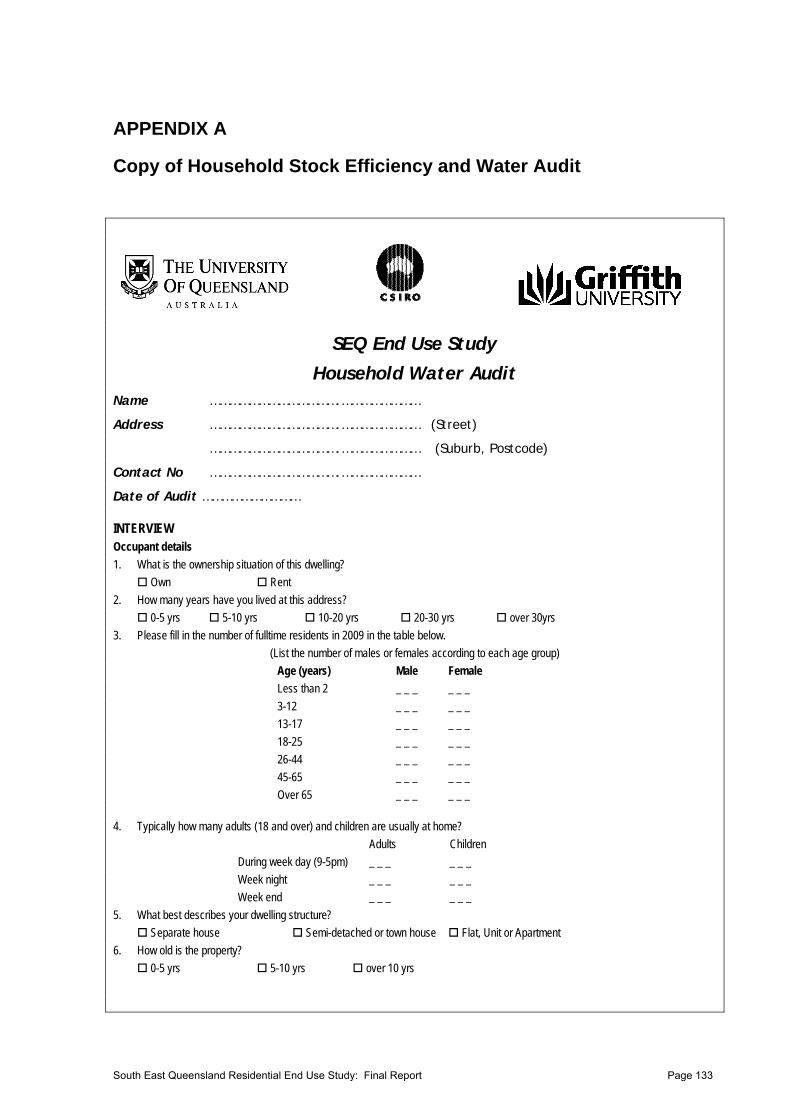
APPENDIX A
Copy of Household Stock Efficiency and Water Audit
SEQ End Use Study
Household Water Audit Name ………………………………….……………………
Address ………………………………….…………………… (Street)
………………………………….…………………… (Suburb, Postcode)
Contact No ………………………………….……………………
Date of Audit ………………………… INTERVIEW Occupant details
1. What is the ownership situation of this dwelling?
Own Rent
2. How many years have you lived at this address?
0-5 yrs 5-10 yrs 10-20 yrs 20-30 yrs over 30yrs
3. Please fill in the number of fulltime residents in 2009 in the table below.
(List the number of males or females according to each age group)
Age (years) Male Female
Less than 2 _ _ _ _ _ _
3-12 _ _ _ _ _ _
13-17 _ _ _ _ _ _
18-25 _ _ _ _ _ _
26-44 _ _ _ _ _ _
45-65 _ _ _ _ _ _
Over 65 _ _ _ _ _ _
4. Typically how many adults (18 and over) and children are usually at home?
Adults Children
During week day (9-5pm) _ _ _ _ _ _
Week night _ _ _ _ _ _
Week end _ _ _ _ _ _
5. What best describes your dwelling structure?
Separate house Semi-detached or town house Flat, Unit or Apartment
6. How old is the property?
0-5 yrs 5-10 yrs over 10 yrs
South East Queensland Residential End Use Study: Final Report Page 133
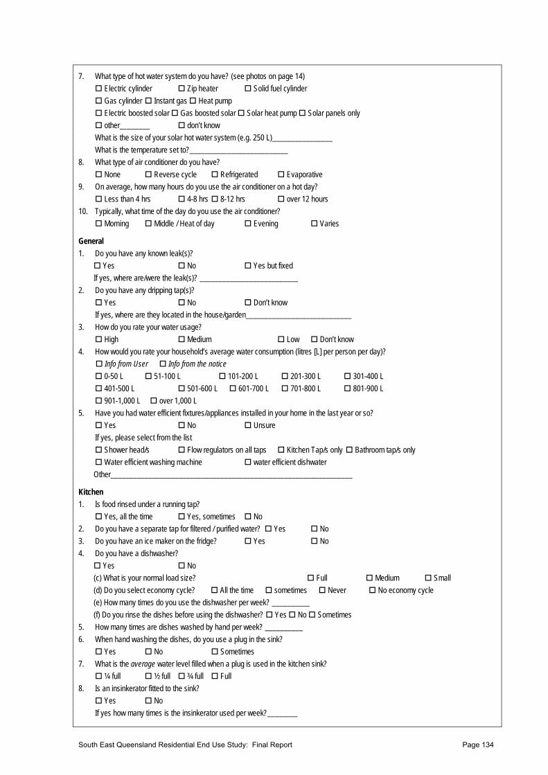
7. What type of hot water system do you have? (see photos on page 14)
Electric cylinder Zip heater Solid fuel cylinder
Gas cylinder Instant gas Heat pump
Electric boosted solar Gas boosted solar Solar heat pump Solar panels only
other________ don’t know
What is the size of your solar hot water system (e.g. 250 L)________________
What is the temperature set to?__________________________
8. What type of air conditioner do you have?
None Reverse cycle Refrigerated Evaporative
9. On average, how many hours do you use the air conditioner on a hot day?
Less than 4 hrs 4-8 hrs 8-12 hrs over 12 hours
10. Typically, what time of the day do you use the air conditioner?
Morning Middle / Heat of day Evening Varies
General
1. Do you have any known leak(s)?
Yes No Yes but fixed
If yes, where are/were the leak(s)? __________________________
2. Do you have any dripping tap(s)?
Yes No Don’t know
If yes, where are they located in the house/garden____________________________
3. How do you rate your water usage?
High Medium Low Don’t know
4. How would you rate your household’s average water consumption (litres [L] per person per day)?
Info from User Info from the notice
0-50 L 51-100 L 101-200 L 201-300 L 301-400 L
401-500 L 501-600 L 601-700 L 701-800 L 801-900 L
901-1,000 L over 1,000 L
5. Have you had water efficient fixtures/appliances installed in your home in the last year or so?
Yes No Unsure
If yes, please select from the list
Shower head/s Flow regulators on all taps Kitchen Tap/s only Bathroom tap/s only
Water efficient washing machine water efficient dishwater
Other________________________________________________________________
Kitchen
1. Is food rinsed under a running tap?
Yes, all the time Yes, sometimes No
2. Do you have a separate tap for filtered / purified water? Yes No
3. Do you have an ice maker on the fridge? Yes No
4. Do you have a dishwasher?
Yes No
(c) What is your normal load size? Full Medium Small
(d) Do you select economy cycle? All the time sometimes Never No economy cycle
(e) How many times do you use the dishwasher per week? __________
(f) Do you rinse the dishes before using the dishwasher? Yes No Sometimes
5. How many times are dishes washed by hand per week? __________
6. When hand washing the dishes, do you use a plug in the sink?
Yes No Sometimes
7. What is the average water level filled when a plug is used in the kitchen sink?
¼ full ½ full ¾ full Full
8. Is an insinkerator fitted to the sink?
Yes No
If yes how many times is the insinkerator used per week?________
South East Queensland Residential End Use Study: Final Report Page 134
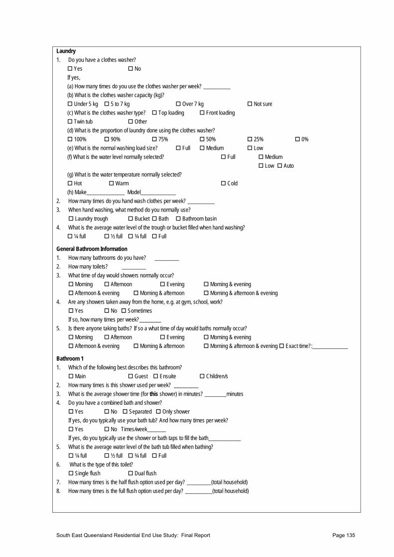
Laundry
1. Do you have a clothes washer?
Yes No
If yes,
(a) How many times do you use the clothes washer per week? __________
(b) What is the clothes washer capacity (kg)?
Under 5 kg 5 to 7 kg Over 7 kg Not sure
(c) What is the clothes washer type? Top loading Front loading
Twin tub Other
(d) What is the proportion of laundry done using the clothes washer?
100% 90% 75% 50% 25% 0%
(e) What is the normal washing load size? Full Medium Low
(f) What is the water level normally selected? Full Medium
Low Auto
(g) What is the water temperature normally selected?
Hot Warm Cold
(h) Make______________ Model_____________
2. How many times do you hand wash clothes per week? __________
3. When hand washing, what method do you normally use?
Laundry trough Bucket Bath Bathroom basin
4. What is the average water level of the trough or bucket filled when hand washing?
¼ full ½ full ¾ full Full
General Bathroom Information
1. How many bathrooms do you have? _________
2. How many toilets? _________
3. What time of day would showers normally occur?
Morning Afternoon Evening Morning & evening
Afternoon & evening Morning & afternoon Morning & afternoon & evening
4. Are any showers taken away from the home, e.g. at gym, school, work?
Yes No Sometimes
If so, how many times per week?________
5. Is there anyone taking baths? If so a what time of day would baths normally occur?
Morning Afternoon Evening Morning & evening
Afternoon & evening Morning & afternoon Morning & afternoon & evening Exact time?:_____________
Bathroom 1
1. Which of the following best describes this bathroom?
Main Guest Ensuite Children/s
2. How many times is this shower used per week? _________
3. What is the average shower time (for this shower) in minutes? ________minutes
4. Do you have a combined bath and shower?
Yes No Separated Only shower
If yes, do you typically use your bath tub? And how many times per week?
Yes No Times/week_______
If yes, do you typically use the shower or bath taps to fill the bath____________
5. What is the average water level of the bath tub filled when bathing?
¼ full ½ full ¾ full Full
6. What is the type of this toilet?
Single flush Dual flush
7. How many times is the half flush option used per day? _________(total household)
8. How many times is the full flush option used per day? __________(total household)
South East Queensland Residential End Use Study: Final Report Page 135
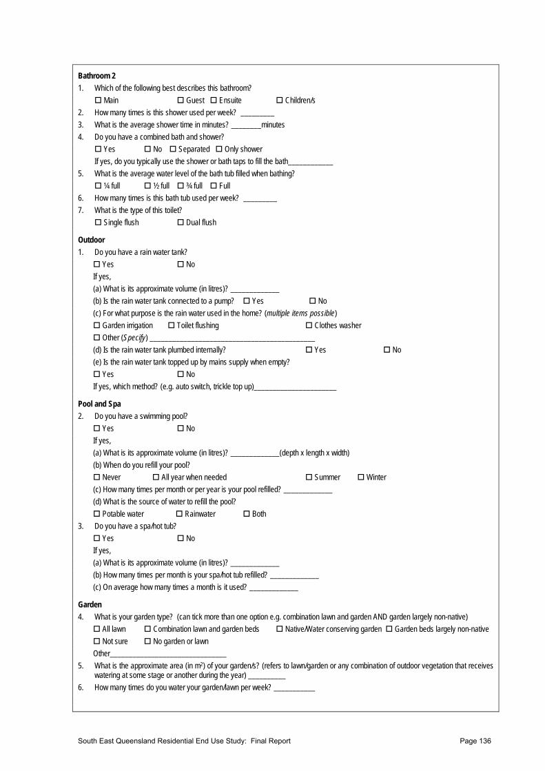
Bathroom 2
1. Which of the following best describes this bathroom?
Main Guest Ensuite Children/s
2. How many times is this shower used per week? _________
3. What is the average shower time in minutes? ________minutes
4. Do you have a combined bath and shower?
Yes No Separated Only shower
If yes, do you typically use the shower or bath taps to fill the bath____________
5. What is the average water level of the bath tub filled when bathing?
¼ full ½ full ¾ full Full
6. How many times is this bath tub used per week? _________
7. What is the type of this toilet?
Single flush Dual flush
Outdoor
1. Do you have a rain water tank?
Yes No
If yes,
(a) What is its approximate volume (in litres)? _____________
(b) Is the rain water tank connected to a pump? Yes No
(c) For what purpose is the rain water used in the home? (multiple items possible)
Garden irrigation Toilet flushing Clothes washer
Other (Specify) ____________________________________________
(d) Is the rain water tank plumbed internally? Yes No
(e) Is the rain water tank topped up by mains supply when empty?
Yes No
If yes, which method? (e.g. auto switch, trickle top up)______________________
Pool and Spa
2. Do you have a swimming pool?
Yes No
If yes,
(a) What is its approximate volume (in litres)? _____________(depth x length x width)
(b) When do you refill your pool?
Never All year when needed Summer Winter
(c) How many times per month or per year is your pool refilled? _____________
(d) What is the source of water to refill the pool?
Potable water Rainwater Both
3. Do you have a spa/hot tub?
Yes No
If yes,
(a) What is its approximate volume (in litres)? _____________
(b) How many times per month is your spa/hot tub refilled? _____________
(c) On average how many times a month is it used? _____________
Garden
4. What is your garden type? (can tick more than one option e.g. combination lawn and garden AND garden largely non-native)
All lawn Combination lawn and garden beds Native/Water conserving garden Garden beds largely non-native
Not sure No garden or lawn
Other_______________________________
5. What is the approximate area (in m2) of your garden/s? (refers to lawn/garden or any combination of outdoor vegetation that receives watering at some stage or another during the year) __________
6. How many times do you water your garden/lawn per week? ___________
South East Queensland Residential End Use Study: Final Report Page 136
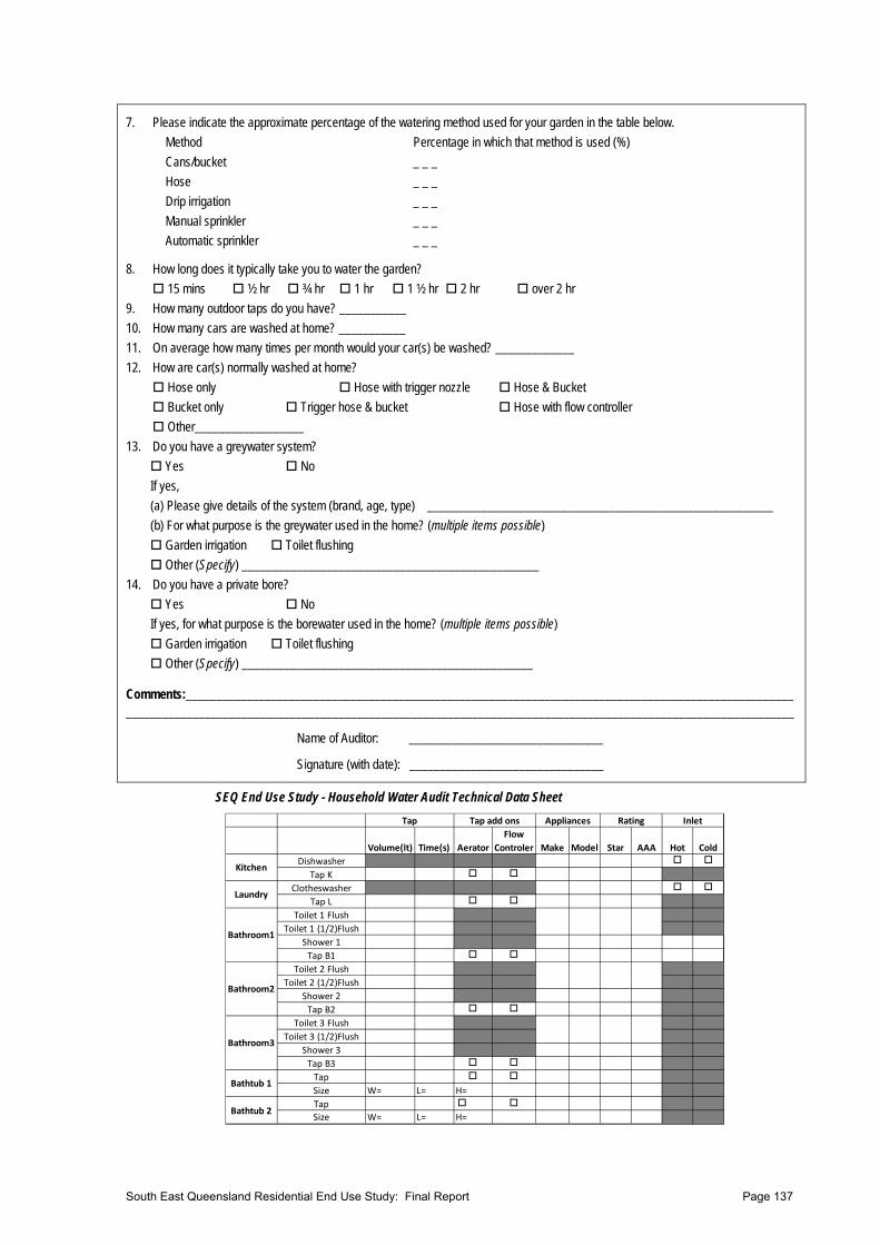
7. Please indicate the approximate percentage of the watering method used for your garden in the table below.
Method Percentage in which that method is used (%)
Cans/bucket _ _ _
Hose _ _ _
Drip irrigation _ _ _
Manual sprinkler _ _ _
Automatic sprinkler _ _ _
8. How long does it typically take you to water the garden?
15 mins ½ hr ¾ hr 1 hr 1 ½ hr 2 hr over 2 hr
9. How many outdoor taps do you have? ___________
10. How many cars are washed at home? ___________
11. On average how many times per month would your car(s) be washed? _____________
12. How are car(s) normally washed at home?
Hose only Hose with trigger nozzle Hose & Bucket
Bucket only Trigger hose & bucket Hose with flow controller
Other__________________
13. Do you have a greywater system?
Yes No
If yes,
(a) Please give details of the system (brand, age, type) _________________________________________________________
(b) For what purpose is the greywater used in the home? (multiple items possible)
Garden irrigation Toilet flushing
Other (Specify) _________________________________________________
14. Do you have a private bore?
Yes No
If yes, for what purpose is the borewater used in the home? (multiple items possible)
Garden irrigation Toilet flushing
Other (Specify) ________________________________________________
Comments:__________________________________________________________________________________________________________________________________________________________________________________________________________________
Name of Auditor: ________________________________
Signature (with date): ________________________________
SEQ End Use Study - Household Water Audit Technical Data Sheet
Volume(lt) Time(s) Aerator
Flow
Controler Make Model Star AAA Hot Cold
Dishwasher
Tap K
Clotheswasher
Tap L
Toilet 1 Flush
Toilet 1 (1/2)Flush
Shower 1
Tap B1
Toilet 2 Flush
Toilet 2 (1/2)Flush
Shower 2
Tap B2
Toilet 3 Flush
Toilet 3 (1/2)Flush
Shower 3
Tap B3
Tap
Size W= L= H=
Tap
Size W= L= H=
InletAppliances Rating
Bathroom3
Bathroom2
Bathtub 1
Bathtub 2
Tap Tap add ons
Bathroom1
Laundry
Kitchen
South East Queensland Residential End Use Study: Final Report Page 137
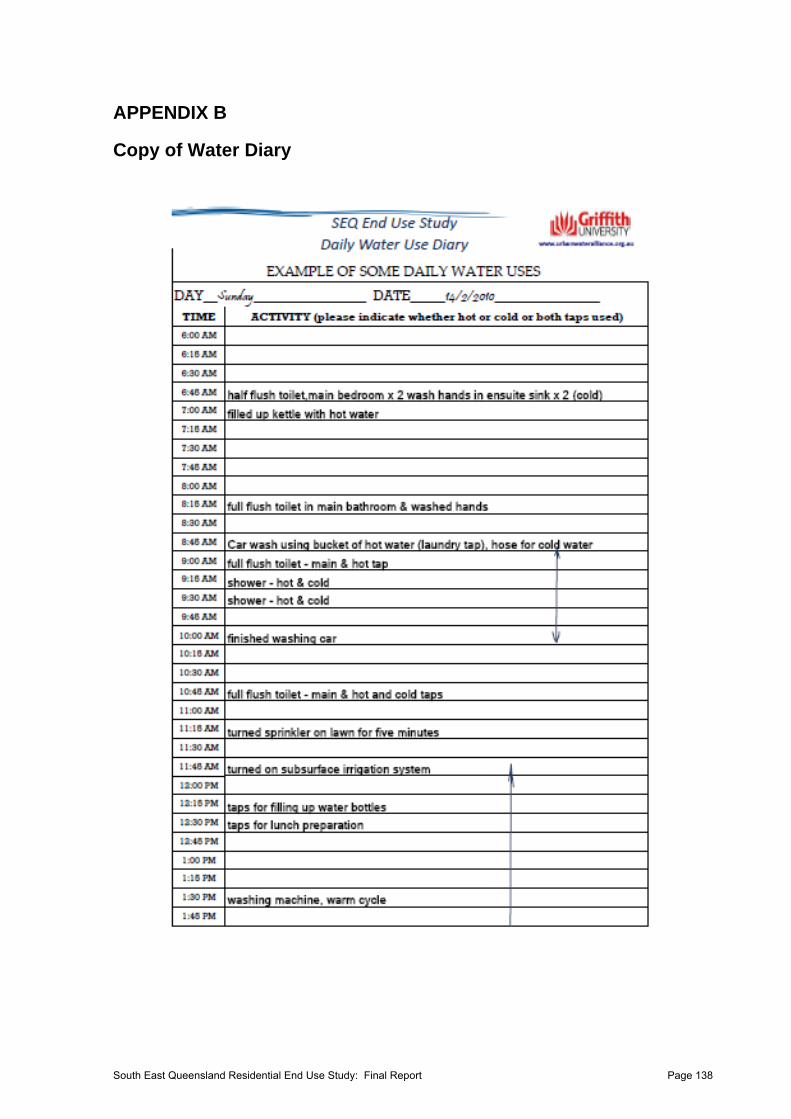
APPENDIX B
Copy of Water Diary
South East Queensland Residential End Use Study: Final Report Page 138

APPENDIX C
SEQREUS Winter 2010 End Use Frequency Distributions
South East Queensland Residential End Use Study: Final Report Page 139
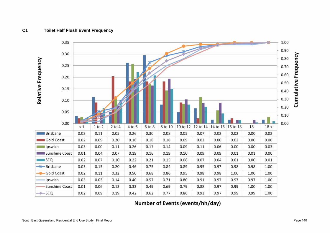
C1 Toilet Half Flush Event Frequency
South East Queensland Residential End Use Study: Final Report Page 140
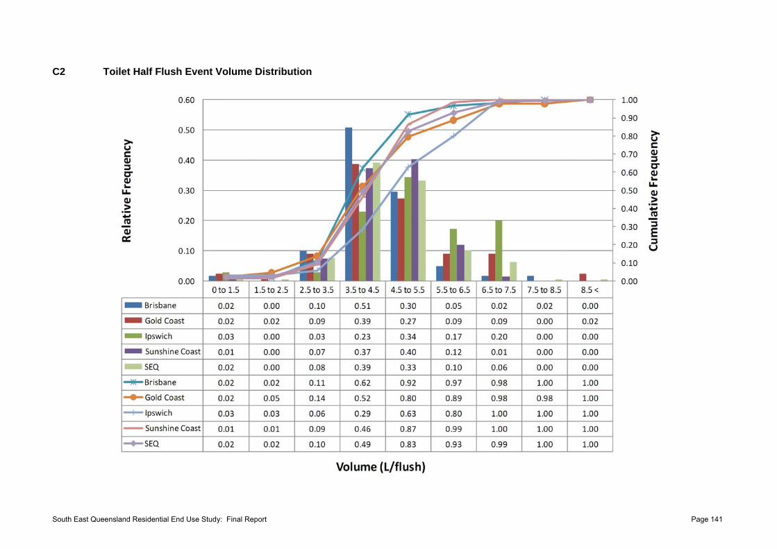
C2 Toilet Half Flush Event Volume Distribution
South East Queensland Residential End Use Study: Final Report Page 141
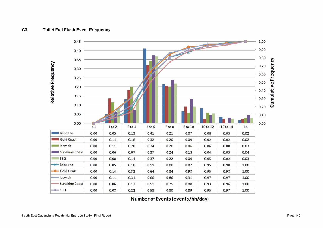
C3 Toilet Full Flush Event Frequency
South East Queensland Residential End Use Study: Final Report Page 142
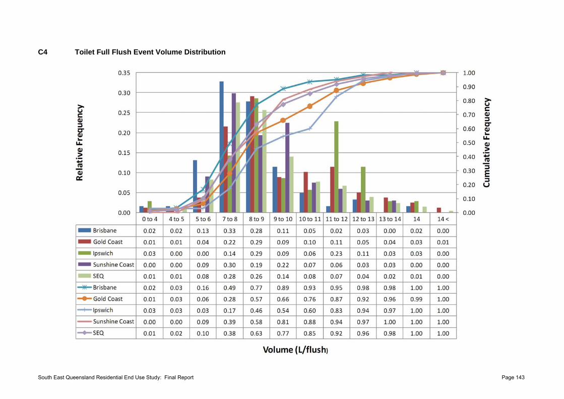
C4 Toilet Full Flush Event Volume Distribution
South East Queensland Residential End Use Study: Final Report Page 143
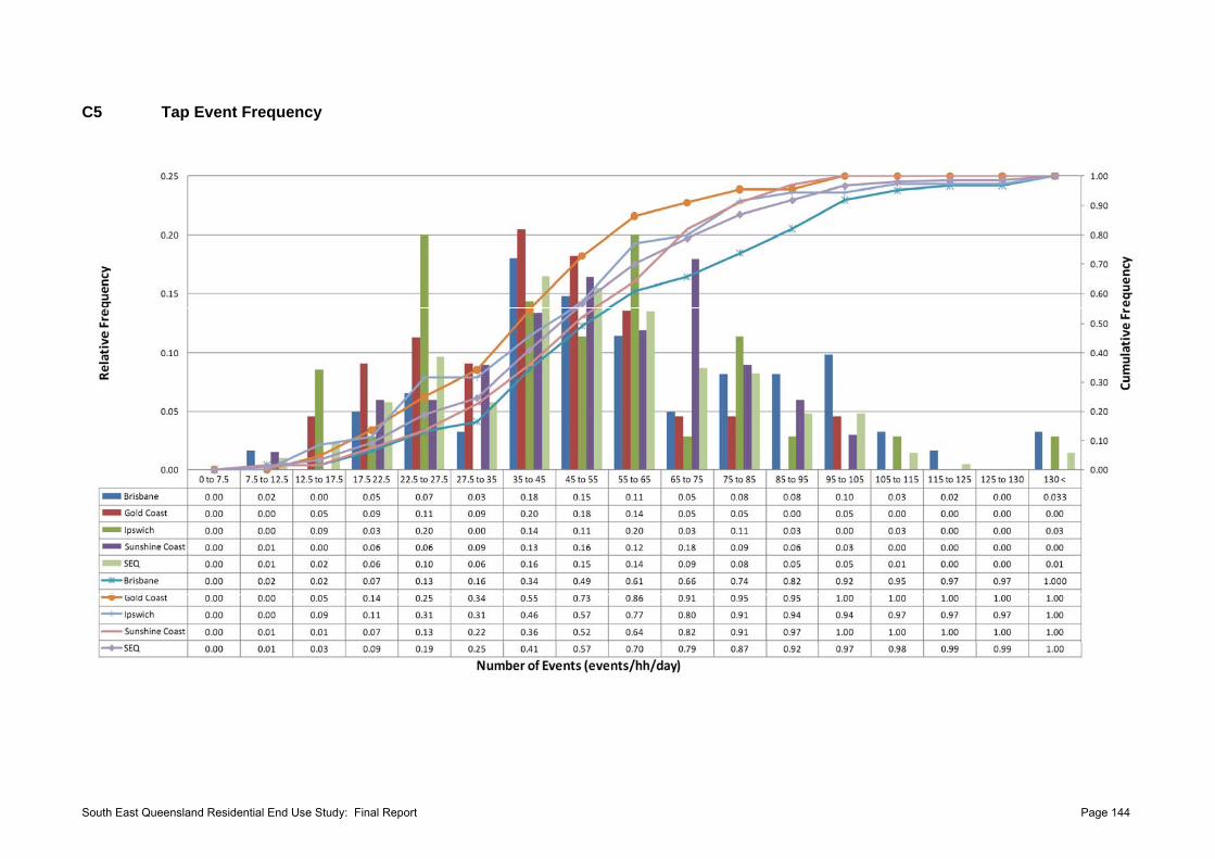
C5 Tap Event Frequency
South East Queensland Residential End Use Study: Final Report Page 144
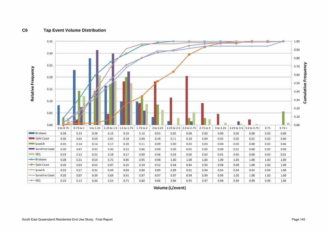
C6 Tap Event Volume Distribution
South East Queensland Residential End Use Study: Final Report Page 145
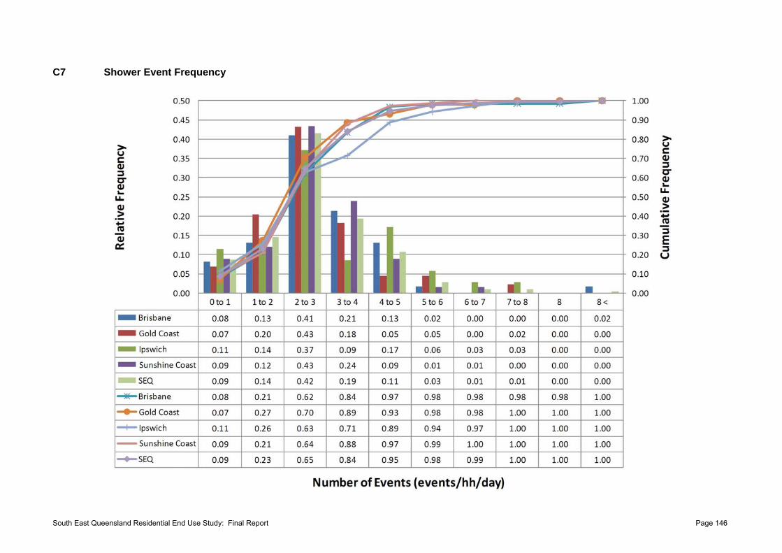
C7 Shower Event Frequency
South East Queensland Residential End Use Study: Final Report Page 146
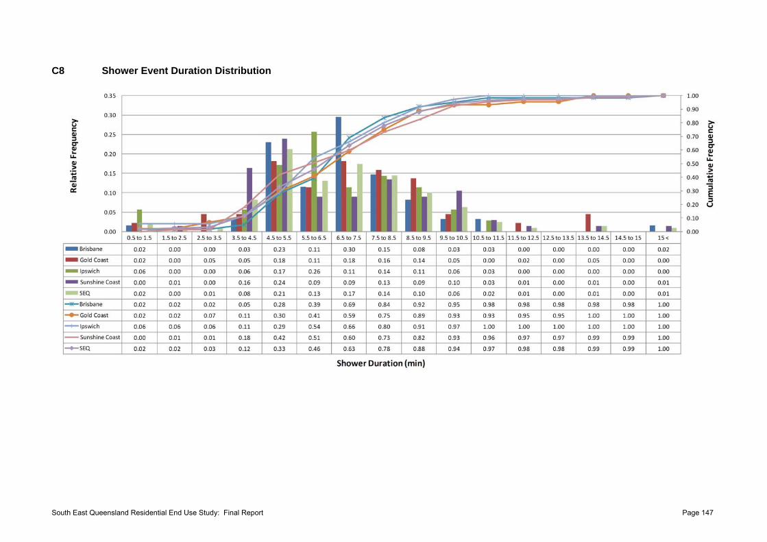
C8 Shower Event Duration Distribution
South East Queensland Residential End Use Study: Final Report Page 147
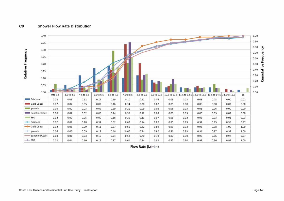
C9 Shower Flow Rate Distribution
South East Queensland Residential End Use Study: Final Report Page 148
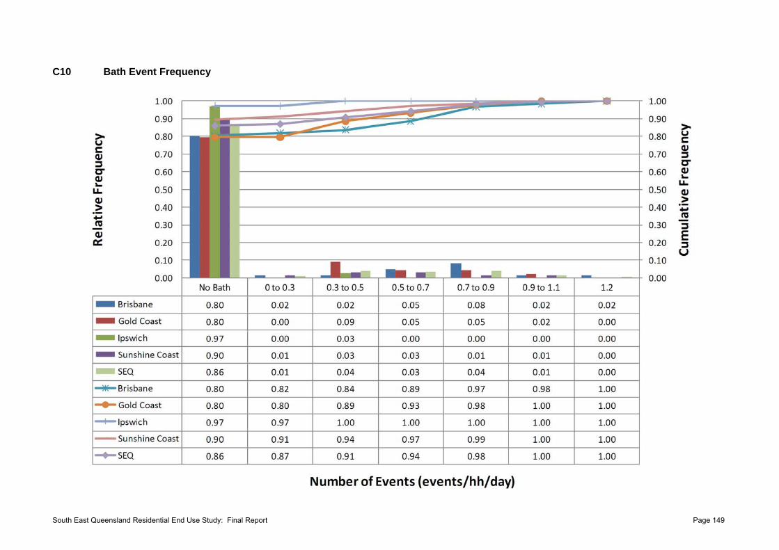
C10 Bath Event Frequency
South East Queensland Residential End Use Study: Final Report Page 149
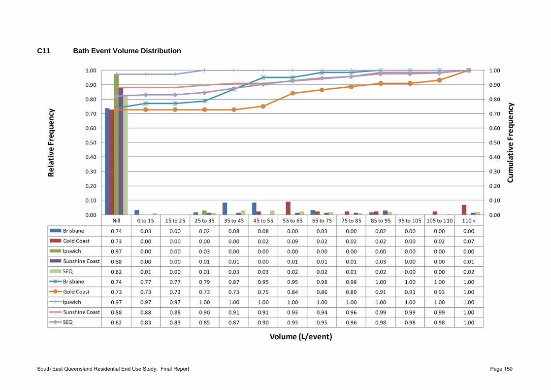
C11 Bath Event Volume Distribution
South East Queensland Residential End Use Study: Final Report Page 150

C12 Bath Event Filling Rate Distribution
South East Queensland Residential End Use Study: Final Report Page 151
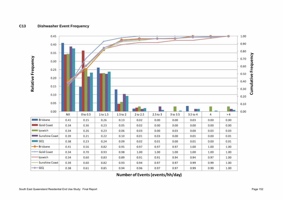
C13 Dishwasher Event Frequency
South East Queensland Residential End Use Study: Final Report Page 152
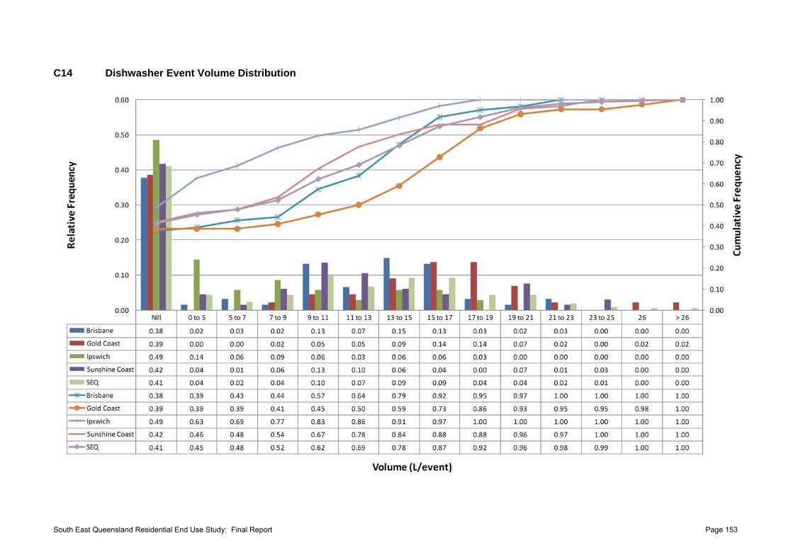
C14 Dishwasher Event Volume Distribution
South East Queensland Residential End Use Study: Final Report Page 153
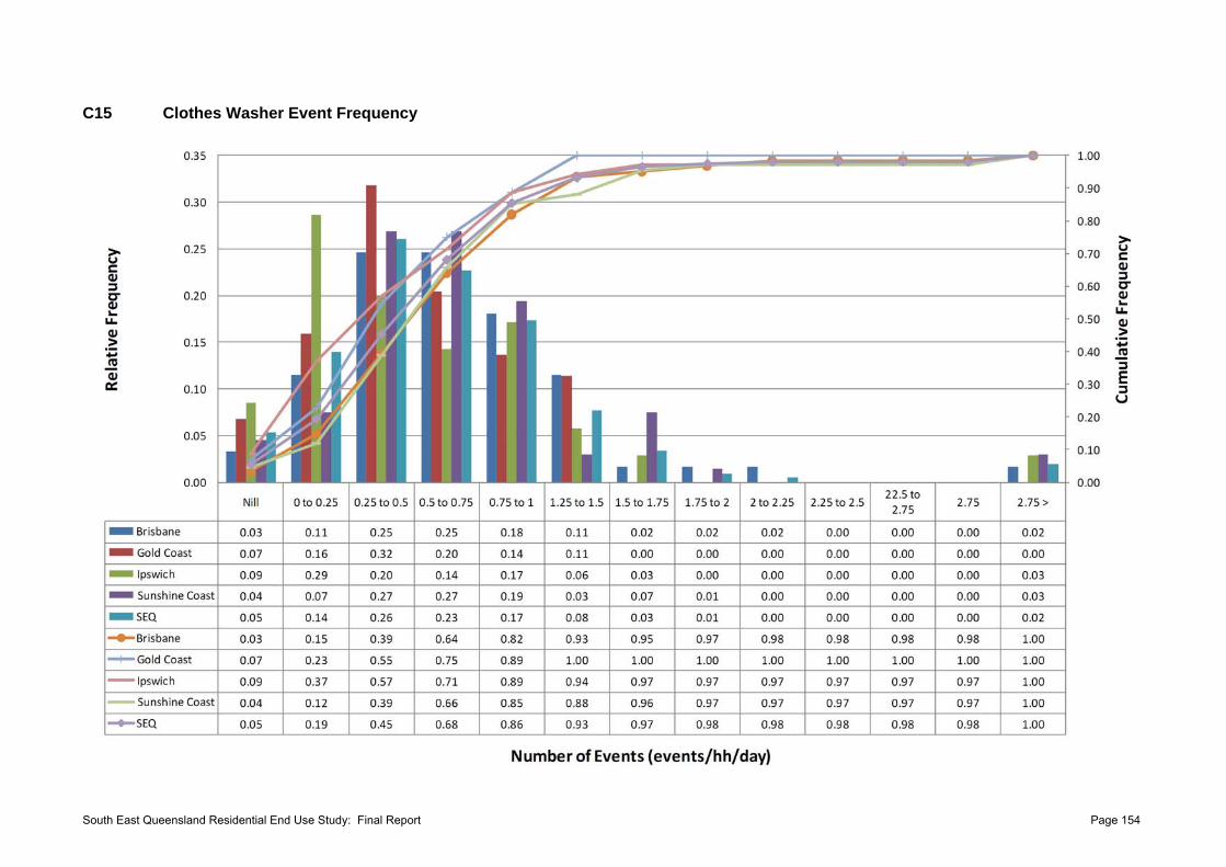
C15 Clothes Washer Event Frequency
South East Queensland Residential End Use Study: Final Report Page 154
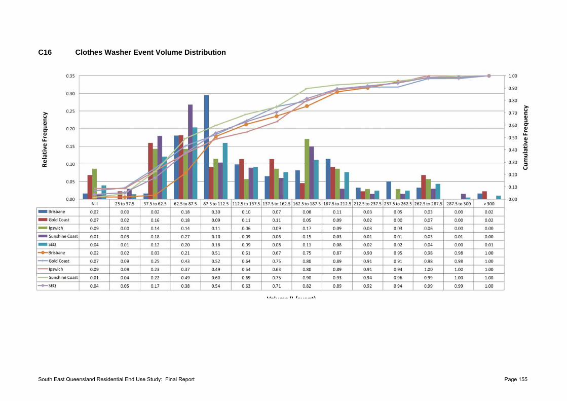
C16 Clothes Washer Event Volume Distribution
South East Queensland Residential End Use Study: Final Report Page 155
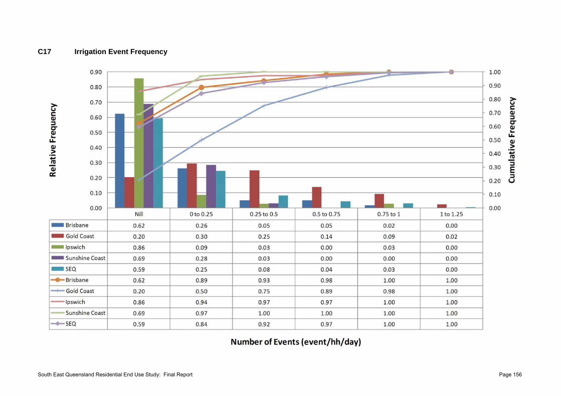
C17 Irrigation Event Frequency
South East Queensland Residential End Use Study: Final Report Page 156
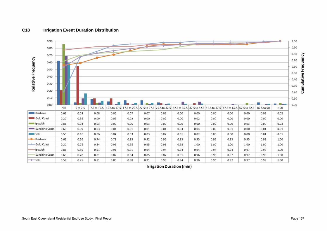
C18 Irrigation Event Duration Distribution
South East Queensland Residential End Use Study: Final Report Page 157
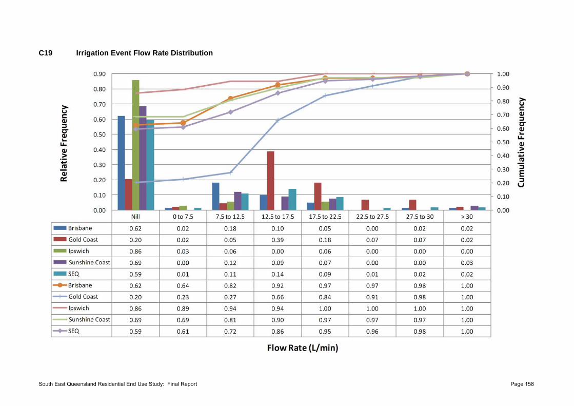
C19 Irrigation Event Flow Rate Distribution
South East Queensland Residential End Use Study: Final Report Page 158
REFERENCES
ABC News (2011) Brisbane floods: before and after. In ABC News, 17 January 2011, http://www.abc.net.au/news/infographics/qldfloods/beforeafter.htm. Accessed November 17th, 2011.
Anker-Nilssen, P., 2003. Household energy use and the environment--a conflicting issue. Applied Energy, 76(1-3), 189-196.
Aquacraft (2010). Trace Wizard® software version 4.1. 1995-2010 Aquacraft, Inc. Boulder, CO, USA. http://www.aquacraft.com/
Arbués, F., García-Valiñas, M.A. and Martínez-Espiñeira, R. (2003). Estimation of residential water demand: a state-of-the-art review. Journal of Socio-Economics 32: 81-102.
Arbues, F., Villanua, I. and Barberan, R., 2010. Household size and residential water demand: an empirical approach. The Australian Journal of Agricultural and Resource Economics 54, 61-80.
Australian Government (2010a). National Greenhouse Accounts (NGA) Factors, prepared by the Department of Climate Change and Energy Efficiency, July 2010.
Australian Government (2010b) Water efficiency labeling and standards (WELS) scheme. Commonwealth of Australia website: http://www.waterrating.gov.au/products/index.html. Accessed 10th October 2011.
Australian Government (2010c) E3 Equipment, Energy, Efficiency. Commonwealth of Australia website: http://www.energyrating.gov.au/compare-products/ Accessed 10th October 2011.
Barrett, G. and Wallace, M. (2009). Characteristics of Australian urban residential water users: implications for water demand management and whole of the system water accounting framework. Water Policy, 11 413:426.
Baruch, Y. and Brooks, C. (2008) Survey response rate levels in and trends in organizational research. Human Relations 61(8), 1139-1160.
Beal, C., Gardner, T., Sharma, A. Barton, R. and Chong, M. (2011c). A Desktop Analysis of Potable Water Savings from Internally Plumbed Rainwater Tanks in South East Qld. Urban Water Security Research Alliance Technical Report No. 26. http://www.urbanwateralliance.org.au/publications/ UWSRA-tr26.pdf
Beal, C., Stewart, R., Huang, T., Rey, E., (2011b). SEQ residential end use study. Australian Water Association Journal, 38(1), 80-84.
Beal, C.D., Stewart, R.A. and Bertone, E. (2012) Evaluating the energy and carbon reductions resulting from resource-efficient household stock. Energy and Buildings, in press, DOI 10.1016/j.enbuild.2012.08.004.
Beal, C.D., Stewart, R.A., Fielding, K. A novel mixed method smart metering approach to reconciling differences between perceived and actual residential end use water consumption, Journal of Cleaner Production (2011a), doi:10.1016/j.jclepro.2011.09.007.
Beal, C.D., Stewart, R.A., Talebpour, R., Huang, A. and Rey, E. (2010). South East Queensland residential end use study: Pilot study of Gold Coast households. Technical Report for Urban Water Security Research Alliance. Griffith University and Smart Water Research Centre, September, 2010.
Beal, C.D., Stewart, R.A., (2012) Identifying residential water end uses underpinning peak day and hour demand. Journal of Water Resources Planning and Management (under review).
Blokker, E., Vreeburg, J. and van Dijk, J. (2010). Simulating residential water demand with a stochastic end-use model. Journal of Water Resources, Planning and Management 136(1), 19-26.
Carragher, BJ., Stewart, RA. and Beal, CD., (2012) Quantifying the influence of residential water appliance efficiency on average day diurnal demand patterns at an end use level: A precursor to optimised water service infrastructure planning. Resource Conservation and Recycling, 62, 81-90.
Chang, H., Parandvash, G. and Shandas, V., 2010. Spatial variations of single-family residential water consumption in Portland, Oregon. Urban Geography 31, 953-972.
Cheng, C.-L. (2002) Study of the inter-relationship between water use and energy conservation for a building. Energy and Buildings 34, 261-266.
Chu, J., Wang, C., Chen, J. and Wang, H. (2009) Agent-based residential water use behavior simulation and policy implications: a case study in Beijing City. Water Resources Management 23, 3267-3295.
Clarke, A., Grant, N. and Thornton, J. (2009) Quantifying the energy and carbon effects of water savings, Full technical report for Environment Agency and Energy Savings Trust prepared by Elemental Solutions, April 2009, UK.
Cole, G and Stewart, R.A., (2012) Smart meter enabled disaggregation of urban peak water demand: precursor to effective urban water planning. Urban Water Journal, under review.
South East Queensland Residential End Use Study: Final Report Page 159
Corral-Verdugo, V., Bechtel, R. and Fraijo-Sing, B. (2002). Environmental beliefs and water conservation: an empirical study. Environmental Psychology, 23:247-257.
Corral-Verdugo, V., Frías-Armenta, M., 2006. Personal normative beliefs, antisocial behavior, and residential water conservation. Environment and Behavior 38(3), 406-421
DCCEE (2011) Department of Climate Change and Energy Efficiency – National Greenhouse Accounts (NGA) Factors – July 2011. Australian Government website http://www.climatechange.gov.au/~/media/publications/greenhouse-acctg/national-greenhouse-factors-july-2010-pdf. Accessed 10 September 2011.
DeOreo, W., Heaney, J. and Mayer, P. (1996). Flow trace analysis to assess water use. American Water Works Association Journal 88(1), 79-90.
DERM (2007). Chapter 5: Demand/flow and projections. Planning Guidelines for Water Supply and Sewerage, Department of Environment and Resource Management. June 2007 revision.
DIP (2007) Queensland Development Code. Queensland Government. January 2007. DIP (2009). South East Queensland Regional Plan 2009-2031. Department of Infrastructure and Planning,
Queensland Government. September 2009. Dolnicar, S., Hurlimann, A., 2010. Australian water conservation behaviours and attitudes [online].
Australian Journal of Water Resources, 14, 43-53. Domènech, L., Saurí, D., 2011. A comparative appraisal of the use of rainwater harvesting in single and
multi-family buildings of the Metropolitan Area of Barcelona (Spain): social experience, drinking water savings and economic costs. Journal of Cleaner Production 19, 598-608.
Druckman, A., Sinclair, P. and Jackson, T., 2008. A geographically and socio-economically disaggregated local household consumption model for the UK. Journal of Cleaner Production 16, 870-880.
England, P. (2009 ) Managing urban water in Australia: the planned and the unplanned Management of Environmental Quality: An International Journal 20(5), 592-608.
Farrelly, M., Brown, R., 2011. Rethinking urban water management: Experimentation as a way forward? Global Environmental Change 847, dio:10.1016/j.gloenvcha.2011.1001.1007.
Fidar, A., Memon, F. and Butler, D. (2010). Environmental implications of water efficient microcomponents in residential buildings. Science of the Total Environment, 408, 5828-5835.
Fielding, K., Spinks, A., Russell, S. and Mankad, A. (2011) Predictors of Household Water Use in South East Queensland, in Science Forum and Stakeholder Engagement: Building Linkages, Collaboration and Science Quality, (eds) D.K., Begbie and S.L., Wakem, Urban Water Security Research Alliance, September 2011, Brisbane, Queensland, pp 25.
Fielding, K., Spinks, A., Russell, S., MCCRea, R, Stewart, R.A., Gardner, J. An experimental test of voluntary strategies to promote urban water demand management. Under review, 2012.
Gardiner, A. (2009) Domestic rainwater tanks: usage and maintenance patterns in South East Queensland. Australian Water Association Journal 36(1), 74-77.
Gardner, T. and Vieritz, A. (2010) The role of rainwater tanks in Australia in the twenty first century. Architectural Science Review 53(1), 107-125.
Gato, S., Jayasuriya, N. and Roberts, P. (2007) Temperature and rainfall thresholds for base use urban water demand modelling. Journal of Hydrology 337(3-4), 364-376.
Gato-Trinidad, S., Jayasuriya, N. and Roberts, P. (2011) Understanding urban residential end uses of water. Water Science and Technology 64(1), 36-42.
GHD (2009). Desired Standards of Service Review 2008 Final Report Rev 3. 178/07/01_GHD-10. October, 2009.
Gilg, A. and Barr, S. (2006). Behavioural attitudes towards water saving? Evidence from a study of environmental actions. Ecological Economics, 57: 400-414.
Giurco, D., Carrard, N., McFallan, S., Nalbantoglu, M., Inman, M., Thornton, N. and White, S. (2008). Residential end-use measurement Guidebook: a guide to study design, sampling and technology. Prepared by the Institute for Sustainable Futures, UTS and CSIRO for the Smart Water Fund, Victoria.
Gleick P.H., Adams R.M., Amasino R.M., Anders E., Anderson D.J., Anderson W.W., Anselin L.E., et al. (2010). Climate change and the integrity of science. Science 328:689-690.
Gold Coast Water (2010). May Monthly Summary report – Water Supplied. Gold Coast Water and Gold Coast City Council, June, 2010.
Golden, J., Subramaniana, V., Irizarria, G., Whitec, P. and Meierd, F. (2010) Energy and carbon impact from residential laundry in the United States. Journal of Integrative Environmental Sciences 7(1), 53-73.
South East Queensland Residential End Use Study: Final Report Page 160
Gregory, G., Di Leo, M., 2003. Repeated behavior and environmental psychology: the role of personal involvement and habit formation in explaining water consumption. Applied Social Psychology 33(6), 1261-1296.
Hamilton, L., 1985. Self-reported and actual savings in a water conservation campaign. Environment and Behavior 17(3), 315-326.
Heinrich, M. (2007). Water End Use and Efficiency Project (WEEP) - Final Report. BRANZ Study Report 159, Branz, Judgeford, New Zealand.
Hoffman, M., Worthington, A. and Higgs, H. (2006). Urban water demand with fixed volumetric charging in a large municipality: the case of Brisbane, Australia. The Australian Journal of Agriculture and Resource Economics 50:347-359. http://www.waterrating.gov.au/products/index.html. Accessed November 24th, 2011.
Inman, D. and Jeffrey, P. (2006). A review of residential water conservation tool performance and influences on implementation effectiveness. Urban Water Journal, Vol 3:3, pp. 127-143.
Jacobs, H. and Haarhoff, J. (2004) Structure and data requirements of an end-use model or residential water demand and return flow. Water SA 30(3), 293-304.
Jones, N., Evangelinos, K., Gaganis, P. and Polyzou, E., 2010. Citizen's perceptions on water conservation policies and the role of social capital. Water Resources Management 25, 509-522.
Jorgensen, B., Graymore, M. and O'Toole, K., 2009. Household water use behavior: an integrated model. Journal of Environmental Management 91, 227-236.
Juárez-Nájera, M., Rivera-Martinez, J., Hafkamp, W., 2010. An explorative socio-physcological model for determining sustainable behavior: Pilot study in Germany and Mexican Universities. Journal of Cleaner Production 18, 686-694.
Kantola, S.J., Syme, G.J., Campbell, N.A., 1984. Cognitive dissonance and energy conservation. Journal of Applied Psychology 69(3), 416-421.
Kennedy, A., 2010. Using Community-Based Social Marketing Techniques to Enhance Environmental Regulation. Sustainability, 2(4), 1138-1160
Kenney, D.S., Goemans, C., Klein, R.A., Lowrey, J. and Reidy, K. (2008). Residential water demand management: lessons from Aurora, Colorado. Journal of the American Water resources Association, 44 (1):192-207.
Kenway, S., Priestley, A., Cook, S., Seo, S., Inman, M., Gregory, A. and Hall, M. (2008) Energy use in the provision and consumption of urban water in Australia and New Zealand, CSIRO:Water for a Healthy Country National Research Flagship.
Kenway, S.J., Lant, P., Preistly, T., Daniels, P., (2011) The connection between water and energy in cities. Water Science and Technology, 63, 1983-1990.
Keselman, H., Huberty, C., Lix, L., Olejnik, S., Cribbie, R., Donahue, B., Kowalchuk, R., Lowman, L., Petoskey, M., Keselman, J. and Levin, J., 1998. Statistical practices of educational researchers: an analysis of their ANOVA, MANOVA, and ANCOVA analyses. Review of Educational Research 68(3), 350-386.
Koomey, J., Dunham, C. and Lutz, J. (1995) The effect of efficient standards on the water use and water-heating energy use in the U.S: A detailed end-use treatment. Energy 20(7), 627-635.
Kowalski, M. and Marshallsay, D. (2005) Using measured microcomponent data to model the impact of water conservation strategies on the diurnal consumption profile. Water Science and Technology:Water Supply 5(3-4), 145-150.
Kraus, S.J., 1995. Attitudes and the prediction of behaviour: A meta-analysis of the empirical literature. Personal and Social Psychology Bulletin 2: 58-75
Lee, M., Tansel, B. and Balbin, M. (2011) Influence of residential water use efficiency measures on household water demand: A four year longitudinal study. Resources, Conservation and Recycling 56(1), 1-6.
Lenzen, M. and Peters, G.M. (2010) How City Dwellers Affect Their Resource Hinterland. Journal of Industrial Ecology 14(1), 73-90.
Loh, M. and Coghlan, P. (2003). Domestic water use study in Perth, Western Australia 1998 to 2000. Water Corporation of Western Australia.
Lynn, P. (2001) The impact of incentives on response rates to personal interview surveys: Role and perceptions of interviewers. international Journal of Public Opinion Research 13(3), 326-336.
Maas, C. (2009) Greenhouse gas energy co-benefits of water conservation, POLIS Research Report 09-01, March 2009
Makki, A., Stewart, R. and Beal, C. (2011) Revealing the determinants of shower water end use consumption: enabling better targeted urban water conservation strategies. Journal of Cleaner Production doi:10.1016/j.jclepro.2011.08.007.
South East Queensland Residential End Use Study: Final Report Page 161
Mayer, P., DeOreo, W., Towler, E., Martien, L. and Lewis, D. (2004) Tampa Water Department Residential water conservation study. The impacts of high efficiency plumbing fixture retrofits in single family homes, Tampa Water Department and The United States Environmental Protection Agency.
Mayer, P.W. and DeOreo, W.B. (1999). Residential End Uses of Water, Aquacraft, Inc. Water Engineering and Management, Boulder, CO.
Millock, K., Nauges, C., 2010. Household adoption of water-efficient equipment: the role of socio-economic factors, environmental attitudes and policy. Environmental Resource Economics, 46, 539-565.
MWH (2007). Regional water needs and integrated urban water management opportunities report. Report 4 of the SEQRWSSS IUWMA Taskgroup, MWA-01
Nieswiadomy, M., 1992. Estimating urban residential water demand: effects of price structure, conservation, and education. Water Resources Research 28(3), 609-615.
O’Toole, J., Sinclair, M. and Leder, K. (2009). Collecting household water usage data; telephone questionnaire or diary? BMC Medical Research Methodology, 9:72-83.
Olmstead, S., Stavins, R., 2009. Comparing price and nonprice approaches to urban water conservation. Water Resources Research, 45(W04301), doi:10.1029/2008WR007227.
Pachauri, S. (2004) An analysis of cross-sectional variations in total household energy requirements in India using micro survey data. Energy 32, 1723-1735.
Pakula, C. and Stamminger, R. (2010) Electricity and water consumption for laundry washing by washing machine worldwide. Energy Efficiency 3, 365-382.
QWC (2010a). South East Queensland Water Strategy, July 2010, The State of Queensland (Queensland Water Commission).
QWC (2010b). Queensland Water Commission website Media Release for 25th June 2010 http://www.qwc.qld.gov.au/tiki-read_article.php?articleId=410, accessed August 16th 2010.
Renwick, M., Archibald, S., 1998. Demand side management policies for residential water use: who bears the conservation burden? Land Economics 74(3), 343-359.
Roberts, P. (2005). Yarra Valley Water 2004 residential end use measurement study. Final report, June 2004.
Russell, S. and Fielding, K. (2010). Water demand management research: A psychological perspective, Water Resources Research, 46, W05302, doi10.1029/2009WR008408.
Sivakumaran, S. and Aramaki, T. (2010). "Estimation of household water end use in Trincomalee, Sri Lanka." Water International 35(1): 94-99.
Solomon, S., Qin, D., Manning, M., Chen, Z., Marquis, M., Averyt, K., Tignor, M. and HL, M. (eds) (2007) Contribution of Working Group I to the Fourth Assessment Report of the Intergovernmental Panel on Climate Change, 2007, Cambridge University Press, Cambridge, United Kingdom and New York, NY, USA.
Spinks, A., Fielding, K., Russell, S., Mankad, A., Price, J., (forthcoming). Water demand management study: Baseline survey of household water use (Part A). Urban Water Security Research Alliance.
Stamminger, R. (2011) Modelling resource consumption for laundry and dish treatment in individual households for various consumer segments. Energy Efficiency 4(4), 559-569.
Stewart, R., Willis, R., Panuwatwanich, K. and Sahin, O. (2011) Showering behavioural response to alarming visual display monitors: longitudinal mixed method study. Behaviour & Information Technology DOI:10.1080/0144929X.2011.577195.
Surendran, S., Tanyimboh, T. T., and Tabesh, M. (2005). "Peaking demand factor-based reliability analysis of water distribution systems." Adv. Eng. Soft. 36, 789-796.
Syme, G., Seligman, C. and Thomas, J., 1990-1991. Predicting water consumption from homeowners' attitudes. Journal of Environmental Systems 20(2), 157-168.
Thompson, R. J., P. Van Oosterom, et al. (2011). "Monitoring the extent of flooding - based on a case study in Queensland." The International Archives of the Photogrammetry, Remote Sensing and Spatial Information Sciences 34: 5 pp.
Tsang, M. (2010) Utilising high resolution water consumption data to inform peak demand factors in gold coast pipe network models. Thesis submitted as part of the Industry Affiliates Program / Honours Program, School of Engineering, Griffith University, June 2010.
Turner, A., Fyfe, J., Retamal, M., White, S. and Coates, A. (2009). The one to one water savings program unpacking residential high water usage. IWA Efficient 09 conference, Sydney, October 2009.
Turner, A., Hausler, G., Carrard, N., Kazaglis, A., White, S., Hughes, A. and Johnson, T. (2007). Review of Water Supply-Demand Options for South East Queensland, Institute for Sustainable Futures, Sydney and Cardno, Brisbane, February.
South East Queensland Residential End Use Study: Final Report Page 162
South East Queensland Residential End Use Study: Final Report Page 163
Turner, A., White, S., Kazaglis, A., Simard, S. (2007) Have we achieved the savings? The importance of evaluations when implementing demand management. Water Science and Technology: Water Supply 7 (5-6):203-210.
van Zyl, J. E., le Gat, Y., Piller, O., and Walski, T. M. (2011). "Impact of Water Demand Parameters on the Reliability of Municipal Storage Tanks." J. Water Resour. Plann. Manage. doi:10.1061/(ASCE)WR.1943-5452.0000200.
Walton, A. and Hume, M. (2011) Creating positive habits in water conservation: the case of the Queensland Water Commission and the Target 140 campaign. International Journal of Nonprofit and Voluntary Sector Marketing 16(3), 215-224.
Walton, C. and Holmes, K. (2009) How much water efficiency does $321 million buy?, In Proceedings of the 5th IWA Specialist Conference 'Efficient 2009', eds. International Water Association (IWA) and Australian Water Association, Sydney, Australia.
Water Corporation, (2011) Perth residential water use study 2008/2009, Water Forever, Water Corporation, Western Australia.
WELS (2011) Water Efficiency Labelling Scheme website, White, S., and Fane, S., 2002. Designing cost effective water demand management programs in Australia.
Water Science and Technology 46(6/7), 225-232. White, S., Milne, G. and Riedy, C. (2004). "End use analysis: issues and lessons." Water Science and
Technology: Water Supply 4(3): 57-65. Willis R, Stewart R, Panuwatwanich K, Jones S, A K., 2010a. Alarming visual display monitors affecting
shower end use water and energy conservation in Australian residential households. Resources, Conservation and Recycling. Vol. 54, pp. 1117 – 1127, 2010:10.1016/j.resconrec.2010.03.004.
Willis, R. (2011d) Domestic water end use study: an investigation of the water savings attributed to demand management strategies and dual reticulated recycled water systems, PhD Thesis, School of Engineering, Griffith University.
Willis, R., Stewart, R.A., Panuwatwanich, K., Capati, B. and Giurco, D. (2009a). Gold Coast Domestic Water End Use Study, Australian Water Association Journal, 36(6): 84-90.
Willis, R., Stewart, R.A., Talebpour, M.R., Mousavinejad, A., Jones, S. and Giurco, D. (2009b). Revealing the impact of socio-demographic factors and efficient devices on end use water consumption: case of Gold Coast Australia. In Proceedings of the 5th IWA Specialist Conference 'Efficient 2009', eds. International Water Association (IWA) and Australian Water Association, Sydney, Australia.
Willis, R.M., et al., End use water consumption in households: impact of socio-demographic factors and efficient devices, Journal of Cleaner Production (2011b), doi:10.1016/j.jclepro.2011.08.006
Willis, R.M., Stewart, R.A., Emmonds, S., (2010b) Pimpama-Coomera dual reticulation end use study: pre-commission baseline, context and post-commission end use prediction. Water, Science and Technology: Water Supply, 10(3), 302-314, doi: 10.2166/ws.2010.104.
Willis, R.M., Stewart, R.A., Panuwatwanich, K., Williams, P., Hollingsworth, A., 2011c. Quantifying the influence of environmental and water conservation attitudes on household end use water consumption. Journal of Environmental Management, 92(8), 1996-2008. , doi:10.1016/j.jenvman.2011.03.023
Willis, R.M., Stewart, R.A., Williams, P.R., Hacker, C.H., Emmonds, S.C., Capati, G., 2011a. Residential potable and recycled water end uses in a dual reticulated supply system. Desalination, 273(1-3), 201-211. doi: 10.1016/j.desal.2011.01.022.
Worthington, A., Higgs, H. and Hoffman, M. (2009). Residential water demand modelling in Queensland, Australia: a comparative panel data approach. Water Policy, 11 427-441.
Wutich, A. (2009). Estimating household water use: a comparison of diary, prompted recall and free recall methods. Field Methods 21(1):49-6.
Zhou, S.L., McMahon, T.A., Walton, A. and Lewis, J. (2000) Forecasting daily urban water demand: a case study of Melbourne. Journal of Hydrology 236(3-4), 153-164.

Urban Water Security Research Alliance
www.urbanwateralliance.org.au


