South East Queensland residential end use study: … · South East Queensland Residential End Use...

South East Queensland Residential End Use Study: Baseline Results - Winter 2010 Cara Beal, Rodney Stewart, Tsu-Te (Andrew) Huang November 2010

Urban Water Security Research AllianceTechnical Report No. 31

Urban Water Security Research Alliance Technical Report ISSN 1836-5566 (Online) Urban Water Security Research Alliance Technical Report ISSN 1836-5558 (Print) The Urban Water Security Research Alliance (UWSRA) is a $50 million partnership over five years between the Queensland Government, CSIRO’s Water for a Healthy Country Flagship, Griffith University and The University of Queensland. The Alliance has been formed to address South East Queensland's emerging urban water issues with a focus on water security and recycling. The program will bring new research capacity to South East Queensland tailored to tackling existing and anticipated future issues to inform the implementation of the Water Strategy. For more information about the:

UWSRA - visit http://www.urbanwateralliance.org.au/ Queensland Government - visit http://www.qld.gov.au/ Water for a Healthy Country Flagship - visit www.csiro.au/org/HealthyCountry.html The University of Queensland - visit http://www.uq.edu.au/ Griffith University - visit http://www.griffith.edu.au/

Enquiries should be addressed to: The Urban Water Security Research Alliance PO Box 15087 CITY EAST QLD 4002 Ph: 07-3247 3005; Fax: 07-3405 3556 Email: [email protected] Authors: Griffith University, School of Engineering and Smart Water Research Centre Beal, C.D., Stewart, R.A., Huang, T.. (2010). South East Queensland Residential End Use Study: Baseline Results – Winter 2010. Urban Water Security Research Alliance Technical Report No. 31.

Copyright

© 2010 GU. To the extent permitted by law, all rights are reserved and no part of this publication covered by copyright may be reproduced or copied in any form or by any means except with the written permission of GU.

Disclaimer

The partners in the UWSRA advise that the information contained in this publication comprises general statements based on scientific research and does not warrant or represent the accuracy, currency and completeness of any information or material in this publication. The reader is advised and needs to be aware that such information may be incomplete or unable to be used in any specific situation. No action shall be made in reliance on that information without seeking prior expert professional, scientific and technical advice. To the extent permitted by law, UWSRA (including its Partner’s employees and consultants) excludes all liability to any person for any consequences, including but not limited to all losses, damages, costs, expenses and any other compensation, arising directly or indirectly from using this publication (in part or in whole) and any information or material contained in it.

Cover Image:

Image depicts the mixed method approach used in the South East Queensland Residential End Use Study © GU

South East Queensland Residential End Use Study: Baseline Results – Winter 2010 Page i

ACKNOWLEDGEMENTS

This research was undertaken as part of the South East Queensland Urban Water Security Research Alliance, a scientific collaboration between the Queensland Government, CSIRO, The University of Queensland and Griffith University.

Particular thanks go to:

Systematic Social Analysis Team (Dr Kelly Fielding, Dr Anneliese Spinks, Dr Aditi Mankad from CSIRO and Dr Sally Russell from Griffith University)

Allconnex Water

Queensland Urban Utilities

Unity Water

Rachelle Willis (Allconnex Water)

Ryan Buckley, Jennifer Triebe, James Fogarty, Sharna Novak, Lisa Stewart, Charles Hacker (Griffith University)

South East Queensland Residential End Use Study: Baseline Results – Winter 2010 Page ii

FOREWORD

Water is fundamental to our quality of life, to economic growth and to the environment. With its booming economy and growing population, Australia's South East Queensland (SEQ) region faces increasing pressure on its water resources. These pressures are compounded by the impact of climate variability and accelerating climate change. The Urban Water Security Research Alliance, through targeted, multidisciplinary research initiatives, has been formed to address the region’s emerging urban water issues. As the largest regionally focused urban water research program in Australia, the Alliance is focused on water security and recycling, but will align research where appropriate with other water research programs such as those of other SEQ water agencies, CSIRO’s Water for a Healthy Country National Research Flagship, Water Quality Research Australia, eWater CRC and the Water Services Association of Australia (WSAA). The Alliance is a partnership between the Queensland Government, CSIRO’s Water for a Healthy Country National Research Flagship, The University of Queensland and Griffith University. It brings new research capacity to SEQ, tailored to tackling existing and anticipated future risks, assumptions and uncertainties facing water supply strategy. It is a $50 million partnership over five years. Alliance research is examining fundamental issues necessary to deliver the region's water needs, including: ensuring the reliability and safety of recycled water systems. advising on infrastructure and technology for the recycling of wastewater and stormwater. building scientific knowledge into the management of health and safety risks in the water supply

system. increasing community confidence in the future of water supply. This report is part of a series summarising the output from the Urban Water Security Research Alliance. All reports and additional information about the Alliance can be found at http://www.urbanwateralliance.org.au/about.html. Chris Davis Chair, Urban Water Security Research Alliance

South East Queensland Residential End Use Study: Baseline Results – Winter 2010 Page iii

CONTENTS

Acknowledgements .................................................................................................................i

Foreword .................................................................................................................................ii

Executive Summary................................................................................................................1

1. Introduction ...................................................................................................................3 1.1. Introduction and Scope........................................................................................................3

1.2. Research Objectives............................................................................................................3

2. Background of Water End Use Research....................................................................4 2.1. Introduction ..........................................................................................................................4

2.2. Methods of End Use Measurement .....................................................................................4 2.2.1. Introduction....................................................................................................................... 4 2.2.2. Typical End Use Approaches ........................................................................................... 4 2.2.3. Advanced End Use Measurement .................................................................................... 4

2.3. Typical Residential End Uses ..............................................................................................5

3. Research Methods ........................................................................................................9 3.1. Characteristics of Study Areas and Participating Households ............................................9

3.2. Sample Selection Process.................................................................................................11

3.3. End Use Measurement ......................................................................................................11 3.3.1. Instrumentation for Data Capture ................................................................................... 11 3.3.2. Data Transfer and Storage ............................................................................................. 13 3.3.3. Data Analysis.................................................................................................................. 13

3.4. Statistical Interpretation .....................................................................................................13 3.4.1. Distribution and Variability of Water Consumption End Uses ......................................... 13 3.4.2. Calculation of Household and Per Capita Water End Uses............................................ 18

4. Results and Discussion..............................................................................................19 4.1. Sample Size.......................................................................................................................19

4.2. Overall Water Consumption Trends ..................................................................................19

4.3. Regional Water Consumption............................................................................................22 4.3.1. Summary ........................................................................................................................ 22 4.3.2. Gold Coast...................................................................................................................... 24 4.3.3. Brisbane ......................................................................................................................... 24 4.3.4. Ipswich ........................................................................................................................... 25 4.3.5. Sunshine Coast .............................................................................................................. 26

4.4. End Use Comparisons with Similar Studies ......................................................................27

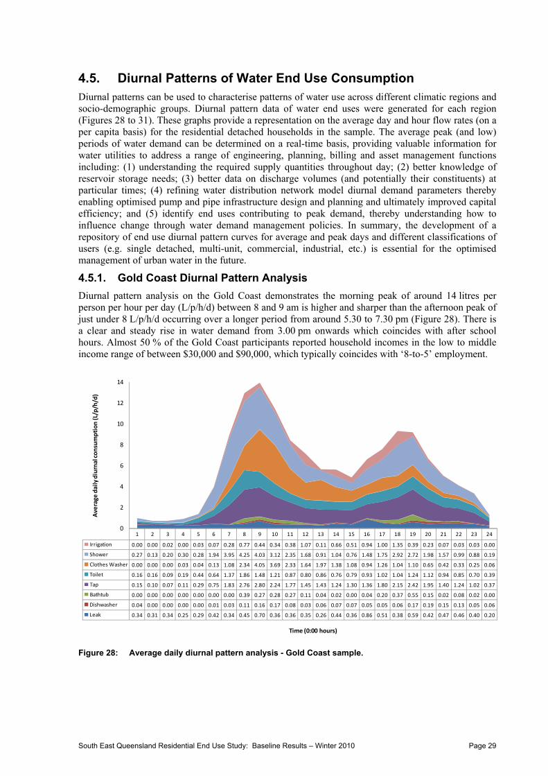
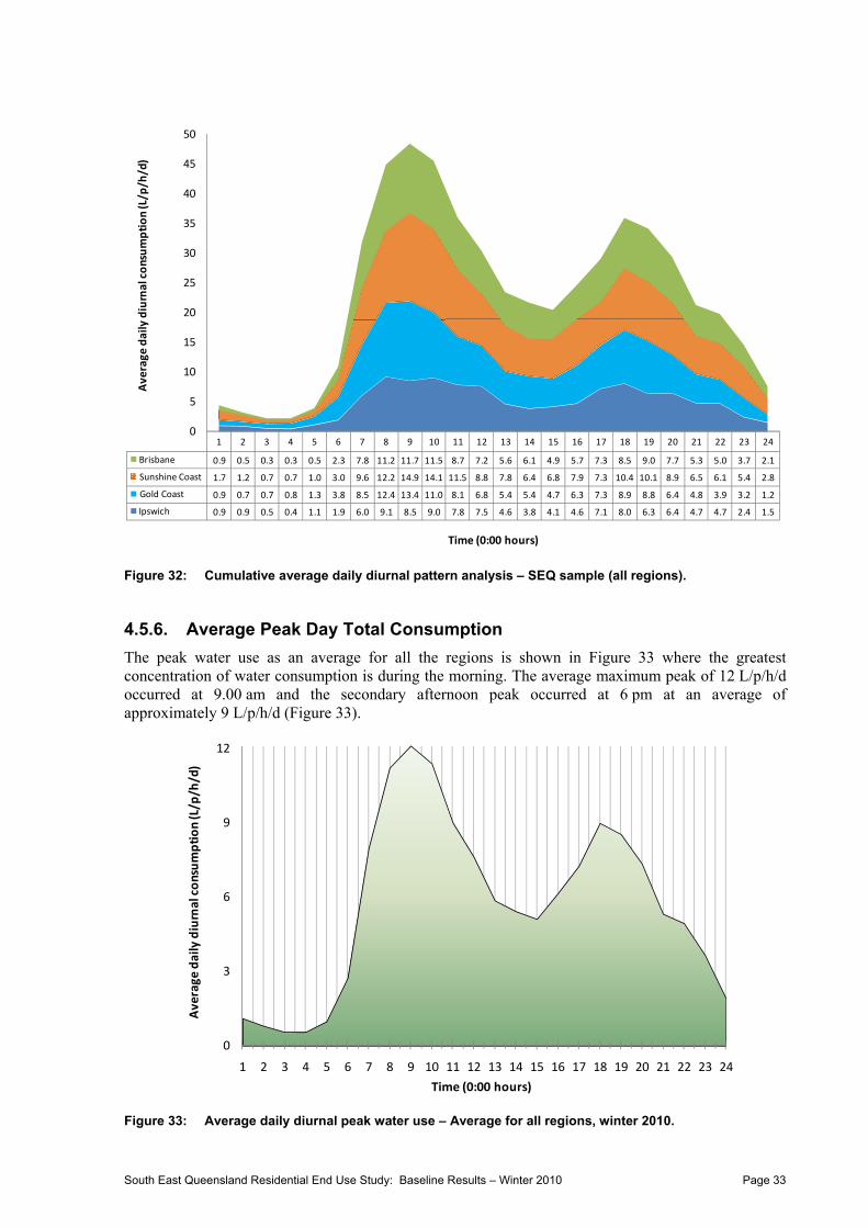
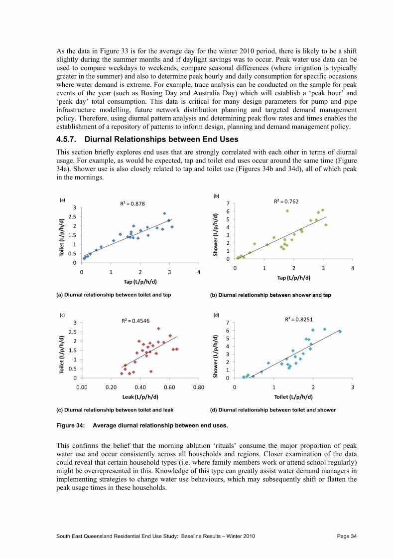
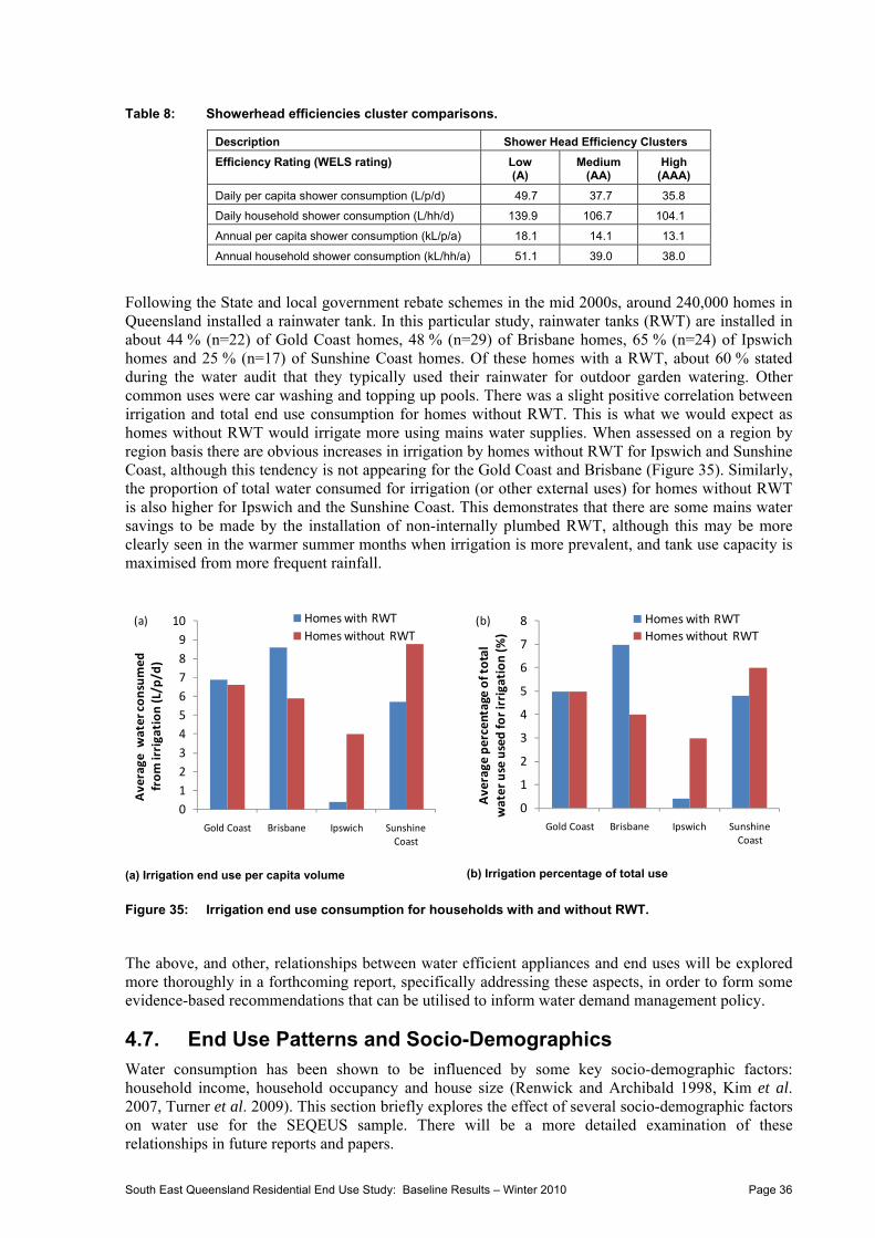
4.5. Diurnal Patterns of Water End Use Consumption .............................................................29 4.5.1. Gold Coast Diurnal Pattern Analysis .............................................................................. 29 4.5.2. Brisbane Diurnal Pattern Analysis .................................................................................. 30 4.5.3. Ipswich Diurnal Pattern Analysis .................................................................................... 31 4.5.4. Sunshine Coast Diurnal Pattern Analysis ....................................................................... 31 4.5.5. SEQ Diurnal Pattern Analysis......................................................................................... 32 4.5.6. Average Peak Day Total Consumption........................................................................... 33 4.5.7. Diurnal Relationships between End Uses....................................................................... 34

4.6. End Use and Water Appliance Efficiencies .......................................................................35

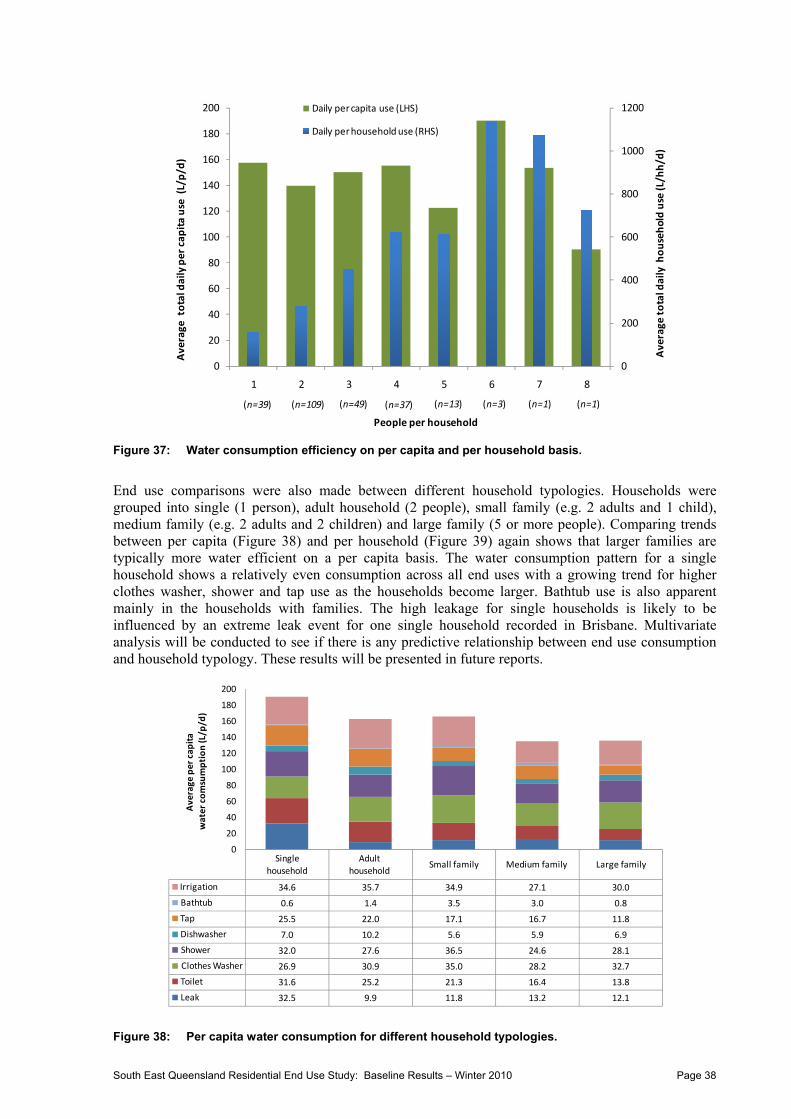
4.7. End Use Patterns and Socio-Demographics .....................................................................36 4.7.1. Income and Household Resident Typology .................................................................... 37 4.7.2. Actual Versus Perceived Water Use Behaviours............................................................ 39

5. Conclusions and Policy Considerations...................................................................44

6. Future Reporting .........................................................................................................45

References ............................................................................................................................46

South East Queensland Residential End Use Study: Baseline Results – Winter 2010 Page iv

LIST OF FIGURES

Figure 1: Average water consumption for common residential end uses sourced from recent Australian studies. ............................................................................................................................. 7

Figure 2: Comparison of indoor water end uses from three Australian water end use studies. ........................ 8 Figure 3: Regions examined in SEQEUS. Inset: location of SEQ..................................................................... 9 Figure 4: June 2010 average daily rainfall data for the study regions............................................................. 10 Figure 5: Comparison of June 2010 average monthly rainfall data for the study regions. .............................. 10 Figure 6: Schematic flow of process for acquisition, capture, transfer and analysis of water flow data. ......... 12 Figure 7: Measurement and data storage equipment. .................................................................................... 12 Figure 8: Frequency and cumulative distribution curves for clothes washer end use. .................................... 14 Figure 9: Frequency and cumulative distribution curves for toilet end use. .................................................... 14 Figure 10: Frequency and cumulative distribution curves for shower end use. ................................................ 15 Figure 11: Frequency and cumulative distribution curves for tap end use........................................................ 15 Figure 12: Frequency and cumulative distribution curves for dishwasher end use........................................... 16 Figure 13: Frequency and cumulative distribution curves for bathtub............................................................... 16 Figure 14: Frequency and cumulative distribution curves for leak end use. ..................................................... 17 Figure 15: Frequency and cumulative distribution curves for irrigation end use. .............................................. 17 Figure 16: Average daily per capita water end use breakdown for all SEQ regions analysed.......................... 19 Figure 17: Comparison of all SEQ per capita water use with SEQEUS total average. ..................................... 20 Figure 18: Household per capita consumption (L/p/d) activity break down for each participant in the

SEQEUS study. ............................................................................................................................... 21 Figure 19: Distribution of water consumption for irrigation end uses. Inset shows correlation between

homes with irrigation end use and total water consumption. ........................................................... 21 Figure 20: Breakdown of average end uses for each region. ........................................................................... 22 Figure 21: Average percentage of total water consumption for each end use across the four regions. ........... 23 Figure 22: Break down of average end uses for the Gold Coast. ..................................................................... 24 Figure 23: Break down of average end uses for Brisbane................................................................................ 25 Figure 24: Break down of average end uses for Ipswich. ................................................................................. 25 Figure 25: Standard deviation for individual end uses across the regions: comparing variance....................... 26 Figure 26: Break down of average end uses for the Sunshine Coast............................................................... 27 Figure 27: Comparison of average end use consumption between SEQEUS data and other end use

studies. ............................................................................................................................................ 28 Figure 28: Average daily diurnal pattern analysis - Gold Coast sample. .......................................................... 29 Figure 29: Average daily diurnal pattern analysis - Brisbane Region. .............................................................. 30 Figure 30: Average daily diurnal pattern analysis - Ipswich Region.................................................................. 31 Figure 31: Average daily diurnal pattern analysis - Sunshine Coast Region. ................................................... 32 Figure 32: Cumulative average daily diurnal pattern analysis – SEQ sample (all regions)............................... 33 Figure 33: Average daily diurnal peak water use – Average for all regions, winter 2010.................................. 33 Figure 34: Average diurnal relationship between end uses. ............................................................................. 34 Figure 35: Irrigation end use consumption for households with and without RWT. .......................................... 36 Figure 36: Relationship between income category, age and average household occupancy........................... 37 Figure 37: Water consumption efficiency on per capita and per household basis. ........................................... 38 Figure 38: Per capita water consumption for different household typologies.................................................... 38 Figure 39: Per household consumption for different household typologies. ..................................................... 39 Figure 40: Comparisons of actual per capita water use with self-identified low, medium and high water

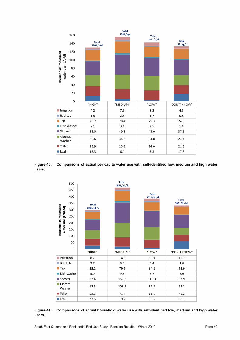
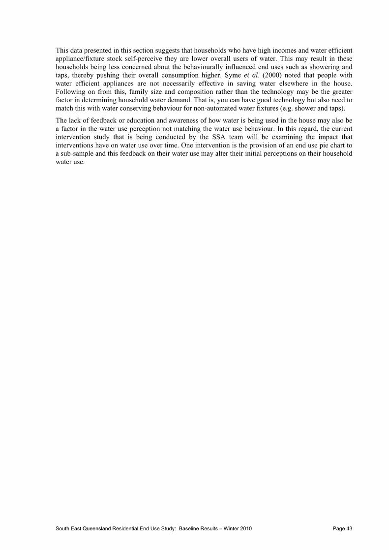
users................................................................................................................................................ 40 Figure 41: Comparisons of actual household water use with self-identified low, medium and high water

users................................................................................................................................................ 40 Figure 42: Selected family characteristics and self-identified low, medium and high water users. ................... 41 Figure 43: Comparisons of income categories with self-identified low, medium and high water users............. 41 Figure 44: Comparisons of washing machine efficiencies with self-identified low, medium and high

water users...................................................................................................................................... 42 Figure 45: Comparisons of washing machine and shower fixture water efficiencies with self-identified

low, medium and high water users. ................................................................................................. 42

South East Queensland Residential End Use Study: Baseline Results – Winter 2010 Page v

LIST OF TABLES

Table 1: Summary of Recent Water End Use Studies..................................................................................... 6 Table 2: General characteristics of monitored households in SEQEUS. ......................................................... 9 Table 3: Climate data for four regions during the period of analysis1............................................................ 10 Table 4: Criteria for sample selection of SEQEUS households. .................................................................... 11 Table 5: Descriptive statistics for SEQREUS winter 2010 data. .................................................................... 13 Table 6: Comparison of average total per capita water use (L/p/d) for dwellings in SEQ.............................. 23 Table 7: Clothes washer efficiency comparisons........................................................................................... 35 Table 8: Showerhead efficiencies cluster comparisons................................................................................. 36 Table 9: Topics to be examined in future SEQREUS technical reports......................................................... 45

South East Queensland Residential End Use Study: Baseline Results – Winter 2010 Page 1

EXECUTIVE SUMMARY

The primary aim of this study was to quantify and characterise mains water end uses in a sample of 252 residential dwellings located within South East Queensland (SEQ). This report presents the methodology, results and discussion on the baseline end use analysis for a two-week period in winter (June 2010) and forms part of the Informed Decision Making research theme for the Urban Water Security Research Alliance.

A mixed method approach was used, combining high resolution water meters, remote data transfer loggers, household water appliance audits and a self-reported household water use diary. Existing standard water meters were replaced with high resolution meters that are capable of providing 0.014 L/pulse outputs in five second intervals to wireless data loggers. A representative sample of received data was extracted from the database and disaggregated into all end use events associated with the sampled residential households. A water fixture/appliance stock survey on the study sample was conducted in order to qualify how householders interact with such stock. In addition to the stock survey, each household was asked to complete a water diary where as many internal and external water use events as possible were recorded over a seven-day period. Both the water diary and stock survey greatly assisted data analysts to conduct the water end use trace analysis process. The water diary in particular allowed for greater accuracy in matching water flow patterns with a specific water appliance.

A total of 252 homes was analysed for mains water end uses. This comprised 87 in the Gold Coast, 61 in Brisbane, 67 in Sunshine Coast and 37 in Ipswich. The total represents approximately 80 % of our target sample of 320 homes (80 per region). A number of factors influenced the smaller than expected sample, including logger failures, predominantly due to moisture ingress, poor meter to logger data transfer and some last minute cancellations of participants. It is planned that many of the faulty loggers will have been replaced and are operable in time for the next milestone. We anticipate 300 homes in our sample for the summer 2010/11 end use analysis, which represents nearly 95 % of the initial target.

The SEQ sample average total water consumption of 370.7 litres per household per day (L/hh/d) was recorded during the period of analysis (i.e. winter 2010). This represented a per capita average of 145.3 litres per person per day (L/p/d), compared with the Queensland Water Commission (QWC) reported figure of 154 L/p/d. The relatively small difference between the South East Queensland End Use Study (SEQEUS) and QWC averages are due to a range of sampling factors including: (1) slight disparity in sample characteristics; (2) assumptions embedded into the QWC calculations for per capita water consumption; and (3) biases encountered when recruiting consenting households to a research study (e.g. very high water consumers unlikely to consent). Both the SEQEUS and QWC-based water use averages fell well below the Permanent Water Conservation target of 200 L/p/d as recommended by the State government.

End use breakdown on a per capita basis indicated that, on average, shower 42.7 L/p/d (29 %), tap 27.5 L/p/d (19 %) and clothes washer 31 L/p/d (21 %) comprised the bulk of the water consumption. Almost 70 % (approximately 100 L/p/d) of total consumption was attributed to these three activities. Of note, irrigation made up less than 5 % of average total consumption. Properties located in the Sunshine Coast consumed the most water per capita (171 L/p/d) and per home (472 L/hh/d). Householders in Ipswich were clearly the most conservative water consumers, using an average of 111 L/p/d (305 L/hh/d). Brisbane and Gold Coast had similar average per capita and household total water usage at 144 and 141 L/p/d and 331 and 348 L/hh/d, respectively. The end uses which varied markedly between regions were showers, leaks, and irrigation.

The low measured irrigation volumes may be attributed to the winter season where outdoor watering is typically lower than it is in the hotter, summer climate. Rainfall prior to the measurement period may also have reduced the need for watering. Additionally, there may be tendency for lower external watering to occur due to the sustained change in behaviours as a result of the stringent water restrictions imposed during the recent drought in SEQ. However, of the homes that did irrigate (or used water for external purposes), 20 % contributed to over 80 % of total irrigation water use at an average of 30 L/p/d.


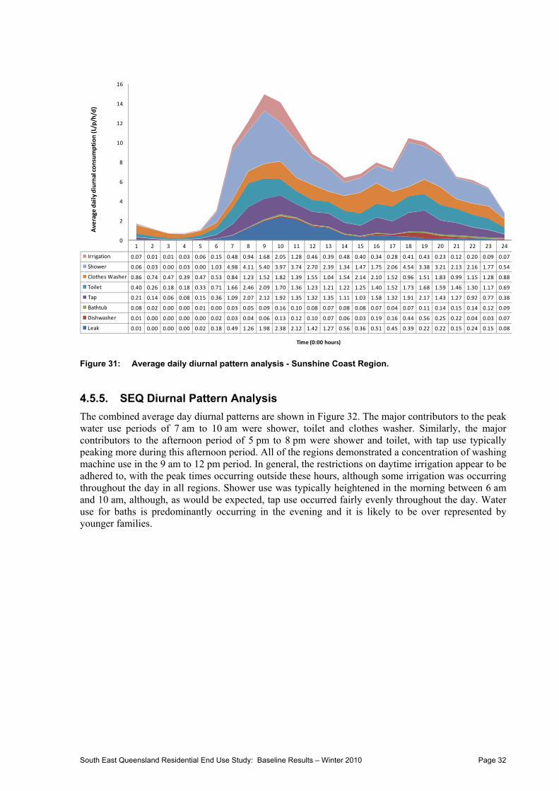
Diurnal patterns demonstrated a concentration of washing machine use in the 9 am to 12 pm period. In general, the restrictions on day time irrigation appear to be adhered to, with the peak times occurring outside these hours, although some irrigation was occurring throughout the day in all regions. Shower use was typically heightened in the mornings and tap usage occurred fairly evenly throughout the day. Water use for baths is predominantly occurring in the evening and it is likely to be over represented by younger families. The average day peak hour flow rate of 12 L/p/h/d occurred at 9.00 am and the secondary afternoon peak hour occurred at 6 pm at an average of 9 L/p/h/d. This is likely to shift slightly during the summer months.

Front loading machines used significantly less water (11.3 L/p/d, p<0.05) than top loaders and a significantly lower proportion (7 %, p<0.05) of total household water was required by front loading machines. There was a trend toward lower water consumption on a per capita and per household basis when high efficiency shower heads were installed. Results show that replacing low with high-efficiency showerheads could save shower end use consumption by nearly 20 %. This study reinforces the benefits of the Home Water Wise Service conducted by the State Government during the drought period.

Some of the households participating in this study had rainwater tanks (RWT) used for external consumption (i.e. not plumbed internally). RWT consumption was not physically monitored; however, their performance can be ascertained through statistical comparisons between households with and without RWT. There was a slight positive correlation between irrigation and total end use water consumption for homes without RWT. The proportion of total water consumed for irrigation is on average higher where no RWT is installed, for all regions with the exception of Brisbane. This demonstrates there are some mains water savings to be made by the installation of RWT. Readers should note that internally plumbed RWTs are outside the scope of this study.

Younger aged households were observed to use less water per capita and this may have some interesting implications for newer developments that are tending toward larger, younger families e.g. master planned communities. There was a disparity between perceived and actual water use behaviour with self identified “high” water users consuming the least and households identifying themselves as “medium” or “low” water users consuming the most water. Washing machine and shower end uses were the most sensitive to misperceptions of water use.

Water demand management key points for stakeholders in this project include:

Still some degree of non-compliant irrigation during 10 am and 4 pm, particularly for homes in the Sunshine and Gold Coasts;

Leaking toilets are more widespread than previously reported; Water efficient fittings for showers and taps are excellent least cost water demand management

options for conserving water, confirming previous studies; Changing to efficient washing machines significantly reduces household consumption; and High per capita water consumption occurs for older, lower income, smaller-sized households. The low water consumption reported for this study confirms the anecdotal and government reporting of a shift in general water consumption post drought in SEQ. The attitudes and water use behaviours of people have generally moved toward a more conservative approach to water use. This increased awareness, together with ongoing water conservation measures for much of SEQ, was likely to maintain a generally low consumption rate of water during winter of 2010. A Summer 2010/11 end use sample will enable better understanding of seasonal influences on water end uses, particularly irrigation.


1. INTRODUCTION

1.1. Introduction and Scope Water security is becoming one of Australia’s greatest issues of concern. Many regions of Australia are facing a severe drought after years of continued lower than average rainfall. South East Queensland (SEQ) has just come through one of its most severe and protracted droughts on record. For this reason, as well as the addition of high population growth and strong economic development, water and its use must be managed very carefully. In an attempt to improve water security, many government authorities have imposed a number of water restrictions and water saving measures to ensure the frugal use of water across the residential, commercial and industrial sectors. Moreover, due to greater social awareness, people are beginning to value water as a precious resource. Behaviour and attitudes toward both potable and recycled water have forever changed, thus requiring renewed understanding of the link between these factors and water end use.

The project provides residential water consumption end use breakdowns at particular points in time. These data can feed into water demand models to forecast supply requirements. Moreover, the analysis of end use data along with stock survey and questionnaire data, reveals the predictors of water demand for different end uses (households demographics, washing machine efficiency, etc.), thus enabling the government and water businesses to target those end uses which can be reduced when required, through targeted communication strategies, rebate programs, etc.

This report is part of a series summarising the output from the South East Queensland End Use Study (SEQEUS) which is one of several key themes investigated through the Alliance. This report presents and discusses the baseline end use analysis for winter 2010 (June 14th to June 28th). The study regions in SEQ are located within the Brisbane, Gold Coast and Ipswich City Councils and Sunshine Coast Regional Council.

1.2. Research Objectives The primary aim of the study is to quantify and characterise mains water end uses in a sample of 250 single detached dwellings across SEQ. Specific objectives for the baseline study are:

to calculate both the household and per capita water consumption volumes of each participating household for the majority of water end use categories (e.g. shower, washing machine, tap, etc.) from households in the study regions;

to undertake a comparative analysis of water end uses between different household demographic categories within the study regions;

to undertake a comparative analysis of water end uses of sampled households with previous end use studies;

to develop average day diurnal pattern curves and explore peak hour flow rates and the end uses underpinning them; and

to conduct some preliminary assessments of the influence of household appliance/fixture efficiency on water end use consumption.


2. BACKGROUND OF WATER END USE RESEARCH

2.1. Introduction Over 750,000 new dwellings are forecast for SEQ to house the expected increase in population from 2.8 to 4.4 million people in 2032 (DIP 2009). The combination of enforced water restrictions and State and local government rebate programs for water efficient fixtures and rainwater tanks has resulted in a large reduction in household water use in SEQ.

Despite the successful outcome for SEQ administering authorities, the demand management approach to reduce water consumption necessitated a ‘reactionary’ approach rather than a proactive one and highlighted the need for more detailed information on how the water is proportioned in households and how this may change both spatially and temporally across SEQ. Thus, the disaggregation of residential water end use should be considered as a critical first step in the development of relevant and successful water policy. More specifically, end use data can facilitate the identification of correlations between water behaviours and key demographical subsets within a population (e.g. income, age, gender and family composition). This information can inform government and water business demand management policy, water rebate program effectiveness and householders’ response to changed water policy. Measured end use data across seasons and regions is the foundation for water consumption predictions and the development of demand forecasting/water distribution network models (Blokker et al. 2010).

2.2. Methods of End Use Measurement

2.2.1. Introduction

Water consumption does not always follow a normal distribution, as the high water users can strongly skew results. Similarly, water consumption patterns and behaviours are highly varied amongst households based on socio-demographics, house size, climate, family composition, water appliances, cultural practices and climate, to name just a few factors. As the end use of water is influenced by a number of subjective factors within a household, surveys or questionnaires are a key component of any end use study, regardless of technology used. Where resources are limited, often household surveys on water use behaviours are the only basis for reporting end uses (e.g. Sivakumaran and Aramaki 2010). The following sections describe the two tiers of end use measurements based on the sophistication of the metering and data capture technology.

2.2.2. Typical End Use Approaches

Most end use studies have a mixed method approach that uses some level of technology with the data capture together with household surveys and/or existing statistical information sourced from various documents (e.g. ABS Census data, council billing data, previous reports). In some instances, residential water demand and end use volumes are predicted using a variety of data. For example, Blokker et al. (2010) simulated residential demand with a stochastic end use model. In this study, the water end use types were compiled from data; frequency of water fixture/appliance use was retrieved from previous household water surveys and intensity of use was determined from water use surveys and technical information from the stock appliance manufacturers. However, this approach can lead to inaccuracies, particularly for subjective end uses such as showers and taps. Additionally, reported appliance flow rates from manufacturers are not always the same as actual measured flow rates as was found by Mead and Aravinthan (2009). Therefore, disaggregating end uses from actual long term measurement and analysis is considered the most robust and accurate approach.

2.2.3. Advanced End Use Measurement

Advanced end use measurement encompasses a range of attributes associated with all components of an end use study, and is not just limited to improved data capture. Advances in methods for data capture, transfer, storage and analysis have improved the resolution of water volume data and made transfer and collection of data substantially more time efficient. Giurco et al. (2008) considers ‘smart metering’ to have the following key elements: real time monitoring, high resolution interval metering (≥10 seconds), automated water meter reading (e.g. drive by, GPRS) and access to data from the internet.


Willis et al. (2009a) used a mix method approach of high resolution water meters (0.014 L/pulse), 10 second interval data logging and detailed household stock inventories to measure and characterise the end uses of 151 dwellings on the Gold Coast. With this level of detail, sophisticated statistical analysis and water demand modelling can be performed with a much higher degree of certainty and fewer (often critical) assumptions embedded within the results. Indeed, Arbués et al. (2003) argue that water pricing modelling, particularly when incorporating time-of-use-tariffs, will only really be useful if a high level of detailed data input data is used.

Data transfer has also improved in recent times, enabling stored data from the loggers to be transferred remotely from the site. Such examples include drive-by technology where data is uploaded while driving past the metered property (e.g. Britton et al. 2009) or data is sent wirelessly via a GPRS system (i.e. email) from the loggers to an external office computer (e.g. Mead and Aravinthan 2009).

As mentioned above, information on the social and behavioural aspects of metered properties, along with an audit of water appliance and fixtures, is absolutely essential for trace flow analysis (Athuraliya et al. 2008; White et al. 2004). Software such as Trace Wizard® has provided a key link between measured data and end use disaggregation (DeOreo and Mayer 1999). However, without a stock inventory and information on water use behaviour/patterns for each dwelling it would be extremely difficult to create meaningful and accurate end use templates. Ultimately, a diary should be kept for a week or more, recording the time and nature of as many water events as possible at the metered dwelling. Retrospective analysis could then identify the water event with the trace flow and match the end use type. Having the benefit of a water diary is not always possible and it requires a high level of commitment from the participants. Nevertheless, this was part of the advanced end use measurement approach for the SEQEUS study and has, to date, had an excellent return rate from the participants. Others such as O’Toole et al. (2009) and Wutich (2009) have also observed self-reported water usage via diaries can be more accurate than verbal estimations during interviews, especially for some end uses such as toilets (O’Toole et al. 2009).

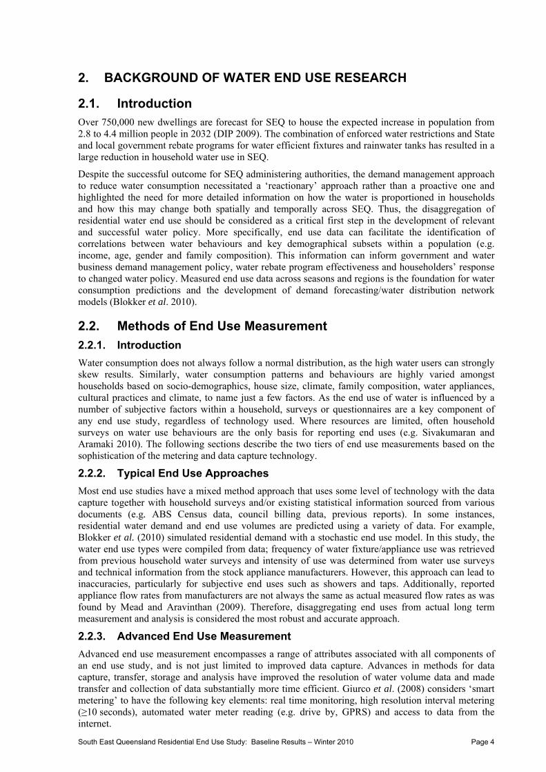
2.3. Typical Residential End Uses A summary of recent end use studies outlining methods and selected results is presented in Table 1. In Australia, there have been only a few end uses studies using a combination of metering technology, household surveys and end use software (i.e. Trace Wizard®) (Table 1). There are two frequently cited studies which have been conducted earlier; one in Perth (Loh and Coghlan 2003) and the other in Melbourne (Roberts 2005). Willis et al. (2009a) have reported more recently on water end uses from 151 dwellings in a development serviced by dual reticulated supplies (recycled water and mains water). Mead and Aravinthan (2009) reported on a small study of 10 residential properties in Toowoomba, west of Brisbane, Queensland. Internationally, several studies have been conducted in the United States of America (Mayer and DeOreo 1999; Mayer et al. 2004) as well as a recent study in New Zealand (Heinrich 2007).


Table 1: Summary of Recent Water End Use Studies.

Study Location Sample size (hh)

Sample regime Dwelling type/s

Data capture Data transfer and analysis

Selected results (in L/p/d unless otherwise stated)

Reference

2010 – Estimation of end uses in Sri Lankan township

Trincomalee

Sri Lanka

106 One off household surveys and interviews

Township dwellings

Monthly tap supply data and household questionnaires from surveys collected. Results used to compare water end use patterns amongst similar household groups.

Total 139 L/p/d:

bathing 37, laundry 21, toilet 19,

washing and cooking 26

Sivakumaran and Aramaki (2010)

2009 - Gold Coast Watersaver EUS

Gold Coast 151 Winter 2008 and Summer 2009

Single, detached, dual reticulation

Actaris CT5-S meters, Aegis Datacell R series loggers, 10 sec. int.

Manual download to PC in-situ Trace Wizard®

Total 157 L/p/d (winter):

shower 50, clothes washer, 30toilet 21, leaks 2.

Indoor 139.

Willis et al. (2009a,b)

2008 – USQ Investigation of domestic water end use

Toowoomba 10 Continuous for 138 days

Single detached

Actaris CT5-S meters, Monita R series loggers, 10 sec. int.

Wireless download – weekly email Trace Wizard®

Total 112 L/p/d:

shower 49 clothes wash 25

taps 17, toilets 14. Low outdoor water use reflected Level 5 restrictions.

Mead (2008)

2007 – NZ Water End Use and efficiency project

Auckland region

51 6 months: across summer and winter

Single, detached

Neptune disc meter, 34.2 pulses/L, Branz data loggers, 10 sec int.

Manual download to PC. Trace Wizard®

Total 112 L/p/d:

shower 50, clothes wash 43

taps 21, toilets 33

Heinrich (2006)

2005 – Yarra Valley Water Residential End Use Measurement study

Yarra Valley, VIC, Aust.

100 2 x 2 wks summer and winter

Single detached

Actaris CT5 modified to 72 pulses/L. Monatec XT logger, 5 sec int.

Manual download into MS Access database. Trace Wizard®

Indoor 169 L/p/d:

shower 49, clothes washer 40, toilet 30.

Outdoor 32% of total

Roberts (2005)

2004 - Tampa Water Department Residential Water Conservation Study

Florida, USA 26 2 wk baseline data + 2 x 2 wk data post retrofit

High end users (230 L/p/d)

Trident T-10 or Badger 25 meters, Meter-Master loggers,

Downloaded to PC and Trace Wizard®

Indoor 291 and 147 L/p/d (baseline and post retrofit respectively):

48 and 34 shower, 55 and 30 clothes wash, 67 and 30 toilet, 71 and14 leaks.

Mayer et al. (2004)

1998 – 2001 WA Water Corporation Perth Domestic Water Use study

Perth, WA, Aust.

120 and 600

surveys

18 months for single and 13 months for multi

Single and multi

Smart meters and loggers (unspecified)

Manual download to PC in-situ and Trace Wizard®

420 kL/hh/y (single dwelling results only shown): clothes wash 27, bath/shower 33, toilets 21. 155 indoor (42% of total).

Loh and Coghlan (2003)

1998 USA and Canada residential end use – AWWA

USA/Canada 1,188 2 x 2 wks summer and winter

Single detached

Magnetic water meters, Meter Master 100EL logger, 10 sec int.

Manual logger and download ex-situ and Trace Wizard®

Indoor 262 L/p/d:

clothes washer 57, shower 44, toilet 70

Mayer et al. (1998)


End uses of water in residential households include showers, clothes washers, toilets, indoor taps, leakages, and outdoor irrigation (Mayer and DeOreo 1999). Average daily end use consumption per capita for the four most recent Australian studies is presented in Figure 1 (error bars represent standard deviation). Bathroom (toilet, shower) and laundry activities generally place the greatest residential indoor demand on potable water with a combined daily usage averaging around 95 litres per person (L/p). At an average of nearly 40 litres per person per day (L/p/d), cumulative tap usage throughout the day may not be evident to individual users and could be a significant area to target in future demand management initiatives.

Figure 1: Average water consumption for common residential end uses sourced from recent Australian studies.

Notwithstanding the inherent differences in household occupancy rates between studies, the volume of water end use varies, often substantially, between research categories and regions (Figures 1 and 2). Not surprisingly, the water appliances that have fixed water volumes and cycles (dishwasher, clothes washer, toilets) have less variation per person than the water fixtures that are manually operated by individuals (taps). In this instance, the household survey and water diaries would play a strong role in accurately categorising the ‘manual’ water events and assist in teasing out the simultaneous events in a trace flow analysis.

Variation between studies can be driven by outdoor end uses (e.g. irrigation) as shown in Figure 1 where the standard deviation is ±39.6 L/p/d. Irrigation itself is typically a result of region specific factors such as climate, plant species, restriction regime and garden size (Loh and Coghlan 2003; Roberts 2005). End use consumption can also vary within studies, particularly when doing a comparative analysis of seasons i.e. winter versus summer (e.g. Heinrich 2007; Roberts 2005; AWWA 1998). Outdoor irrigation can be relatively easy to detect in a flow pattern where an automatic irrigation system is used or a continuous flow rate through a standard hose nozzle for an extended period (i.e. 30 minutes). However, sporadic irrigation events with trigger nozzle hoses are significantly more difficult to accurately disaggregate using a single meter and Trace Wizard approach.

ToiletShower / bath

Clothes washer

Dish washer

Taps Leaks Indoor Outdoor

Series1 23.5 46.2 32.5 2.3 35.3 8.3 145.3 39.6

0

20

40

60

80

100

120

140

160

180

Average per capita consumption (L/p/day) Sources:

Willis et al (2009)Mead and Aravinthan (2009)Heinrich (2007)Roberts (2005)Loh & Coghlan (2003)


Leaks are an important end use that is often overlooked by consumers if they are not visually evident. Post meter leakage can account for up to 10 % of total water consumption in the residential sector where a small number of homes can account for a large percentage of consumption. For example, Britton et al. (2009) found that 2 % of the meters accounted for 24 % of the night time consumption. The contribution of leaks can also vary across households and regions, as shown in Figure 2, where the range is 2 % to 8 % of the total indoor water usage (Figure 2).

Figure 2: Comparison of indoor water end uses from three Australian water end use studies.

BATH/ SHOWER31%

LEAKS8%

TAP17%

TOILET18%

WASHING MACHINE

26%

BATH/ SHOWER 33%

LEAKS2%

TAP15%

TOILET22%

WASHING MACHINE

28%

MELBOURNE (Roberts 2006)Mean internal‐ 169 L/p/dMean total‐ 226 L/p/d

Mean internal‐ 139 L/p/dMean total‐ 157 L/p/d

GOLD COAST (Willis et al. 2009)

PERTH (Loh and Coghlan 2003)

Mean internal‐ 155 L/p/dMean total‐ 335 L/p/d

BATH/ SHOWER42%

LEAKS1%

TAP20%

TOILET15%

WASHING MACHINE

22%


3. RESEARCH METHODS

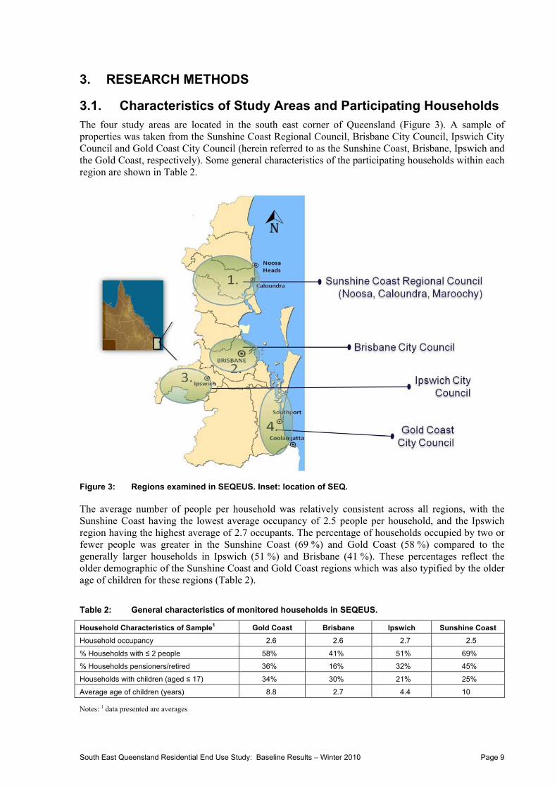
3.1. Characteristics of Study Areas and Participating Households The four study areas are located in the south east corner of Queensland (Figure 3). A sample of properties was taken from the Sunshine Coast Regional Council, Brisbane City Council, Ipswich City Council and Gold Coast City Council (herein referred to as the Sunshine Coast, Brisbane, Ipswich and the Gold Coast, respectively). Some general characteristics of the participating households within each region are shown in Table 2.

Figure 3: Regions examined in SEQEUS. Inset: location of SEQ. The average number of people per household was relatively consistent across all regions, with the Sunshine Coast having the lowest average occupancy of 2.5 people per household, and the Ipswich region having the highest average of 2.7 occupants. The percentage of households occupied by two or fewer people was greater in the Sunshine Coast (69 %) and Gold Coast (58 %) compared to the generally larger households in Ipswich (51 %) and Brisbane (41 %). These percentages reflect the older demographic of the Sunshine Coast and Gold Coast regions which was also typified by the older age of children for these regions (Table 2).

Table 2: General characteristics of monitored households in SEQEUS.

Household Characteristics of Sample1 Gold Coast Brisbane Ipswich Sunshine Coast

Household occupancy 2.6 2.6 2.7 2.5

% Households with ≤ 2 people 58% 41% 51% 69%

% Households pensioners/retired 36% 16% 32% 45%

Households with children (aged ≤ 17) 34% 30% 21% 25%

Average age of children (years) 8.8 2.7 4.4 10

Notes: 1 data presented are averages


0

20

40

60

80

100

120

Gold Coast Brisbane Sunshine Coast Ipswich

Average monthly rainfall (m

m) June, 2010 Average for June (historical data)

The climate data for the study regions during the period of analysis (14th to 28th June, 2010) is presented in Table 3. As each region covered a long and relatively narrow area, climate data was averaged from two weather stations (except for Ipswich). Minimum temperatures varied from 6.4°C in Ipswich to around 13°C on the coast. Maximum temperatures were less variable at around 21°C across all regions (Table 3).

Table 3: Climate data for four regions during the period of analysis1.

Study Region Average Min. (°C)

Average Max. (°C)

Rainfall (mm) No. of wet days2 in month of June

Gold Coast3 13.1 (±2.27) 21.3 (±0.8) 19.5 (±13.4) 4

Brisbane4 9.9 (±2.6) 21.4 (±0.9) 5.1 (±1.0) 2

Ipswich5 6.4 (±3.6) 21.8 (±1.2) 2 (±0.6) 1

Sunshine Coast6 13.0 (±1.6) 21.4 (±0.9) 47.4 (±3.4) 7

Notes: 1 Data taken from Bureau of Meteorology (BOM) http://www.bom.gov.au/climate/data/index.shtml; 2 Number of days where rainfall exceeded 1mm; 3 average of Coolangatta and Gold Coast BOM stations; 4 average of Brisbane Airport and Archerfield BOM stations; 5

Amberley BOM station; 6 average of Maroochydore and Tewantin BOM stations, 7 (±x) indicates standard deviation from mean for the period of analysis.

As is typical for SEQ, winter rainfall was low at an average of 22 mm for the month of June across the four regions, although the standard deviation is high (~18 mm) as a result of some higher rainfall events on the Sunshine Coast (Figure 4). The number of wet days in June (≥ 1 mm rainfall) ranged from one in Ipswich to seven in Tewantin (northern Sunshine Coast). Rainfall was markedly lower than the long term averages reported for all regions (Figure 5).

0

2

4

6

8

10

1 4 7 10 13 16 19 22 25 28

Daily rainfall (mm)

Gold Coast

0246810121416

1 4 7 10 13 16 19 22 25 28

Daily rainfall (mm)

Sunshine Coast

0

2

4

6

8

10

1 4 7 10 13 16 19 22 25 28

Daily rainfall (mm)

Day of month

Brisbane

0

2

4

6

8

10

1 4 7 10 13 16 19 22 25 28

Daily rainfall (mm)

Day of month

Ipswich

Figure 4: June 2010 average daily rainfall data for the study regions.

Figure 5: Comparison of June 2010 average monthly rainfall data for the study regions.


3.2. Sample Selection Process A sub-sample for the SEQEUS project was generated from the larger SSA Demand Management study which involved the completion of a questionnaire of over 1,500 homes across SEQ. From this pool, a smaller sub-sample of homes in each study region consented to the SEQEUS project. A filtering and quality control process was applied to each of the households that consented to be a part of the SEQEUS. Each property was visually inspected prior to being selected for the final sample. Key criteria for sample selection are listed in Table 4. Properties identified as having an internally plumbed rainwater tank or alternative supply source were not included in this study. The study sought to target just mains-only supplied detached dwellings, which make up the majority of residential stock at present. Knowledge on household occupancy and family characteristics was extracted from the SSA household survey response database.

Table 4: Criteria for sample selection of SEQEUS households.

Criteria Comment / Justification for Criteria

Consented to end use study Ethical Clearance requirement for all collaborating research partners.

Residential single, detached dwelling

Required to have a single residential water meter specific only to the property being metered in order to capture single household data.

No internally plumbed rainwater tank. Rainwater tank for external use permitted.

Toilet and/or laundry end uses would be sourced from the rain tank and thus could not be measured by mains water meter. All internal end uses needed to be measured in this study. Rainwater tanks used predominately for external use only (i.e. not plumbed in to household) were accepted and this fact documented in the water audit to allow irrigation comparisons.

Water meters accessible and readily replaced with Smart Meters and associated loggers.

Water meters need to be replaced with minimum disturbance to property. Data transfer requires clear signal. Concrete lid may reduce reception. In summary, the site was reviewed to ensure that it was fit-for-purpose for equipment installations and data collection reliability.

Owner-occupied household Due to consent reasons and that water bills are payed for by the home owner (i.e. landlord), only home owners have been included in the study. Also, rental households are typically transient and can move every 6-12 months, thus not providing a good sample for seasonal comparisons.

3.3. End Use Measurement The relationship between smart metering equipment, household stock inventory surveys and flow trace analysis is shown in Figure 6. Essentially, a mixed method approach was used to obtain and analyse water use data:

Physical measurement of water use via smart meters with subsequent remote transfer of high resolution data; and

Documentation of water use behaviours and compilation of water appliance stock via individual household audits and self-reported water use diaries.

3.3.1. Instrumentation for Data Capture

Standard council residential water meters were replaced with Actaris CTS-5 water meters. These ‘smart’ meters measure flow to a resolution of 72 pulses/L or a pulse every 0.014 L. The smart meters were connected to Aegis Data Cell series R-CZ21002 data loggers. The loggers were programmed to record pulse counts at five second intervals. Each logger was wired to a meter, labelled and activated prior to installation to reduce reliance on external plumbing contractors to prepare and activate the equipment.


Figure 6: Schematic flow of process for acquisition, capture, transfer and analysis of water flow data.

The installations were conducted by approved plumbing contractors. A pilot study for the Gold Coast region (Beal et al. 2010) indicated that the following factors were critical in ensuring a high quality installation process which would substantially reduce the possibility of water ingress and subsequent data loss:

waterproofing all seals including wire connections and aerial fittings on loggers (Figure 7a);

a minimum of three days between silicone work and installation of loggers to allow for sufficient sealing;

replacing standard sized meter boxes with a wider and deeper box to fully accommodate meter and logger and eliminate the need for a forced installation (see Figure 7b); and

developing a thorough quality assurance program including a weekly review of all emails sent by loggers to ensure satisfactory data quality and frequency.

(a) Waterproofed logger. (b) Installed smart meter and data logger.

Figure 7: Measurement and data storage equipment.


3.3.2. Data Transfer and Storage

As the loggers were wireless, data was transferred remotely to a central computer at Griffith University through a GPRS network via email. Removable SIM cards were affixed into each logger and tested prior to installation in the field. The frequency of transfer was weekly which amounted to approximately 120,000 data records. The data was emailed to two separate email addresses, one within Griffith University and an external address to serve as a backup as the data in the loggers were not stored indefinitely. Raw data files, in ASCII format, were then modified into .txt files for subsequent trace flow analysis.

3.3.3. Data Analysis

End use data in .txt file form was analysed by Trace Wizard® software version 4.1 (Aquacraft 2010).

Water diaries and stock appliance audits were used to help identify flow trace patterns for each household. Once a template was created for each household, data for the two-week period 14th to 28th June 2010 was analysed. Trace Wizard® software was used in conjunction with water audits and water diaries to analyse and disaggregate consumption into toilets, taps, leaks, irrigation, shower, clothes washer, bathtub and dishwasher. An MS Excel™ spreadsheet was generated as a final output for a more detailed statistical trend analysis and the production of charts.

3.4. Statistical Interpretation

3.4.1. Distribution and Variability of Water Consumption End Uses

Water consumption can substantially vary within and between sample populations. As a result of this variability, and hence high standard deviation of data points from the mean, the water consumption data does not always follow a statistically normal distribution. In terms of water end use consumption, this holds true for certain end uses such as leaks and irrigation where there is typically high variation within a sample. This variation can be seen in Table 5 where the standard deviation is considerably greater than the average for leaks, dishwasher, bath tub and irrigation. Each of these end uses is characterised by being an optional or low occurrence end use. However, the end uses that exhibit normal distributions are typically found in every home at generally similar volumes and frequencies. For example, toilet, shower, tap usage and clothes washing machines are all constant or typical features of all homes and while their volumes may vary between each household (Table 5) they don’t tend to vary widely within the sample, as shown in Figures 8 to 11. Conversely, there is wide variation and non-normal distributions shown for dishwashers, bathtubs, leaks and irrigation (Figures 12 to 15).

Table 5: Descriptive statistics for SEQREUS winter 2010 data.

Statistic

Leak

L/p/d

Toilet

L/p/d

Clothes Washer

L/p/d

Shower

L/p/d

Dish washer

L/p/d

Tap

L/p/d

Bathtub

L/p/d

Irrigation

L/p/d

Total

L/p/d

Average 9.0 23.9 30.9 42.7 2.5 27.5 1.8 7.0 145.3

Standard Deviation

37.8 15.7 26.8 33.3 4.7 16.6 7.2 15.1 86.7

First Quartile

0.5 14.3 12.8 21.9 0.0 15.5 0.0 0.0 92.8

Median 1.3 20.7 25.2 34.2 1.2 24.1 0.0 0.0 124.3

Third Quartile

4.0 29.2 40.1 53.3 3.7 36.0 0.0 6.1 168.9


0%

10%

20%

30%

40%

50%

60%

70%

80%

90%

100%

0

5

10

15

20

25

30

35

40

0 5101520253035404550556065707580859095

100

More

Cumultaive freq

uency (%)

Freq

uen

cy distribution (no. of h

omes)

Per capita water consumption for clothes washer (L/p/d)

Brisbane

Gold Coast

Sunshine Coast

Ipswich

All

Brisbane

Gold Coast

Sunshine Coast

Ipswich

All

Figure 8: Frequency and cumulative distribution curves for clothes washer end use.

0%

10%

20%

30%

40%

50%

60%

70%

80%

90%

100%

0

5

10

15

20

25

30

35

40

45

50

0 2 4 6 8

10

12

14

16

18

20

30

40

50

60

70

80

Cumultaive freq

uency (%)

Freq

uen


omes)

Per capita water consumption for toilets (L/p/d)

Brisbane

Gold Coast

Sunshine Coast

Ipswich

All

Brisbane

Gold Coast

Sunshine Coast

Ipswich

All

Figure 9: Frequency and cumulative distribution curves for toilet end use.


0%

10%

20%

30%

40%

50%

60%

70%

80%

90%

100%

0

5

10

15

20

25

30

0 5101520253035404550556065707580859095

100

More

Cumultaive freq

uency (%)

Freq

uen


omes)

Per capita water consumption for shower L/p/d)

Brisbane

Gold Coast

Sunshine Coast

Ipswich

All

Brisbane

Gold Coast

Sunshine Coast

Ipswich

All

Figure 10: Frequency and cumulative distribution curves for shower end use.

0%

10%

20%

30%

40%

50%

60%

70%

80%

90%

100%

0

5

10

15

20

25

30

2 6

10

14

18

22

26

30

34

38

42

46

50

54

58

More

Cumultaive freq

uency (%)

Freq

uen


omes)

Per capita water consumption for tap (L/p/d)

Brisbane

Gold Coast

Sunshine Coast

Ipswich

All

Brisbane

Gold Coast

Sunshine Coast

Ipswich

All

Figure 11: Frequency and cumulative distribution curves for tap end use.


0%

10%

20%

30%

40%

50%

60%

70%

80%

90%

100%

0

10

20

30

40

50

60

70

80

90

100

110

0 1 2 3 4 5 6 7 8 9

10

More

Cumultaive freq

uency (%)

Freq

uen


omes)

Per capita water consumption for dishwasher (L/p/d)

Brisbane

Gold Coast

Sunshine Coast

Ipswich

All

Brisbane

Gold Coast

Sunshine Coast

Ipswich

All

Figure 12: Frequency and cumulative distribution curves for dishwasher end use.

0%

10%

20%

30%

40%

50%

60%

70%

80%

90%

100%

0

20

40

60

80

100

120

140

160

180

200

0 1 2 3 4 5 6 7 8 9

10

More

Cumultaive frequency (%)

Frequency distribution (no. of homes)

Per capita water consumption for bathtub (L/p/d)

Brisbane

Gold Coast

Sunshine Coast

Ipswich

All

Brisbane

Gold Coast

Sunshine Coast

Ipswich

All

Figure 13: Frequency and cumulative distribution curves for bathtub.


0%

10%

20%

30%

40%

50%

60%

70%

80%

90%

100%

0

10

20

30

40

50

60

70

80

90

100

110

1 2 3 4 5 6 7 8 9

10

11

12

13

14

15

16

17

18

19

20

More

Cumultaive freq

uency (%)

Freq

uen


omes)

Per capita water consumption for leaks (L/p/d)

Brisbane

Gold Coast

Sunshine Coast

Ipswich

All

Brisbane

Gold Coast

Sunshine Coast

Ipswich

All

Figure 14: Frequency and cumulative distribution curves for leak end use.

0%

10%

20%

30%

40%

50%

60%

70%

80%

90%

100%

0

10

20

30

40

50

60

70

80

90

100

110

0 1 2 3 4 5 6 7 8 9

101112

13141516

17181920

25303540

More

Cumultaive frequency (%)

Frequency distribution (no. of homes)

Per capita water consumption for irrigation (L/p/d)

Brisbane

Gold Coast

Sunshine Coast

Ipswich

All

Brisbane

Gold Coast

Sunshine Coast

Ipswich

All

Figure 15: Frequency and cumulative distribution curves for irrigation end use.


3.4.2. Calculation of Household and Per Capita Water End Uses

The average per household water use (L/hh/d) has been calculated by taking an average of all the individual per household water use data measured from each home. Similarly, the average per capita water use of litres per person per day (L/p/d) was calculated by taking the arithmetic mean of all the individual per capita data calculated from each home. This calculation was completed for each region and the total sample. For reporting the overall average per capita figure, an average was taken from all the individual per capita data across all regions (e.g. average from n=252 individual data points) using known household occupancy for each home. This method provides an accurate picture of the average per capita and household usage of the analysed sample and is a preferred method when accurate household level data is available, as is the case in the SEQREUS (Arbués et al. 2003). It means that the per capita (L/p/d) data can be used as the basic building block for all further calculations as it can be compared with other reported end use studies and provide estimates for urban water consumption for similar cities of varying household occupancy.

However, readers should note that overall average per capita end use values for a region (or for the total sample) and the equivalent household end use values are not interchangeable using an average region or total sample household occupancy scaling factor. This is due to the creation of a new composite per capita statistical distribution for each water end use when dividing each household’s consumption by its occupancy. This per capita end use distribution varies from the household distribution, especially for those end uses which are not normally distributed (e.g. leaks, irrigation, dishwasher, bathtub)as shown in Figures 8 to 15.

The other method for calculating regional or total sample per capita water end use uses can be to take the sum of individual household usage and divide by the sum of the number of occupants. Note that this method will give a slightly different number to the method described above, i.e. the individual L/p/d dataset has a different distribution to the sum of all data divided by sum of all occupants. Nonetheless, readers may opt to calculate per capita end uses this way, by dividing the reported household end use break down by the average sample size for that particular region or the total sample.


4. RESULTS AND DISCUSSION

4.1. Sample Size For this winter 2010 baseline report, 252 homes were analysed for mains water end uses. This comprised 87 in the Gold Coast, 61 in Brisbane, 67 in Sunshine Coast and 37 in Ipswich. The total represents approximately 80 % of our target sample of 320 homes (80 per region). A number of factors influenced the lower than expected sample including: logger failures predominantly due to moisture ingress; poor meter to logger data transfer; unsuitable existing meters (i.e. in a few cases atypical diameter of existing meters could not fit the larger diameter smart meters); aged service pipe (i.e. changing meters may affect the integrity of the corroded pipeline and meter outlets); and some last minute cancellations of participants. In Ipswich in particular, there were many water meters that were not suitable due to location, different sized connections or age of service pipe. Finally, there were two homes that had not had their water audits completed as they were overseas for a long period. Most of these factors were unpredictable and unavoidable. It is planned that many of the faulty loggers will have been replaced and are operable in time for the next milestone. We anticipate 300 homes in our sample for the summer 2010/11 end use analysis, which represents nearly 95 % of the initial target.

Notwithstanding the above, the sample size of 252 is sufficient for a residential end use study. The SEQEUS sample is a good representation of SEQ households with a strong mix of family types, income categories and household occupancies. Additionally, results suggest that the data obtained from this study compares well with other estimations of household consumption (i.e. weekly reports from QWC). This is discussed in more detail in subsequent sections of this report.

4.2. Overall Water Consumption Trends An average total water consumption of 370.7 litres per household per day (L/hh/d) was recorded during the period of analysis. This represented a per capita average of 145.3 L/p/d (Figure 16).

Figure 16: Average daily per capita water end use breakdown for all SEQ regions analysed.

Leak 9 L/p/d(6%)

Toilet 23.7 L(16.5%)

Clothes Washer 31 L/p/d(21%)Shower 42.7

L/p/d(29.5%)

Dishwasher2.5 L/p/d

(2%)

Tap 27.5 L/p/d(19%)

Bathtub1.8 L/p/d (1%)

Irrigation7 L/p/d (5%)

Total average = 145.3 L/p/d


0

50

100

150

200

250

300

350

Jan‐05

Apr‐05

Jul‐05

Oct‐05

Jan‐06

Apr‐06

Jul‐06

Oct‐06

Jan‐07

Apr‐07

Jul‐07

Oct‐07

Jan‐08

Apr‐08

Jul‐08

Oct‐08

Jan‐09

Apr‐09

Jul‐09

Oct‐09

Jan‐10

Apr‐10

Jul‐10

Average

monthly per capita water use (L/p/d)

Time (months)

QWC water use

SEQREUS145 L/p/d

No restrictions

Level1

Level2

Level3

Level4

Level5

Level6

HighLevel

MediumLevel

PWCM

Target 140 L/p/d

Target 170L/p/d

Target 200 L/p/d

In comparison, for the same period, the QWC reported a per capita water use of 154 L/p/d (QWC 2010). The relatively small difference between the SEQEUS and QWC averages is due to a range of sampling factors including: (1) slight disparity in sample characteristics; (2) biases encountered when recruiting consenting households to a research study (e.g. very high water consumers unlikely to consent); and (3) assumptions embedded in the QWC calculations for per capita water consumption. In terms of the last point, the residential per capita water usage for SEQ is calculated based on bulk water use over a weekly period and as such there is an inherent assumption that a certain percentage of businesses are included within this bulk water measurement. Additionally, there will be some bias in the SEQEUS sample due to the smaller size of the sample compared with QWC database and the possibility of a slight overrepresentation of low water consumers due to their involvement in this study.

Both the SEQEUS and QWC-based water use averages fell well below the Permanent Water Conservation Measures (PWCM) target of 200 L/p/d as recommended by the State government (Figure 17). Furthermore, the average water consumption for the regions monitored were roughly equivalent to the water use achieved during enforced high and medium-level water restrictions. This is an encouraging indication that there is some long-term behavioural shift in residential consumers as water use remains generally low regardless of the drought ‘breaking’, water supply dams in SEQ recording over 90 % capacity, and a relaxation on external water usage.

Figure 17: Comparison of all SEQ per capita water use with SEQEUS total average. End use break down on a per capita basis indicated that, on average, shower 42.7 L/p/d (29 %), tap 27.5 L/p/d (19 %) and clothes washer 31 L/p/d (21 %) comprised the bulk of the water consumption (Figure 16). Almost 70 % (approximately 100 L/p/d) of total consumption was attributed to these three activities. Interestingly, water consumption for irrigation and general outdoor purposes was found to be low, at an average of only 7 L/p/d, which is less than 5 % of total consumption (Figure 16).

The household per capita water consumption activity break down is shown in Figure 18. Water end use breakdowns varied substantially across (and within) the regions examined. This variation is a reflection of several factors, including family size and composition, socio-demographic factors and climate. In all homes measured, there was water use from toilet, clothes washer, taps and showers. The remaining end uses analysed: leaks, dishwasher, irrigation and bath tub, were reported in some but not all of the homes.


Figure 18: Household per capita consumption (L/p/d) activity break down for each participant in the SEQEUS study. Typically, the homes that used the most water had a disproportionately high contribution from irrigation. This is shown by the strong correlation observed between total household water use and irrigation (Figure 19). The frequency distribution for irrigation (Figure 19) indicates that half the homes monitored did not register any irrigation use during the period of analysis. The lack of irrigation could be attributed to the winter season where outdoor watering is usually lower than in the hotter summer climate. Additionally, as discussed previously, there may be a tendency for lower external watering to occur due to the change in behaviours as a result of the water restrictions adhered to during the relatively recent drought period. However, of the homes that did irrigate (or use water for external purposes), 20 % contributed to over 80 % of total irrigation water use at an average of 30 L/p/d. This pareto effect has been observed in other residential water use studies (Willis et al. 2009b; Turner et al. 2009) and is a good example of why water restriction policy targets outdoor use to reduce residential demand (Barrett et al. 2009; Inman and Jeffrey 2006; Kenney et al. 2008).

Figure 19: Distribution of water consumption for irrigation end uses. Inset shows correlation between homes with irrigation end use and total water consumption.

0

100

200

300

400

500

600

700

Household W

ater Consumption (L/p/d)

Household ID

Irrigation Bathtub Tap Dishwasher

Shower Clothes Washer Toilet Leak

0

20

40

60

80

100

120

0 6

12 18 24 30 36 42 48 54 60 66 72 78 84 90 96

105

Freq

uen

cy

Water consumption from irrigation (L/p/d)

R² = 0.8927

0

50

100

150

0 500 1000Irrigation water

consum

ption (L/p/d)

Total water consumption (L/p/d)


Dishwashers and leaks were also generally over represented by a small number of households, although the actual consumption was low compared with other end uses at 2.5 and 9 L/p/d, respectively. For the homes that used dishwashers (57 %), the average use was 4.3 L/p/d. Tap use was virtually identical between homes that did and did not use dishwashers. This may provide some evidence to suggest that manually washing dishes is not necessarily more water inefficient compared to dishwashers, especially if rinsing dishes prior to automatic dishwashing is practised. However, there are likely to be several factors influencing these trends which need to be teased out more in future reports.

Daily per capita toilet use was generally distributed quite evenly across the homes in comparison to other end uses such as shower/bath, clothes washer and irrigation (Figure 18). This is commonly reported from other end use researchers (e.g. Willis et al. 2009b, Roberts 2005). Dual flush toilets have been incorporated into homes for some time and are not a new concept relative to water efficient washing machines and low flow taps and shower heads. While Arthuraliya et al. (2008) noted an absence of any significant increases in the use of dual flush toilets, they did observe a clear decrease in flush frequency over the same four-year period (in the early 2000s). This suggests that while adopting new technology in water efficient toilets (e.g. ultra low flow, waterless urinals) maybe slow, the behaviour of toilet use is tending toward a more conservative approach.

4.3. Regional Water Consumption

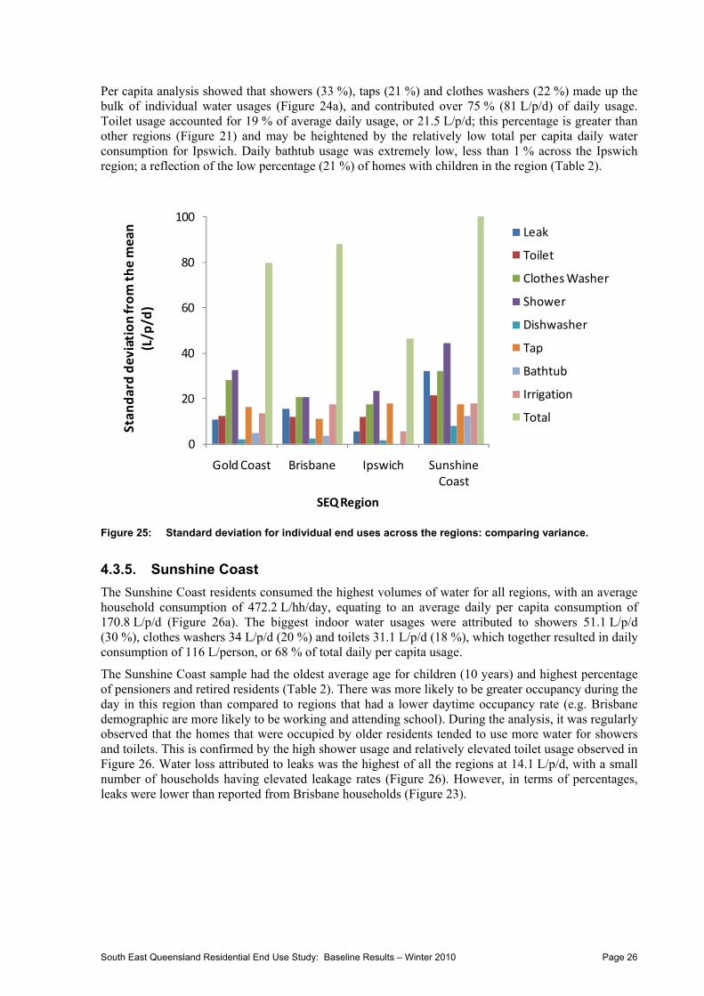
4.3.1. Summary

In terms of water consumption between regions, there were some clear variations between total water use and some end uses on both a per capita and household basis (Figure 20). Properties located in the Sunshine Coast consumed the most water per capita (171 L/p/d) and per home (472 L/hh/d).

Householders included in the Ipswich sample were clearly the most conservative residential water consumers, using an average of 111 L/p/d (305 L/hh/d). Brisbane and Gold Coast had similar average per capita and household total water usage at 144 and 141 L/p/d and 331 and 348 L/hh/d, respectively. The end uses which varied markedly between regions were showers, leaks and irrigation, as shown in Figures 20 and 21.

(a) Per capita end use break down (L/p/d) (b) Per household end use break down (L/hh/d)

Figure 20: Breakdown of average end uses for each region.

Brisbane Gold CoastSunshine Coast

Ipswich

Irrigation 7.2 9.4 6.8 1.7

Bathtub 1.8 1.9 2.9 0.0

Tap 22.7 34.2 26.6 23.0

Dish washer 2.3 1.6 4.2 1.4

Shower 38.6 40.9 51.1 36.3

Clothes Washer 35.8 27.9 34.0 24.5

Toilet 22.0 20.6 31.1 21.4

Leak 13.3 4.3 14.1 2.9

0

25

50

75

100

125

150

175

PER

CAPITA

Average water consumption

(L/p/d)

144

171

111

141

(a)

Brisbane Gold CoastSunshine

CoastIpswich

Irrigation 14.4 19.6 11.0 6.8

Bathtub 5.7 2.0 8.6 0.2

Tap 52.9 82.5 66.0 56.4

Dish washer 7 4.3 9.3 5.2

Shower 94.8 104.2 155.8 107.0

Clothes Washer 89.9 66.9 99.9 64.1

Toilet 49.9 48.6 80.9 57.3

Leak 16.7 16.4 40.8 8.4

0

50

100

150

200

250

300

350

400

450

500

PER

HOUSEHOLD

Average water consumption

(L/hh/d)

331

472

305

348

(b)


Figure 21: Average percentage of total water consumption for each end use across the four regions.

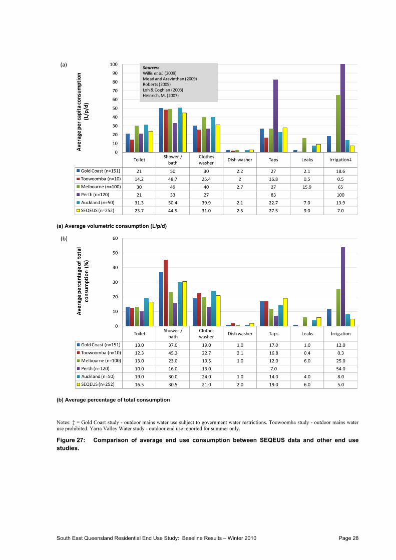
Average total per capita water use for the period of analysis reported by the QWC (2010) is presented below, together with the totals from the SEQEUS (Table 6). It can be seen from this table that there are some disparities between the two datasets. The reasons for the differences have been briefly discussed above. The method of calculation (underlying assumption of commercial/residential water use split) and the coarser bulk water demand data that is used by the QWC may slightly overestimate residential water use in SEQ. Conversely, the SEQEUS data may slightly underestimate average water use in SEQ due to possible biases in the sample, including: household occupancy rates; expected low representation of the very high water uses; and the lack of inclusion of multi-unit dwellings. These dwelling types are not included in the present study. Additionally, it has been observed that householders are more likely to use less water if they are aware of being monitored (e.g. Stewart et al. 2010) and this may be occurring to some extent in this study. It is anticipated that this phenomenon will play less of a role as the awareness diminishes. Notwithstanding the differences, the trend for Ipswich to use less water and the Sunshine Coast to use more water has been captured in both datasets. Furthermore, Brisbane averages are very similar, with only a 4 L/p/d difference over the period.

Table 6: Comparison of average total per capita water use (L/p/d) for dwellings in SEQ.

Data Source Gold Coast Brisbane Ipswich Sunshine Coast

QWC 18th June 183 138 138 189

QWC 25th June 180 142 142 185

QWC period average 182 140 140 187

SEQEUS 14 to 24th June 141 144 111 171

In terms of irrigation, properties located in the Gold Coast used slightly, but not significantly, more than the other regions. This is interesting as this region, along with the Sunshine Coast, received the most rainfall during the period of analysis (Table 3). Ipswich used the least water for irrigation yet had the driest weather of all regions during June (Table 3). Some conclusions may be drawn from this observation. After recent wet periods, residents may feel less restricted or guilty in using water to irrigate the garden. As a final note, the average irrigation volumes and total volumes in general are substantially lower than those from a decade earlier.

Temperature rather than rainfall may be a stronger trigger for irrigation and this will be measured and reported on with the summer end use analysis results (December 2010). The garden size of homes in the Sunshine and Gold Coasts may be generally larger than those of Ipswich and Brisbane, thus using more water, although this information is not able to be readily determined at this stage. Soil texture and moisture holding capacity of soils will also determine the frequency and volume of irrigation. Soil characteristics vary across SEQ, however the predominant upper horizon soils (e.g. Kurosols)

Brisbane Gold Coast Sunshine Coast Ipswich

Irrigation 5.0 6.7 4.0 1.5

Bathtub 1.2 1.4 1.7 0.0

Tap 15.8 24.3 15.6 20.7

Dish washer 1.6 1.1 2.5 1.3

Shower 26.9 29.0 29.9 32.6

Clothes Washer 24.9 19.8 19.9 22.0

Toilet 15.3 14.6 18.2 19.2

Leak 9.3 3.1 8.2 2.6

0

25

50

75

100

Average percentage of total

water consumption (%)


typically have a low moisture holding capacity in the Brisbane and Ipswich regions and a slightly higher capacity (especially in the elevated regions, e.g. Red Ferrosols) in the coastal councils. Finally, the increased use of stored rainwater from tanks for external purposes may also contribute to the lower irrigation end uses from mains water. This final point is explored more in Section 4.6.

4.3.2. Gold Coast

Properties in the Gold Coast recorded an average total water consumption of 347.5 L/hh/d or 140.8 L/p/d (Figure 22a), ranging from 26 L/p/d to 549 L/p/d (Figure 22b). End use break down on a per capita basis indicates that, on average, shower (29 %), tap (24 %) and clothes washer (20 %) comprised the bulk of the water consumption (Figure 22a). Irrigation contributed an average of 9.4 L/p/d or 7 % of total water use. The homes that used the most water had a disproportionately high contribution from irrigation (Figure 22b). This is consistent across all regions examined. Water used for clothes washing and showers was markedly varied across the sample and may reflect the mix of household types (single, family, pensioners) that were present in this region. Data from Table 2 suggests that both small and large families with young children were fairly evenly represented compared to the other regions.

(a) Per capita end use break down (L/p/d) (b) Per capita end use break down (L/p/d) by household

Figure 22: Break down of average end uses for the Gold Coast.

4.3.3. Brisbane

Average household consumption in Brisbane was 331.4 L/hh/d, resulting in a per capita consumption average of 143.8 L/p/d (Figure 23). End use break down on a per capita basis indicates that, once again, shower (26.9 %), clothes washer (24.9 %) and tap (15.8 %) comprised the bulk of the water consumption (Figure 23a), contributing over 65 % (97 L/p/d) of daily usage. There was an association between the number of young children in the home and clothes washing and showering. The Brisbane sample had the youngest average age of children (2.7 years) and the highest consumption for water resulting from clothes washing (Figure 21).

The Brisbane total amount of daily per capita usage attributed to leaks was the second highest across the regions at 13.3 L/p/d representing 9.3 % of total household water use (Figure 21 and Figure 23a). However, this result was skewed by extraordinarily high leak usage attributed to two homes, with one household showing average daily consumption from leaks at over 500 L/p/d (Figure 23b). For the average householder, the percentage attributed to leaks was much less at 4.4 L/p/d (3 % of total water use). It is necessary to include these high leak homes as they are not outliers, rather they represent a small number of homes (usually 3-5 % of dwelling stock) having very high leakage rates and this is typical of a ‘normal’ sample of households (Britton et al. 2009).

0

100

200

300

400

500

600

Household W


Household ID

Irrigation

Bathtub

Tap

Dishwasher

Shower

Clothes Washer

Toilet

Leak

(b)Leak4.3 L (3%)

Toilet 20.6 L (15%)

Clothes Washer

27.9 L (20%)

Shower 40.9 L (29%)Dish

washer1.6 L (1%)

Tap 34.2 L(24%)

Bathtub1.9 L (1%)

Irrigation9.4 L (7%)


(a)


Irrigation in the Brisbane region was 5 % of total daily usage, or 7.2 L/p/d. This figure was over-represented in some households (Figure 23b). It was noted during the analysis that people who reported that they irrigate their gardens usually did so using a constant and medium flow rate with the event lasting between 15 minutes to one hour on average.


Figure 23: Break down of average end uses for Brisbane.

4.3.4. Ipswich

The period of analysis in the Ipswich region showed an average household consumption of 305.4 L/hh/day. This resulted in a low per capita figure of 111.2 L/p/d (Figure 24a), nearly half of the QWC Permanent Water Conservation Measures target of 200 L/p/d. Per capita total water use ranged from 283 to 20 L/p/d (Figure 24b). The low per capita use (20 L/p/d) measured for one home was a result of frequent absences of the sole occupant of the property. In general, there was less variation in total household use in Ipswich than the other regions. For example, the standard deviation was 46 L/p/d for Ipswich, which is low when compared with the average standard deviation for the other regions of 90 L/p/d (Figure 25). This is unexpected given the smaller sample size for Ipswich and may suggest that water conservation and water use awareness is more uniform across all family types and socio-demographic groups in this region. This may also partly explain the low overall water use compared to the other regions. Further examination of water use patterns and socio-demographics in future reports will explore this more.


Figure 24: Break down of average end uses for Ipswich.

Leak 13.3 L/p/d(9.3%)

Toilet 22 Lp/d (15.3%)

Clothes Washer 35.8 L/p/d (24.9%)

Shower 38.6 L/p d (26.9%)

Dish washer 2.3 L/p/d(1.6%)

Tap 22.7 L/p/d (15.8%)

Bathtub 1.8 L/p/d (1.2%)

Irrigation 7.2 L/p/d (5%)


(a)

0

100

200

300

400

500

600

700

Household W


Household ID

Irrigation

Bathtub

Tap

Dishwasher

Shower

Clothes Washer

Toilet

Leak

(b)

Leak 2.9 L/p/d (3%)

Toilet 21.4 L/p/d (19%)

ClothesWasher 24.5

L/p/d (22%)Shower 36.3

L/p/d(33%)

Dish washer1.4 L/p/d (1%)

Tap 23 L/p/d(21%)

Irrigation 1.7 L/p/d (2%)


(a)

0

50

100

150

200

250

300

Household W


Household ID

Irrigation

Bathtub

Tap

Dishwasher

Shower

Clothes Washer

Toilet

Leak

(b)


Per capita analysis showed that showers (33 %), taps (21 %) and clothes washers (22 %) made up the bulk of individual water usages (Figure 24a), and contributed over 75 % (81 L/p/d) of daily usage. Toilet usage accounted for 19 % of average daily usage, or 21.5 L/p/d; this percentage is greater than other regions (Figure 21) and may be heightened by the relatively low total per capita daily water consumption for Ipswich. Daily bathtub usage was extremely low, less than 1 % across the Ipswich region; a reflection of the low percentage (21 %) of homes with children in the region (Table 2).

Figure 25: Standard deviation for individual end uses across the regions: comparing variance.

4.3.5. Sunshine Coast

The Sunshine Coast residents consumed the highest volumes of water for all regions, with an average household consumption of 472.2 L/hh/day, equating to an average daily per capita consumption of 170.8 L/p/d (Figure 26a). The biggest indoor water usages were attributed to showers 51.1 L/p/d (30 %), clothes washers 34 L/p/d (20 %) and toilets 31.1 L/p/d (18 %), which together resulted in daily consumption of 116 L/person, or 68 % of total daily per capita usage.

The Sunshine Coast sample had the oldest average age for children (10 years) and highest percentage of pensioners and retired residents (Table 2). There was more likely to be greater occupancy during the day in this region than compared to regions that had a lower daytime occupancy rate (e.g. Brisbane demographic are more likely to be working and attending school). During the analysis, it was regularly observed that the homes that were occupied by older residents tended to use more water for showers and toilets. This is confirmed by the high shower usage and relatively elevated toilet usage observed in Figure 26. Water loss attributed to leaks was the highest of all the regions at 14.1 L/p/d, with a small number of households having elevated leakage rates (Figure 26). However, in terms of percentages, leaks were lower than reported from Brisbane households (Figure 23).

0

20

40

60

80

100

Gold Coast Brisbane Ipswich Sunshine Coast

Standard deviation from the mean

(L/p/d)

SEQ Region

Leak

Toilet

Clothes Washer

Shower

Dishwasher

Tap

Bathtub

Irrigation

Total



Figure 26: Break down of average end uses for the Sunshine Coast.

4.4. End Use Comparisons with Similar Studies Volumetric consumption for all end uses fell within the range reported in other studies with the exception of irrigation (Figure 27a). At an average of 7 L/p/d, irrigation was noticeably lower for this study compared to the combined average 40 L/p/d reported in other studies. On a percentage basis, there was also good agreement between this and other end use studies, again with the noticeable exception of irrigation, i.e. 5 % for SEQEUS versus a combined average of 20 % for other studies (Figure 27b).

Some discussion on the low irrigation volumes observed in this study was undertaken in Section 4.3.1. Essentially, several factors are likely to be influencing the low irrigation volumes observed in this study. A lingering reluctance to use mains water outdoors as a result of the recent drought and an associated strong awareness of water conservation is one underlying factor. Another is related to seasonal factors, including the relatively frequent rainfall (days > 1 mm of rain) in SEQ leading up to the winter 2010 read, and much reduced need to irrigate during winter months to sustain grass and plant life. End use analysis during summer months should reveal to what extent households are willing to irrigate to sustain plant and grass life.

As for previous studies, shower usage comprised the bulk of household water use for all regions. Across all regions, a minimum of one quarter of all household water demand was associated with this practice. This is not unusual and has been reported in other end use studies (Willis et al. 2009b, Mead and Aravinthan 2009, Roberts 2005).

Leakage rates for the SEQEUS are, in terms of percentage of total water consumption, slightly higher than the average, although within the mean standard deviation. Leaks are a common occurrence in all households, with a trend typically shown for less leakage to occur from new (< 5 years old) dwellings (Willis et al. 2009a). For the SEQEUS sample, leaks ranged from 0.2 to 513L/p/d. The latter value is an extreme case and subsequent investigation has revealed that this household has had ongoing issues with leaks on its property. Very large leaks are usually due to service breaks and can cause the average per capita leakage volumes in an end use sample to fluctuate significantly. The forthcoming summer read will serve to develop a more representative average household or per capita leakage volume.

Leak 14.1 L/p/d(8%)

Toilet 31.1 L/p/d(18%)

Clothes Washer34 L/p/d(20%)

Shower51.1 L/p/d(30%)

Dish washer4.2

L/p/d(3%)

Tap 26.6 L/p/d16%

Bathtub2.9 L/p/d (2%)

Irrigation6.8 L/p/d (4%)


(a)

0

100

200

300

400

500

600

700

Household W


Household ID

Irrigation

Bathtub

Tap

Dish washer

Shower

Clothes Washer

Toilet

Leak

(b)


ToiletShower /

bath

Clothes

washerDish washer Taps Leaks Irrigation‡

Gold Coast (n=151) 21 50 30 2.2 27 2.1 18.6

Toowoomba (n=10) 14.2 48.7 25.4 2 16.8 0.5 0.5

Melbourne (n=100) 30 49 40 2.7 27 15.9 65

Perth (n=120) 21 33 27 83 100

Auckland (n=50) 31.3 50.4 39.9 2.1 22.7 7.0 13.9

SEQEUS (n=252) 23.7 44.5 31.0 2.5 27.5 9.0 7.0

0

10

20

30

40

50

60

70

80

90

100

Average per capita consumption

(L/p/d)

Sources: Willis et al. (2009)Mead and Aravinthan (2009)Roberts (2005)Loh & Coghlan (2003)Heinrich, M. (2007)

(a)

(a) Average volumetric consumption (L/p/d)

ToiletShower /

bath

Clothes

washerDish washer Taps Leaks Irrigation

Gold Coast (n=151) 13.0 37.0 19.0 1.0 17.0 1.0 12.0

Toowoomba (n=10) 12.3 45.2 22.7 2.1 16.8 0.4 0.3

Melbourne (n=100) 13.0 23.0 19.5 1.0 12.0 6.0 25.0

Perth (n=120) 10.0 16.0 13.0 7.0 54.0

Auckland (n=50) 19.0 30.0 24.0 1.0 14.0 4.0 8.0

SEQEUS (n=252) 16.5 30.5 21.0 2.0 19.0 6.0 5.0

0

10

20

30

40

50

60


consumption (%)

(b)

(b) Average percentage of total consumption

Notes: ‡ = Gold Coast study - outdoor mains water use subject to government water restrictions. Toowoomba study - outdoor mains water use prohibited. Yarra Valley Water study - outdoor end use reported for summer only.

Figure 27: Comparison of average end use consumption between SEQEUS data and other end use studies.


4.5. Diurnal Patterns of Water End Use Consumption Diurnal patterns can be used to characterise patterns of water use across different climatic regions and socio-demographic groups. Diurnal pattern data of water end uses were generated for each region (Figures 28 to 31). These graphs provide a representation on the average day and hour flow rates (on a per capita basis) for the residential detached households in the sample. The average peak (and low) periods of water demand can be determined on a real-time basis, providing valuable information for water utilities to address a range of engineering, planning, billing and asset management functions including: (1) understanding the required supply quantities throughout day; (2) better knowledge of reservoir storage needs; (3) better data on discharge volumes (and potentially their constituents) at particular times; (4) refining water distribution network model diurnal demand parameters thereby enabling optimised pump and pipe infrastructure design and planning and ultimately improved capital efficiency; and (5) identify end uses contributing to peak demand, thereby understanding how to influence change through water demand management policies. In summary, the development of a repository of end use diurnal pattern curves for average and peak days and different classifications of users (e.g. single detached, multi-unit, commercial, industrial, etc.) is essential for the optimised management of urban water in the future.

4.5.1. Gold Coast Diurnal Pattern Analysis

Diurnal pattern analysis on the Gold Coast demonstrates the morning peak of around 14 litres per person per hour per day (L/p/h/d) between 8 and 9 am is higher and sharper than the afternoon peak of just under 8 L/p/h/d occurring over a longer period from around 5.30 to 7.30 pm (Figure 28). There is a clear and steady rise in water demand from 3.00 pm onwards which coincides with after school hours. Almost 50 % of the Gold Coast participants reported household incomes in the low to middle income range of between $30,000 and $90,000, which typically coincides with ‘8-to-5’ employment.

Figure 28: Average daily diurnal pattern analysis - Gold Coast sample.

1 2 3 4 5 6 7 8 9 10 11 12 13 14 15 16 17 18 19 20 21 22 23 24

Irrigation 0.00 0.00 0.02 0.00 0.03 0.07 0.28 0.77 0.44 0.34 0.38 1.07 0.11 0.66 0.51 0.94 1.00 1.35 0.39 0.23 0.07 0.03 0.03 0.00

Shower 0.27 0.13 0.20 0.30 0.28 1.94 3.95 4.25 4.03 3.12 2.35 1.68 0.91 1.04 0.76 1.48 1.75 2.92 2.72 1.98 1.57 0.99 0.88 0.19

Clothes Washer 0.00 0.00 0.00 0.03 0.04 0.13 1.08 2.34 4.05 3.69 2.33 1.64 1.97 1.38 1.08 0.94 1.26 1.04 1.10 0.65 0.42 0.33 0.25 0.06

Toilet 0.16 0.16 0.09 0.19 0.44 0.64 1.37 1.86 1.48 1.21 0.87 0.80 0.86 0.76 0.79 0.93 1.02 1.04 1.24 1.12 0.94 0.85 0.70 0.39

Tap 0.15 0.10 0.07 0.11 0.29 0.75 1.83 2.76 2.80 2.24 1.77 1.45 1.43 1.24 1.30 1.36 1.80 2.15 2.42 1.95 1.40 1.24 1.02 0.37

Bathtub 0.00 0.00 0.00 0.00 0.00 0.00 0.00 0.39 0.27 0.28 0.27 0.11 0.04 0.02 0.00 0.04 0.20 0.37 0.55 0.15 0.02 0.08 0.02 0.00

Dishwasher 0.04 0.00 0.00 0.00 0.00 0.01 0.03 0.11 0.16 0.17 0.08 0.03 0.06 0.07 0.07 0.05 0.05 0.06 0.17 0.19 0.15 0.13 0.05 0.06

Leak 0.34 0.31 0.34 0.25 0.29 0.42 0.34 0.45 0.70 0.36 0.36 0.35 0.26 0.44 0.36 0.86 0.51 0.38 0.59 0.42 0.47 0.46 0.40 0.20

0

2

4

6

8

10

12

14

Average

daily diurnal consumption (L/p/h/d)

Time (0:00 hours)


The flattened morning period for tap and toilet usage also reflects the Gold Coast having the largest percentage of homes with children (34 %). Consistent tap and toilet usage for the entire day suggest a large percentage of households see one or more occupants remain at home all day. Clothes washer usage is also concentrated in the 8 am-2 pm period (Figure 28) suggesting that washing is conducted in the middle of the day to take advantage of the afternoon sun. There appeared to be a temporal trend between water usage via leaks and toilet use, suggesting that toilet fixtures are a key source of leaks within this sample. This relationship is explored further in Section 5.5.7.

An interesting note is that the bulk of irrigation events in the Gold Coast took place within the 11 am – 5 pm period of the day, despite QWC permanent water restriction measures prohibiting irrigation between the hours of 10 am and 4 pm. However, the peak irrigation times were outside these hours.

4.5.2. Brisbane Diurnal Pattern Analysis

The diurnal pattern for Brisbane shows the typical morning peak and smaller afternoon peak, but also a minor peak in the early afternoon for shower, clothes washer and irrigation (Figure 29). The Brisbane sample had the highest number of homes with children, and the youngest average age of children and this may be represented by the early afternoon peak where one adult and one or more small children are at home during the day. Water demanding activities such as clothes washing and showering are more likely to occur during the day for these people than in the morning or evening where other activities would be occurring (e.g. meal preparation, morning outings, etc.).

Figure 29: Average daily diurnal pattern analysis - Brisbane Region.

1 2 3 4 5 6 7 8 9 10 11 12 13 14 15 16 17 18 19 20 21 22 23 24

Irrigation 0.04 0.00 0.00 0.03 0.00 0.00 0.00 1.27 0.05 0.59 0.33 0.40 0.21 0.42 0.21 0.42 0.73 0.35 0.09 0.38 0.18 0.12 0.16 0.09

Shower 0.31 0.10 0.00 0.00 0.08 1.13 4.07 3.96 4.47 3.10 2.04 1.38 1.06 0.98 0.72 0.89 2.00 3.02 3.30 2.58 1.61 2.42 1.64 0.88

Clothes Washer 0.11 0.00 0.02 0.00 0.04 0.24 1.21 2.87 4.01 5.27 4.10 3.40 2.36 2.62 1.68 2.17 1.97 1.49 1.62 1.56 0.92 0.34 0.16 0.25

Toilet 0.23 0.22 0.18 0.12 0.19 0.51 1.42 1.78 1.52 1.16 1.06 0.91 0.90 1.01 1.00 1.04 1.19 1.34 1.26 1.42 1.14 1.16 0.82 0.47

Tap 0.11 0.07 0.04 0.02 0.13 0.39 1.10 1.55 1.79 1.61 1.27 1.23 1.10 1.04 1.04 1.19 1.21 1.72 2.25 1.38 1.10 0.84 0.71 0.36

Bathtub 0.00 0.00 0.00 0.00 0.00 0.00 0.18 0.05 0.05 0.13 0.08 0.06 0.02 0.05 0.19 0.04 0.30 0.73 0.51 0.12 0.12 0.01 0.06 0.01

Dishwasher 0.00 0.00 0.00 0.00 0.00 0.01 0.07 0.14 0.22 0.14 0.14 0.11 0.12 0.14 0.13 0.08 0.11 0.19 0.29 0.49 0.30 0.24 0.17 0.02

Leak 0.12 0.11 0.10 0.10 0.10 0.12 0.15 0.17 0.18 0.16 0.16 0.16 0.19 0.16 0.17 0.18 0.18 0.18 0.18 0.17 0.17 0.15 0.15 0.14

0

2

4

6

8

10

12

14

Average

daily diurnal consumption (L/p/h/d

)

Time (0:00 hours)


4.5.3. Ipswich Diurnal Pattern Analysis

The Ipswich region showed distinct double peaks in the diurnal usage analysis for both morning and the evening periods (Figure 30). In particular, the peaks contain sharp concentrations of shower and tap usages. The double peaks suggest that there may be two clear family types; a smaller household leaving early and returning later from work, and a larger, younger family where school age children leave the house later in the mornings and return home earlier in the evenings.

Figure 30: Average daily diurnal pattern analysis - Ipswich Region.

Ipswich householders with families had relatively young children at an average age of 4.4 years old, suggesting that the children shower earlier at distinctly different times to the adults. About 50 % of households in Ipswich had two or fewer occupants. During the trace analysis it was observed that these two-person households were typically younger, and appeared to spend more time away from the household, leaving for work earlier and returning home later. This absence from the home during the day is reflected in the deep trough in the middle of the day in Figure 30.

4.5.4. Sunshine Coast Diurnal Pattern Analysis

Diurnal pattern analysis of the Sunshine Coast region shows two distinct peaks, at 9 am and again around 6 pm (Figure 31). The sharp peaks show a high concentration of shower events, which correlates with the 69 % of households in the region being occupied by 2 or fewer occupants (Table 2), resulting in less of a time spread than larger households. The analysis also shows a consistent pattern of shower, toilet and tap events throughout the day, which is typical of older families, who tend to remain at home more than younger households. Leakage rates in the morning peak were dominated by one home.

1 2 3 4 5 6 7 8 9 10 11 12 13 14 15 16 17 18 19 20 21 22 23 24

Irrigation 0.00 0.00 0.00 0.00 0.00 0.00 0.16 0.00 0.14 0.00 0.07 0.77 0.00 0.00 0.00 0.00 0.28 0.25 0.08 0.00 0.00 0.73 0.00 0.00

Shower 0.36 0.29 0.00 0.00 0.20 0.93 3.34 3.53 2.50 3.27 1.85 1.57 1.05 1.20 0.79 1.37 3.22 4.00 2.20 2.89 1.59 1.71 0.92 0.42

Clothes Washer 0.04 0.02 0.02 0.03 0.08 0.01 0.67 2.51 2.74 2.52 2.64 2.71 1.44 0.66 1.02 1.15 1.22 0.92 0.89 0.63 0.78 0.44 0.19 0.17

Toilet 0.25 0.26 0.24 0.18 0.40 0.57 1.02 1.53 1.50 1.18 0.92 0.85 0.93 0.94 0.85 1.06 1.10 1.23 1.32 1.20 1.22 1.03 0.73 0.46

Tap 0.18 0.15 0.10 0.09 0.27 0.25 0.64 1.31 1.31 1.79 2.10 1.44 0.97 0.80 1.24 0.84 1.14 1.29 1.37 1.33 0.87 0.52 0.38 0.31

Bathtub 0.00 0.00 0.00 0.00 0.00 0.00 0.00 0.00 0.00 0.00 0.00 0.00 0.00 0.03 0.00 0.00 0.00 0.03 0.02 0.00 0.00 0.00 0.00 0.00

Dishwasher 0.01 0.03 0.02 0.00 0.02 0.01 0.05 0.10 0.12 0.10 0.08 0.08 0.07 0.05 0.09 0.10 0.06 0.16 0.27 0.20 0.12 0.08 0.04 0.01

Leak 0.11 0.11 0.12 0.11 0.11 0.12 0.13 0.16 0.15 0.13 0.12 0.12 0.12 0.12 0.13 0.13 0.12 0.13 0.13 0.15 0.15 0.17 0.12 0.12

0

1

2

3

4

5

6

7

8

9

10

Average


Time (0:00 hours)


Figure 31: Average daily diurnal pattern analysis - Sunshine Coast Region.

4.5.5. SEQ Diurnal Pattern Analysis

The combined average day diurnal patterns are shown in Figure 32. The major contributors to the peak water use periods of 7 am to 10 am were shower, toilet and clothes washer. Similarly, the major contributors to the afternoon period of 5 pm to 8 pm were shower and toilet, with tap use typically peaking more during this afternoon period. All of the regions demonstrated a concentration of washing machine use in the 9 am to 12 pm period. In general, the restrictions on daytime irrigation appear to be adhered to, with the peak times occurring outside these hours, although some irrigation was occurring throughout the day in all regions. Shower use was typically heightened in the morning between 6 am and 10 am, although, as would be expected, tap use occurred fairly evenly throughout the day. Water use for baths is predominantly occurring in the evening and it is likely to be over represented by younger families.

1 2 3 4 5 6 7 8 9 10 11 12 13 14 15 16 17 18 19 20 21 22 23 24

Irrigation 0.07 0.01 0.01 0.03 0.06 0.15 0.48 0.94 1.68 2.05 1.28 0.46 0.39 0.48 0.40 0.34 0.28 0.41 0.43 0.23 0.12 0.20 0.09 0.07

Shower 0.06 0.03 0.00 0.03 0.00 1.03 4.98 4.11 5.40 3.97 3.74 2.70 2.39 1.34 1.47 1.75 2.06 4.54 3.38 3.21 2.13 2.16 1.77 0.54

Clothes Washer 0.86 0.74 0.47 0.39 0.47 0.53 0.84 1.23 1.52 1.82 1.39 1.55 1.04 1.54 2.14 2.10 1.52 0.96 1.51 1.83 0.99 1.15 1.28 0.88

Toilet 0.40 0.26 0.18 0.18 0.33 0.71 1.66 2.46 2.09 1.70 1.36 1.23 1.21 1.22 1.25 1.40 1.52 1.73 1.68 1.59 1.46 1.30 1.17 0.69

Tap 0.21 0.14 0.06 0.08 0.15 0.36 1.09 2.07 2.12 1.92 1.35 1.32 1.35 1.11 1.03 1.58 1.32 1.91 2.17 1.43 1.27 0.92 0.77 0.38

Bathtub 0.08 0.02 0.00 0.00 0.01 0.00 0.03 0.05 0.09 0.16 0.10 0.08 0.07 0.08 0.08 0.07 0.04 0.07 0.11 0.14 0.15 0.14 0.12 0.09

Dishwasher 0.01 0.00 0.00 0.00 0.00 0.02 0.03 0.04 0.06 0.13 0.12 0.10 0.07 0.06 0.03 0.19 0.16 0.44 0.56 0.25 0.22 0.04 0.03 0.07

Leak 0.01 0.00 0.00 0.00 0.02 0.18 0.49 1.26 1.98 2.38 2.12 1.42 1.27 0.56 0.36 0.51 0.45 0.39 0.22 0.22 0.15 0.24 0.15 0.08

0

2

4

6

8

10

12

14

16

Average


Time (0:00 hours)


Figure 32: Cumulative average daily diurnal pattern analysis – SEQ sample (all regions).

4.5.6. Average Peak Day Total Consumption

The peak water use as an average for all the regions is shown in Figure 33 where the greatest concentration of water consumption is during the morning. The average maximum peak of 12 L/p/h/d occurred at 9.00 am and the secondary afternoon peak occurred at 6 pm at an average of approximately 9 L/p/h/d (Figure 33).

Figure 33: Average daily diurnal peak water use – Average for all regions, winter 2010.

1 2 3 4 5 6 7 8 9 10 11 12 13 14 15 16 17 18 19 20 21 22 23 24

Brisbane 0.9 0.5 0.3 0.3 0.5 2.3 7.8 11.2 11.7 11.5 8.7 7.2 5.6 6.1 4.9 5.7 7.3 8.5 9.0 7.7 5.3 5.0 3.7 2.1

Sunshine Coast 1.7 1.2 0.7 0.7 1.0 3.0 9.6 12.2 14.9 14.1 11.5 8.8 7.8 6.4 6.8 7.9 7.3 10.4 10.1 8.9 6.5 6.1 5.4 2.8

Gold Coast 0.9 0.7 0.7 0.8 1.3 3.8 8.5 12.4 13.4 11.0 8.1 6.8 5.4 5.4 4.7 6.3 7.3 8.9 8.8 6.4 4.8 3.9 3.2 1.2

Ipswich 0.9 0.9 0.5 0.4 1.1 1.9 6.0 9.1 8.5 9.0 7.8 7.5 4.6 3.8 4.1 4.6 7.1 8.0 6.3 6.4 4.7 4.7 2.4 1.5

0

5

10

15

20

25

30

35

40

45

50Average daily diurnal consumption (L/p/h/d)

Time (0:00 hours)

0

3

6

9

12

1 2 3 4 5 6 7 8 9 10 11 12 13 14 15 16 17 18 19 20 21 22 23 24

Average


Time (0:00 hours)


As the data in Figure 33 is for the average day for the winter 2010 period, there is likely to be a shift slightly during the summer months and if daylight savings was to occur. Peak water use data can be used to compare weekdays to weekends, compare seasonal differences (where irrigation is typically greater in the summer) and also to determine peak hourly and daily consumption for specific occasions where water demand is extreme. For example, trace analysis can be conducted on the sample for peak events of the year (such as Boxing Day and Australia Day) which will establish a ‘peak hour’ and ‘peak day’ total consumption. This data is critical for many design parameters for pump and pipe infrastructure modelling, future network distribution planning and targeted demand management policy. Therefore, using diurnal pattern analysis and determining peak flow rates and times enables the establishment of a repository of patterns to inform design, planning and demand management policy.

4.5.7. Diurnal Relationships between End Uses

This section briefly explores end uses that are strongly correlated with each other in terms of diurnal usage. For example, as would be expected, tap and toilet end uses occur around the same time (Figure 34a). Shower use is also closely related to tap and toilet use (Figures 34b and 34d), all of which peak in the mornings.

R² = 0.878

0

0.5

1

1.5

2

2.5

3

0 1 2 3 4

Toilet (L/p/h/d)

Tap (L/p/h/d)

(a)

(a) Diurnal relationship between toilet and tap

R² = 0.762

0

1

2

3

4

5

6

7

0 1 2 3 4

Shower (L/p/h/d)

Tap (L/p/h/d)

(b)

(b) Diurnal relationship between shower and tap

R² = 0.4546

0

0.5

1

1.5

2

2.5

3

0.00 0.20 0.40 0.60 0.80

Toilet (L/p/h/d)

Leak (L/p/h/d)

(c)

(c) Diurnal relationship between toilet and leak

R² = 0.8251

0

1

2

3

4

5

6

7

0 1 2 3

Shower (L/p/h/d)

Toilet (L/p/h/d)

(d)

(d) Diurnal relationship between toilet and shower

Figure 34: Average diurnal relationship between end uses.

This confirms the belief that the morning ablution ‘rituals’ consume the major proportion of peak water use and occur consistently across all households and regions. Closer examination of the data could reveal that certain household types (i.e. where family members work or attend school regularly) might be overrepresented in this. Knowledge of this type can greatly assist water demand managers in implementing strategies to change water use behaviours, which may subsequently shift or flatten the peak usage times in these households.


Interestingly, the greatest association for leaks was with toilet usage (Figure 34c). There was a reasonably strong positive correlation between leakage and toilet water consumption end uses for all regions. During the water audits and trace analysis, it was clear that many of the leaks were attributable to toilets and in some instances leaks comprised almost 50 % of total water use. This is an area also worthy of further investigation, as, while we may have addressed the low flush dual toilet question, it may now be prudent to promote maintenance and inspection on these toilet fixtures.

4.6. End Use and Water Appliance Efficiencies Previous studies have shown associations between water efficient appliances and fixtures and reduced water demand in homes (Willis et al. 2009b, Heinrich 2008, Arthuraliya et al. 2008, Mayer et al. 2004).

The variation in clothes washing between homes is likely a reflection of the different types and models of appliances that are available. The stock surveys undertaken for each home revealed a variety of water star rating machines, with a clear trend for higher star rating machines to use less water (Table 7). Turner et al. (2009) and Willis et al. (2009b) both discussed the variation in end use water consumption as a result of efficient devices and Willis et al. (2009b) demonstrated that substantial water savings could be made by using high efficiency washing machines. Similarly, front loading machines used significantly less water (p<0.05) than top loaders and a significantly (p<0.05) lower proportion of total household water was required by front loading machines (Table 7). Estimated annual savings from water efficient washing machines (front loaders in particular) ranged from 2.5 to 4 kilolitres per person annum (kL/p/a) or around 7 to 11 kilolitres per household per annum (kL/hh/a). Results demonstrate that the installation of high water efficiency washing machines could save around 7 % of total household consumption.

Table 7: Clothes washer efficiency comparisons.

Clothes Washer Efficiency Clusters Description

Efficiency Rating Loading Type

Efficiency Feature ≤ 3 star ≥ 4 star Top Front

Daily per capita washing consumption (L/p/d)

35.1 28.3 33.8 22.5

Daily household washing consumption (L/hh/d)

94.7 76.4 91.2 60.7

Annual per capita washing consumption (kL/p/a)

12.8 10.3 12.3 8.2

Annual household washing consumption (kL/hh/a)

34.6 27.9 33.3 22.2

Low flow shower heads are another popular water efficient device that has been widely adopted in the last five years or so (Turner et al. 2007). Measured shower flow rates from each home were clustered into three efficiency categories that corresponded to the Water Efficiency Labelling Scheme (WELS) definitions, where low or standard non-efficient heads use 15 to 25+ litres per minute (L/min), medium shower heads consume 9 to 15 L/min and high efficiency shower heads can use less than 7 L/min. The clusters were based on average shower flow rates measured in the home, typically there was not a great deal of variation within homes where two or more showers were present. Results presented in Table 8 demonstrate the trend toward lower water consumption on a per capita and per household basis when high efficiency showerheads are installed.

Results show that replacing low efficient showerheads with high efficiency showerheads could provide household savings of 13 kL (or 26 %) per year. This is lower than reported by Willis et al. (2009b), however the percentage of householders that reported to have high efficiency/low flow showerheads in this study was over 70 %. Additionally, shower consumption for this study was lower than several of the previous studies (Figure 27) including Willis et al. (2009b), suggesting that the margin for savings will be less as the technology has already been widely adopted in the SEQEUS sample.


Table 8: Showerhead efficiencies cluster comparisons.

Description Shower Head Efficiency Clusters

Efficiency Rating (WELS rating) Low (A)

Medium (AA)

High (AAA)

Daily per capita shower consumption (L/p/d) 49.7 37.7 35.8

Daily household shower consumption (L/hh/d) 139.9 106.7 104.1

Annual per capita shower consumption (kL/p/a) 18.1 14.1 13.1

Annual household shower consumption (kL/hh/a) 51.1 39.0 38.0

Following the State and local government rebate schemes in the mid 2000s, around 240,000 homes in Queensland installed a rainwater tank. In this particular study, rainwater tanks (RWT) are installed in about 44 % (n=22) of Gold Coast homes, 48 % (n=29) of Brisbane homes, 65 % (n=24) of Ipswich homes and 25 % (n=17) of Sunshine Coast homes. Of these homes with a RWT, about 60 % stated during the water audit that they typically used their rainwater for outdoor garden watering. Other common uses were car washing and topping up pools. There was a slight positive correlation between irrigation and total end use consumption for homes without RWT. This is what we would expect as homes without RWT would irrigate more using mains water supplies. When assessed on a region by region basis there are obvious increases in irrigation by homes without RWT for Ipswich and Sunshine Coast, although this tendency is not appearing for the Gold Coast and Brisbane (Figure 35). Similarly, the proportion of total water consumed for irrigation (or other external uses) for homes without RWT is also higher for Ipswich and the Sunshine Coast. This demonstrates that there are some mains water savings to be made by the installation of non-internally plumbed RWT, although this may be more clearly seen in the warmer summer months when irrigation is more prevalent, and tank use capacity is maximised from more frequent rainfall.

0

1

2

3

4

5

6

7

8

9

10


Average w

ater consumed

from irrigation (L/p/d)

Homes with RWT

Homes without RWT(a)

(a) Irrigation end use per capita volume

0

1

2

3

4

5

6

7

8



water use used fo

r irrigation (%)

Homes with RWT

Homes without RWT(b)

(b) Irrigation percentage of total use

Figure 35: Irrigation end use consumption for households with and without RWT.

The above, and other, relationships between water efficient appliances and end uses will be explored more thoroughly in a forthcoming report, specifically addressing these aspects, in order to form some evidence-based recommendations that can be utilised to inform water demand management policy.

4.7. End Use Patterns and Socio-Demographics Water consumption has been shown to be influenced by some key socio-demographic factors: household income, household occupancy and house size (Renwick and Archibald 1998, Kim et al. 2007, Turner et al. 2009). This section briefly explores the effect of several socio-demographic factors on water use for the SEQEUS sample. There will be a more detailed examination of these relationships in future reports and papers.


4.7.1. Income and Household Resident Typology

The relationship between income categories, people per household and total water usage on a per capita basis is demonstrated in Figure 36. Previous studies such as Kim et al. (2007) and Kenney et al. (2008) have reported a higher water consumption per capita for larger, higher-income homes although this was not observed in this study. Data in Figure 36 shows a trend for higher income families to have larger households but use relatively less water than lower-income, smaller families. This may reflect the likelihood of the occupants of a higher income household to be away from home for greater periods, when compared to low income groups such as single parent families and pensioners. Willis et al. (2009b) found no significant differences between water consumption across four different socio-economic groups although the higher-income group used the least volume of water during the period of analysis. Willis et al. (2009b) suggested that the higher socio-economic households would be more likely to purchase water efficient appliances such as washing machines and dishwashers. Leakage volumes may also be lower in these socio-economic groups. These relationships will be explored in depth in the summer end use analysis and reported in subsequent technical reports.

The average age is also shown on the bar plots of each income category in Figure 36. There is a noticeable trend for older households to use more water. Willis et al. (2009b) has reported that retired couples tend to use more water per capita and this may be due to medical requirements, increased toilet flushing, and increased presence in the home throughout the day. Conversely, younger households were observed to use less water per capita, despite the households being typically larger. This coincided with higher household incomes also, where the factors of higher efficiency appliances, potentially greater conservation awareness, and less time in the home may also be at play.

Figure 36: Relationship between income category, age and average household occupancy.

There was an expected trend towards higher household water use as household occupancy rates increased (Figure 37) as also reported by others (e.g. Turner et al. 2009, Willis et al. 2009a). Typically, water consumption will be higher for large homes with large families as the demand for water is obviously greater and there are a higher number of water fixtures and appliances (e.g. 2+ toilets, 2+ bathrooms/showers). Paradoxically, larger families are usually more water efficient on a per capita basis due to economies of scale (Turner et al. 2009, Russell and Fielding 2010). This trend is generally shown for the SEQEUS sample (Figure 37), although as only a small number of households had an occupancy of 6 or more, the trend is not strongly shown (less reliable) for these larger families.

0.0

0.5

1.0

1.5

2.0

2.5

3.0

3.5

0

20

40

60

80

100

120

140

160

180

< 30 30 ‐ 59 60 ‐ 89 90 ‐ 119 120 ‐ 149 >150 Prefer not to respond

Average

people per household

per income category

Average

total household w

ater

consumption (L/p/d)

Household income category ($ '000)

Per capita water use (LHS) Average age (years) Persons per household (RHS)

65

5042444347

54


Figure 37: Water consumption efficiency on per capita and per household basis.

End use comparisons were also made between different household typologies. Households were grouped into single (1 person), adult household (2 people), small family (e.g. 2 adults and 1 child), medium family (e.g. 2 adults and 2 children) and large family (5 or more people). Comparing trends between per capita (Figure 38) and per household (Figure 39) again shows that larger families are typically more water efficient on a per capita basis. The water consumption pattern for a single household shows a relatively even consumption across all end uses with a growing trend for higher clothes washer, shower and tap use as the households become larger. Bathtub use is also apparent mainly in the households with families. The high leakage for single households is likely to be influenced by an extreme leak event for one single household recorded in Brisbane. Multivariate analysis will be conducted to see if there is any predictive relationship between end use consumption and household typology. These results will be presented in future reports.

Figure 38: Per capita water consumption for different household typologies.

0

200

400

600

800

1000

1200

0

20

40

60

80

100

120

140

160

180

200

1 2 3 4 5 6 7 8

Average total daily household use (L/hh/d)

Average total daily per capita use (L/p/d)

People per household

Daily per capita use (LHS)

Daily per household use (RHS)

(n=39) (n=3) (n=1) (n=1)(n=13)(n=37)(n=49)(n=109)

Single

household

Adult

household Small family Medium family Large family

Irrigation 34.6 35.7 34.9 27.1 30.0

Bathtub 0.6 1.4 3.5 3.0 0.8

Tap 25.5 22.0 17.1 16.7 11.8

Dishwasher 7.0 10.2 5.6 5.9 6.9

Shower 32.0 27.6 36.5 24.6 28.1

Clothes Washer 26.9 30.9 35.0 28.2 32.7

Toilet 31.6 25.2 21.3 16.4 13.8

Leak 32.5 9.9 11.8 13.2 12.1

0

20

40

60

80

100

120

140

160

180

200

Average per capita

water comsumption (L/p/d)


Figure 39: Per household consumption for different household typologies.

4.7.2. Actual Versus Perceived Water Use Behaviours

As part of the Systematic Social Analysis study, an Alliance project running concurrently and in close collaboration with the End Use Study, each participant completed a detailed household water use survey. In this, participants were asked to identify whether they thought they were low, medium or high water users. These responses have been matched with the actual water use recorded as shown in Figure 40. Interestingly, only a small number of households (n=21) self-identified as being ‘low’ water users although their actual water use was 142 L/p/d, which was just under the average for the entire region. Following on from this, people who self-identified as ‘medium’ water users (n= 90) actually used more than the study average of 155 L/p/d and people who self-identified as ‘high’ water users (n=94) used the least at 130 L/p/d (Figure 40). The trend continued when analysing on a per household basis where the difference between ‘high’ and ‘medium’ water consumption was statistically different (p<0.05) at 465 L/hh/d compared with 295 L/hh/d, respectively (Figure 41).

The remaining respondents who answered ‘don’t know’ (n=17) had an average water use of 132 L/p/d. One implication of this is that water demand management policy cannot rely solely on individual household attitudes and beliefs to reduce water consumption. Mandatory measures such as water restrictions or incentives such as rainwater tank rebates are possibly more reliable in reducing residential demand, as has been shown in the past (Kenney et al. 2008, Renwick and Archibald, 1998).

The key end uses that were associated with the increased water use for ‘medium’ and ‘low’ water users were shower, clothes washer and toilet. Leakage rates were the greatest for the respondents who ‘didn’t know’ suggesting that they may have been aware of a leak but not sure its contribution to their total household water consumption.

Single household

Adult household

Small family Medium family Large family

Irrigation 34.6 71.3 104.6 108.3 134.9

Bathtub 0.6 2.8 10.4 12.1 3.6

Tap 25.5 44.1 51.2 66.8 53.0

Dishwasher 7.0 20.4 16.9 23.4 30.9

Shower 32.0 55.1 109.6 98.6 126.4

Clothes Washer 26.9 61.8 105.0 112.9 147.2

Toilet 31.6 50.4 64.0 65.5 62.0

Leak 32.5 19.7 35.5 52.6 54.3

0

100

200

300

400

500

600

Average per household

water comsumption (L/hh/d)


Figure 40: Comparisons of actual per capita water use with self-identified low, medium and high water users. Figure 41: Comparisons of actual household water use with self-identified low, medium and high water users.

"HIGH" "MEDIUM" "LOW" "DON'T KNOW"

Irrigation 4.2 7.6 8.2 4.5

Bathtub 1.5 2.6 1.7 0.8

Tap 25.7 28.4 25.3 24.8

Dish washer 2.1 3.4 2.5 1.4

Shower 33.0 49.1 43.0 37.6

Clothes Washer

26.6 34.2 34.8 24.1

Toilet 23.9 23.8 24.0 21.8

Leak 13.3 6.4 3.3 17.8

0

20

40

60

80

100

120

140

160

Households measured

water use (L/p/d)

Total 130 L/p/d

Total 155 L/p/d

Total

132 L/p/d

Total

142 L/p/d


Irrigation 8.7 14.6 18.9 10.7

Bathtub 3.7 8.8 6.4 1.6

Tap 55.2 79.2 64.3 55.9

Dish washer 5.0 9.6 6.7 3.9

Shower 82.4 157.3 119.3 97.9

Clothes Washer

62.5 108.5 97.3 53.2

Toilet 52.6 71.7 61.1 49.2

Leak 27.6 19.2 10.6 60.1

0

50

100

150

200

250

300

350

400

450

500

Households measured

water use (L/hh/d) Total

295 L/hh/d

Total

465 L/hh/d

Total 333 L/hh/d

Total 385 L/hh/d


In terms of household size and composition, there was some evidence to suggest that people with larger families underestimated their total water use (Figure 42). A significantly lower (p<0.05) household occupancy for ‘high’ water users compared to ‘medium’ users was detected (Figure 42a). Additionally, there were also significant differences (p<0.05) between the number of children in households that identified as ‘high’ users and the ‘medium and low’ users (Figure 42b). Therefore, people with larger families are tending to underestimate the contribution of children to household water demand. There may be a lack of knowledge of how and when children are using the household water.

0.0

0.5

1.0

1.5

2.0

2.5

3.0

3.5


Average number of peo

ple

per household

Householder's perceived water use

(a)

0.0

0.1

0.2

0.3

0.4

0.5

0.6

0.7

0.8

0.9


Average number of child

ren

per household


(b)

(a) Household size and perceived water use (b) Number of children and perceived water use

Figure 42: Selected family characteristics and self-identified low, medium and high water users. The ‘high’ water users fall in the lower household income category at an average income in the lower segment of the $60,000 to $90,000 bracket (Figure 43). Based on data presented in Figures 36 and 42, this group is likely to be older householders with smaller families.

Figure 43: Comparisons of income categories with self-identified low, medium and high water users.

0

1

2

3

4


Households total estimated

income (income factor)


< $30 K

$90 ‐ 119 K

$60 ‐ 89 K

$30 ‐ $59 K


In terms of water efficient appliances and fixtures there were some general trends for people who identified as low water users had higher star rated (Figure 44a) and water efficient (Figure 45a) clothes washers and lower flow rated shower heads (Figure 45b).

3.1

3.2

3.3

3.4

3.5

3.6

3.7


Average water efficiency star rating


(a)

0

25

50

75

100

"HIGH" "MEDIUM" "LOW "DON'T KNOW"

Porportion of top and front loading

clothes washers (%

)


Top Front(b)

(a) Machine star rating and perceived water use (b) Load type and perceived water use

Figure 44: Comparisons of washing machine efficiencies with self-identified low, medium and high water users. Although not significant (p>0.05), the group who identified as low water consumers had a greater percentage of top loading washing machines (Figure 44b), and while historically they are associated with higher water use per washing loads, the current range of top loaders can have high water efficiency ratings, although they are typically more expensive.

0

10

20

30

40

50

60

70

80

90


Average water efficiency for clothes

washer (L/wash)


(a)

0.140

0.145

0.150

0.155

0.160

0.165

0.170

0.175


Average shower flow rate (L/second)


(b)

(a) Water efficiency and perceived water use (b) Shower flow rate and perceived water use

Figure 45: Comparisons of washing machine and shower fixture water efficiencies with self-identified low, medium and high water users.


This data presented in this section suggests that households who have high incomes and water efficient appliance/fixture stock self-perceive they are lower overall users of water. This may result in these households being less concerned about the behaviourally influenced end uses such as showering and taps, thereby pushing their overall consumption higher. Syme et al. (2000) noted that people with water efficient appliances are not necessarily effective in saving water elsewhere in the house. Following on from this, family size and composition rather than the technology may be the greater factor in determining household water demand. That is, you can have good technology but also need to match this with water conserving behaviour for non-automated water fixtures (e.g. shower and taps).

The lack of feedback or education and awareness of how water is being used in the house may also be a factor in the water use perception not matching the water use behaviour. In this regard, the current intervention study that is being conducted by the SSA team will be examining the impact that interventions have on water use over time. One intervention is the provision of an end use pie chart to a sub-sample and this feedback on their water use may alter their initial perceptions on their household water use.


5. CONCLUSIONS AND POLICY CONSIDERATIONS

This section highlights some results from the report that may be useful to inform future policy directions for demand management. The relatively low water consumption reported for this study confirms the anecdotal and government reporting of a shift in general water consumption post drought in SEQ. This may be partly a result of the prolonged water restrictions that have created a behavioural shift in SEQ consumers. Given that the sample was across four regions of varying levels of water restrictions in the recent past (e.g. severe for Brisbane and Ipswich, more relaxed for the Gold and Sunshine Coasts) the observed trend of generally lower water consumption is likely to be representative across SEQ. This will be confirmed in future research linking end use data with consumer attitudinal data.

Gold Coast and Sunshine Coast were the highest water users and had the highest proportion of older, smaller families.

Clothes washing consistently contributed 20 % or more of total household water use. Elevated usage of clothes washers was generally associated with larger and younger families, and the older age brackets. This may be explained by the lower numbers of water efficient washing machines that were present in these older households. Conversely, large families with young children tended to have more efficient and updated models, therefore reducing the water demand for this end use. This study confirms others (e.g. Willis et al. 2009b) that reasonable savings in washing machine end use consumption results when a house upgrades to a higher (i.e. 4+ star rating) washing machine.

Shower use is consistently high across all regions with a trend toward greater use amongst older, smaller households and younger, larger families. While not significant, there was evidence that water efficient showerheads will reduce total household water use substantially, as has been found in other end use studies (Willis et al. 2009b).

A correlation between toilet use and leak rates diurnal patterns suggest that this may be an area to target in reducing residential demand. The greatest associations between leak and toilets were in the Gold and Sunshine Coasts.

Tap use is the third highest water end use and is likely to go “unnoticed” due to the small volumes typically being used per each individual tap event. The cumulative and non-automated nature of tap use may be contributing to its high (19 %) proportion of total consumption. Additionally, taps are readily accessible to young children and are often sources of leaks. Therefore, tap use may be an area to target with emphasis on the use of flow regulators and aerators, repairing faulty taps and increasing levels of awareness on the degree to which tap use contributes to total household water consumption.

Diurnal patterns revealed that peak hourly irrigation is occurring outside the restricted times of 10 am to 4 pm, although cumulatively, there is a large proportion of irrigation occurring within these hours. Comparisons of winter and summer irrigation patterns will elicit a greater understanding of these trends. Sunshine Coast and Gold Coast householders, who had a generally older demographic, were the least compliant in terms of irrigation times.

The morning period (7-9 am) included the highest peak hour demand in all regions, for the average day diurnal pattern curve. Showering and clothes washing contributed to approximately two thirds of this demand, indicating that policies targeting reductions in peak demand for capital efficiency purposes would need to consider these end uses. Further diurnal pattern analysis during summer periods will better reveal how irrigation contributes to peak hourly demand on the average day. Also, further analysis will seek to determine the maximum consumption day (including the peak hour) diurnal pattern curve (usually occurs in Christmas holiday period) to reveal the ratio of this particular maximum day peak hour to the average day peak hour. Such analysis could serve to help refine existing network models and thus pump and pipe infrastructure planning for a region.

Younger aged households were observed to use less water per capita and this may have some interesting implications for newer developments that are tending toward larger, younger families e.g. master planned communities.


The disparity between perceived and actual water use behaviour demonstrates that there cannot be exclusive reliance on individual household attitudes and beliefs to reduce water consumption. Mandatory measures such as water restrictions or incentives such as rainwater tank rebates are possibly more reliable in reducing residential demand.

Characteristics of groups who overestimate their water use: - Lower incomes, less children, small household occupancies, less likely to have water

efficient technology. Characteristics of groups who underestimate their water use:

- Higher incomes, larger families with young children, more water efficient technology, including low-flow shower roses and higher star rated washing machines.

6. FUTURE REPORTING

End use analysis will also be completed for other seasons (e.g. summer 2010/11) where more detailed analysis and discussion will be provided as outlined in Table 9.

Table 9: Topics to be examined in future SEQREUS technical reports.

Report Section Summary

Summer end use Trace analysis for summer period and reporting on total and regional end uses.

Socio demographics Water end uses and socio-demographic clusters and assessment of household typologies and socio-demographic factors.

Stock efficiency and water use

Comparative assessments between clustered samples based on household stock efficiencies (e.g. appliance star ratings, shower and tap fixtures).

Irrigation end use Irrigation will be examined in detail including seasonal and regional comparisons and the impact of climate (temperature, rainfall) on irrigation. Correlations (and lag time) between rainfall and changes in irrigation events will also be explored.

Diurnal patterns Water end use diurnal patterns will be developed and used to determine peak hour and peak day volumes for each region for summer and winter. Diurnal patterns may also be used to compare seasonal irrigation use.

Leakage end use Analysis of leakage volumes and leak typology patterns.

Intervention study Comparisons of water end uses before and after a range of interventions instigated through the SSA Demand Management project.


REFERENCES

Aquacraft (2010). Trace Wizard® software version 4.1. 1995-2010 Aquacraft, Inc. Boulder, CO, USA. http://www.aquacraft.com/

Arbués, F., García-Valiñas, M.A. and Martínez-Espiñeira, R. (2003). Estimation of residential water demand: a state-of-the-art review. Journal of Socio-Economics 32: 81-102.

Athuraliya, A., Gan, K. and Roberts, P. (2008). Yarra Valley Water 2007 appliance stock and usage patterns survey. Yarra Valley Water, Victoria, May 2008.

Barrett, G. and Wallace, M. (2009). Characteristics of Australian urban residential water users: implications for water demand management and whole of the system water accounting framework. Water Policy, 11 413:426.

Beal, C.D., Stewart, R.A., Talebpour, R., Huang, A. and Rey, E. (2010). South East Queensland residential end use study: Pilot study of Gold Coast households. Technical Report for Urban Water Security Research Alliance. Griffith University and Smart Water Research Centre, September, 2010.

Blokker, E., Vreeburg, J. and van Dijk, J. (2010). Simulating residential water demand with a stochastic end-use model. Journal of Water Resources, Planning and Management 136(1), 19-26.

Corral-Verdugo, V., Bechtel, R. and Fraijo-Sing, B. (2002). Environmental beliefs and water conservation: an empirical study. Environmental Psychology, 23:247-257.

DeOreo, W., Heaney, J. and Mayer, P. (1996). Flow trace analysis to assess water use. American Water Works Association Journal 88(1), 79-90.

DIP (2009). South East Queensland Regional Plan 2009-2031. Department of Infrastructure and Planning, Queensland Government. September 2009.

GHD (2009). Desired Standards of Service Review 2008 Final Report Rev 3. 178/07/01_GHD-10. October, 2009.

Gilg, A. and Barr, S. (2006). Behavioural attitudes towards water saving? Evidence from a study of environmental actions. Ecological Economics, 57: 400-414.

Giurco, D., Carrard, N., McFallan, S., Nalbantoglu, M., Inman, M., Thornton, N. and White, S. (2008). Residential end-use measurement Guidebook: a guide to study design, sampling and technology. Prepared by the Institute for Sustainable Futures, UTS and CSIRO for the Smart Water Fund, Victoria.

Gold Coast Water (2010). May Monthly Summary report – Water Supplied. Gold Coast Water and Gold Coast City Council, June, 2010.

Heinrich, M. (2007). Water End Use and Efficiency Project (WEEP) - Final Report. BRANZ Study Report 159, Branz, Judgeford, New Zealand.

Hoffman, M., Worthington, A. and Higgs, H. (2006). Urban water demand with fixed volumetric charging in a large municipality: the case of Brisbane, Australia. The Australian Journal of Agriculture and Resource Economics 50:347-359.

Inman, D. and Jeffrey, P. (2006). A review of residential water conservation tool performance and influences on implementation effectiveness. Urban Water Journal, Vol 3:3, pp. 127-143.

Kenney, D.S., Goemans, C., Klein, R.A., Lowrey, J. and Reidy, K. (2008). Residential water demand management: lessons from Aurora, Colorado. Journal of the American Water resources Association, 44 (1):192-207.

Loh, M. and Coghlan, P. (2003). Domestic water use study in Perth, Western Australia 1998 to 2000. Water Corporation of Western Australia.

Mayer, P.W. and DeOreo, W.B. (1999). Residential End Uses of Water, Aquacraft, Inc. Water Engineering and Management, Boulder, CO.

Mead, N. and Aravinthan, V. (2009). Investigation of household water consumption using smart metering systems. Desalination and Water Treatment 11, 115-123.

MWH (2007). Regional water needs and integrated urban water management opportunities report. Report 4 of the SEQRWSSS IUWMA Taskgroup, MWA-01

O’Toole, J., Sinclair, M. and Leder, K. (2009). Collecting household water usage data; telephone questionnaire or diary? BMC Medical Research Methodology, 9:72-83.

QWC (2010). Queensland Water Commission website Media Release for 25th June 2010 http://www.qwc.qld.gov.au/tiki-read_article.php?articleId=410, accessed August 16th 2010.

Roberts, P. (2005). Yarra Valley Water 2004 residential end use measurement study. Final report, June 2004.


Russell, S. and Fielding, K. (2010). Water demand management research: A psychological perspective, Water Resources Research, 46, W05302, doi10.1029/2009WR008408.

Sivakumaran, S. and Aramaki, T. (2010). "Estimation of household water end use in Trincomalee, Sri Lanka." Water International 35(1): 94-99.

Turner, A., Fyfe, J., Retamal, M., White, S. and Coates, A. (2009). The one to one water savings program unpacking residential high water usage. IWA Efficient 09 conference, Sydney, October 2009.

Turner, A., Hausler, G., Carrard, N., Kazaglis, A., White, S., Hughes, A. and Johnson, T. (2007). Review of Water Supply-Demand Options for South East Queensland, Institute for Sustainable Futures, Sydney and Cardno, Brisbane, February.

White, S., Milne, G. and Riedy, C. (2004). "End use analysis: issues and lessons." Water Science and Technology: Water Supply 4(3): 57-65.

Willis, R., Stewart, R.A., Panuwatwanich, K., Capati, B. and Giurco, D. (2009a). Gold Coast Domestic Water End Use Study, AWA Water, 36(6): 84-90.

Willis, R., Stewart, R.A., Talebpour, M.R., Mousavinejad, A., Jones, S. and Giurco, D. (2009b). Revealing the impact of socio-demographic factors and efficient devices on end use water consumption: case of Gold Coast Australia. In Proceedings of the 5th IWA Specialist Conference 'Efficient 2009', eds. International Water Association (IWA) and Australian Water Association, Sydney, Australia.

Worthington, A., Higgs, H. and Hoffman, M. (2009). Residential water demand modelling in Queensland, Australia: a comparative panel data approach. Water Policy, 11 427-441.

Wutich, A. (2009). Estimating household water use: a comparison of diary, prompted recall and free recall methods. Field Methods 21(1):49-6.

Urban Water Security Research Alliance

www.urbanwateralliance.org.au

Date post:	06-Jun-2018
Category:	Documents
Upload:	truongdung
View:	214 times
Download:	0 times

South East Queensland residential end use study: … · South East Queensland Residential End Use...

Documents