Sparse Dictionaries for Semantic Segmentation -...

Sparse Dictionaries for Semantic Segmentation

Lingling Tao1, Fatih Porikli2, and Rene Vidal1

1 Center for Imaging Science, Johns Hopkins University, USA2 Australian National University & NICTA ICT, Australia

Abstract. A popular trend in semantic segmentation is to use top-downobject information to improve bottom-up segmentation. For instance, theclassification scores of the Bag of Features (BoF) model for image clas-sification have been used to build a top-down categorization cost in aConditional Random Field (CRF) model for semantic segmentation. Re-cent work shows that discriminative sparse dictionary learning (DSDL)can improve upon the unsupervised K-means dictionary learning methodused in the BoF model due to the ability of DSDL to capture discrimina-tive features from different classes. However, to the best of our knowledge,DSDL has not been used for building a top-down categorization cost forsemantic segmentation. In this paper, we propose a CRF model that in-corporates a DSDL based top-down cost for semantic segmentation. Weshow that the new CRF energy can be minimized using existing efficientdiscrete optimization techniques. Moreover, we propose a new methodfor jointly learning the CRF parameters, object classifiers and the visualdictionary. Our experiments demonstrate that by jointly learning theseparameters, the feature representation becomes more discriminative andthe segmentation performance improves with respect to that of state-of-the-art methods that use unsupervised K-means dictionary learning.

Keywords: discriminative sparse dictionary learning, conditional ran-dom fields, semantic segmentation

1 Introduction

Semantic image segmentation is the problem of inferring an object class label foreach pixel [17, 12, 16, 33, 27]. This is a fundamental problem in computer visionwith many applications in scene understanding, automatic driving, surveillance,etc. However, this problem is significantly more complex than image classifica-tion, where one needs to find a single label for the image. This is because the jointlabeling of all pixels involves reasoning about the image neighborhood structure,as well as capturing long-range interactions and high-level object class priors.

Prior Work. The most common approach to semantic segmentation is to modelthe image with a Conditional Random Field (CRF) model [17]. A CRF capturesthe fact that image regions corresponding to the same object class should havesimilar features, and regions that are similar to each other (in location or fea-ture space) should be more likely to share the same label. In a second-order CRFmodel, the features coming from each region are usually modeled by the CRF

2 Lingling Tao, Fatih Porikli, Rene Vidal

unary potentials, which are based on appearance, context and semantic relations,while pairwise relationships are modeled by the CRF pairwise potentials, whichare based on neighborhood similarity and co-occurrence information. For exam-ple, early works use patch/super-pixel/region based features such as a Bag ofFeatures (BoF) representation of color, SIFT features [7, 8], textonboost [24], co-occurrence statistics [8], relative location features [9], etc. Once the CRF modelhas been constructed, multi-label graph cuts [13] or other approximate graphinference algorithms can be used to efficiently find an optimal segmentation.

In spite of their success, a major disadvantage of second-order CRF modelsis that the features they use are too local to capture long-range interactionsand object-level information. To address this issue, various methods have beenproposed. One family of methods [3, 15, 33, 22, 27] uses other cues such as objectdetection scores, shape priors, motion information and scene information, to im-prove object segmentation. For instance, [15, 22] combine object detection resultswith pixel-based CRF models; [33] further improves the algorithm by combiningobject detection results with shape priors and scene classification information forholistic scene understanding; and [27] uses exemplar-SVMs to get the detectionresults together with shape priors, and combines them with appearance models.Another family of methods uses more complex higher-order or hierarchical CRFmodels. For instance, [12] shows that the integration of higher-order robust PN

potentials improves over the second-order CRF formulation. Also [16] proposesa hierarchical CRF combining both segment-based and pixel-based CRF modelsusing robust PN potentials. However, a major drawback of these methods isthat the CRF cliques need to be predefined. Hence they cannot capture globalinformation about the entire object because the segmentation is unknown.

To address this issue, [26] proposes to augment the second-order CRF energywith a global, top-down categorization potential based on the BoF representationfor image classification [6, 18]. This potential is obtained as the sum of the scoresof a multi-class SVM classifier applied to multiple BoF histograms per image, oneper object class. Since each histogram depends on the unknown segmentation,during inference one effectively searches for a segmentation of the image thatgives a good classification score for each histogram. While in this approach of [26]the visual words are learned independently from the classifiers, [10] shows how toextend this method by using a discriminative dictionary of visual words, which islearned jointly with the CRF parameters. Both approaches are, however, limitedby the simplicity of the BoF framework. Recent work shows that discriminativesparse representations can improve over the basic BoF model for classificationdue to their ability to capture discriminative features from different classes.For instance, [20] proposes to learn a discriminative dictionary such that theclassification scores based on the sparse representation are well separated; [32]shows that extracting sparse codes with a max-pooling scheme outperforms BoFfor object and scene classification; [2] further improves classification performanceby jointly learning the dictionary and the classifier parameters; and [1] presents ageneral formulation for supervised dictionary learning adapted to various tasks.However, these approaches have not been applied to semantic segmentation.

Sparse Dictionaries for Semantic Segmentation 3

Paper Contributions. In this paper, we propose a novel framework for se-mantic segmentation based on a new CRF model with a top-down discriminativesparse dictionary learning cost. Our main contributions are the following:

1. A new categorization cost for semantic segmentation based on discriminativesparse dictionary learning. Although similar approaches have been exploredin image classification tasks [20, 32, 2, 1] and shown good performance, theyhave not been used to model top-down information in semantic labeling.

2. A new algorithm for jointly learning a sparse dictionary and the CRF param-eters, which makes the learned dictionary more discriminative and specifi-cally trained for the segmentation task. Prior work in this area either learnedthe dictionary beforehand or used energies that are linear on the dictionaryand classifier parameters, which makes the learning problem amenable tostructural SVMs [11] or latent structural SVMs [34]. In sharp contrast, weuse a sparse dictionary learning cost, which makes the energy depend non-linearly on the dictionary atoms. The learning problem we confront is, thus,significantly more difficult and requires the development of an ad-hoc learn-ing method. Here, we propose a method based on stochastic gradient descent.

3. From a computational perspective, our approach is more scalable than thatof [26]. This is because the approach in [26] is based on minimizing an energyinvolving the histogram intersection kernel, which requires the constructionof graphs with many auxiliary variables. On the other hand, our learningscheme utilizes a stochastic gradient descent method, which requires fewergraph-cut inference computations for each training loop.

To the best of our knowledge, there is little work on using discriminativesparse dictionaries for semantic segmentation. This is arguably due to the com-plexity of jointly learning the dictionary and the CRF parameters. The onlyrelated works we are aware of are [35, 31]. In [35], a sparse dictionary is usedto build a sparse reconstruction weight matrix for all the super-pixels. Then aset of representative super-pixels for each class is learned based on the weightmatrix, and classification is done by comparing reconstruction errors from eachclass. However, the atoms of the dictionary used in this model are all the datasamples from one object class, thus there is no learning involved. On the otherhand, in [31], a grid-based CRF is defined to model the top-down saliency of theimage. The unary cost for each point on the grid is associated with the sparserepresentation of the SIFT descriptor at that point. A max-margin formulationand gradient descent optimization is then used to jointly learn the dictionaryand the classifier. But this model gives only a binary segmentation on the grid,and requires fitting one dictionary per class, which could be computationallyexpensive for semantic segmentation tasks with a large number of classes.

Paper Outline. The rest of the paper is organized as follows. In §2 we reviewthe basic CRF model and the CRF model with higher-order BoF potentials. In §3we introduce higher-order potentials based on discriminative sparse dictionarylearning. We describe how inference is done and propose a gradient descentmethod for jointly learning the dictionary and CRF parameters. In §4 we presentsome experimental results as well as a discussion of possible improvements.


2 Review of CRF Models for Semantic Segmentation

In this section, we describe how the semantic segmentation problem is formulatedusing a CRF model. In principle, the goal is to compute an object categorylabel for each pixel in the image. In practice, however, the image is often over-segmented into super-pixels and the goal becomes to label each super-pixel. Tothat end, the image I is associated with a graph G = (V,E), where V is the set ofnodes and E ⊂ V ×V is the set of edges. Each node i ∈ V is a super-pixel and isassociated with a label xi ∈ {1, . . . , L}, where L is the number of object classes.Two nodes are connected by an edge if their super-pixels share a boundary.

To find a labeling X = {xi}|V |i=1 for image I, rather than modeling the jointdistribution of all labels P (X), a CRF models the conditional distribution of thelabels given the observations P (X | I) with a Gibbs distribution of the form

P (X | I) ∝ exp(− E(X, I)

), (1)

where the energy function E(X, I) is the sum of potentials from all cliques of G.

Second-order CRF Model. In the basic second-order CRF model, the energyfunction is given as

E(X, I) = λ1∑i∈V

φUi (xi, I) + λ2∑

(i,j)∈E

φPij(xi, xj , I). (2)

The unary potential φU (xi, I) models the cost of assigning class label xi to super-pixel i, while the pairwise potential φPij(xi, xj , I) models the cost of assigning apair of labels (xi, xj) to a pair of neighboring super-pixels (i, j) ∈ E. Then, thebest labeling is the one that maximizes the conditional probability, and thusminimizes the energy function. In this work, we will use different state-of-artchoices for the unary and pairwise potentials, as described in the experiments.

Top-down BoF Categorization Cost. As discussed before, the basic CRFmodel does not capture high-level information about an object class. To addressthis issue, [26] proposes a higher-order potential based on the BoF approach. Thekey idea is to represent an image I with L class-specific histograms {hl(X)}Ll=1,each one capturing the distribution of image features for one of the object classes.Let D be a dictionary of K visual words learned from all training images usingK-means. Let bj ∈ RK be the encoding of feature descriptor fj at the j-thinterest point, i.e., bjk = 1 if the j-th descriptor is associated with the k-thvisual word, and bjk = 0 otherwise. A BoF histogram for class l is constructedby accumulating bj over interest points that belong to super-pixels with label l,that is

hl(X) =∑j∈S

bjδ(xsj = l), (3)

where S is the set of all interest points in image I and sj ∈ V is the super-pixel containing interest point j. A top-down categorization cost is then definedby applying a classifier φOl (·) to this BoF histogram. To encourage the optimalsegmentation to be such that the distribution of features within each segment


resemble that of one of the object categories, the L categorization costs areintegrated with the basic CRF model by defining the following energy

E(X, I) = λ1∑i∈V


(i,j)∈E

φPij(xi, xj , I) +

L∑l=1

φOl (hl(X)). (4)

It is shown in [26] that if the classifiers φOl are linear or intersection-kernel SVMs,the minimization of the energy can be done using extensions of graph cuts andthat the CRF parameters can be learned by structural SVMs.

One drawback of the approach in [26] is that the dictionary is fixed andlearned independently from the CRF parameters via K-means. To address thisissue, [10] proposes to learn the dictionary of visual words jointly with the CRFparameters by defining a classifier for each visual word and augmenting theenergy with a dictionary learning cost. Since the assignments of visual descriptorsto visual words are unknown, these assignments become latent variables for theenergy. The optimal segmentation and visual words assignments can be found viaa combination of graph cuts and loopy belief propagation [21], and the dictionaryand CRF parameters are then jointly learned by latent structural SVMs [34].

3 Proposed Discriminative Dictionary Learning CRF Cost

In this section, we present a discriminative sparse dictionary learning cost forsemantic segmentation. As in [26, 10], this cost is based on the construction ofa classifier applied to a class-specific histogram. However, the key difference isthat our histogram is a sum pooling over the sparse coefficients of all featuredescriptors associated with a class. While histograms of this kind have been usedfor classification (see, e.g., [32]), the fundamental challenge when using them forsegmentation is that the histograms depend on both the segmentation and thedictionary. In particular, the histograms depend nonlinearly on the dictionary,which makes learning methods based on latent structural SVMs no longer ap-plicable. In what follows, we describe the details of the new categorization costas well as how we solve the inference and learning problems.

Top-Down Sparse Dictionary Learning Cost. Let D ∈ RF×K be an un-known dictionary of K visual words, with each visual word normalized to unitnorm. Each feature descriptor fj is encoded with respect to D via sparse coding,which involves solving the following problem:

αj(D) = argminα{1

2‖fj −Dα‖2 + λ‖α‖1}. (5)

Note the implicit nonlinear dependency of α on D. The sparse codes of all featuredescriptors associated with class l are then used to construct a histogram

hl(X,D) =∑j∈S

αj(D)δ(xsj = l) =∑i∈V

∑j∈Si

αj(D)δ(xi = l), (6)


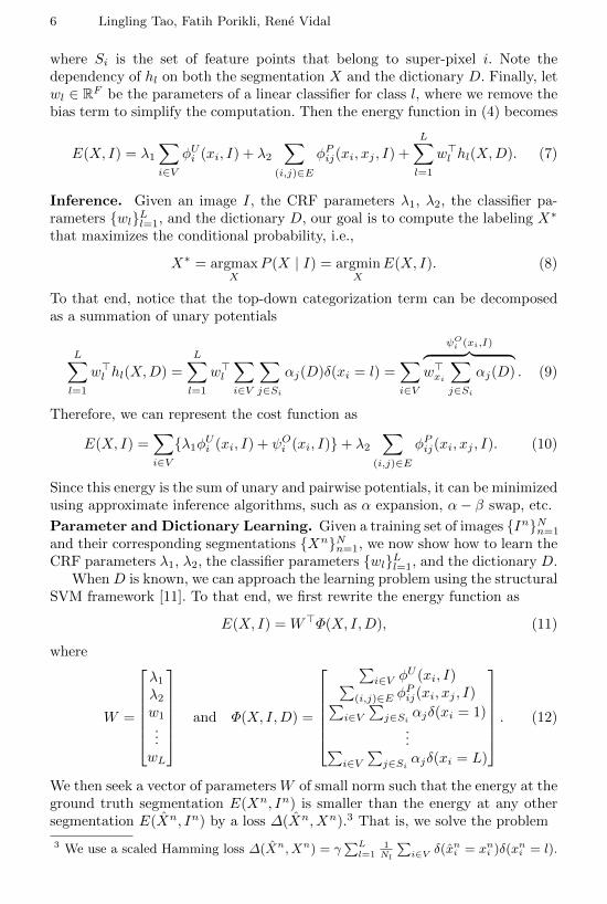
where Si is the set of feature points that belong to super-pixel i. Note thedependency of hl on both the segmentation X and the dictionary D. Finally, letwl ∈ RF be the parameters of a linear classifier for class l, where we remove thebias term to simplify the computation. Then the energy function in (4) becomes

E(X, I) = λ1∑i∈V


(i,j)∈E

φPij(xi, xj , I) +

L∑l=1

w>l hl(X,D). (7)

Inference. Given an image I, the CRF parameters λ1, λ2, the classifier pa-rameters {wl}Ll=1, and the dictionary D, our goal is to compute the labeling X∗

that maximizes the conditional probability, i.e.,

X∗ = argmaxX

P (X | I) = argminX

E(X, I). (8)

To that end, notice that the top-down categorization term can be decomposedas a summation of unary potentials

L∑l=1

w>l hl(X,D) =

L∑l=1

w>l∑i∈V

∑j∈Si

αj(D)δ(xi = l) =∑i∈V

ψOi (xi,I)︷︸︸︷

w>xi

∑j∈Si

αj(D) . (9)

Therefore, we can represent the cost function as

E(X, I) =∑i∈V{λ1φUi (xi, I) + ψOi (xi, I)}+ λ2

∑(i,j)∈E

φPij(xi, xj , I). (10)

Since this energy is the sum of unary and pairwise potentials, it can be minimizedusing approximate inference algorithms, such as α expansion, α− β swap, etc.

Parameter and Dictionary Learning. Given a training set of images {In}Nn=1

and their corresponding segmentations {Xn}Nn=1, we now show how to learn theCRF parameters λ1, λ2, the classifier parameters {wl}Ll=1, and the dictionary D.

When D is known, we can approach the learning problem using the structuralSVM framework [11]. To that end, we first rewrite the energy function as

E(X, I) = W>Φ(X, I,D), (11)

where

W =

λ1λ2w1

...wL

and Φ(X, I,D) =

∑i∈V φ

U (xi, I)∑(i,j)∈E φ

Pij(xi, xj , I)∑

i∈V∑j∈Si

αjδ(xi = 1)...∑

i∈V∑j∈Si

αjδ(xi = L)

. (12)

We then seek a vector of parameters W of small norm such that the energy at theground truth segmentation E(Xn, In) is smaller than the energy at any othersegmentation E(Xn, In) by a loss ∆(Xn, Xn).3 That is, we solve the problem

3 We use a scaled Hamming loss ∆(Xn, Xn) = γ∑L

l=11Nl

∑i∈V δ(x

ni = xni )δ(xni = l).


minW,{ξn}

1

2‖W‖2 +

C

N

N∑n=1

ξn

s.t. ∀n ∈ {1, . . . , N},∀Xn

W>Φ(Xn, In, D)−W>Φ(Xn, In, D) ≥ ∆(Xn, Xn)− ξn,

(13)

where {ξn} are slack variables that account for the violation of the constraints.The problem in (13) is a quadratic optimization problem subject to a combi-

natorial number of linear constraints in W , one for each labeling Xn. As shownin [11], this problem can be solved using a cutting plane method that alternatesbetween two steps: given W one finds the most violated constraint by solvingfor Xn = argminX{W>Φ(X, In, D)−∆(X,Xn)}, and given a set of constraintsXn one solves for W with this constraint added.

Unfortunately, in our case both W and D are unknown. Moreover, the energyis not linear in D and its dependency on D is not explicit. As a result, thecutting plane method does not apply to our problem. Therefore, we propose analternative approach inspired by recent work on image classification [1, 2, 31].

Let us first rewrite the optimization problem in (13) over both W and D as:

J(W,D) = (14)

1

2‖W‖2 +

C

N

N∑n=1

[W>Φ(Xn, In, D)−min

Xn

{W>Φ(Xn, In, D)−∆(Xn, Xn)}].

The basic idea is to solve this problem by stochastic gradient descent and the keychallenge is the computation of the gradient with respect to D. Let us denote thevariables after the t-th iteration as Dt and Wt, and the most violated constraintas {Xn

t }. We can easily compute the derivative of J with respect to W as:

∂J

∂W

∣∣∣Wt,Dt

= Wt +C

N

N∑n=1

(Φ(Xn, In, Dt)− Φ(Xnt , I

n, Dt)). (15)

To compute the derivative of J with respect to D, notice that J depends implic-itly on D through the sparse codes {αj}. Thus, we can compute ∂J/∂D usingthe chain rule, which requires computing ∂J/∂α and ∂α/∂D.

Under certain assumptions, ∂α/∂D can be computed as shown in [1, 2, 31].Specifically, since 0 has to be a subgradient of the objective function in (5), thesparse representation α of feature descriptor f must satisfy

D>(Dα− f) = −λ sign(α). (16)

Now, suppose that the support of α (denoted as Λ) does not change when thereis a small perturbation of D and let A = (D>ΛDΛ)−1, where DΛ is a submatrixof D whose columns are indexed by Λ. After taking the derivative of (16) withrespect to D we get:

∂α(k)

∂D= (f −Dα)A[k] − (DA>)〈k〉α

> ∀k ∈ Λ, (17)


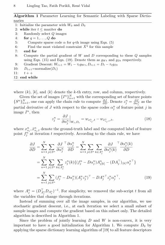
Algorithm 1 Parameter Learning for Semantic Labeling with Sparse Dictio-naries1: Initialize the parameter with W0 and D0

2: while iter t ≤ maxiter do3: Randomly select Q images4: for q = 1, . . . , Q do5: Compute sparse code α for q-th image using Eqn. (5)6: Find the most violated constraint Xq for this sample7: end for8: Compute the partial gradient of W and D corresponding to these Q samples

using Eqn. (15) and Eqn. (19). Denote them as gWt and gDt respectively.9: Gradient Descent: Wt+1 = Wt − τtgWt, Dt+1 = Dt − τtgDt

10: Dt+1=normalize(Dt)11: t+ +12: end while

where (k), [k], and 〈k〉 denote the k-th entry, row, and column, respectively.Given the set of images {In}Nn=1 with the corresponding set of feature points

{Sn}Nn=1, one can apply the chain rule to compute ∂J∂D . Denote znj = ∂J

∂αnj

as the

partial derivative of J with respect to the sparse codes αnj of feature point j inimage In, then

znj =∂J

∂αnj

∣∣∣Wt,Dt

= wxnsj,t − wxn

sj,t,t, (18)

where xnsj , xnsj ,t denote the ground-truth label and the computed label of feature

point fnj at iteration t respectively. According to the chain rule, we have

∂J

∂D=

N∑n=1

∑j∈Sn

∂J

∂αnj

> ∂αnj∂D

=

N∑n=1

∑j∈Sn

∑k∈Λn

j

∂J

∂αnj (k)

> ∂αnj (k)

∂D

=

N∑n=1

∑j∈Sn

∑k∈Λn

j

znj (k){(fnj −Dαnj )Anj[k] − (DA>j )〈k〉αnj>}

=

N∑n=1

∑j∈Sn

(fnj −Dαnj )(Anj znj )> −DAnj

>znj αnj>, (19)

where Anj = (D>ΛnjDΛn

j)−1. For simplicity, we removed the sub-script t from all

the variables that change through iterations.Instead of summing over all the image samples, in our algorithm, we use

stochastic gradient descent, i.e., at each iteration we select a small subset ofsample images and compute the gradient based on this subset only. The detailedalgorithm is described in Algorithm 1.

Since the problem of jointly learning D and W is non-convex, it is veryimportant to have a good initialization for Algorithm 1. We compute D0 byapplying the sparse dictionary learning algorithm of [19] to all feature descriptors


{fj}. We then compute W0 as [λ1, λ2, λ3w1, . . . , λ3wL], where {wl}Ll=1 are theparameters of a multi-class linear SVM classifier (without bias term) trained onthe histograms {hl(Xn, D0)}, and λ1, λ2, λ3 are the parameters of the model

E(X, I) = λ1∑i∈V

φU (xi, I) + λ2∑

(i,j)∈E

φPij(xi, xj , I) + λ3

L∑l=1

w>l hl(X,D0) (20)

trained on the segmentations {Xn} using standard structural SVM learning.

4 Experimental Results

Datasets. We evaluate our algorithm on three datasets: the Graz-02 dataset,the PASCAL VOC 2010 dataset and the MSRC21 dataset. The Graz-02 Dataset[23] contains 900 images of size 480×640. Each image is labeled with 4 categories:bike, pedestrian, car and background. In our experiments, we use 450 images fortraining and the other 450 for testing. The PASCAL VOC 2010 dataset [5]contains 1928 images labeled with 20 object classes and a background class.Following [14], since there is no publicly available groundtruth for the test data,we split the training/validation dataset and use 600 images among them fortraining, 364 for validation and 964 for testing. The MSRC21 dataset [25] consistsof 591 color images of size 320×213 and corresponding ground-truth labeling for21 classes. The standard train-validation-test split is used as described in [25].

Metric. We evaluate our algorithm using two performance metrics: accuracyand intersection-union metric (VOC measure). We compute the per-class accu-racy as the percentage of pixels that are classified correctly for each object class,and report the ’average’ accuracy (the mean of the per-class percentages) and the’global’ accuracy (the percentage of pixels from all classes that are classified cor-rectly). We compute the VOC measure for each object class as #TP

#TP+#FP+#FN ,where #TP , #FP and #FN are the number of true positives, false positives andfalse negatives, respectively, and report the mean VOC measure over all classes.

Top-down Term. Since this framework is general, it can be applied with dif-ferent unary, pairwise and top-down terms with different features. In our exper-iments, we used three different methods to extract feature points and computeobject-level histograms. In the first method (TP1), we extract sparse SIFT fea-tures for each image at detected interest points, similar to [26, 10]. In this case,each super-pixel region can contain 0, 1 or more feature points, and we use theabsolute value of the sparse code for our top-down term. In the second method(TP2), we extract one SIFT feature at the center of each super-pixel region, tocapture the texture of the whole region. In the third method (TP3), we computethe vectorized average TextonBoost scores of all pixels in each super-pixel asfeature points. In the last two methods, each super-pixel is associated with onlyone feature point. The first two methods are used for the Graz02 dataset, whilethe third method is used for both the PASCAL VOC and MSRC21 datasets.

Unary Potentials. We use different unary potentials for different datasets.For the Graz-02 dataset, we use the same unary potentials as in [26, 10] in order


to make our results comparable. Specifically, we first create super-pixels by over-segmenting each image using the Quick Shift algorithm [30]. Then we extractdense SIFT features on each image, and compute the BoF representation foreach super-pixel region. We then train an SVM with a χ2-RBF kernel usingLibSVM [4]. For each super-pixel, we apply the SVM classifier to the associatedhistogram and compute the logarithm of the output probability as the unarypotential. For the PASCAL VOC and MSRC21 datasets, we use the pixel-wiseunaries based on TextonBoost classifier provided by [14]. The super-pixel unarypotentials are then computed by first taking the logarithm of the probabilitiesand then averaging over all pixels inside each super-pixel.

Pairwise Potentials. For all datasets, we use a contrast sensitive costBij

1+‖Ci−Cj‖[10] as pairwise potentials, where Bij is the length of shared boundary betweensuper-pixel i and j, and Ci is the mean color of super-pixel i.

Implementation Details. We use the VL feat toolbox [29] for preprocessing.We use vl quickshift to generate super-pixels and set the parameter that controlssuper-pixel size to τ = 8. When extracting dense SIFT features to construct theunaries, we use the vl dsift function with spatial bin size set to 12. To definethe top-down cost, when computing sparse SIFT features (TP1), we apply thevl sift function with default settings, while for TP2, we set the position for SIFTfeatures to be the center position of each super-pixel, and the spatial bin size to8. For initializing the linear classifiers w1, . . . , wL, we use the Matlab StructuralSVM toolbox [28]. For initializing the dictionary and computing sparse represen-tations, we use the sparse coding toolbox provided by [19], where λ is set to 0.1,and the dictionary is of size 400 for SIFT feature points, and 50 for TextonBoostbased feature points. The parameter C in our Max-Margin formulation is set to1000. The scale γ of the hamming loss is set to 1000. For gradient descent, we usean initial step size τ0 =1e-6. We run 100 iterations for Graz02, and 600 iterationsfor PASCAL VOC and MSRC21. For PASCAL VOC and MSRC21, we use thevalidation data to train our parameters, while the unary potentials from [14] arecomputed based on training data. For Graz02, both unary potentials and modelparameters are computed based on training data.

4.1 Graz-02 Dataset

Results. Tables 1 and 2 show the VOC measure and per-class accuracy, re-spectively, on the Graz-02 dataset. Since we randomly sampled super-pixels tocompute the unary potentials for this dataset, we run the experiment 5 timesand calculate the mean and variance of the result (reported in parenthesis). Inthe tables, U+P refers to the basic CRF model described by Eqn. (2), and TP1and TP2 refer to the first two methods for extracting top-down feature points.Notice that the U+P result is computed by our implementation, while resultsfrom [26, 10] are taken from the original paper. To show that these results arecomparable, we observe that in [10], their U+P implementation gives an averageof 50.82% in VOC measure metric, and 80.36% in average per-class accuracy,which means our method and [10] are built based on comparable baselines.


Table 1. VOC measure on Graz-02Dataset

U+P [26] [10] Ours-TP1 Ours-TP2

BG 79.4 (0.8) 82.3 78.0 86.4 (0.1) 87.2 (0.1)

Bike 44.3 (0.3) 46.2 55.6 52.8 (0.1) 52.5 (0.1)

Car 40.6 (1.5) 36.5 41.5 44.1 (0.3) 48.4 (0.6)

Human 37.9 (1.2) 39.0 37.3 41.2 (0.8) 44.1 (0.6)

Mean 50.6 (0.3) 51.0 53.1 56.1 (0.1) 58.0 (0.1)

Table 2. Accuracy on Graz-02 Dataset

U+P [26] [10] Ours-TP1 Ours-TP2

BG 81.6 (0.3) 86.4 75.9 90.6 (0.1) 91.2 (0.1)

Bike 85.9 (0.1) 73.0 84.9 77.8 (1.7) 76.3 (0.5)

Car 78.9 (0.8) 68.7 76.7 66.3 (6.6) 68.2 (1.6)

Human 80.0 (1.4) 71.3 79.8 66.7 (5.5) 70.0 (1.2)

Mean 81.6 (0.1) 74.9 79.3 75.4 (0.6) 76.4 (0.1)

Global 81.72 (0.2) N/A N/A 87.6 (0.1) 88.1 (0.1)

Image Ground Truth U+P [26] Ours-TP1 Ours-TP2

Fig. 1. Example segmentation results for the Graz02 dataset using different methods.The background, bikes, cars and humans are color coded as blue, cyan, yellow and redrespectively.


Discussion. From Table 1 we can see that our method outperforms both ourbaseline U+P and other state-of-art methods (except for the bike category).However, the per-class accuracy in Table 2 is not improved except for the Back-ground category. This is understandable since our goal is to reduce the falsenegative rate as well as the false positive rate, while the accuracy metric focuseson the true positive rate exclusively. Note that for the Car and Human category,the VOC measure is improved by around 7% while the accuracy decreases byaround 10%. This implies that a lot of false positives are removed, i.e. less back-ground pixels are labeled as object. That is also why we observe improvementin both the accuracy and VOC measures for the Background class. Notice alsothat the performance for the Bike class decreases for our method. Our conjectureis that in the annotations of Graz02 the pixels inside the wheel are labeled asbike, while most of them are background except for the spokes. This leads todecreased performance, since some of the pixels inside the wheel are classified asbackground. We would expect better results with more detailed annotations.

We show some qualitative results in Fig. 1. As we can see, although moreforeground object pixels are labeled as background, the segmentation is moreaccurate at the boundaries and fewer superpixels from the background are la-beled as other class. For example, for the Bike category, our method can removefalse positives in the triangle area (row 2 in Fig. 1).

To further understand the effect of jointly learning the dictionary and theCRF parameters, we run experiments where only the weights W is updated,while the dictionary D is fixed. In this case, we achieve an average VOC measureof 50.1% for TP1 and 51.0% for TP2, which seems to suggest that for this dataset,updating the dictionary leads to majority of the improvement.

4.2 PASCAL VOC2010

Results. Fig. 2 shows the per-class VOC measure obtained by the baselinemethod (U+P) and our proposed method on the PASCAL VOC2010 datasetusing the third feature extraction method (TP3) to construct the top-down cat-egorization cost. In addition, Table 3 shows the average VOC measure obtainedby both methods together with the results of [25, 14, 33] for comparison. Thegrid-CRF method refers to the one used by [25], while its performance is re-ported in [14]. Notice that the dense-CRF in [14] models each pixel as a node ofthe graph, and the work in [33] uses also detection scores. On the other hand,our method adopts a super-pixel based CRF instead of a dense pixel based CRFand does not use any detection information directly. Therefore, it is more fair tocompare our results with those of the grid-CRF method in [25].

Discussion. As expected, our U+P baseline performs as good as the grid-CRFmodel, since they have similar graph size. Our method with jointly updatingdictionary and CRF leads to a 1.4% improvement in VOC measure and theperformance is comparable with more complex methods [14, 33]. As we can seein Fig. 2, for most of the object classes, we obtain an improvement of up to 5%.


!

0!0.1!0.2!0.3!0.4!0.5!0.6!0.7!0.8!0.9! U+P!

Ours4TP3!

Fig. 2. VOC measure on VOC 2010 dataset using baseline U+P and our method

Table 3. Results on VOC2010 Dataset

grid-CRF [25] dense-CRF [14] [33] U+P Ours-TP3

VOC measure 28.3 30.2 31.2 28.9 30.3

4.3 MSRC21

Results. Table 4 gives the mean and global accuracy obtained by the baselinemethod (U+P) and our proposed method on the MSRC21 dataset using theTextonBoost based unary potential and top-down terms, as for the PASCALVOC2010 dataset. The results of [24, 15, 14, 33] are also reported for comparison,while the performance of [15] on MSRC21 dataset is reported in [33]. We alsoshow some qualitative results in Fig. 3.

Discussion. The global accuracy given by our algorithm is slightly worse thanthat of other methods. However, the mean accuracy is on par with the perfor-mance of the dense-CRF model [14], and is only 1% less than the performance of[33]. As explained before, [33] combines both scene information and object infor-mation, while our method only uses TextonBoost feature. This suggests that ouralgorithm gives comparable result while using simpler models. Finally, while ourresults are just marginally better than those of the U+P baseline, when lookingat the example segmentations in in Fig. 3 we observe that our methods givesqualitatively better segmentations.


Table 4. Results on MSRC21 Dataset

Shotton HCRF Dense Yao U+P Ours-TP3et al. [24] + Coocc. [15] CRF [14] et al.[33]

Mean Accuracy 67 77.8 78.3 79.3 77.7 78.4

Global Accuracy 72 86.5 86.0 86.2 84.3 84.5

Image Ground Truth U+P Ours-TP3

Fig. 3. Example segmentation results for the MSRC21 dataset using the U+P baselineand our proposed method.

5 Conclusion

In this paper, we presented a new semantic segmentation framework that incor-porates a top-down object categorization cost based on a discriminative sparserepresentation of each object. We proposed an optimization framework to jointlylearn the sparse dictionary and the CRF parameters, so that the dictionary isspecifically trained for the segmentation task. Experimental results showed thatour algorithm outperforms the basic CRF model and the top-down model withBoF representation, suggesting that a jointly learned dictionary can help to im-prove segmentation performance compared with a pre-learned BoF dictionary.

Acknowledgements. We thank Florent Couzinie-Devy for interesting discus-sions about the gradient computation. The first and last author were supportedin part by grants NSF 1218709, ONR N000141310116 and ERC VideoWorld.Part of the work was conducted when the first two authors were at MitsubishiElectric Research Laboratories (MERL). This part was funded by MERL only.


References

1. Bach, F., Mairal, J., Ponce, J.: Task-driven dictionary learning. IEEE Transactionson Pattern Analysis and Machine Intelligence 34(4), 791–804 (2012)

2. Boureau, Y.L., Bach, F., LeCun, Y., Ponce, J.: Learning mid-level features forrecognition. In: IEEE Conference on Computer Vision and Pattern Recognition(2010)

3. Brostow, G.J., Shotton, J., Fauqueur, J., Cipolla, R.: Segmentation and recognitionusing structure from motion point clouds. In: European Conference on ComputerVision (2008)

4. Chang, C.C., Lin, C.J.: LIBSVM : a library for support vector machines (2001),software available at http://www.csie.ntu.edu.tw/ cjlin/libsvm

5. Everingham, M., Van Gool, L., Williams, C.K.I., Winn, J., Zisserman, A.: Thepascal visual object classes (voc) challenge. Int. Journal of Computer Vision 88(2),303–338 (2010)

6. Fei-Fei, L., Perona, P.: A bayesian hierarchical model for learning natural scenecategories. In: Computer Vision and Pattern Recognition, 2005. CVPR 2005. IEEEComputer Society Conference on (2005)

7. Fulkerson, B., Vedaldi, A., Soatto, S.: Class segmentation and object localiza-tion with superpixel neighborhoods. In: IEEE Int. Conference on Computer Vision(2009)

8. Galleguillos, C., Rabinovich, A., Belongie, S.: Object categorization using co-occurrence, location and appearance. In: IEEE Conference on Computer Visionand Pattern Recognition (2008)

9. Gould, S., Rodgers, J., Cohen, D., Elidan, G., Koller, D.: Multi-class segmentationwith relative location prior. International Journal of Computer Vision 80(3), 300–316 (2008)

10. Jain, A., Zappella, L., McClure, P., Vidal, R.: Visual dictionary learning for jointobject categorization and segmentation. In: European Conference on ComputerVision (2012)

11. Joachims, T., Finley, T., Yu, C.N.J.: Cutting-plane training of structural SVMs.Machine Learning 77(1), 27–59 (2009)

12. Kohli, P., Ladicky, L., Torr, P.H.S.: Robust higher order potentials for enforcing la-bel consistency. In: IEEE Conference on Computer Vision and Pattern Recognition(2008)

13. Kolmogorov, V., Zabih, R.: What energy functions can be minimized via graphcuts? IEEE Trans. on Pattern Analysis and Machine Intelligence 26(2), 147–159(2004)

14. Krahenbuhl, P., Koltun, V.: Efficient inference in fully connected crfs with gaussianedge potentials. In: Neural Information Processing Systems. pp. 109–117 (2011)

15. Ladicky, L., Sturgess, P., Alahari, K., Russell, C., Torr., P.: What, where andhow many? combining object detectors and CRFs. In: European Conference onComputer Vision (2010)

16. Ladicky, L., Russell, C., Kohli, P., Torr, P.: Associative hierarchical CRFs for objectclass image segmentation. In: IEEE Int. Conference on Computer Vision (2009)

17. Lafferty, J.D., McCallum, A., Pereira, F.C.N.: Conditional random fields: Proba-bilistic models for segmenting and labeling sequence data. In: ICML (2001)

18. Laptev, I.: On space-time interest points. International Journal of Computer Vision64(2-3), 107–123 (2005)


19. Lee, H., Battle, A., Raina, R., Ng, A.Y.: Efficient sparse coding algorithms. In:Neural Information Processing Systems. pp. 801–808 (2007)

20. Mairal, J., Bach, F., Ponce, J., Sapiro, G., Zisserman, A.: Discriminative learneddictionaries for local image analysis. IEEE Conference on Computer Vision andPattern Recognition (2008)

21. Murphy, K.P., Weiss, Y., Jordan, M.I.: Loopy belief propagation for approximateinference: An empirical study. In: Uncertainty in Artificial Intelligence. pp. 467–475(1999)

22. Naikal, N., Singaraju, D., Sastry, S.S.: Using models of objects with deformableparts for joint categorization and segmentation of objects. In: Asian Conference onComputer Vision (2013)

23. Opelt, A., Pinz, A.: The TU Graz-02 database.http://www.emt.tugraz.at/ pinz/data/GRAZ02/ (2002)

24. Shotton, J., Johnson, M., Cipolla, R.: Semantic texton forests for image catego-rization and segmentation. In: IEEE Conference on Computer Vision and PatternRecognition (2008)

25. Shotton, J., Winn, J.M., Rother, C., Criminisi, A.: Textonboost for image un-derstanding: Multi-class object recognition and segmentation by jointly modelingtexture, layout, and context. Int. Journal of Computer Vision 81(1), 2–23 (2009)

26. Singaraju, D., Vidal, R.: Using global bag of features models in random fields forjoint categorization and segmentation of objects. In: IEEE Conference on Com-puter Vision and Pattern Recognition (2011)

27. Tighe, J., Lazebnik, S.: Finding things: Image parsing with regions and per-exemplar detectors. In: IEEE Conference on Computer Vision and Pattern Recog-nition (2013)

28. Vedaldi, A.: A MATLAB wrapper of SVMstruct.http://www.vlfeat.org/ vedaldi/code/svm-struct-matlab.html (2011)

29. Vedaldi, A., Fulkerson, B.: VLFeat: An open and portable library of computervision algorithms. http://www.vlfeat.org/ (2008)

30. Vedaldi, A., Soatto, S.: Quick shift and kernel methods for mode seeking. In: Eu-ropean Conference on Computer Vision. pp. 705–718 (2008)

31. Yang, J., Yang, M.: Top-down visual saliency via joint CRF and dictionary learn-ing. In: IEEE Conference on Computer Vision and Pattern Recognition (2012)

32. Yang, J., Yu, K., Gong, Y., Huang, T.: Linear spatial pyramid matching usingsparse coding for image classification. In: IEEE Conference on Computer Visionand Pattern Recognition (2009)

33. Yao, J., Fidler, S., Urtasun, R.: Describing the scene as a whole: Joint objectdetection, scene classification and semantic segmentation. In: IEEE Conference onComputer Vision and Pattern Recognition (2012)

34. Yu, C.N.J., Joachims, T.: Learning structural SVMs with latent variables. In:Proceedings of the International Conference on Machine Learning. pp. 1169–1176(2009)

35. Zhang, K., Zhang, W., Zheng, Y., Xue, X.: Sparse reconstruction for weakly su-pervised semantic segmentation. In: International Joint Conference on ArtificialIntelligence. pp. 1889–1895 (2013)

Date post:	15-Feb-2019
Category:	Documents
Upload:	lediep
View:	221 times
Download:	0 times

Sparse Dictionaries for Semantic Segmentation -...

Documents