HAL Id: hal-00687445 https://hal.archives-ouvertes.fr/hal-00687445 Submitted on 13 Apr 2012 HAL is a multi-disciplinary open access archive for the deposit and dissemination of sci- entific research documents, whether they are pub- lished or not. The documents may come from teaching and research institutions in France or abroad, or from public or private research centers. L’archive ouverte pluridisciplinaire HAL, est destinée au dépôt et à la diffusion de documents scientifiques de niveau recherche, publiés ou non, émanant des établissements d’enseignement et de recherche français ou étrangers, des laboratoires publics ou privés. Sparsity-based optimization of two lifting-based wavelet transforms for semi-regular mesh compression Aymen Kammoun, Frédéric Payan, Marc Antonini To cite this version: Aymen Kammoun, Frédéric Payan, Marc Antonini. Sparsity-based optimization of two lifting-based wavelet transforms for semi-regular mesh compression. Computers and Graphics, Elsevier, 2012, 36 (4), pp.272-282. 10.1016/j.cag.2012.02.004. hal-00687445
Transcript
HAL Id: hal-00687445https://hal.archives-ouvertes.fr/hal-00687445
Submitted on 13 Apr 2012
HAL is a multi-disciplinary open accessarchive for the deposit and dissemination of sci-entific research documents, whether they are pub-lished or not. The documents may come fromteaching and research institutions in France orabroad, or from public or private research centers.
L’archive ouverte pluridisciplinaire HAL, estdestinée au dépôt et à la diffusion de documentsscientifiques de niveau recherche, publiés ou non,émanant des établissements d’enseignement et derecherche français ou étrangers, des laboratoirespublics ou privés.
Sparsity-based optimization of two lifting-based wavelettransforms for semi-regular mesh compression
Aymen Kammoun, Frédéric Payan, Marc Antonini
To cite this version:Aymen Kammoun, Frédéric Payan, Marc Antonini. Sparsity-based optimization of two lifting-basedwavelet transforms for semi-regular mesh compression. Computers and Graphics, Elsevier, 2012, 36(4), pp.272-282. �10.1016/j.cag.2012.02.004�. �hal-00687445�
Sparsity-based optimization of two lifting-based wavelettransforms forsemi-regular mesh compression
Aymen Kammoun, Frederic Payan and Marc Antonini
Laboratoire I3S, UMR CNRS - Universite de Nice Sophia Antipolis, France
Abstract
This paper describes how to optimize two popular wavelet transforms for semi-regular meshes, using lifting scheme.The objective is to adapt multiresolution analysis to the input mesh to improve its subsequent coding. Consider-ing either the Butterfly- or the Loop-based lifting schemes,our algorithm finds at each resolution level an optimalprediction operatorP such that it minimizes theL1-norm of the wavelet coefficients. The update operatorU is then re-computed in order to take into account the modifications toP. Experimental results show that our algorithm improveson state-of-the-art wavelet coders.
Wavelets have their roots in approximation theory [1]and signal processing [2] in the late eighties. Sincethen, wavelets are the most popular technique for rep-resenting data in a multiresolution way. They have beenused for a vast number of applications: physic, biomed-ical signal analysis, image processing, and so on. Butwavelets have been particularly designed for data cod-ing, because they guarantees compact representation oftransformed data, and consequently high compressionperformances.
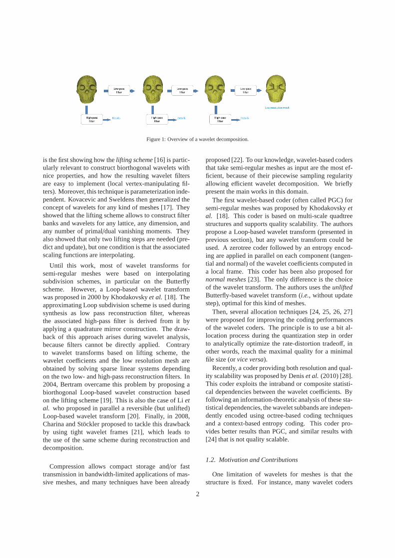
In computer graphics, the compact representation isnot the sole attractive feature of wavelets. Indeed,current high-resolution acquisition techniques producehighly detailed and densely sampled surface meshes.Not only these massive monoresolution data are diffi-cult to handle and store, but they are also awkward forfast and progressive transmission in bandwidth-limitedapplications. Wavelets tackle such issues, the multires-olution structure (Figure 1) making the progressive pro-cessing easier.
A problem for applying wavelets on meshes is the ir-regular sampling (unlike still images or videos). Despitethe development of wavelets for irregular meshes [3, 4],a popular solution is to remesh the input mesh semi-regularly (for instance with [5, 6, 7]) before applying
Email address:{kammoun,fpayan,am}@i3s.unice.fr(Aymen Kammoun, Frederic Payan and Marc Antonini)
wavelets. The principle is to resample the surface ge-ometry while providing a subdivision connectivity. Theoutput is called a semi-regular mesh, and wavelet filter-ing is finally more efficient.
1.1. Related work
Lounsberyet al. are considered as pioneers in thedevelopment of wavelets for surface meshes of arbi-trary topological type [8]. They proposed a techniqueto construct wavelets from any local, stationary, contin-uous, uniformly convergent subdivision schemes suchas Catmull-Clark [9], Loop [10], or Butterfly [11]. Thesubdivision scheme represents the synthesis filter, andthe analysis filter is derived from it. Two filters arefinally applied on the input mesh during analysis pro-viding respectively a mesh of low resolution (low-passfiltering), and a set of wavelet coefficients (high-pass fil-tering).
Inspired by the work of Lounsberyet al., and bythe work of Donoho concerning interpolating wavelettransforms [12], Schroder and Sweldens presented howbuilding wavelets for scalar functions specifically de-fined on a sphere [13]. They are not the first construct-ing wavelets on the sphere. The pioneers are Dahlkeetal. [14], who used a tensor product basis where one fac-tor is an exponential spline. A continuous transform andits semi-discretization have been also proposed by Free-den and Windheuser [15]. Nevertheless, the work ofSchroder and Sweldens in [13] is remarkable because it
Preprint submitted to Computers& Graphics February 10, 2012
Figure 1: Overview of a wavelet decomposition.
is the first showing how thelifting scheme[16] is partic-ularly relevant to construct biorthogonal wavelets withnice properties, and how the resulting wavelet filtersare easy to implement (local vertex-manipulating fil-ters). Moreover, this technique is parameterization inde-pendent. Kovacevic and Sweldens then generalized theconcept of wavelets for any kind of meshes [17]. Theyshowed that the lifting scheme allows to construct filterbanks and wavelets for any lattice, any dimension, andany number of primal/dual vanishing moments. Theyalso showed that only two lifting steps are needed (pre-dict and update), but one condition is that the associatedscaling functions are interpolating.
Until this work, most of wavelet transforms forsemi-regular meshes were based on interpolatingsubdivision schemes, in particular on the Butterflyscheme. However, a Loop-based wavelet transformwas proposed in 2000 by Khodakovskyet al. [18]. Theapproximating Loop subdivision scheme is used duringsynthesis as low pass reconstruction filter, whereasthe associated high-pass filter is derived from it byapplying a quadrature mirror construction. The draw-back of this approach arises during wavelet analysis,because filters cannot be directly applied. Contraryto wavelet transforms based on lifting scheme, thewavelet coefficients and the low resolution mesh areobtained by solving sparse linear systems dependingon the two low- and high-pass reconstruction filters. In2004, Bertram overcame this problem by proposing abiorthogonal Loop-based wavelet construction basedon the lifting scheme [19]. This is also the case of Lietal. who proposed in parallel a reversible (but unlifted)Loop-based wavelet transform [20]. Finally, in 2008,Charina and Stockler proposed to tackle this drawbackby using tight wavelet frames [21], which leads tothe use of the same scheme during reconstruction anddecomposition.
Compression allows compact storage and/or fasttransmission in bandwidth-limited applications of mas-sive meshes, and many techniques have been already
proposed [22]. To our knowledge, wavelet-based codersthat take semi-regular meshes as input are the most ef-ficient, because of their piecewise sampling regularityallowing efficient wavelet decomposition. We brieflypresent the main works in this domain.
The first wavelet-based coder (often called PGC) forsemi-regular meshes was proposed by Khodakovskyetal. [18]. This coder is based on multi-scale quadtreestructures and supports quality scalability. The authorspropose a Loop-based wavelet transform (presented inprevious section), but any wavelet transform could beused. A zerotree coder followed by an entropy encod-ing are applied in parallel on each component (tangen-tial and normal) of the wavelet coefficients computed ina local frame. This coder has been also proposed fornormal meshes[23]. The only difference is the choiceof the wavelet transform. The authors uses theunliftedButterfly-based wavelet transform (i.e., without updatestep), optimal for this kind of meshes.
Then, several allocation techniques [24, 25, 26, 27]were proposed for improving the coding performancesof the wavelet coders. The principle is to use a bit al-location process during the quantization step in orderto analytically optimize the rate-distortion tradeoff, inother words, reach the maximal quality for a minimalfile size (orvice versa).
Recently, a coder providing both resolution and qual-ity scalability was proposed by Deniset al. (2010) [28].This coder exploits the intraband or composite statisti-cal dependencies between the wavelet coefficients. Byfollowing an information-theoretic analysis of these sta-tistical dependencies, the wavelet subbands are indepen-dently encoded using octree-based coding techniquesand a context-based entropy coding. This coder pro-vides better results than PGC, and similar results with[24] that is not quality scalable.
1.2. Motivation and Contributions
One limitation of wavelets for meshes is that thestructure is fixed. For instance, many wavelet coders
2
use the Butterfly-based scheme [13]. From a com-pression point-of-view, this wavelet is relevant forsmooth surfaces because of the interpolating effect ofthe Butterfly scheme used as predictor, which producessmall coefficients. But this scheme is less efficient forother kinds of surfaces, with high frequency variationsor salient features, for instance. Finally, a waveletchanging in function of the geometric features ofthe input mesh could be a relevant tool. When thetransforms are lifting-based, this can be finally achievedby adapting the predict and update steps [29] to theinput mesh.
Therefore we propose an algorithm for optimizingtwo popular lifting-based wavelet transforms for semi-regular meshes: the Butterfly-based scheme [13], andthe Loop-based one [19]. Our motivation is to improvethe performances of the state-of-the-art wavelet coders,by adapting the multiresolution analysis tool to the fea-tures of the input mesh. The basic idea is to find, fora given semi-regular mesh, the prediction operator thatmaximizes the sparsity of wavelet coefficients at eachlevel of resolution. Indeed, it is well known in informa-tion theory that maximizing the data sparsity improvesthe coding performances [30].
The idea of adapting the prediction step of theButterfly-based scheme has been already introduced in[31]. The main contributions of the current paper are:
• More technical details about the optimization algo-rithm for the Butterfly-based lifting scheme;
• A more robust method for computing the updateoperator for this scheme. The reason is that thetechnique proposed in [31] sometimes fails be-cause of a potential null divisor;
• An extension of the optimization algorithm to theLoop-based lifting scheme [19], by taking into ac-count the features of this scheme.
The rest of this paper is organized as follows. Section2 introduces notions about semi-regular meshes and lift-ing scheme for semi-regular meshes. Section 3 and 4present our contributions, respectively for the Butterfly-based and the Loop-based lifting schemes. Section 5shows some experimental results, and we finally con-clude in section 6.
2. Background and notations
2.1. Semi-regular meshesA semi-regular meshML is based on a mesh hierar-
chy Ml (l ∈ {0, 1, ..., L}) that represents a given surface
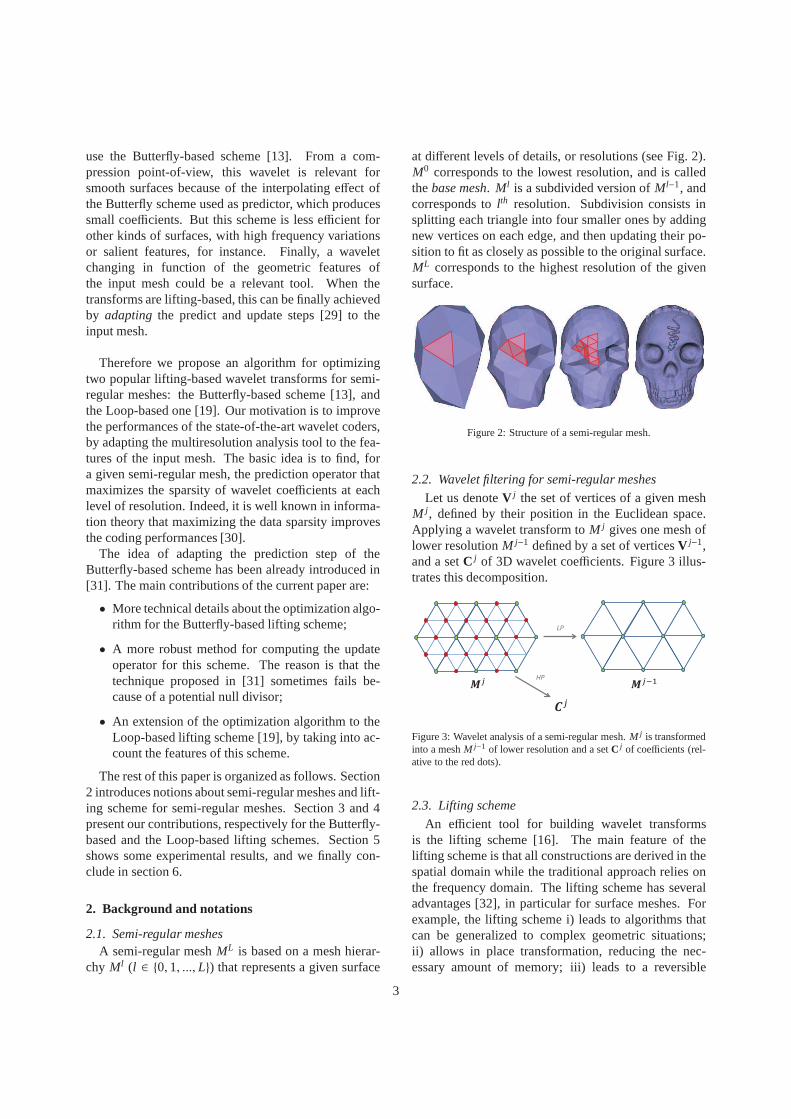
at different levels of details, or resolutions (see Fig. 2).M0 corresponds to the lowest resolution, and is calledthebase mesh. Ml is a subdivided version ofMl−1, andcorresponds tolth resolution. Subdivision consists insplitting each triangle into four smaller ones by addingnew vertices on each edge, and then updating their po-sition to fit as closely as possible to the original surface.ML corresponds to the highest resolution of the givensurface.
Figure 2: Structure of a semi-regular mesh.
2.2. Wavelet filtering for semi-regular meshes
Let us denoteV j the set of vertices of a given meshM j , defined by their position in the Euclidean space.Applying a wavelet transform toM j gives one mesh oflower resolutionM j−1 defined by a set of verticesV j−1,and a setC j of 3D wavelet coefficients. Figure 3 illus-trates this decomposition.
LP
HP
Figure 3: Wavelet analysis of a semi-regular mesh.M j is transformedinto a meshM j−1 of lower resolution and a setC j of coefficients (rel-ative to the red dots).
2.3. Lifting scheme
An efficient tool for building wavelet transformsis the lifting scheme [16]. The main feature of thelifting scheme is that all constructions are derived in thespatial domain while the traditional approach relies onthe frequency domain. The lifting scheme has severaladvantages [32], in particular for surface meshes. Forexample, the lifting scheme i) leads to algorithms thatcan be generalized to complex geometric situations;ii) allows in place transformation, reducing the nec-essary amount of memory; iii) leads to a reversible
3
implementation (analysis/synthesis), faster than im-plementation based on filter banks. Nevertheless, thelifting scheme has few drawbacks. For instance, the sta-bility of the transform is not guaranteed by construction.
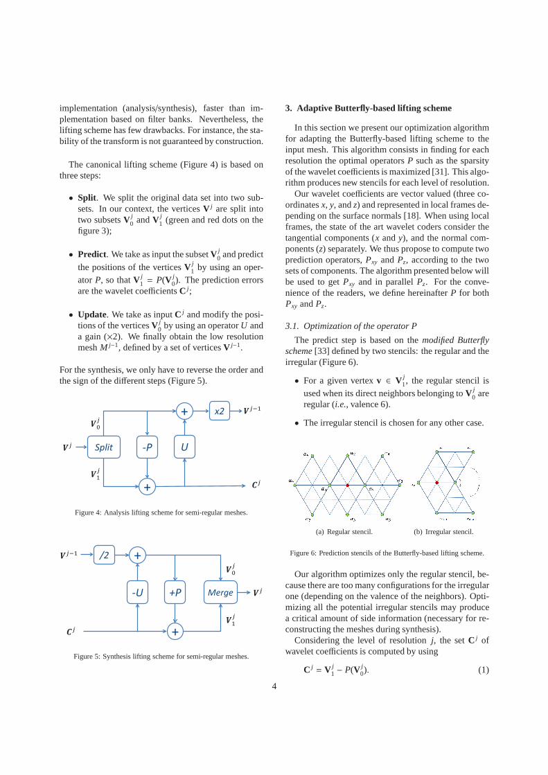
The canonical lifting scheme (Figure 4) is based onthree steps:
• Split. We split the original data set into two sub-sets. In our context, the verticesV j are split intotwo subsetsV j
0 andV j1 (green and red dots on the
figure 3);
• Predict. We take as input the subsetV j0 and predict
the positions of the verticesV j1 by using an oper-
ator P, so thatV j1 = P(V j
0). The prediction errorsare the wavelet coefficientsC j ;
• Update. We take as inputC j and modify the posi-tions of the verticesV j
0 by using an operatorU anda gain (×2). We finally obtain the low resolutionmeshM j−1, defined by a set of verticesV j−1.
For the synthesis, we only have to reverse the order andthe sign of the different steps (Figure 5).
+
Split -P U
+ x2
Figure 4: Analysis lifting scheme for semi-regular meshes.
/2
-U
+
+
+P Merge
Figure 5: Synthesis lifting scheme for semi-regular meshes.
3. Adaptive Butterfly-based lifting scheme
In this section we present our optimization algorithmfor adapting the Butterfly-based lifting scheme to theinput mesh. This algorithm consists in finding for eachresolution the optimal operatorsP such as the sparsityof the wavelet coefficients is maximized [31]. This algo-rithm produces new stencils for each level of resolution.
Our wavelet coefficients are vector valued (three co-ordinatesx, y, andz) and represented in local frames de-pending on the surface normals [18]. When using localframes, the state of the art wavelet coders consider thetangential components (x andy), and the normal com-ponents (z) separately. We thus propose to compute twoprediction operators,Pxy andPz, according to the twosets of components. The algorithm presented below willbe used to getPxy and in parallelPz. For the conve-nience of the readers, we define hereinafterP for bothPxy andPz.
3.1. Optimization of the operator P
The predict step is based on themodified Butterflyscheme[33] defined by two stencils: the regular and theirregular (Figure 6).
• For a given vertexv ∈ V j1, the regular stencil is
used when its direct neighbors belonging toV j0 are
regular (i.e., valence 6).
• The irregular stencil is chosen for any other case.
(a) Regular stencil. (b) Irregular stencil.
Figure 6: Prediction stencils of the Butterfly-based lifting scheme.
Our algorithm optimizes only the regular stencil, be-cause there are too many configurations for the irregularone (depending on the valence of the neighbors). Opti-mizing all the potential irregular stencils may producea critical amount of side information (necessary for re-constructing the meshes during synthesis).
Considering the level of resolutionj, the setC j ofwavelet coefficients is computed by using
C j = V j1 − P(V j
0). (1)
4
In order to increase the coding performances, wewantC j to become as sparse as possible. One solutionproposed in the literature is to minimize theL1-norm ofthis set [34]. So, maximizing the sparsity can be seen asthe minimization problem
minα j||V j
1 − Pα j (V j0)||1, (2)
whereα j defines the weights ofP for the level of reso-lution j.
To solve this problem, we define the unknown vec-
tor x =(
αj0, α
j1, . . . , α
j9
)Tcontaining the ten weights of
P, andN(v) the set of ten neighbor vertices ofV j0 and
depending on the regular stencil. We now define thematrix A of dimension (nr × 10)
A =[
N(V j1(0)) ; N(V j
1(1)) ; . . .N(V j1(nr − 1))
]
,(3)
wherenr is the number of vertices ofV j1 on which the
regular stencil is applied at this resolution. We then de-fine the vectorb
b =(
V j1(0),V j
1(1), . . .V j1(nr − 1)
)T. (4)
Finally, (2) can be solved by minimizing one functionf defined by
f : R10 7−→ Rx 7−→ f (x) = ||Ax − b||1. (5)
Since the Butterfly scheme is symmetric, we canwrite
α0 = α1
α2 = α3
α4 = α5 = α6 = α7
α8 = α9. (6)
Finally, the functionf has only four unknown values(α0, α2, α4 andα8) and can be written as following
f : R4 7−→ Rx 7−→ f (x) = ||Ax − b||1. (7)
This function f is convex (see Appendix A for de-tails) and bounded by 0, sof has a unique and globalminimum. To find this minimum, we use the Nelder-Mead simplex algorithm [35], but other algorithms maybe used. The proposed optimization algorithm is ap-plied to each level of resolution, successively from thehighest to the lowest.
3.2. Computation of the new operator U
Considering the same level of resolutionj and thecanonical lifting scheme (Figure 4), the set of verticesV j−1 is obtained by using
V j−1 = 2× (V j0 + U(C j)), (8)
whereU is the update operator depending on a weightγ and associated to the stencil given by Figure 7.
Figure 7: Update stencil of the Butterfly-based lifting scheme.
When the predictionP is based on a subdivision oper-ator, the updateU, that depends onP, has to be chosenfor obtaining vanishing moments [32].P being modi-fied at each level of resolution by the optimization al-gorithm, the weightγ of the update operatorU has tobe recomputed. In this work, we choose to computeγ such as to preserve the average betweenV j andV j−1.Contrary to [31], we prefer using the robust method pro-posed in [32]. The principle is to put all the vertices ofV j−1 and all the coefficients ofC j to zero, except onecoefficient ofC j put to 1 (see Figure 8).
Figure 8: Method for computingγ. The orange dot (a) represents theonly non null coefficient; the green dots (b) represent the two solevertices ofV j−1 with non null values after synthesis; the red dots rep-resent the 43 vertices ofV j with non null values after synthesis.
We apply the synthesis filters, and obtainV j . A ma-jority of the resulting vertices has null coordinates, ex-cept 43 over which the non null coefficient C j spread.These vertices are also shown on Figure 8. The valueassociated to each vertex are given by Table 1.
Table 1: Values of the 43 non null vertices ofV j obtaining after syn-thesis from only one non-null coefficient ofC j .
In this case, the average ofV j is equal to
143
(1− 2γ − 12γα0 − 12γα2 − 24γα4 − 12γα8) .(9)
Since the average ofV j−1 is null, equation (9) has to bealso null. We finally obtain
γ =1
2+ 12α0 + 12α2 + 24α4 + 12α8. (10)
3.3. Validation of the algorithm
To verify the efficiency of our optimization algorithm,we compare theL1-norm of the wavelet coefficientsobtained with the state of the art Butterfly-based lift-ing scheme (Classical), and with the proposed adaptivescheme (Optimized I). The results for Vase Lion are pre-sented in Table 2.
Table 2: L1-norm of the tangential and normal components (TCand NC) of the wavelet coefficients obtained with the state of theart Butterfly-based lifting scheme (Classical) and with our adaptivescheme (Optimized (I)) for Vase Lion. Optimized (II)is our adaptivescheme without constraint of symmetry.res is the level of resolution.
We observe that theL1-norm of each subset is glob-ally lower with our adaptive scheme. Similar results areobtained for all the experimented models, proving that
our algorithm works well. Nevertheless, for few mod-els (e.g. Vase Lion, Table 2), our algorithm does notdecrease theL1-norm of the tangential components oflowest resolution. This issue sometimes arises, only atthis resolution, when a majority of vertices are irregularand requires the irregular stencil. In this specific case,our optimization algorithm may not be effective at thisresolution but remains efficient for the other resolutions.
We also studied the influence of the constraint ofsymmetry (6) required by the prediction stencil. ThecolumnOptimized (II)presents the results of our algo-rithm without this constraint. We observe that the re-sults are similar. The constrained optimization processbeing three times faster (see Table 3), we finally retainthis variant for the experimentations (Section 5).
4. Adaptive Loop-based lifting scheme
As introduced in Section 1, we now expandour optimization technique to the Loop-based liftingscheme [19]. This transform, illustrated by figure 9, dif-fers from the canonical lifting scheme.
+
Split -P U2
+
-U1
+ /
Figure 9: Analysis Loop-based lifting scheme[19].
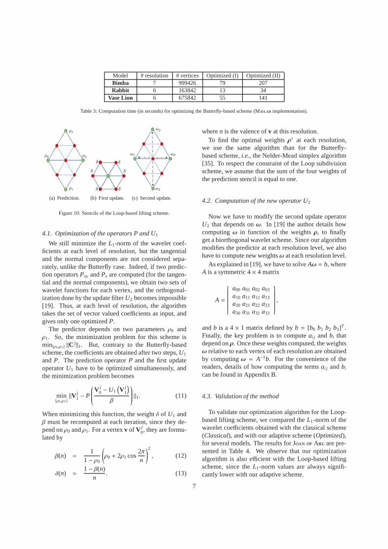
The main features of this scheme are:
• a prediction operatorP depending on two weightsρ0 andρ1 (see Figure 10(a));
• an update operatorU1 applied before the predictstep depending on a weightδ (see Figure 10(b)). Again 1
β(that depends on the valence of the vertices)
is also applied;
• a second operatorU2 depending on weightsω (seeFigure 10(c)). This step is applied to obtain abiorthogonal wavelet transform.
Note that the two update filters depend on the weightsρ
Table 3: Computation time (in seconds) for optimizing the Butterfly-based scheme (Matlab implementation).
(a) Prediction.
(b) First update.
(c) Second update.
Figure 10: Stencils of the Loop-based lifting scheme.
4.1. Optimization of the operators P and U1
We still minimize theL1-norm of the wavelet coef-ficients at each level of resolution, but the tangentialand the normal components are not considered sepa-rately, unlike the Butterfly case. Indeed, if two predic-tion operatorsPxy andPz are computed (for the tangen-tial and the normal components), we obtain two sets ofwavelet functions for each vertex, and the orthogonal-ization done by the update filterU2 becomes impossible[19]. Thus, at each level of resolution, the algorithmtakes the set of vector valued coefficients as input, andgives only one optimizedP.
The predictor depends on two parametersρ0 andρ1. So, the minimization problem for this scheme ismin{ρ0,ρ1} ||C
j ||1. But, contrary to the Butterfly-basedscheme, the coefficients are obtained after two steps,U1
andP. The prediction operatorP and the first updateoperatorU1 have to be optimized simultaneously, andthe minimization problem becomes
min{ρ0,ρ1}
||V j1 − P
V j0 − U1
(
V j1
)
β
||1. (11)
When minimizing this function, the weightδ of U1 andβ must be recomputed at each iteration, since they de-pend onρ0 andρ1. For a vertexv of V j
0, they are formu-lated by
β(n) =1
1− ρ0
(
ρ0 + 2ρ1 cos2πn
)2
, (12)
δ(n) =1− β(n)
n. (13)
wheren is the valence ofv at this resolution.To find the optimal weightsρ∗ at each resolution,
we use the same algorithm than for the Butterfly-based scheme,i.e., the Nelder-Mead simplex algorithm[35]. To respect the constraint of the Loop subdivisionscheme, we assume that the sum of the four weights ofthe prediction stencil is equal to one.
4.2. Computation of the new operator U2
Now we have to modify the second update operatorU2 that depends onω. In [19] the author details howcomputingω in function of the weightsρ, to finallyget a biorthogonal wavelet scheme. Since our algorithmmodifies the predictor at each resolution level, we alsohave to compute new weightsω at each resolution level.
As explained in [19], we have to solveAω = b, whereA is a symmetric 4× 4 matrix
A =
a00 a01 a02 a03
a10 a11 a12 a13
a20 a21 a22 a23
a30 a31 a32 a33
,
andb is a 4× 1 matrix defined byb = [b0 b1 b2 b3]T .Finally, the key problem is to computeai j andbi thatdepend onρ. Once these weights computed, the weightsω relative to each vertex of each resolution are obtainedby computingω = A−1b. For the convenience of thereaders, details of how computing the termsai j andbi
can be found in Appendix B.
4.3. Validation of the method
To validate our optimization algorithm for the Loop-based lifting scheme, we compared theL1-norm of thewavelet coefficients obtained with the classical scheme(Classical), and with our adaptive scheme (Optimized),for several models. The results for Joan of Arc are pre-sented in Table 4. We observe that our optimizationalgorithm is also efficient with the Loop-based liftingscheme, since theL1-norm values are always signifi-cantly lower with our adaptive scheme.
Table 4: L1-norm of the tangential and normal components (TC andNC) of the wavelet coefficients obtained with the state of the art Loop-based lifting scheme (Classical) and with our adaptive scheme (Opti-mized) for Joan of Arc. res is the level of resolution.
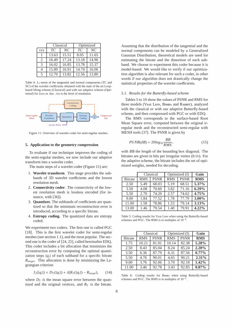
Wavelet Transform
Quantizer Entropy Coding
Connectivity Coding
Semi-regular
Mesh
ntropy
Specific Bitrate
Compressed
File +
Figure 11: Overview of wavelet coder for semi-regular meshes.
5. Application to the geometry compression
To evaluate if our technique improves the coding ofthe semi-regular meshes, we now include our adaptivetransform into a wavelet coder.
The main steps of a wavelet coder (Figure 11) are:
1. Wavelet transform. This stage provides the sub-bands of 3D wavelet coefficients and the lowestresolution mesh.
2. Connectivity coder. The connectivity of the low-est resolution mesh is lossless encoded (for in-stance, with [36]).
3. Quantizer. The subbands of coefficients are quan-tized so that the minimum reconstruction error isintroduced, according to a specific bitrate.
4. Entropy coding. The quantized data are entropycoded.
We experiment two coders. The first one is called PGC[18]. This is the first wavelet coder for semi-regularmeshes (see section 1.1), and the most popular. The sec-ond one is the coder of [24, 25], called hereinafter EDQ.This coder includes a bit allocation that minimizes thereconstruction error by computing the optimal quanti-zation steps{qi} of each subband for a specific bitrateRtarget. This allocation is done by minimizing the La-grangian criterion
Jλ({qi}) = DT({qi}) + λ(RT({qi}) − Rtarget), (14)
whereDT is the mean square error between the quan-tized and the original vertices, andRT is the bitrate.
Assuming that the distribution of the tangential and thenormal components can be modeled by a GeneralizedGaussian Distribution, theoretical models are used forestimating the bitrate and the distortion of each sub-band. We choose to experiment this coder because it ismodel-based. We would like to verify if our optimiza-tion algorithm is also relevant for such a coder, in otherwords if our algorithm does not drastically change thestatistical properties of the wavelet coefficients.
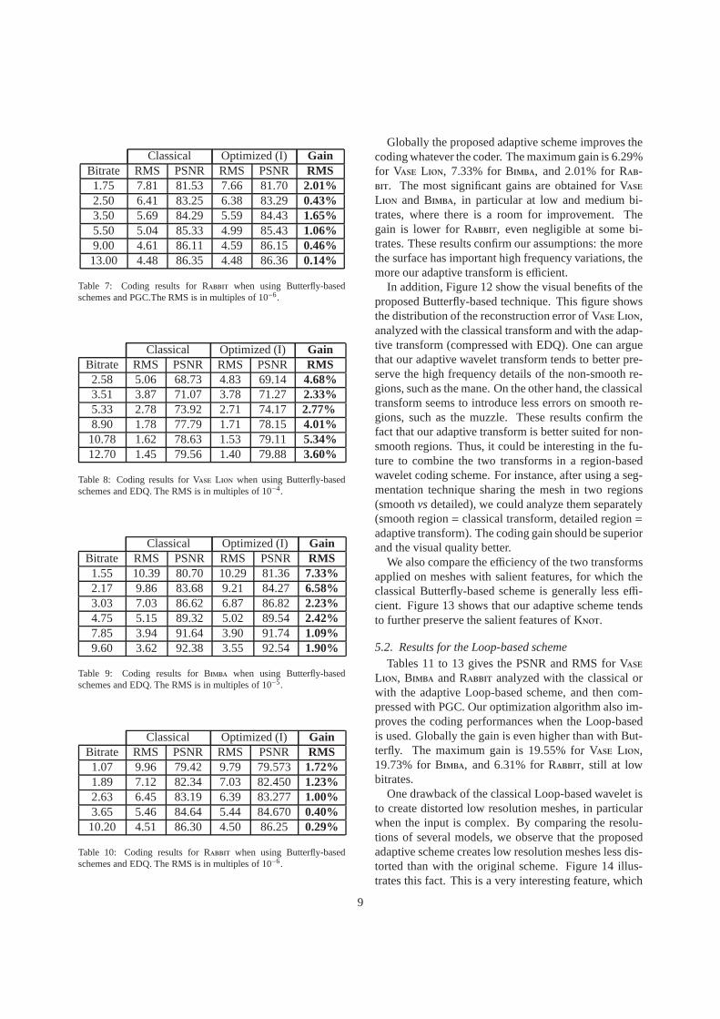
5.1. Results for the Butterfly-based scheme
Tables 5 to 10 show the values of PSNR and RMS forthree models (Vase Lion, Bimba and Rabbit), analyzedwith the classical or with our adaptive Butterfly-basedscheme, and then compressed with PGC or with EDQ.
The RMS corresponds to the surface-based RootMean Square error, computed between the original ir-regular mesh and the reconstructed semi-regular withMESH tools [37]. The PSNR is given by
PS NR(dB) = 20log10BB
RMS, (15)
with BB the length of the bounding box diagonal. Thebitrates are given in bits per irregular vertex (b/iv). Forthe adaptive scheme, the bitrate includes the set of opti-mized weights, needed for decoding.
Table 10: Coding results for Rabbit when using Butterfly-basedschemes and EDQ. The RMS is in multiples of 10−6.
Globally the proposed adaptive scheme improves thecoding whatever the coder. The maximum gain is 6.29%for Vase Lion, 7.33% for Bimba, and 2.01% for Rab-bit. The most significant gains are obtained for VaseLion and Bimba, in particular at low and medium bi-trates, where there is a room for improvement. Thegain is lower for Rabbit, even negligible at some bi-trates. These results confirm our assumptions: the morethe surface has important high frequency variations, themore our adaptive transform is efficient.
In addition, Figure 12 show the visual benefits of theproposed Butterfly-based technique. This figure showsthe distribution of the reconstruction error of Vase Lion,analyzed with the classical transform and with the adap-tive transform (compressed with EDQ). One can arguethat our adaptive wavelet transform tends to better pre-serve the high frequency details of the non-smooth re-gions, such as the mane. On the other hand, the classicaltransform seems to introduce less errors on smooth re-gions, such as the muzzle. These results confirm thefact that our adaptive transform is better suited for non-smooth regions. Thus, it could be interesting in the fu-ture to combine the two transforms in a region-basedwavelet coding scheme. For instance, after using a seg-mentation technique sharing the mesh in two regions(smoothvsdetailed), we could analyze them separately(smooth region= classical transform, detailed region=adaptive transform). The coding gain should be superiorand the visual quality better.
We also compare the efficiency of the two transformsapplied on meshes with salient features, for which theclassical Butterfly-based scheme is generally less effi-cient. Figure 13 shows that our adaptive scheme tendsto further preserve the salient features of Knot.
5.2. Results for the Loop-based schemeTables 11 to 13 gives the PSNR and RMS for Vase
Lion, Bimba and Rabbit analyzed with the classical orwith the adaptive Loop-based scheme, and then com-pressed with PGC. Our optimization algorithm also im-proves the coding performances when the Loop-basedis used. Globally the gain is even higher than with But-terfly. The maximum gain is 19.55% for Vase Lion,19.73% for Bimba, and 6.31% for Rabbit, still at lowbitrates.
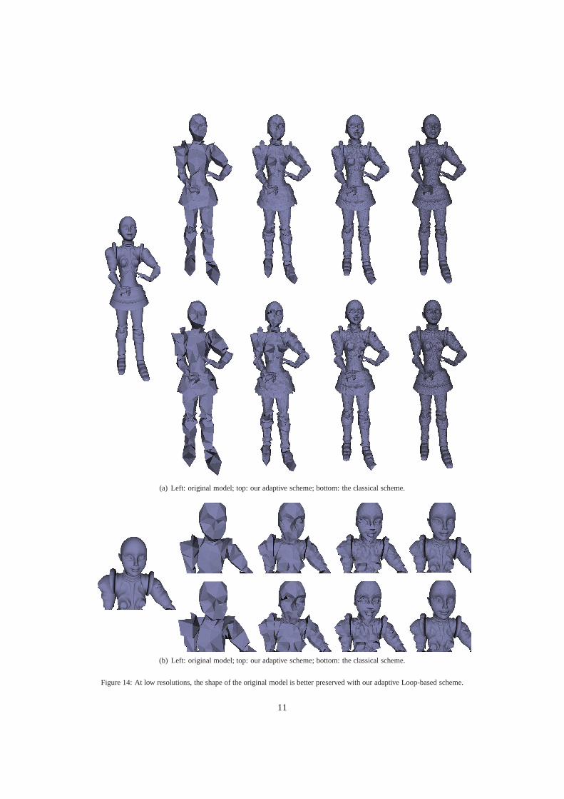
One drawback of the classical Loop-based wavelet isto create distorted low resolution meshes, in particularwhen the input is complex. By comparing the resolu-tions of several models, we observe that the proposedadaptive scheme creates low resolution meshes less dis-torted than with the original scheme. Figure 14 illus-trates this fact. This is a very interesting feature, which
9
(a) Classical wavelet. (b) Adaptive wavelet.
Figure 12: Distribution of the reconstruction error of Vase Lion, analyzed with the classical and with the adaptive Butterfly-based scheme (com-pressed with EDQ). The color corresponds to the magnitude ofthe distance point-surface computed between the original mesh and the compressed(MESH tools).
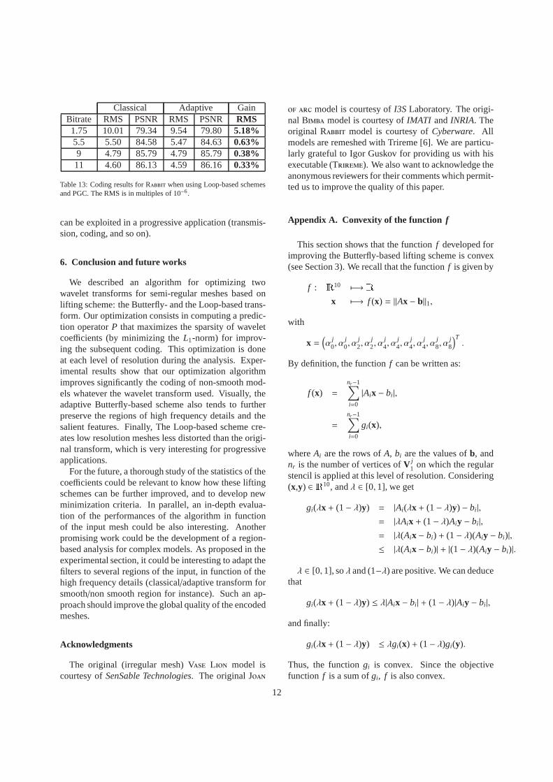
Table 13: Coding results for Rabbit when using Loop-based schemesand PGC. The RMS is in multiples of 10−6.
can be exploited in a progressive application (transmis-sion, coding, and so on).
6. Conclusion and future works
We described an algorithm for optimizing twowavelet transforms for semi-regular meshes based onlifting scheme: the Butterfly- and the Loop-based trans-form. Our optimization consists in computing a predic-tion operatorP that maximizes the sparsity of waveletcoefficients (by minimizing theL1-norm) for improv-ing the subsequent coding. This optimization is doneat each level of resolution during the analysis. Exper-imental results show that our optimization algorithmimproves significantly the coding of non-smooth mod-els whatever the wavelet transform used. Visually, theadaptive Butterfly-based scheme also tends to furtherpreserve the regions of high frequency details and thesalient features. Finally, The Loop-based scheme cre-ates low resolution meshes less distorted than the origi-nal transform, which is very interesting for progressiveapplications.
For the future, a thorough study of the statistics of thecoefficients could be relevant to know how these liftingschemes can be further improved, and to develop newminimization criteria. In parallel, an in-depth evalua-tion of the performances of the algorithm in functionof the input mesh could be also interesting. Anotherpromising work could be the development of a region-based analysis for complex models. As proposed in theexperimental section, it could be interesting to adapt thefilters to several regions of the input, in function of thehigh frequency details (classical/adaptive transform forsmooth/non smooth region for instance). Such an ap-proach should improve the global quality of the encodedmeshes.
Acknowledgments
The original (irregular mesh) Vase Lion model iscourtesy ofSenSable Technologies. The original Joan
of arc model is courtesy ofI3SLaboratory. The origi-nal Bimba model is courtesy ofIMATI andINRIA. Theoriginal Rabbit model is courtesy ofCyberware. Allmodels are remeshed with Trireme [6]. We are particu-larly grateful to Igor Guskov for providing us with hisexecutable (Trireme). We also want to acknowledge theanonymous reviewers for their comments which permit-ted us to improve the quality of this paper.
Appendix A. Convexity of the function f
This section shows that the functionf developed forimproving the Butterfly-based lifting scheme is convex(see Section 3). We recall that the functionf is given by
f : R10 7−→ Rx 7−→ f (x) = ||Ax − b||1,
with
x =(
αj0, α
j0, α
j2, α
j2, α
j4, α
j4, α
j4, α
j4, α
j8, α
j8
)T.
By definition, the functionf can be written as:
f (x) =
nr−1∑
i=0
|Aix − bi |,
=
nr−1∑
i=0
gi(x),
whereAi are the rows ofA, bi are the values ofb, andnr is the number of vertices ofV j
1 on which the regularstencil is applied at this level of resolution. Considering(x,y) ∈ R10, andλ ∈ [0, 1], we get
gi(λx + (1− λ)y) = |Ai(λx + (1− λ)y) − bi |,
= |λAix + (1− λ)Aiy − bi |,
= |λ(Aix − bi) + (1− λ)(Aiy − bi)|,
≤ |λ(Aix − bi)| + |(1− λ)(Aiy − bi)|.
λ ∈ [0, 1], soλ and (1−λ) are positive. We can deducethat
gi(λx + (1− λ)y) ≤ λ|Aix − bi | + (1− λ)|Aiy − bi |,
and finally:
gi(λx + (1− λ)y) ≤ λgi(x) + (1− λ)gi(y).
Thus, the functiongi is convex. Since the objectivefunction f is a sum ofgi, f is also convex.
12
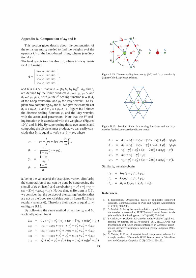
Appendix B. Computation of ai j and bi
This section gives details about the computation ofthe termsai j andbi needed to find the weightsρ of theoperatorU2 of the Loop-based lifting scheme (see Sec-tion 4.2).The final goal is to solveAω = b, whereA is a symmet-ric 4× 4 matrix
A =
a00 a01 a02 a03
a10 a11 a12 a13
a20 a21 a22 a23
a30 a31 a32 a33
,
andb is a 4× 1 matrix b = [b0 b1 b2 b3]T . ai j andbi
are defined by the inner productsai j =< φi , φ j > andbi =< ψl , φi >, with φi the ith scaling function (i = 0..4)of the Loop transform, andψl the lazy wavelet. To ex-plain how computingai j andbi , we give the examples ofb1 =< ψl , φ1 > anda11 =< φ1, φ1 >. Figure B.15 showsthe discrete scaling functionφ1 and the lazy wavelet,with the associated parameters. Note that theith scal-ing functionφi is associated with the weightωi (Figures10(c) and B.16). By superposing those two stencils andcomputing the discrete inner product, we can easily con-clude thatb1 is equal toγ0δ0 + α1δ1 + ρ0, where
αi = ρ0 +
(
ρ0 + 2ρ1 cos2πni
)2
,
βi =1
1− ρ0(αi − ρ0) ,
γi =1− αi
ni,
δi =1− βi
ni,
ni being the valence of the associated vertex. Similarly,the computation ofa11 can be done by superposing thestencil ofφ1 on itself, and we obtainγ2
0 +α21+ γ
22 + γ
23 +
(n1−3)γ26+n1(ρ2
0+ ρ21). Notice that, as Bertram in [19],
we consider that the vertices of the scaling functions thatare not on the Loop stencil (blue dots on figure B.16) areregular (valence 6). Therefore their value is equal toγ6
on Figure B.15.By following the same method on all theai j andbi ,
we finally obtain forA
a00 = α20 + γ
21 + γ
22 + γ
23 + (n0 − 3)γ2
6 + n0(ρ20 + ρ
21)
a01 = a10 = α0γ0 + γ1α1 + γ22 + γ
23 + ρ
20 + 4ρ0ρ1
a02 = a20 = α0γ0 + γ21 + γ2α2 + γ
26 + ρ
20 + 4ρ0ρ1
a03 = a30 = α0γ0 + γ21 + γ
26 + γ3α3 + ρ
20 + 4ρ0ρ1
a11 = γ20 + α
21 + γ
22 + γ
23 + (n1 − 3)γ2
6 + n1(ρ20 + ρ
21)
1
Figure B.15: Discrete scaling functionφ1 (left) and Lazy waveletψl
(right) of the Loop-based scheme.
Figure B.16: Position of the four scaling functions and the lazywavelet for the Loop-based prediction stencil.
a12 = a21 = γ20 + α1γ1 + γ2α2 + γ
26 + ρ
20 + 4ρ0ρ1
a13 = a31 = γ20 + α1γ1 + γ
26 + γ3α3 + ρ
20 + 4ρ0ρ1
a22 = γ20 + γ
21 + α
22 + (n2 − 2)γ2
6 + n2(ρ20 + ρ
21)
a23 = a32 = γ20 + γ
21 + ρ
21
a33 = γ20 + γ
21 + α
23 + (n3 − 2)γ2
6 + n3(ρ20 + ρ
21).
Similarly, we also obtain
b0 = (α0δ0 + γ1δ1 + ρ0)
b1 = (γ0δ0 + α1δ1 + ρ0)
b2 = b3 = (γ0δ0 + γ1δ1 + ρ1).
References
[1] I. Daubechies, Orthonormal bases of compactly supportedwavelets, Communications on Pure and Applied Mathematics41 (1988) 909–996.
[2] S. Mallat, A theory for multiresolution signal decomposition:the wavelet representation, IEEE Transactions on Pattern Anal-ysis and Machine Intelligence 11 (7) (1989) 674–693.
[3] I. Guskov, W. Sweldens, P. Schroder, Multiresolution signal pro-cessing for meshes, in: A. Rockwood (Ed.), SIGGRAPH ’99:Proceedings of the 26th annual conference on Computer graph-ics and interactive techniques, Addison Wesley Longman, 1999,pp. 325–334.
[4] S. Valette, R. Prost, A wavelet based compression schemefortriangle meshes : Wavemesh, IEEE Transactions on Visualiza-tion and Computer Graphics 10 (2) (2004) 123–133.
13
[5] I. Friedel, P. Schroder, A. Khodakovsky, Variational normalmeshes, ACM Transactions on Graphics 23 (4) (2004) 1061–1073. doi:http://doi.acm.org/10.1145/1027411.1027418.
[6] I. Guskov, Manifold-based approach to semi-regularremeshing, Graphical Models 69 (1) (2007) 1–18.doi:http://dx.doi.org/10.1016/j.gmod.2006.05.001.
[7] A. Kammoun, F. Payan, M. Antonini, Adaptive semi-regularremeshing: A voronoi-based approach, in: Proceedings of IEEEinternational workshop on MultiMedia Signal Processing, Saint-Malo, France, 2010, pp. 350–355.
[8] M. Lounsbery, T. D. DeRose, J. Warren, Multiresolution analy-sis for surfaces of arbitrary topological type, ACM Transactionson Graphics 16 (1) (1997) 34–73.
[9] E. Catmull, J. Clark, Recursively generated B-spline surfaces onarbitrary topological meshes, Computer-aided Design 10 (1978)350–355. doi:10.1016/0010-4485(78)90110-0.
[10] C. Loop, Smooth subdivision surfaces based on triangles, Mas-ter’s thesis, University of Utah (1987).
[11] N. Dyn, D. Levin, J. Gregory, A butterfly subdivision scheme forsurface interpolation with tension control, ACM Transactions onGraphics 9 (2) (1990) 160–169.
[12] D. L. Donoho, Interpolating wavelet transforms, Preprint, De-partment of Statistics, Stanford University (1992).
[13] P. Schroder, W. Sweldens, Spherical wavelets: efficiently rep-resenting functions on the sphere, in: Proceedings of the 22ndannual conference on Computer graphics and interactive tech-niques, SIGGRAPH ’95, ACM, New York, NY, USA, 1995, pp.161–172.
[14] S. Dahlke, W. Dahmen, I. Weinreich, E. Schmitt, Multiresolu-tion analysis and wavelets on s2 and s3, Numerical functionalanalysis and optimization 16 (1,2) (1995) 19–41.
[15] W. Freeden, U. Windheuser, Spherical wavelet transform and itsdiscretization, Advances in Computational Mathematics 5 (1)(1996) 51–94.
[16] W. Sweldens, The lifting scheme: A construction of secondgeneration wavelets, SIAM Journal on Mathematical Analysis29 (2) (1998) 511–546.
[17] J. Kovacevic, W. Sweldens, Wavelet families of increasing orderin arbitrary dimensions, IEEE Transactions on Image Processing9 (3) (2000) 480–496.
[18] A. Khodakovsky, P. Schroder, W. Sweldens, Progressive geom-etry compression, in: SIGGRAPH’00 Proceedings of the 27thannual conference on Computer graphics and interactive tech-niques, ACM Press/Addison-Wesley Publishing Co., 2000, pp.271–278.
[20] D. Li, K. Qin, H. Sun, Unlifted loop subdivision wavelets,Pacific Conference on Computer Graphics and Applications 0(2004) 25–33.
[21] M. Charina, J. Stockler, Tight wavelet frames for subdivision,Journal of Computational and Applied Mathematics 221 (2)(2008) 293–301.
[22] P. Jingliang, K. Chang-Su, C.-C. J. Kuo, Technologies for 3Dmesh compression: A survey, Journal of Visual Communicationand Image Representation 16 (2005) 688–733.
[23] A. Khodakovsky, I. Guskov, Compression of normal meshes,in: Geometric Modeling for Scientific Visualization, Springer-Verlag, 2003, pp. 189–206.
[24] F. Payan, M. Antonini, An efficient bit allocation for compress-ing normal meshes with an error-driven quantization, ElsevierComputer Aided Geometry Design 22 (5) (2005) 466–486.
[25] F. Payan, M. Antonini, Mean square error approximationforwavelet-based semiregular mesh compression, IEEE Transac-tions on Visualization and Computer Graphics (TVCG) 12 (5)
(2006) 649–657.[26] J.-Y. Sim, C.-S. Kim, C. J. Kuo, S.-U. Lee, Normal mesh com-
pression based on rate-distortion optimization, in: Proceedingsof the IEEE Workshop on MultiMedia Signal Processing, 2002,pp. 13–16.
[27] S. Lavu, H. Choi, R. Baraniuk, Geometry compression of nor-mal meshes using rate-distortion algorithms, in: Proceedings ofthe Eurographics/ACM SIGGRAPH symposium on Geometryprocessing, Vol. 43, 2003, pp. 52–61.
[28] L. Denis, S. M. Satti, A. Munteanu, J. Cornelis, P. Schelkens,Scalable intraband and composite wavelet-based coding ofsemiregular meshes, IEEE Transactions on Multimedia 12 (8)(2010) 773–789.
[29] G. Piella, H. J. A. M. Heijmans, H. J. A. M. Heijmans, Adaptivelifting schemes with perfect reconstruction, IEEE Transactionson Signal Processing 50 (2001) 1620–1630.
[30] S. Mallat, A wavelet tour of signal processing, Academic Press,1998.
[31] A. Kammoun, F. Payan, M. Antonini, Optimized butterfly-basedlifting scheme for semi-regular meshes, in: Proceedings ofIEEEInternational Conference in Image Processing (ICIP), Brussels,Belgium, 2011, pp. 1293–1296.
[32] P. Schroder, W. Sweldens, M. Cohen, T. DeRose, D. Salesin,Wavelets in computer graphics, SIGGRAPH Course notes(1996).
[33] D. Zorin, P. Schroder, W. Sweldens, Interpolating subdivisionfor meshes with arbitrary topology, in: Proceedings of SIG-GRAPH 96, 1996, pp. 189–192.
[34] D. Donoho, Y. Tsaig, Fast solution of l1-norm minimizationproblems when the solution may be sparse, IEEE Transactionson Information Theory 54 (11) (2008) 4789–4812.
[35] J. C. Lagarias, J. C. Lagarias, J. A. Reeds, J. A. Reeds, M. H.Wright, M. H. Wright, P. E. Wright, P. E. Wright, Convergenceproperties of the nelder-mead simplex algorithm in low dimen-sions, SIAM Journal of Optimization 9 (1996) 112–147.
[36] C. Touma, C. Gotsman, Triangle mesh compression, GraphicsInterface’98 (1998) 26–34.
[37] N. Aspert, D. Santa-Cruz, T. Ebrahimi, Mesh: Measuringerrorsbetween surfaces using the hausdorff distance, in: IEEE Inter-national Conference in Multimedia and Expo (ICME), Vol. 1,2002, pp. 705–708.